Robust analyses for longitudinal clinical trials with missing and non-normal continuous outcomes

Study 193A conducted by the AIDS Clinical Trial Group compares the effects of dual or triple combinations of the HIV-1 reverse transcriptase inhibitors (Henry et al. 1998). The data consists of the longitudinal outcomes of the CD4 count data at baseline and during the first 40 weeks of follow-up, with the fully-observed baseline covariates as age and gender. In the trial, the participants are randomly assigned among the four treatments regarding dual or triple therapies. We focus on the treatment comparison between arm 1 (zidovudine alternating monthly with 400 mg didanosine) and arm 2 (zidovudine plus 400mg of didanosine plus 400mg of nevirapine). As arm 1 involves fewer combinations of inhibitors than arm 2, we view it as the reference group. Among individuals in these two arms, we delete the ones with missing baseline CD4 counts, partition the time into discrete intervals $(0,12]$, $(12,20]$, $(20,28]$, $(28,36]$ and $(36,40]$, and create a dataset with a monotone missingness pattern.

Since the original CD4 counts are highly skewed, we conduct a log transformation to get the transformed CD4 counts as $\log(\text{CD4}+1)$ and use them as the outcomes of interest. Figure 1 presents the spaghetti plots of the transformed CD4 counts. Although there are no outstanding outliers, severe missingness is evident in the data, with only 34 of 320 participants in arm 1 and 46 of 330 participants in arm 2 completing the trial. The high dropout rates in this data reflect a typical missing data issue in longitudinal clinical trials, leading to the demand of conducting imputation for the missing components to prevent the substantial information loss if we focus on only the complete data.

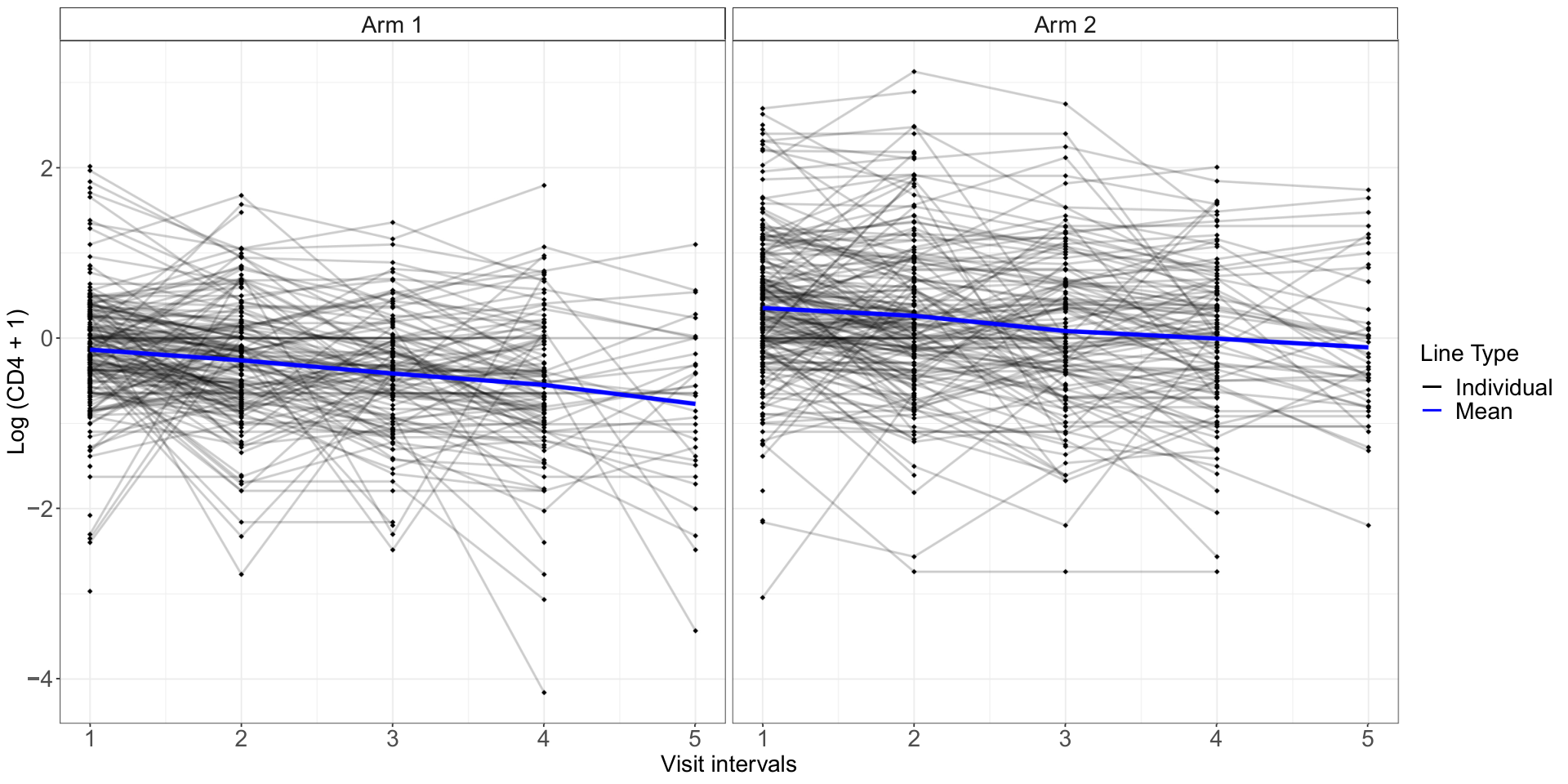
We check the normality of the data by fitting sequential linear regressions on the current outcomes against all historical information and examining the conditional residuals at each visit point for model diagnosis. An assessment of the normality of the responses via the Shapiro-Wilk test and the normal QQ plots are presented in Figure 2. Each normality test indicates a violation of the normal assumption, and the normal QQ plots reveal that the CD4 counts remain heavy-tailed even after the log transformation. Under this circumstance, potentially biased and inefficient treatment effect estimates may occur when applying the conventional MI along with the MMRM analysis. It motivates the development of a robust method to assess the treatment effect precisely under non-normality.

Consider a longitudinal clinical trial with $n$ participants and $t$ follow-up visits. Let $A_{i}$ be the binary treatment without loss of generality, $X_{i}$ be the $p$-dimensional fully-observed baseline covariates including the intercept term with a full-column rank, $Y_{is}$ be the continuous outcome of interest at visit $s$, where $i=1,\cdots,n$, and $s=1,\cdots,t$. In longitudinal clinical trials, participants are randomly assigned to different treatment groups with non-zero probabilities. When missingness is involved, denote the observed indicator at visit $s$ as $R_{is}$, where $R_{is}=1$ if $Y_{is}$ is observed and $R_{is}=0$ otherwise. We assume a monotone missingness pattern throughout the paper, i.e., if the missingness begins at visit $s$, we have $R_{is^{\prime}}=1$ for $s^{\prime}<s$ and $R_{is^{\prime}}=0$ for $s^{\prime}\geq s$. Denote $H_{is}=(X_{i}^{\text{T}},Y_{i1},\cdots,Y_{is})^{\text{T}}$ as the history up to visit $s$, with $H_{i0}=X_{i}$. Since the outliers in the baseline covariates can be identified and removed by data inspection before further analysis, throughout we assume that no outliers exist in the baseline covariates. However, outliers may exist in the longitudinal outcomes due to data-collection error in the long period of study.

In most longitudinal clinical trials with continuous outcomes, the endpoint of interest is the mean difference of the outcomes at the last visit point between the two treatments. We utilize the pattern-mixture model (PMM; Little 1993) framework to express the ATE as a weighted average over the missing patterns, i.e., $\tau=\mathbb{E}(Y_{it}\mid A_{i}=1)-\mathbb{E}(Y_{it}\mid A_{i}=0)$ where $\mathbb{E}(Y_{it}\mid A=a)=\sum_{s=1}^{t+1}\mathbb{E}(Y_{it}\mid R_{is-1}=1,R_{is}=0,A_{i}=a)\mathbb{P}(R_{is-1}=1,R_{is}=0\mid A_{i}=a)$ if we let $R_{i0}=1$ and $R_{it+1}=0$ for each individual. The assumed condition regarding the missing components is formed for the identification of the pattern-specific expectation $\mathbb{E}(Y_{it}\mid R_{is-1}=1,R_{is}=0,A_{i}=a)$. We describe one scenario based on the CBI model proposed by Carpenter et al. 2013 for illustration.

We propose a mean imputation procedure based on robust regression in both the imputation and the analysis models to obtain valid inferences under J2R when the data suffers from a heavy tail or extreme outliers. To relax the strong parametric modeling assumption required by MI, mean imputation is preferred. Mehrotra et al. 2012 shed light on the possibility of incorporating the robust regression in the analysis step of MI to handle non-normality. Based on this idea, we further suggest using the sequential robust regression model in the imputation step to protect against deviations from normality for the observed data.

Throughout this section, we focus on the robust estimators obtained from minimizing the robust loss functions such as the Huber loss, the absolute loss (Huber 2004), and the $\varepsilon$-insensitive loss (Smola and Schölkopf 2004) to account for the impact of outliers or heavy-tailed data. To obtain a valid mean-type estimator, a symmetric error distribution assumption is imposed whenever a robust regression is applied.

Motivated by the sequential linear regression model under normality, where we regress the current outcomes on the historical information at each visit point to produce the sequential inferences, we develop a sequential robust regression procedure for the observed data to obtain valid inferences that are less likely to be influenced by non-normality. For the longitudinal data with a monotone missingness pattern, a robust regression is fitted on the observed data at each visit point, incorporating the observed historical information. Specifically, for the available data at visit $s$ for $s=1,\cdots,t$, the imputation model parameter estimate $\hat{\alpha}_{s-1}$ minimizes the loss function

Here, $\rho(x)$ is the robust loss function. For example, the Huber loss function is defined as $\rho(x)=0.5x^{2}\mathbb{I}(|x|<l)+\left\{l|x|-0.5l^{2}\right\}\mathbb{I}(|x|\geq l)$, where the constant $l>0$ controls the influence of the non-normal data points and $\mathbf{\mathbb{I}}(\cdot)$ is an indicator function (Huber et al. 1973). When $l\rightarrow\infty$, the Huber-type robust estimator is equivalent to the conventional LS estimator. We also provide the definitions of the absolute loss and the $\varepsilon$-insensitive loss in Section S1.1 in the supplementary material.

While the estimator from the robust loss function provides protection against extreme outliers in the response variables, it is not robust against outliers in the covariates (Chang et al. 2018), leading to an imprecise estimation and a loss of efficiency. In longitudinal data with the use of sequential regressions, the issue becomes more profound, where the outcome is treated both as the response variable in the current regression and as the covariate in the subsequent regression. To deal with the outliers in the covariates, we utilize the idea in Carroll and Pederson 1993 to down-weight the high leverage point in the covariates via a robust Mahalanobis distance. Specifically, for a $p$-dimensional covariate $X$, we calculate the robust Mahalanobis distance as $d=(X-\mu)^{\text{T}}V^{-1}(X-\mu)$, where $\mu$ is a robust estimate of the center and $V$ is a robust estimate of the covariance matrix. The trisquared redescending function is applied to form the assigned weights as $w(u;\nu)=u\left\{1-(u/\nu)^{2}\right\}^{3}\mathbb{I}(|u|\leq\nu)$, where $u=(d/\nu)^{1/2}$ and $\nu$ is a tuning parameter to control the down-weight level. Therefore, in the sequential weighted robust regression model, the robust estimate $\hat{\alpha}_{s-1}^{w}$ minimizes the weighted loss

After obtaining the robust estimates of the imputation model parameters, we impute the missing components by their conditional outcome means sequentially based on Assumptions 1 and 2 and construct the imputed data $Y_{is}^{*}=R_{is}Y_{is}+(1-R_{is})H_{is-1}^{*\text{T}}\hat{\alpha}_{s-1}^{w}$, where $H_{is-1}^{*}=(X_{i}^{\text{T}},Y_{i1}^{*},\cdots,Y_{is-1}^{*})^{\text{T}}$. Complete data analysis is then conducted on the imputed data, where we again minimize the robust loss function to mitigate the impact of outliers in the response variable. Note that since we assume that there are no outliers in the baseline covariates, assigning the weights to the loss function becomes unnecessary. Consider a general form of the working model in the analysis step as

where $g(X;\gamma^{(0)})$ and $h(X;\gamma^{(1)})$ are integrable functions bounded on compact sets, and $\gamma=(\gamma^{(0)\text{T}},\gamma^{(1)\text{T}})^{\text{T}}$. The robust estimator $\hat{\gamma}=(\hat{\gamma}^{(0)\text{T}},\hat{\gamma}^{(1)\text{T}})^{\text{T}}$ can be found by minimizing the loss

and the resulting ATE estimator $\hat{\tau}$ is estimated by the mean differences between the two groups as $\hat{\tau}=n^{-1}\sum_{i=1}^{n}{\color[rgb]{0,0,0}g(X_{i};\hat{\gamma}^{(0)})}$.

The modeling form (2) is commonly satisfied in randomized trials when constructing the working model for analysis. For example, the standard analysis model without the interaction term between the treatment and the baseline covariates as $\mu(A,X\mid\gamma)=\gamma^{(0)}A+\gamma^{(1)\text{T}}X$ gratifies this form when $g(X;\gamma^{(0)})=\gamma^{(0)}$ and $h(X;\gamma^{(1)})=\gamma^{(1)\text{T}}X$; a similar logic applies to the interaction model $\mu(A,X\mid\gamma)=\gamma^{(0)\text{T}}AX+\gamma^{(1)\text{T}}X$. As we will elaborate in the next section, the ATE estimator $\hat{\tau}$ is analysis model-robust, in the sense that its asymptotic results stay intact regardless of the specification of the analysis model. The implementation of the proposed mean imputation-based robust method is as follows.

1. Step 1.

   For the observed data in the control group, fit the sequential weighted robust regression at each visit point and get the sequential model parameter estimates $\hat{\alpha}_{s-1}^{w}$ by minimizing the weighted loss (1) for $s=1,\cdots,t$.

2. Step 2.

   Impute missing data sequentially by the conditional outcome mean according to Assumptions 1 and 2 and obtain the imputed data $Y_{is}^{*}=R_{is}Y_{is}+(1-R_{is})H_{is-1}^{*\text{T}}\hat{\alpha}_{s-1}^{w}$, where $H_{is-1}^{*}=(X_{i}^{\text{T}},Y_{i1}^{*},\cdots,Y_{is-1}^{*})^{\text{T}}$ for $s=1,\cdots,t$.

3. Step 3.

   Set up an appropriate working model $\mu(A,X\mid\gamma)$ in the form (2), perform the complete data analysis and get the ATE estimator $\hat{\tau}$ by minimizing the loss function (3).

The good theoretical properties of the ATE estimator along with a linearization-based variance estimator are provided in the next section.

We present the asymptotic theory of the ATE estimator in terms of consistency and asymptotic normality along with a variance estimator based on three robust loss functions as the Huber loss, the absolute loss, and the $\varepsilon$-insensitive loss. To illustrate the theorems in a straightforward way, we introduce additional notations. Denote $\varphi(H_{is},\alpha_{s-1})=(1-A_{i})R_{is}w(H_{is-1};\nu_{s-1})\psi(Y_{is}-H_{is-1}^{\text{T}}\alpha_{s-1})H_{is-1}$ as the function derived from minimizing the weighted loss function (1) in the imputation model, where $\psi(x)=\partial\rho(x)/\partial x$ is the derivative of the robust loss function, and $\alpha_{s-1,0}$ as the true parameter such that $\mathbb{E}\left\{\varphi(H_{is},\alpha_{s-1})\mid H_{is-1}\right\}=0$. Let $\hat{\alpha}^{w}=(\hat{\alpha}_{0}^{w\text{T}},\cdots,\hat{\alpha}_{t-1}^{w\text{T}})^{\text{T}}$ be the combination of the model estimators from $t$ sequential regression models in the imputation, and $\mathbb{\alpha}_{0}=(\alpha_{0,0}^{\text{T}},\cdots,\alpha_{t-1,0}^{\text{T}})^{\text{T}}$ be the corresponding true model parameters. In terms of the components in the analysis model, denote $\varphi_{a}(Z_{i},\gamma)=\psi\left\{Y_{it}^{*}-\mu(A_{i},X_{i}\mid\gamma)\right\}\partial\mu(A_{i},X_{i}\mid\gamma)/\partial\gamma^{\text{T}}$, where $Z_{i}^{*}=(A_{i},X_{i}^{\text{T}},Y_{it}^{*})^{\text{T}}$ represents the imputed data in the model, $\gamma_{0}$ is the true parameter such that $\mathbb{E}\left\{\varphi_{a}(Z_{i},\gamma)\right\}=0$, and $\tau_{0}$ is the true ATE such that $\tau_{0}=\mathbb{E}(Y_{it}\mid A=1)-\mathbb{E}(Y_{it}\mid A=0)$. Suppose $\gamma^{(0)}$ is a $d_{0}$-dimensional vector, and $\gamma^{(1)}$ is a $d_{1}$-dimensional vector.

The asymptotic variance in Theorem 2 motivates us to obtain a linearization-based variance estimator by plugging in the estimated values as

where $\bar{V}_{\tau}(\hat{\alpha}^{w},\hat{\gamma})=n^{-1}\sum_{i=1}^{n}V_{\tau,i}(\hat{\alpha}^{w},\hat{\gamma})$, $V_{\tau,i}(\hat{\alpha}^{w},\hat{\gamma})=\left\{\partial g(X_{i};\hat{\gamma}^{(0)})/\partial\gamma^{\text{T}}\right\}c^{\text{T}}V_{\gamma,i}(\hat{\alpha}^{w},\hat{\gamma})$,

$U_{t,s-1,i}(\hat{\alpha}^{w})=\left(\mathbf{I}_{p+s-2},\hat{\alpha}_{s-1}^{w}\right)U_{t,s,i}(\hat{\alpha}^{w})+\left(\mathbf{0}_{p+s-2}^{\text{T}},1\right)\hat{\beta}_{t,s}\hat{q}(H_{is},\hat{\alpha}_{s-1}^{w})$ for $s<t$, $U_{t,t-1,i}(\hat{\alpha}^{w})=\hat{q}(H_{it},\hat{\alpha}_{t-1}^{w})$, and $\hat{q}(H_{is},\hat{\alpha}_{s-1}^{w})=\left[-n^{-1}\sum_{i=1}^{n}\left\{\partial\varphi(H_{is},\hat{\alpha}_{s-1}^{w})/\partial\alpha_{s-1}^{\text{T}}\right\}H_{is-1}^{\text{T}}\right]^{-1}\varphi(H_{is},\hat{\alpha}_{s-1}^{w})$. Also, $\hat{e}_{i}=Y_{it}^{*}-\mu(A_{i},X_{i}\mid\hat{\gamma})$, $\hat{D}_{\varphi}=n^{-1}\sum_{i=1}^{n}\partial\varphi_{a}\left(Z_{i}^{*},\hat{\gamma}\right)/\partial\gamma^{\text{T}}$, and

for $s=1,\cdots,t$. Since the ATE estimator is asymptotically linear, we can also use bootstrap to obtain a replication-based variance estimator.

We consider a specific working model as the interaction model for analysis and present the asymptotic theories of the ATE estimator in Section S1.3 in the supplementary material. The interaction model is one of the most common models in the clinical trials suggested in ICH 2021, which is also used in the simulation studies and real data application in the paper.

Theorems 1 and 2 extend the test robustness (Rosenblum and Van Der Laan 2009) to the analysis model robustness in two aspects. First, the robustness expands its plausibility from the hypothesis test to the ATE estimation. Second, the robust estimator obtained from minimizing the loss function further broadens the types of the model estimator used in the analysis model. The resulting ATE estimator via the robust loss remains consistent and has the identical asymptotic normality even when the analysis model is misspecified.

We conduct simulation studies to validate the finite-sample performance of the proposed robust method. Consider a longitudinal clinical trial with two treatment groups and five visits. Set the sample size for each group as 500 and generate the data separately for each treatment. The baseline covariates $X\in\mathbb{R}^{2}$ are a combination of a continuous variable generated from the standard normal distribution and a binary variable generated from a Bernoulli distribution with the success probability of $0.3$. The longitudinal outcomes are generated in a sequential manner, regressing on the historical information separately for each group based on some specific distributions. The group-specific data generating parameters are given in Section S3.1 in the supplementary material.

The missingness mechanism is set to be MAR with a monotone missingness pattern. For the visit point $s$, if $R_{is^{\prime}-1}=0$, then $R_{is^{\prime}}=0$ for $s^{\prime}=s,\cdots,t$; otherwise, let $R_{is}\mid\left(H_{is-1},A_{i}=a\right)\sim\text{Bernoulli}\left\{\pi_{s}(a,H_{is-1})\right\}$. We model the observed probability $\pi_{s}(a,H_{is-1})$ at visit $s>1$ as a function of the observed information as $\text{logit}\left\{\pi_{s}(a,H_{is-1})\right\}=\phi_{1a}+\phi_{2a}Y_{is-1}$, where $\phi_{1a}$ and $\phi_{2a}$ are the tuning parameters for the observed probabilities. The parameters are tuned to achieve the observed probability around $0.8$ in each group.

We select the Huber loss function to obtain robust estimators for its prevalence. Table 1(a) summarizes the three methods we aim to compare in the simulation studies. We apply distinct estimation approaches for each method in the imputation and analysis models, along with different imputation methods, where MI stands for the conventional method used in longitudinal clinical trials and Robust stands for our proposed method. LSE can be viewed as a transition from the conventional MI method to the proposed robust method. In terms of the variance estimation, Rubin’s and bootstrap methods are compared for the MI estimator while the linearization-based and bootstrap variance estimates are compared for the mean imputation estimators.

The simulation results are based on 10,000 Monte Carlo (MC) simulations under $H_{0}:\tau=0$ and 1000 MC simulations under one specific alternative hypothesis $H_{1}:\tau=\tau_{0}$, with the number of bootstrap replicates $B=100$ and the imputation size $M=10$ for MI. The tuning parameter of Huber robust regression is $l=1.345\sigma$, and the tuning parameters of the sequential weighted robust models are $\nu_{s-1}=10$ for $s=1,\cdots,5$. The imputation size $M$ and the tuning parameters $\nu_{s-1}$ do not have a strong impact on the inferences (results are not shown). We assess the estimators using the point estimate (Point est), the MC variance (True var), the variance estimate (Var est), the relative bias of the variance estimate computed by $\Big[\mathbb{E}\big\{\mathbb{\hat{V}}(\hat{\tau})\big\}-\mathbb{V}(\hat{\tau})\Big]/\mathbb{V}(\hat{\tau})$, the coverage rate of $95\%$ confidence interval (CI), the type-1 error under $H_{0}$, the power under $H_{1}$, and the root mean squared error (RMSE). We choose the $95\%$ Wald-type CI estimated by $\big(\hat{\tau}-1.96\mathbb{\hat{V}}^{1/2}(\hat{\tau}),\hat{\tau}+1.96\mathbb{\hat{V}}^{1/2}(\hat{\tau})\big)$.

We now apply our proposed robust method to the motivating example introduced in Section 2. The primary goal is to assess the ATE between the two arms at the study endpoint under the J2R condition. The results of the normality test and the symmetry test proposed by Miao et al. 2006 in Figure 2 indicate that the data are symmetrically distributed without severe outliers, yet suffer from a heavy tail that deviates from normality. MI, mean imputation with LS estimators, and the proposed robust method using the Huber loss function are compared with respect to the point estimation, the variance estimation based on Rubin’s variance estimator or the linearization-based variance estimator, Wald-type $95\%$ CI and CI length. For MI, the imputation size is $M=100$. The tuning parameters for the weights in the robust method are selected via cross-validation, with the procedure described in Section S4 in the supplementary material.

Table 2 shows the analysis results of the group means and the ATE under J2R. MI uses the sequential linear regressions estimated by the LS estimators for the imputation model, resulting in different point estimates compared to other mean imputation-based methods, where the imputation model is obtained via robust regressions. Using LS or Huber loss in the analysis model also has a slight difference in the estimation because of the heavy tail. While the conventional MI method may contaminate the inference when the data deviates from the normal distribution, the proposed robust method preserves an unbiased estimate and a narrower CI, which coincides with the conclusions drawn from the simulation studies. All the implemented methods show a statistically significant treatment effect under J2R, uncovering the superiority of triple therapies.

The non-normality issue frequently occurs in longitudinal clinical trials due to extreme outliers or heavy-tailed errors. With growing attention to evaluating the treatment effect with an MNAR missingness mechanism, we establish a robust method with the weighted robust regression and mean imputation under J2R for the longitudinal data, without the reliance on parametric models. The weighted robust regression provides double-layer protection against non-normality in both the covariates and the response variable, therefore ensuring a valid imputation model estimator. Mean imputation and the subsequent robust analysis model further guarantee a valid ATE estimator with good theoretical properties. The proposed method also enjoys the analysis model robustness property, in the sense that the consistency and asymptotic normality of the ATE estimator are satisfied even when the analysis model is incorrectly specified.

The symmetry error distribution, which is an essential assumption in the robust regression using the robust loss, must be satisfied in order to obtain a grounded inference for the ATE. It may not always be the case in practice. When encountering skewed distributions with asymmetric noises, biases and imprecisions may be detected in our proposed robust method. Takeuchi et al. 2002 provide a novel robust regression method motivated by data mining to handle asymmetric tails and obtain reasonable mean-type estimators. The extension of the proposed robust method may be plausible by replacing the robust regression with their proposed regression model.

While we focus solely on a monotone missingness pattern throughout the development of the robust method, intermittent missingness is also ubiquitous in longitudinal clinical trials. To handle intermittent missing data with a non-ignorable missingness mechanism when the outcomes are non-normal, Elashoff et al. 2012 suggest incorporating the Huber loss function in the pseudo-log-likelihood expression to obtain robust inferences. It is possible to extend our proposed robust method using their idea. We leave it as a future working direction.

Yang is partially supported by the NSF grant DMS 1811245, NIA grant 1R01AG066883, and NIEHS grant 1R01ES031651.

The supplementary material contains the proofs and more technical details.

In this section, we present the asymptotic properties of the ATE estimator $\hat{\tau}$ obtained from the proposed robust method in terms of consistency and asymptotic normality. To begin with, we explore the asymptotic properties of $\hat{\alpha}_{s-1}^{w}$ based on the observed data at visit $s$ in the control group that minimizes the weighted loss function (1) in the main text. Since the Huber loss is strongly convex, minimizing the loss function is equivalent to find the root of the first derivative

We give the consistency result for the robust estimator $\hat{\alpha}_{s-1}^{w}$ in the following lemma.

After obtaining the imputation model estimate $\hat{\alpha}_{s-1}^{w}$ for each visit point, we conduct sequential mean imputation to the missing components and get $Y_{s}^{*}=R_{s}Y_{s}+(1-R_{s})H_{s-1}^{*\text{T}}\hat{\alpha}_{s-1}^{w}$, where $H_{s-1}^{*}=(X^{\text{T}},Y_{1}^{*},\cdots,Y_{s-1}^{*})^{\text{T}}$ for $s=1,\cdots,t$. Denote the true imputation model parameter needed for imputing the outcome at visit $t$ when the individual drops out at visit $s$ as $\beta_{t,s-1}$, such that $\mathbb{E}(Y_{t}\mid H_{s-1},R_{s-1}=1,R_{s}=0,A=a)=H_{s-1}^{\text{T}}\beta_{t,s-1}$ for $t\geq s$. The following lemma characterizes the relationship between $\beta_{t,s-1}$ and the sequential imputation model parameters $\alpha_{s-1},\cdots,\alpha_{t-1}$ .

References

- Boos and Stefanski (2013) Boos, D. D. and L. A. Stefanski (2013). Essential statistical inference: theory and methods, Volume 120. Springer Science & Business Media.
- Carpenter et al. (2013) Carpenter, J. R., J. H. Roger, and M. G. Kenward (2013). Analysis of longitudinal trials with protocol deviation: a framework for relevant, accessible assumptions, and inference via multiple imputation. Journal of Biopharmaceutical Statistics 23(6), 1352–1371.
- Carroll and Pederson (1993) Carroll, R. J. and S. Pederson (1993). On robustness in the logistic regression model. Journal of the Royal Statistical Society: Series B (Methodological) 55(3), 693–706.
- Chang et al. (2018) Chang, L., S. Roberts, and A. Welsh (2018). Robust lasso regression using tukey’s biweight criterion. Technometrics 60(1), 36–47.
- Cro et al. (2016) Cro, S., T. P. Morris, M. G. Kenward, and J. R. Carpenter (2016). Reference-based sensitivity analysis via multiple imputation for longitudinal trials with protocol deviation. The Stata Journal 16(2), 443–463.
- Elashoff et al. (2012) Elashoff, R., G. Li, N. Li, and C.-H. Tseng (2012). Robust inference for longitudinal data analysis with non-ignorable and non-monotonic missing values. Statistics and Its Interface 5(4), 479–490.
- Fox and Monette (2002) Fox, J. and G. Monette (2002). An R and S-Plus companion to applied regression. Sage.
- Guan and Yang (2019) Guan, Q. and S. Yang (2019). A unified framework for causal inference with multiple imputation using martingale. arXiv preprint arXiv:1911.04663.
- Henry et al. (1998) Henry, K., A. Erice, C. Tierney, H. H. Balfour, M. A. Fischl, A. Kmack, S. H. Liou, A. Kenton, M. S. Hirsch, J. Phair, et al. (1998). A randomized, controlled, double-blind study comparing the survival benefit of four different reverse transcriptase inhibitor therapies (three-drug, two-drug, and alternating drug) for the treatment of advanced aids. Journal of acquired immune deficiency syndromes and human retrovirology 19(4), 339–349.
- Huber (2004) Huber, P. J. (2004). Robust statistics, Volume 523. John Wiley & Sons.
- Huber et al. (1973) Huber, P. J. et al. (1973). Robust regression: asymptotics, conjectures and monte carlo. Annals of Statistics 1(5), 799–821.
- ICH (2021) ICH (2021). E9(R1) statistical principles for clinical trials: Addendum: Estimands and sensitivity analysis in clinical trials. FDA Guidance Documents.
- Jaeckel (1972) Jaeckel, L. A. (1972). Estimating regression coefficients by minimizing the dispersion of the residuals. The Annals of Mathematical Statistics, 1449–1458.
- Jennrich (1969) Jennrich, R. I. (1969). Asymptotic properties of non-linear least squares estimators. The Annals of Mathematical Statistics 40(2), 633–643.
- Kelly (1992) Kelly, G. E. (1992). Robust regression estimators-the choice of tuning constants. Journal of the Royal Statistical Society: Series D (The Statistician) 41(3), 303–314.
- Little and Yau (1996) Little, R. and L. Yau (1996). Intent-to-treat analysis for longitudinal studies with drop-outs. Biometrics, 1324–1333.
- Little (1993) Little, R. J. (1993). Pattern-mixture models for multivariate incomplete data. Journal of the American Statistical Association 88(421), 125–134.
- Little et al. (2012) Little, R. J., R. D’Agostino, M. L. Cohen, K. Dickersin, S. S. Emerson, J. T. Farrar, C. Frangakis, J. W. Hogan, G. Molenberghs, S. A. Murphy, et al. (2012). The prevention and treatment of missing data in clinical trials. New England Journal of Medicine 367(14), 1355–1360.
- Liu and Pang (2016) Liu, G. F. and L. Pang (2016). On analysis of longitudinal clinical trials with missing data using reference-based imputation. Journal of Biopharmaceutical Statistics 26(5), 924–936.
- Liu et al. (2022) Liu, S., S. Yang, Y. Zhang, and G. F. Liu (2022). Sensitivity analysis in longitudinal clinical trials via distributional imputation. arXiv preprint arXiv:2203.09025.
- Lu (2014) Lu, K. (2014). An analytic method for the placebo-based pattern-mixture model. Statistics in Medicine 33(7), 1134–1145.
- Mehrotra et al. (2012) Mehrotra, D. V., X. Li, J. Liu, and K. Lu (2012). Analysis of longitudinal clinical trials with missing data using multiple imputation in conjunction with robust regression. Biometrics 68(4), 1250–1259.
- Miao et al. (2006) Miao, W., Y. R. Gel, and J. L. Gastwirth (2006). A new test of symmetry about an unknown median. In Random walk, sequential analysis and related topics: A festschrift in Honor of Yuan-Shih Chow, pp. 199–214. World Scientific.
- Mogg and Mehrotra (2007) Mogg, R. and D. V. Mehrotra (2007). Analysis of antiretroviral immunotherapy trials with potentially non-normal and incomplete longitudinal data. Statistics in medicine 26(3), 484–497.
- Robins and Wang (2000) Robins, J. M. and N. Wang (2000). Inference for imputation estimators. Biometrika 87(1), 113–124.
- Rosenblum and Van Der Laan (2009) Rosenblum, M. and M. J. Van Der Laan (2009). Using regression models to analyze randomized trials: Asymptotically valid hypothesis tests despite incorrectly specified models. Biometrics 65(3), 937–945.
- Rubin (1976) Rubin, D. B. (1976). Inference and missing data. Biometrika 63(3), 581–592.
- Rubin (2004) Rubin, D. B. (2004). Multiple imputation for nonresponse in surveys, Volume 81. John Wiley & Sons.
- Smola and Schölkopf (2004) Smola, A. J. and B. Schölkopf (2004). A tutorial on support vector regression. Statistics and computing 14(3), 199–222.
- Takeuchi et al. (2002) Takeuchi, I., Y. Bengio, and T. Kanamori (2002). Robust regression with asymmetric heavy-tail noise distributions. Neural Computation 14(10), 2469–2496.
- Tan et al. (2021) Tan, P.-T., S. Cro, E. Van Vogt, M. Szigeti, and V. R. Cornelius (2021). A review of the use of controlled multiple imputation in randomised controlled trials with missing outcome data. BMC Medical Research Methodology 21(1), 1–17.
- Tang (2017) Tang, Y. (2017). An efficient multiple imputation algorithm for control-based and delta-adjusted pattern mixture models using SAS. Statistics in Biopharmaceutical Research 9(1), 116–125.
- US Food and Drug Administration (2016) US Food and Drug Administration (2016). Statistical review and evaluation of tresiba and ryzodeg 70/30. https://www.fda.gov/media/102782/download.
- Wang and Robins (1998) Wang, N. and J. M. Robins (1998). Large-sample theory for parametric multiple imputation procedures. Biometrika 85(4), 935–948.
- Xiao et al. (2019) Xiao, W., H. H. Zhang, and W. Lu (2019). Robust regression for optimal individualized treatment rules. Statistics in medicine 38(11), 2059–2073.
- Yang and Kim (2016) Yang, S. and J. K. Kim (2016). A note on multiple imputation for method of moments estimation. Biometrika 103(1), 244–251.
- Yang et al. (2021) Yang, S., Y. Zhang, G. F. Liu, and Q. Guan (2021). SMIM: a unified framework of survival sensitivity analysis using multiple imputation and martingale. Biometrics. doi: 10.1111/biom.13555.
Supplementary material for "Robust analyses for longitudinal clinical trials with missing and non-normal continuous outcomes" by Liu et al.
The supplementary material contains technical details, additional simulations, and real-data application results. Section S1 gives the regularity conditions and the proof of the model-robust ATE estimator obtained from the proposed robust method in terms of consistency and asymptotic normality, and provides an example of the working model for illustration and extensions to other robust loss functions. Section S2 provides the sequential regression procedure. Section S3 shows additional simulation results when the data is incorporated from outliers or different data-generating distributions. Section S4 adds additional notes on the real data.
S1 Asymptotic results for the ATE estimator