跳到论文正文
W Papers独立论文阅读器 arXiv:2203.10544 论文正文 计算阅读时间 · 0%
引用这篇论文根据当前论文元数据生成,正式投稿前建议核对。


License: arXiv.org perpetual non-exclusive license
arXiv:2203.10544v2 [cond-mat.stat-mech] 22 Mar 2022

More on the Brownian force model: avalanche shapes, tip driven, higher dd

Pierre Le Doussal Affiliation:  Laboratoire de Physique de l’École Normale Supérieure, ENS, Université PSL, CNRS, Sorbonne Université, Université de Paris, 75005 Paris, France
August 11, 2026
Abstract

The Brownian force model (BFM) is the mean-field model for the avalanches of an elastic interface slowly driven in a random medium. It describes the spatio-temporal statistics of the velocity field, and, to some extent is analytically tractable. We extend our previous studies to obtain several observables for the BFM with short range elasticity, related to the local jump sizes S⁡(x)S(x) and to the avalanche spatial extension in d=1d=1, or the avalanche span in d>1d>1. In d=1d=1 we consider both driving (i) by an imposed force (ii) by an imposed displacement ”at the tip” and obtain in each case the mean spatial shape ⟨S⁡(x)⟩\langle S(x)\rangle at fixed extension, or at fixed seed to edge distance. We find that near an edge xex_{e}, S⁡(x)≃σ​|x−xe|3S(x)\simeq\sigma|x-x_{e}|^{3} where σ\sigma has a universal distribution that we obtain. We also obtain the spatiotemporal shape near the edge. In d>1d>1 we obtain (i) the mean shape ⟨S⁡(x1,x⟂)⟩\langle S(x_{1},x_{\perp})\rangle for a fixed span, which exhibits a non-trivial dependence in the transverse distance to the seed x⟂x_{\perp} (ii) the mean shape around a point which has not moved, ⟨S⁡(x)⟩S⁡(0)=0\langle S(x)\rangle_{S(0)=0}, which vanishes at the center as |x|bd|x|^{b_{d}} with non trivial exponents, b1=4b_{1}=4, b2=2​2b_{2}=2\sqrt{2} and b3=12​(17−1)b_{3}=\frac{1}{2}(\sqrt{17}-1). We obtain the probability distributions in any dd for the maximal radius of an avalanche and the minimal distance of approach to a given point, as well as the probability of not hitting a cone in d=2d=2. These results equivalently apply to the continuum limit of some branching diffusions, as detailed in a companion paper.

I Introduction

I.1 Definition of the model

The Brownian force model (BFM) has emerged as the mean-field theory for the space-time statistics of the instantaneous velocity field in an avalanche, for elastic interfaces driven in a disordered medium LeDoussalWiese2011b; LeDoussalWiese2011a; LeDoussalWiese2012a. It is expected to be an accurate description of this statistics for random media with short range correlations, in the case of interfaces of internal dimension dd above or at the upper critical dimension, i.e. d≥du​cd\geq d_{uc}. It is also a starting point to describe models with short range disorder in a dimensional expansions around du​cd_{uc} LeDoussalWiese2012a; DobrinevskiLeDoussalWiese2014a; ThieryShape; DobrinevskiPhD; ThieryPhD. Furthermore, since it is analytically tractable, with non trivial physics, it is also an interesting model of avalanche motion per se, to study in any dimension dd DobrinevskiLeDoussalWiese2011b; ThieryLeDoussalWiese2015; Delorme; GarciaGarcia2017. It is the natural extension to an elastic manifold of internal dimension dd, of the celebrated ABBM toy model, which describes the motion of a point driven in a Brownian force landscape, i.e. the d=0d=0 limit AlessandroBeatriceBertottiMontorsi1990; AlessandroBeatriceBertottiMontorsi1990b; DobrinevskiLeDoussalWiese2011b; Colaiori2008; ZapperiCizeauDurinStanley1998; Records.

Consider the overdamped equation of motion (with friction coefficient η\eta) for an elastic interface, with internal coordinate x∈ℝdx\in\mathbb{R}^{d}, parameterized by a position field (i.e. height or displacement field) u⁡(x,t)u(x,t) in a quenched random force field F⁡(u,x)F(u,x)

η​∂tu⁡(x,t)=∇x2u​(x,t)+F⁡(u⁡(x,t),x)+m2​(w⁡(x,t)−u⁡(x,t)),f⁡(x,t)=m2​w​(x,t)\eta\partial_{t}u(x,t)=\nabla_{x}^{2}u(x,t)+F\!\left(u(x,t),x\right)+m^{2}(w(x,t)-u(x,t))\quad,\quad f(x,t)=m^{2}w(x,t) (1)

where we focus in this paper on short-ranged elastic forces, modeled by the dd-dimensional Laplacian ∇x2\nabla_{x}^{2}. We have added a confining quadratic potential of curvature mm, centered at w⁡(x,t)w(x,t), acting as a driving (here and below we use interchangeably ∂tu\partial_{t}u or u˙\dot{u} to denote time derivatives). Eq. (1) describes the ”massive” problem, for which the driving force is f⁡(x,t)=m2​w​(x,t)f(x,t)=m^{2}w(x,t), and below we will also study the related massless problem where one sets m→0m\to 0 keeping f⁡(x,t)f(x,t) fixed. Equations of motion such as (1) obey the Middleton property Middleton1992; middletonMath; RossoPhD, which ensures that under monotonous forward driving the interface always moves forward, and, e.g. for a uniform driving w⁡(x,t)=v​tw(x,t)=vt, converges to a unique attractor in configuration space (called the Middleton attractor), independent of the initial condition.

In the BFM model, the random force field is chosen as a collection of independent one-sided Brownian motions in the uu direction with correlator

F⁡(u,x)​F​(u′,x′)¯=2​σ​δd​(x−x′)​min⁡(u,u′).\overline{F(u,x)F(u^{\prime},x^{\prime})}=2\sigma\delta^{d}(x-x^{\prime})\min(u,u^{\prime})\ . (2)

This choice makes the BFM more tractable analytically than the case of short-range correlated random force field.

Indeed, taking the temporal derivative ∂t\partial_{t} of Eq. (1), and choosing the driving velocity always positive, w˙​(x,t)≥0\dot{w}(x,t)\geq 0, which implies from the Middleton property that u˙​(x,t)≥0\dot{u}(x,t)\geq 0 at all t≥0t\geq 0 if u˙​(x,t=0)≥0\dot{u}(x,t=0)\geq 0, one can show LeDoussalWiese2011a; LeDoussalWiese2012a that (1) implies, for the time evolution of the velocity variable ∂tu⁡(x,t)≡u˙​(x,t)\partial_{t}u(x,t)\equiv\dot{u}(x,t), the following stochastic equation (in the Ito sense) :

η​∂tu˙​(x,t)=∇x2u˙​(x,t)+2​σ​u˙​(x,t)​ξ​(x,t)+m2​(w˙​(x,t)−u˙​(x,t)),f˙​(x,t)=m2​w˙​(x,t)\eta\partial_{t}\dot{u}(x,t)=\nabla_{x}^{2}\dot{u}(x,t)+\sqrt{2\sigma\dot{u}(x,t)}\,\xi(x,t)+m^{2}(\dot{w}(x,t)-\dot{u}(x,t))\quad,\quad\dot{f}(x,t)=m^{2}\dot{w}(x,t) (3)

where ξ⁡(x,t)​ξ​(x′,t′)¯=δd​(x−x′)​δ​(t−t′)\overline{\xi(x,t)\xi(x^{\prime},t^{\prime})}=\delta^{d}(x-x^{\prime})\delta(t-t^{\prime}) is a space time white noise. The equation (3) can equally well be taken as the definition of the Brownian Force Model (BFM) in space dimension dd. The fact that the time evolution of the velocity is Markovian, even in a quenched random medium, is remarkable and results from the properties of the Brownian motion, combined with the Middleton property. The details of the correspondence are given in DobrinevskiLeDoussalWiese2011b; LeDoussalWiese2012a where subtle aspects of the position theory, and its links to the mean-field theory of realistic models of interfaces in short-ranged disorder via the Functional Renormalisation Group (FRG), are discussed.

Here we will study the BFM mainly in dimension d=1d=1, with some additional results in dimension d=2d=2 and some for any d<4d<4. In fact, even from the solution in d=1d=1 one can already obtain some (integrated) information for d>1d>1. Indeed, the BFM (3) in space dimension dd has the property that the velocity field integrated over d−dcd-d_{c} space dimensions, also satisfies the BFM equation in dimension dcd_{c}. For instance, consider Euclidean dd-dimensional space, and ∇x2=∑i=1d∂xi2\nabla_{x}^{2}=\sum_{i=1}^{d}\partial_{x_{i}}^{2}. Then u˙​(x1,t):=∫d​x2​…​d​xd​u​(x1,…​xd,t)\dot{u}(x_{1},t):=\int dx_{2}\ldots dx_{d}~u(x_{1},\ldots x_{d},t) satisfies exactly the BFM equation (3) in dimension d=dc=1d=d_{c}=1, in the variable x=x1x=x_{1}. Note that there are many possible variants of the BFM (discrete versions, long range elasticity, non-local in time) but here we study the simplest one (3).

I.2 Avalanche observables and driving protocols

I.2.1 Finite kick driving, avalanche size distribution, massive and massless units

Kick driving. Let us define what we want to study. We are interested in the solutions of Eq. (3) with an initial condition with zero velocity, u˙​(x,t=0−)=0\dot{u}(x,t=0^{-})=0, in response to a driving function f˙​(x,t)\dot{f}(x,t) which is a kick at time t=0t=0, i.e. of the form

f˙​(x,t)=f⁡(x)​δ​(t),f⁡(x)=m2​δ​w​(x)≥0\dot{f}(x,t)=f(x)~\delta(t)\quad,\quad f(x)=m^{2}\delta w(x)\geq 0 (4)

equivalent to a step δ​w​(x)\delta w(x) in the driving function w⁡(x,t)w(x,t). This kick, which may be space-dependent, produces an avalanche with u˙​(x,t≥0)≥0\dot{u}(x,t\geq 0)\geq 0, which starts at time t=0t=0 and terminates at a time t=Tt=T, when all velocities vanish, i.e. u˙​(x,t)=0\dot{u}(x,t)=0 for all xx. It can be shown that such a duration time TT exists for the BFM (3) with no need to introduce any ad-hoc additional cutoff. If f⁡(x)=ff(x)=f it is called a uniform (or homogeneous) kick.

Avalanche size distributions. For this avalanche one defines the size S⁡(x)S(x) of the local jump (local avalanche size) and the total size SS

S⁡(x)=∫0∞d​t​u˙​(x,t),S=∫dd​x​S​(x)\displaystyle S(x)=\int_{0}^{\infty}dt\,\dot{u}(x,t)\quad,\quad S=\int d^{d}x\,S(x) (5)

We denote symbolically P{f⁡(x)}​[{S⁡(x)}]​∏xd​S​(x)P_{\{f(x)\}}[\{S(x)\}]\prod_{x}dS(x) the probability measure for the field S⁡(x)S(x) observed after the kick (4). There is an exact formula for that probability measure for the BFM, Eq. (49) of Ref. ThieryLeDoussalWiese2015, not reproduced here, as not so useful for our purpose. Let us recall instead the probability distribution function (PDF) of the total size SS

P{f⁡(x)}​(S)=∫dd​x​f​(x)2​π​m2​Sm1/2​S3/2​e−(S−1m2​∫dd​x​f​(x))24​S​Sm\displaystyle P_{\{f(x)\}}(S)=\frac{\int d^{d}xf(x)}{2\sqrt{\pi}m^{2}S_{m}^{1/2}S^{3/2}}e^{-\frac{(S-\frac{1}{m^{2}}\int d^{d}xf(x))^{2}}{4SS_{m}}} (6)

Units, massive case. Here in Eq. (6) and below, except when explicitly mentionned, we use the natural units for the massive problem, i.e. we express lengths in units of xm=1/mx_{m}=1/m, total size SS in units of SmS_{m}, and time in units of τm\tau_{m} with

Sm=σm4,τm=ηm2.S_{m}=\frac{\sigma}{m^{4}}\ ,\qquad\tau_{m}=\frac{\eta}{m^{2}}\ . (7)

and w⁡(x)∼u⁡(x,t)∼S⁡(x)w(x)\sim u(x,t)\sim S(x) in units σ​m−ζ\sigma m^{-\zeta} with ζ=4−d\zeta=4-d, which is equivalent to setting m=σ=η=1m=\sigma=\eta=1. We can see from (6) that SmS_{m} is the large-size cutoff for avalanches. In the BFM the disorder is scale invariant, hence the only small scale cutoff is the size of the driving, i.e. from (6) as S→0S\to 0 we see that the smallest avalanches are of typical size Smin≃(∫dd​x​f​(x))2/σS_{\rm min}\simeq(\int d^{d}xf(x))^{2}/\sigma. In these units Eq. (6) reads P{f⁡(x)}​(S)=∫dd​x​f​(x)2​π​S3/2​e−(S−∫dd​x​f​(x))24​SP_{\{f(x)\}}(S)=\frac{\int d^{d}xf(x)}{2\sqrt{\pi}S^{3/2}}e^{-\frac{(S-\int d^{d}xf(x))^{2}}{4S}}.

Units, massless limit. In the massless limit m→0m\to 0 the driving force f⁡(x,t)f(x,t) is kept fixed. Hence the equations of motion (1) and (3) are valid with

m2​(w⁡(x,t)−u⁡(x,t))→f⁡(x,t)m2​(w˙​(x,t)−u˙​(x,t))→f˙​(x,t).\begin{split}m^{2}(w(x,t)-u(x,t))&\to f(x,t)\\ m^{2}(\dot{w}(x,t)-\dot{u}(x,t))&\to\dot{f}(x,t)\ .\end{split} (8)

In that limit we see that Eq. (6) becomes

P{f⁡(x)}​(S)=∫dd​x​f​(x)2​π​σ1/2​S3/2​e−(∫dd​x​f​(x))24​σ​SP_{\{f(x)\}}(S)=\frac{\int d^{d}xf(x)}{2\sqrt{\pi}\sigma^{1/2}S^{3/2}}e^{-\frac{(\int d^{d}xf(x))^{2}}{4\sigma S}} (9)

We can define time in units of η\eta and u∼wu\sim w in units of σ\sigma, which is equivalent to setting η=σ=1\eta=\sigma=1. The results still have an unfixed dimension of length. There is no more large scale cutoff size, or cutoff length for the avalanches. In some cases one can introduce a finite system size LL to act as a cutoff and to construct dimensionless quantities.

I.2.2 Infinitesimal kick driving, avalanche seed, quasi-static avalanche densities

The limit of a small kick amplitude f⁡(x)f(x) is of special importance to define (i) the seed of an avalanche (ii) quasi-static avalanches (iii) avalanche densities. As can be seen on (6), in that limit one has, for any fixed S>0S>0 (in the massive case)

P{f⁡(x)}(S)=∫ddxf(x)ρx(S)+O(f2),ρx(S)=12​π​S3/2e−S/4,ρx(S)=δ​P{f⁡(x)}​(S)δ​f​(x)|f=0\displaystyle P_{\{f(x)\}}(S)=\int d^{d}xf(x)\rho_{x}(S)+O(f^{2})\quad,\quad\rho_{x}(S)=\frac{1}{2\sqrt{\pi}S^{3/2}}e^{-S/4}\quad,\quad\rho_{x}(S)=\frac{\delta P_{\{f(x)\}}(S)}{\delta f(x)}|_{f=0} (10)

where ρx​(S)\rho_{x}(S) is the so-called local density associated to SS (it has unit 1/(w​Sm)1/(wS_{m}), i.e. it is a density per unit length - along uu). Note that as f⁡(x)→0f(x)\to 0 the weight of the PDF in (6) concentrates on very small avalanches, S∼[∫dd​x​f​(x)]2S\sim[\int d^{d}xf(x)]^{2}, so that (10) represents the rare larger, i.e. S=O⁡(1)S=O(1), avalanches. Densities ρx​[𝒪]\rho_{x}[{\cal O}] for many other avalanche observables 𝒪{\cal O}, e.g. 𝒪=S⁡(x0){\cal O}=S(x_{0}), or the avalanche spatial extension (see below), can be similarly defined (by the derivative of the probability as in (10)). We see from (10) that ρxs​(S)\rho_{x_{s}}(S) is the density corresponding to performing a local driving kick f⁡(x)=f​δd​(x−xs)f(x)=f\delta^{d}(x-x_{s}). It turns out that ρx​[𝒪]\rho_{x}[{\cal O}] is also a density associated to avalanches which have their seed at xx. The seed of an avalanche is the location of the first point which starts moving. If the driving kick is local, i.e. f⁡(x)=f​δd​(x−xs)f(x)=f\delta^{d}(x-x_{s}), then the seed is at xsx_{s}, and the avalanches spreads from there. Formula (10) says that for an extended kick of very small amplitude f⁡(x)f(x), the avalanche will start from x=xsx=x_{s} with a probability proportional to f⁡(xs)f(x_{s}). In particular, consider a uniform driving f⁡(x)=ff(x)=f. In the limit f→0+f\to 0^{+}, at fixed interface size LL, one can reach a ”single avalanche regime” for avalanches of size O⁡(1)O(1) 11 1 Note that in the BFM, even a small uniform kick ff always produces many very small avalanches of order O⁡(f2)O(f^{2}), so the meaning of ”single avalanche regime” depends on the scale, and here we focus on avalanches which are O⁡(1)O(1) as f→0+f\to 0^{+}.. The distribution of location of the seed xsx_{s} for this avalanche is uniform in space xx. By contrast, for larger kicks f⁡(x)f(x), the terms of order f2f^{2} and higher in (10) cannot be neglected, and can be interpreted as ”several successive avalanches”. One can ask about the correlations of such avalanches. As described in details in ThieryLeDoussalWiese2015; ThieryDynamicCorrelations, the avalanches in the BFM are uncorrelated and form a Levy-type process (see also LeDoussalWiese2011b for a static version, and ThieryDynamicCorrelations; ThieryStaticCorrelations for correlations in short range models).

Another protocol, a priori different from (4), is to drive the interface with a fixed uniform driving velocity vv, w⁡(x,t)=v​tw(x,t)=vt, in presence of a mass m2>0m^{2}>0. Considering the unique (Middleton) steady state, and taking the limit v→0+v\to 0^{+} leads to the standard quasi-static avalanches. One can show that these have the same statistics (the same densities) as the ones produced by the infinitesimal uniform kick f⁡(x)=ff(x)=f in the limit f→0+f\to 0^{+}.

None of the above made any reference to the position field u⁡(x,t)u(x,t) of the interface, which could thus equally well be defined as u⁡(x,t)−u⁡(x,t=0)=∫0td​t′​u˙​(x,t′)u(x,t)-u(x,t=0)=\int_{0}^{t}dt^{\prime}\dot{u}(x,t^{\prime}). There is however an interpretation DobrinevskiLeDoussalWiese2011b; LeDoussalWiese2012a; ThieryLeDoussalWiese2015 in the position theory, described by Eqs. (1)-(2), of the avalanches following a kick (4) with the initial condition u˙​(x,t=0−)=0\dot{u}(x,t=0^{-})=0. At t<0t<0, the interface is driven forward for a sufficient amount of time, with a driving which stops and converges to w⁡(x,t=0−)=w0​(x)w(x,t=0^{-})=w_{0}(x), in such a way that at t=0−t=0^{-} the interface is at rest, in the (unique) Middleton metastable state 22 2 It can be constructed as the rightmost metastable state of the Hamiltonian ℋ⁡[u,w]=∫dd​x​[12​(∇xu)2+V⁡(u⁡(x),x)+m22​(u⁡(x)−w⁡(x))2]{\cal H}[u,w]=\int d^{d}x[\frac{1}{2}(\nabla_{x}u)^{2}+V(u(x),x)+\frac{m^{2}}{2}(u(x)-w(x))^{2}], where F(u,x)=−∂uV(u,x)F(u,x)=-\partial_{u}V(u,x), which leads to the equation of motion (1), settting w​(x)=w0​(x)w(x)=w_{0}(x). corresponding to w0​(x)w_{0}(x), denoted u⁡(x,t=0−)=u⁡(x,w0​(x))u(x,t=0^{-})=u(x;w_{0}(x)). At t=0t=0, the center of the confining potential is increased abruptly from w0​(x)w_{0}(x) to w⁡(x,t=0+)=w0​(x)+δ​w​(x)w(x,t=0^{+})=w_{0}(x)+\delta w(x), with δ​w​(x)=f⁡(x)/m2\delta w(x)=f(x)/m^{2}, and remains constant for all t>0t>0. As a consequence, the interface moves forward (since δ​w​(x)≥0\delta w(x)\geq 0) up to a new metastable state of the Middleton attractor, specifically limt→+∞u⁡(x,t)=u⁡(x,w0​(x)+δ​w​(x))\lim_{t\to+\infty}u(x,t)=u(x;w_{0}(x)+\delta w(x)).

Note that the mass m2>0m^{2}>0 is important to guarantee a steady state, and well defined statistics for all avalanches (small and large). On the other hand, one can verify that the statistics of small avalanches S≪SmS\ll S_{m}, is well described by the massless limit, and universal. This is why we often focus on this limit, where calculations are simpler.

I.2.3 Avalanche spatial support and extension: recall of previous results

For the BFM with short range elasticity, as in (3), it is possible to define the support of the avalanche (with no need for any ad-hoc additional cutoff) as the (connected) set of points which have moved during the avalanche

Ω={x∈ℝds.t.S(x)>0}\Omega=\{x\in\mathbb{R}^{d}\quad s.t.\quad S(x)>0\} (11)

In the complementary set, one has S⁡(x)=0S(x)=0. It is easy to show that following a kick f˙​(x,t)=f​(x)​δ​(t)\dot{f}(x,t)=f(x)\delta(t), all points where f⁡(x)>0f(x)>0 will move, hence Ω\Omega contains the support of f⁡(x)f(x).

Refer to caption ​​​​​​​​​​​​ ​​​​​​​​​​​​ ​​​​​​​​​​​​ ​​​​​​​​​​​​ ​​​​​​​​​​​​ Refer to caption

Figure 1: Left: schematic representation of an avalanche for a 1 dimensional interface (d=1d=1), between metastable configurations u⁡(x,w−)=u⁡(x,t=0)u(x;w^{-})=u(x,t=0) and u⁡(x,w+)=u⁡(x,t=+∞)u(x;w^{+})=u(x,t=+\infty). The avalanche starts at the seed point xsx_{s} (the dotted curve represents an intermediate time configuration). The set of points which move during the avalanche has a finite extension ℓ\ell. The distance of the seed from either edges of the avalanche are respectively ℓ2\ell_{2} (upper) and ℓ1\ell_{1} (lower) with ℓ2+ℓ1=ℓ\ell_{2}+\ell_{1}=\ell. Such an avalanche has aspect ratio p=ℓ2/(ℓ1+ℓ2)p=\ell_{2}/(\ell_{1}+\ell_{2}). Right: resulting total jump size S⁡(x)=∫0+∞d​t​u˙​(x,t)S(x)=\int_{0}^{+\infty}dt\dot{u}(x,t) of point xx during the avalanche. Beyond the edges it vanishes strictly.

Consider now a local kick at x=xsx=x_{s}, f⁡(x)=f​δ​(x−xs)f(x)=f\delta(x-x_{s}). In d=1d=1, for the model (3), we have shown Delorme; ThieryLeDoussalWiese2015 (see also below) that Ω\Omega is an interval containing the seed xsx_{s}, i.e. there are two edges beyond which S⁡(x)=0S(x)=0 strictly. Hence we can further define the avalanche spatial extension (also called length) ℓ\ell as the length of that interval. It is also interesting to define the distances ℓ1,ℓ2\ell_{1},\ell_{2} of each edge to the seed of the avalanche, see Fig. 1. That is, for an avalanche with its seed at xsx_{s}, the lower (respectively upper) extension ℓ1\ell_{1} (respectively ℓ2\ell_{2}) is defined such that Ω=[xs−ℓ1,xs+ℓ2]\Omega=[x_{s}-\ell_{1},x_{s}+\ell_{2}], and the total extension is then ℓ=ℓ1+ℓ2\ell=\ell_{1}+\ell_{2}. Finally one also defines the aspect ratio

p=ℓ2ℓ1+ℓ2\displaystyle p=\frac{\ell_{2}}{\ell_{1}+\ell_{2}} (12)

which measures the location of the seed relative to the total length, i.e. p∈[0,1]p\in[0,1]. The natural units for ℓ\ell is 1/m1/m in the massive case. In a previous work Delorme we have calculated in d=1d=1 the joint cumulative distribution function (CDF) of ℓ1,ℓ2\ell_{1},\ell_{2} and obtained

Prob(ℓ1<l1,ℓ2<l2)=e−6f𝒫0(p)/l2,p=l2l1+l2,l=l1+l2{\rm Prob}(\ell_{1}<l_{1},\ell_{2}<l_{2})=e^{-6f{\cal P}_{0}(p)/l^{2}}\quad,\quad p=\frac{l_{2}}{l_{1}+l_{2}}\quad,\quad l=l_{1}+l_{2} (13)

where 𝒫0​(z){\cal P}_{0}(z) is an elliptic Weirstrass function whose definition is as follows

𝒫0(z):=𝒫(z;g2=0,g3=g30:=Γ​(1/3)18(2​π)6)\displaystyle{\cal P}_{0}(z):={\cal P}(z;g_{2}=0,g_{3}=g_{3}^{0}:=\frac{\Gamma(1/3)^{18}}{(2\pi)^{6}}) (14)

where 𝒫⁡(z,g2,g3){\cal P}(z;g_{2},g_{3}) is the standard elliptic Weirstrass function, doubly periodic in the complex plane, with invariants g2,g3g_{2},g_{3}, see Appendix A for definitions. Here the value of g3g_{3} is such that the real period is unity, i.e. 2​Ω​(g2=0,g30)=12\Omega(g_{2}=0,g_{3}^{0})=1, see (569). Its most important properties for us are, in addition to periodicity 𝒫0​(z+1)=𝒫0​(z){\cal P}_{0}(z+1)={\cal P}_{0}(z),

𝒫0(1−z)=𝒫0(z),𝒫0(z)≃z→01z2\displaystyle{\cal P}_{0}(1-z)={\cal P}_{0}(z)\quad,\quad{\cal P}_{0}(z)\simeq_{z\to 0}\frac{1}{z^{2}} (15)

Taking the limit of small ff, we obtained from (13) the avalanche densities for the couple (p,ℓ)(p,\ell), and, by integration over the aspect ratio pp, for the total length ℓ\ell, as

ρ⁡(ℓ,p)=8​π​3​P~​(p)ℓ3,ρ⁡(ℓ)=8​π​3ℓ3\rho(\ell,p)=\frac{8\pi\sqrt{3}\tilde{P}(p)}{\ell^{3}}\quad,\quad\rho(\ell)=\frac{8\pi\sqrt{3}}{\ell^{3}} (16)

where P~​(p)\tilde{P}(p) is given below, see (38), and is the PDF of the aspect ratio, i.e. it is normalized to unity ∫01d​p​P~​(p)=1\int_{0}^{1}dp\tilde{P}(p)=1. Here, for the massless case, we see that it is independent of the total length (note that in Delorme we defined the aspect ratio as k=(ℓ1−ℓ2)/(2​(ℓ1+ℓ2))k=(\ell_{1}-\ell_{2})/(2(\ell_{1}+\ell_{2})) and the function R⁡(k)=8​π​3​P~​(p)R(k)=8\pi\sqrt{3}\tilde{P}(p)). The above results were obtained for the massless model (see units above in section I.2.1). This corresponds to the limit ℓ≪1\ell\ll 1, that is ℓ≪ℓm=1/m\ell\ll\ell_{m}=1/m, in the massive model. Note that we have assumed that ℓ≪L\ell\ll L, where LL is the systeme size (or L≫ℓmL\gg\ell_{m} in the massive case), so that translational invariance in xx holds. Finally let us recall that the obtained power law, ρ⁡(ℓ)∼ℓ−κ\rho(\ell)\sim\ell^{-\kappa}, with κ=3\kappa=3 for the extension exponent, is consistent with the general scaling relation κ=d+ζ−1\kappa=d+\zeta-1, with d+ζ=4d+\zeta=4 for the BFM.

The above results for a local kick, f⁡(x)=f​δ​(x−xs)f(x)=f\delta(x-x_{s}), can be extended to any kick f⁡(x)f(x) with bounded support, see section V.1. It is important to note that for a uniform kick f⁡(x)=ff(x)=f, and more generally for uniform driving, one cannot strictly define the avalanche extension since all points move. However, in the limit of a small f→0+f\to 0^{+}, one can access the ”single avalanche regime” discussed above, and distinguish points which move by O⁡(1)O(1), and points which move by O⁡(f2)O(f^{2}). In that sense one can still define the extension of a single avalanche. The position of the seed xsx_{s} is then a random variable, equiprobable along the interface (for f⁡(x)=ff(x)=f), and once it is chosen, the above results apply w.r.t. xsx_{s}. From the above discussion, this will also hold for quasi-static avalanches obtained by driving at fixed velocity in the limit v→0+v\to 0^{+}.

Studying the d=1d=1 problem gives some information about the ”span” of the avalanches in the dd-dimensional BFM. Indeed, in any dimension dd, the event ”the support is contained in the band [xs−ℓ1,xs+ℓ2]×ℝd−1[x_{s}-\ell_{1},x_{s}+\ell_{2}]\times\mathbb{R}^{d-1}” has the same probability as for d=1d=1. Indeed it is easy to see that the statistics of the field S⁡(x1)S(x_{1}) defined as S(x1):=∫dx2..dxdS(x1,..xd)S(x_{1}):=\int dx_{2}..dx_{d}S(x_{1},..x_{d}), under the driving f(x1)=∫dx2..dxdf(x1,..xd)f(x_{1})=\int dx_{2}..dx_{d}f(x_{1},..x_{d}) in the dd-dimensional BFM, is the same as the one of the field S⁡(x1)S(x_{1}) under driving f⁡(x1)f(x_{1}) in the d=1d=1 BFM. Now clearly if S⁡(x1)=0S(x_{1})=0 is some interval, then all S(x1,..xd)=0S(x_{1},..x_{d})=0 for all x2,..xdx_{2},..x_{d} and x1x_{1} in that interval. We will return to this below.

I.3 Avalanches upon driving by the tip

Above we mentionned the case of a local kick when the driving is applied only at a point f⁡(x)=f​δ​(x)f(x)=f\delta(x). This is driving with an imposed force. It is also interesting to study, what happens in the case where the displacement of one point of the interface (or one region) is imposed, i.e. imposed displacement. This case was studied numerically in Ref. Tip. This can be achieved in the following variant of the equation of motion

η​∂tu⁡(x,t)=∇x2​u​(x,t)−m2​u​(x,t)+F⁡(u⁡(x,t),x)+m02​δ​(x)​(w⁡(t)−u⁡(x,t))\eta\partial_{t}u(x,t)=\nabla_{x}^{2}u(x,t)-m^{2}u(x,t)+F\left(u(x,t),x\right)+m_{0}^{2}\delta(x)(w(t)-u(x,t)) (17)

with x∈ℝx\in\mathbb{R}, where F⁡(u,x)F(u,x) is again a Brownian force landscape, leading to

η​∂tu˙​(x,t)=∇x2u˙​(x,t)−m2​u​(x,t)+2​σ​u˙​(x,t)​ξ​(x,t)+m02​δ​(x)​(w˙​(t)−u˙​(0,t))\eta\partial_{t}\dot{u}(x,t)=\nabla_{x}^{2}\dot{u}(x,t)-m^{2}u(x,t)+\sqrt{2\sigma\dot{u}(x,t)}\xi(x,t)+m_{0}^{2}\delta(x)(\dot{w}(t)-\dot{u}(0,t)) (18)

Here we have written the model in d=1d=1 and we drive by a point at x=0x=0. Then 1/m021/m_{0}^{2} has dimension of length. We can either study this massive model (i.e. with m2>0m^{2}>0) and use the massive units (7), or study the massless model setting m2=0m^{2}=0. In the limit m02→+∞m_{0}^{2}\to+\infty the position of the point x=0x=0 is imposed.

Finally, one can generalize the model to any dimension dd, and drive the interface by a subspace of dimension dw<dd_{w}<d, i.e. replace δ⁡(x)→∏i=1d−dwδ⁡(xi)\delta(x)\to\prod_{i=1}^{d-d_{w}}\delta(x_{i}) in (17). Again, if we look at a dd-dimensional interface, driven by the dw=d−1d_{w}=d-1 dimensional subspace x1=0x_{1}=0, then the avalanche sizes integrated over the coordinates x2,..,xdx_{2},..,x_{d} will be described by the d=1d=1 model.

II Aim of the present paper, and summary of main results

The aim of the present paper is to pursue the investigations started in Delorme; ThieryLeDoussalWiese2015, and also in ThieryShape where we calculated the mean shape centered on the seed, and study many more more observables, not calculated there. A large part of the results are for d=1d=1, but there are also results for d>1d>1.

Remark: relations to branching processes and to the super-Brownian motion. As detailed in a companion paper LedouSBM2022, the BFM is equivalent to a scaled limit of the branching Brownian motion which is a measure-valued process called the super-Brownian motion (SBM), studied in the probability community. There is a one to one correspondence between the observables in each system, for instance the velocity field of the BFM, u˙​(x,t)\dot{u}(x,t), maps onto the density of the SBM measure ρ⁡(x,t)\rho(x,t) (the limiting density of a large number of branching random walks). Although the two fields have developed separately, and the interest is a bit different in each field, there is some overlap reviewed in LedouSBM2022. The many new results in this paper can thus be easily translated in terms of branching diffusions. Some of that translation is discussed in LedouSBM2022.

Note added. This work was started around 2015 and most results were obtained around that time. It is independent, and in part complementary, of Ref. ZhuWiese2017 which appeared while this work was almost completed. That paper also addresses the mean shape at fixed extension, ⟨S⁡(x)⟩ℓ\langle S(x)\rangle_{\ell}, by a slightly different method, but not the many other observables obtained here.

We now present our main results.

II.1 Density of local jump S⁡(x)S(x), versus the distance to the seed at x=xsx=x_{s}

Let us first describe our results in d=1d=1 in the massless case, obtained in section IV. For a point xx at a distance |x−xs||x-x_{s}| from the seed, there is a finite probability pf=e−6f/(x−xs)2p_{f}=e^{-6f/(x-x_{s})^{2}} that no motion occured. There is thus a probability 1−e−6f/(x−xs)2≃6f/(x−xs)21-e^{-6f/(x-x_{s})^{2}}\simeq 6f/(x-x_{s})^{2} (at small ff), that some motion occured at xx. It is possible to calculate the density of the local jump size S0≡S⁡(x)S_{0}\equiv S(x), as a function of the distance |x−xs||x-x_{s}| to the seed. We obtain the density (and its normalization)

ρxs​(S0)=1S05/3​ϕ​(S0|x−xs|3),∫S0>0d​S0​ρxs​(S0)=6(x−xs)2\displaystyle\rho_{x_{s}}(S_{0})=\frac{1}{S_{0}^{5/3}}\phi(\frac{S_{0}}{|x-x_{s}|^{3}})\quad,\quad\int_{S_{0}>0}dS_{0}\rho_{x_{s}}(S_{0})=\frac{6}{(x-x_{s})^{2}} (19)

in terms of the scaling function

ϕ(s):=−12×32/3s∫0+∞dtt2e−2×32/3ts1/3Ai′(t)\displaystyle\phi(s):=-12\times 3^{2/3}s\int_{0}^{+\infty}dt\,t^{2}e^{-2\times 3^{2/3}ts^{1/3}}{\rm Ai}^{\prime}(t) (20)

which also admits the explicit expression (115) in terms of exponential-integral functions. It vanishes linearly as ϕ⁡(s)≃12​3×31/3​Γ​(2/3)π​s\phi(s)\simeq\frac{12\sqrt{3}\times 3^{1/3}\Gamma(2/3)}{\pi}s at small ss, and goes to a constant ϕ⁡(+∞)=132/3​Γ​(13)\phi(+\infty)=\frac{1}{3^{2/3}\Gamma(\frac{1}{3})} at large ss. It matches previously known results, i.e. the density at the seed Delorme, and the total density LeDoussalWiese2012a (with no conditioning to the seed) ρ⁡(S0)=∫d​xs​ρxs​(S0)\rho(S_{0})=\int dx_{s}\rho_{x_{s}}(S_{0})

ρxs​(S0=S⁡(xs))=132/3​Γ​(13)​S05/3,ρ⁡(S0)=231/3​Γ​(23)​S04/3\rho_{x_{s}}(S_{0}=S(x_{s}))=\frac{1}{3^{2/3}\Gamma(\frac{1}{3})S_{0}^{5/3}}\quad,\quad\rho(S_{0})=\frac{2}{{3}^{1/3}\Gamma\left(\frac{2}{3}\right)S_{0}^{4/3}} (21)

The result (19) describes the crossover which occurs for S0∼|x−xs|3S_{0}\sim|x-x_{s}|^{3}, consistent with the scaling S0∼ℓ3S_{0}\sim\ell^{3} between typical local jump and typical avalanche extension. As the distance to the seed increases (equivalently as S0S_{0} decreases), the behavior of the jump density changes from ρxs(S0)∼S0−5/3\rho_{x_{s}}(S_{0})\sim S_{0}^{-5/3} for S0≫|x−xs|3S_{0}\gg|x-x_{s}|^{3}, valid within the typical avalanche extension, to ρxs(S0)∼S0−2/3|x−xs|−3\rho_{x_{s}}(S_{0})\sim S_{0}^{-2/3}|x-x_{s}|^{-3} for S0≪|x−xs|3S_{0}\ll|x-x_{s}|^{3} valid outside the typical avalanche extension.

We have also calculated the effect of a mass in section IV.2. In that case, setting xs=0x_{s}=0 for notational simplicity, we obtain, in the massive units (we recall that here and above S0=S⁡(x)S_{0}=S(x))

ρxs=0​(S0)=1S05/3​4​e−|x|(1+e−|x|)2​ϕ​(S0(2​(1−e−|x|)1+e−|x|)3,31/3​S02/3)\displaystyle\rho_{x_{s}=0}(S_{0})=\frac{1}{S_{0}^{5/3}}\frac{4e^{-|x|}}{(1+e^{-|x|})^{2}}\phi(\frac{S_{0}}{(\frac{2(1-e^{-|x|})}{1+e^{-|x|}})^{3}},3^{1/3}S_{0}^{2/3}) (22)

where the scaling function ϕ⁡(s,s0)\phi(s,s_{0}) is given in (126). Spatial dependence controlled by the mass is now exponential at large distance instead of power law.

II.2 Spatial shape: mean shape and fluctuations

The spatial shape of an avalanche is encoded in the random function S⁡(x)S(x) as a function of xx, and represents a fluctuating profile. To define the ”mean shape”, and study its fluctuations, one first needs to center it. There are several ways to do it, some being easier to handle for calculations. One, easy to extract from experimental data, amounts to center it on its center of mass. An easier one from the point of view of theory is to center it on its seed xsx_{s}. In numerics, and sometimes in experiments, it is possible to determine the seed of each avalanche. In Ref. ThieryShape we calculated the mean shape centered on the seed, and conditioned to its total size SS (i.e at fixed fixed total size), that is ⟨S⁡(xs+x)⟩S\langle S(x_{s}+x)\rangle_{S} as a function of xx, in the BFM for any dd.

We restrict here to d=1d=1. Our first set of results concern the mean shape conditioned on the distance, ℓ2\ell_{2}, from the seed xsx_{s} to one of the edges of the avalanche, see Fig. 1. For a uniform kick we can then average over the position of the seed and obtain the absolute mean shape centered on one of the edges. Second, we obtain the mean shape of the avalanche conditioned on its total extension ℓ\ell. Finally we can also condition on the aspect ratio of the avalanche, i.e. the parameter p=ℓ2/(ℓ1+ℓ2)p=\ell_{2}/(\ell_{1}+\ell_{2}) defined in (13). We also show that the fluctuations of the shape are universal near the edge and we calculate the associated probability distribution. Our results are for the massless case, unless stated otherwise.

II.2.1 Mean spatial shape ⟨S⁡(x)⟩ℓ2\langle S(x)\rangle_{\ell_{2}} for fixed edge-to-seed distance ℓ2\ell_{2}

The PDF of the distance ℓ2\ell_{2} from the seed to one of the edges of the avalanche, see Fig. 1, is given by

P(ℓ2)=12​fℓ23e−6f/ℓ22\displaystyle P(\ell_{2})=\frac{12f}{\ell_{2}^{3}}e^{-6f/\ell_{2}^{2}} (23)

In practice, it can be read in two ways: either one knows the position of the seed and one predicts the statistics of the position of one of the two edges, or, for a uniform driving, one measures the position of one edge and one predicts the statistics of the position of the seed (in the single avalanche regime, as discussed above).

We can first ask for the mean shape ⟨S⁡(x)⟩ℓ2\langle S(x)\rangle_{\ell_{2}} conditionned on ℓ2\ell_{2}, i.e. at fixed ℓ2\ell_{2}. With no loss of generality, let us denote xs=0x_{s}=0 the position of the seed, the edge being at x=ℓ2>0x=\ell_{2}>0. The calculation is elementary and amounts to solve a 1D Schrodinger problem in a 1/x21/x^{2} potential. It is performed in Section V.1.2. We find that if xx is between the seed and the edge, the mean shape depends only on the distance to the edge ℓ2−x\ell_{2}-x

⟨S⁡(x)⟩ℓ2=121​(ℓ2−x)3−128​(ℓ2−x)4ℓ2+f7​(ℓ2−x)4ℓ23,xs=0<x<ℓ2\langle S(x)\rangle_{\ell_{2}}=\frac{1}{21}(\ell_{2}-x)^{3}-\frac{1}{28}\frac{(\ell_{2}-x)^{4}}{\ell_{2}}+\frac{f}{7}\frac{(\ell_{2}-x)^{4}}{\ell_{2}^{3}}\quad,\quad x_{s}=0<x<\ell_{2} (24)

hence at fixed ff is vanishes with a cubic law near the edge, ⟨S⁡(x)⟩ℓ2≃121​(ℓ2−x)3\langle S(x)\rangle_{\ell_{2}}\simeq\frac{1}{21}(\ell_{2}-x)^{3}, while in the large ff limit the apparent exponent is 44. If xx is on the other side of the seed the mean shape has a slow, power law decay with exponent −3-3, due to the contribution of large avalanches

⟨S⁡(x)⟩ℓ2=121​(ℓ2)6(ℓ2−x)3−128​(ℓ2)7(ℓ2−x)4+f7​ℓ24(ℓ2−x)3,x<xs=0<ℓ2\langle S(x)\rangle_{\ell_{2}}=\frac{1}{21}\frac{(\ell_{2})^{6}}{(\ell_{2}-x)^{3}}-\frac{1}{28}\frac{(\ell_{2})^{7}}{(\ell_{2}-x)^{4}}+\frac{f}{7}\frac{\ell_{2}^{4}}{(\ell_{2}-x)^{3}}\quad,\quad x<x_{s}=0<\ell_{2} (25)

Note that this mean shape is continuous but has a derivative jump −f-f at the position of the seed x=xsx=x_{s}. For f→0+f\to 0^{+} it remains only a jump in the third derivative, as a signature of the seed.

It is interesting to display the cumulative conditioned version, i.e. the mean shape conditioned on the event ℓ2<l2\ell_{2}<l_{2}, for which it is easier to obtain good statistics in numerics, and which has a rather compact expression (with x<l2x<l_{2}, l2>0l_{2}>0)

⟨S⁡(x)⟩ℓ2<l2=f7​(l2−x)4l23​θ​(x>xs=0)+f7​l24(l2−x)3​θ​(x<xs=0)\displaystyle\langle S(x)\rangle_{\ell_{2}<l_{2}}=\frac{f}{7}\frac{(l_{2}-x)^{4}}{l_{2}^{3}}\theta(x>x_{s}=0)+\frac{f}{7}\frac{l_{2}^{4}}{(l_{2}-x)^{3}}\theta(x<x_{s}=0) (26)

One can also ask about the mean shape, denoted S¯​(y)\bar{S}(y), obtained by centering the avalanche on the edge (defined as y=0y=0), and averaging uniformly over the position of the seed. This amounts to average ⟨S⁡(x=ℓ2−y)⟩ℓ2\langle S(x=\ell_{2}-y)\rangle_{\ell_{2}} over P⁡(ℓ2)P(\ell_{2}). The result is that S¯​(y)=f3/2​g​(y/f1/2)\bar{S}(y)=f^{3/2}g(y/f^{1/2}) where g⁡(z)g(z) is obtained in (151). It has the universal cubic behavior g⁡(z)≃z321g(z)\simeq\frac{z^{3}}{21} for small zz and a linear one g⁡(z)≃z5g(z)\simeq\frac{z}{5} for large zz. This is understood as follows. To produce motion at yy, the avalanche must have an extension larger than yy. For small ff, typical avalanches are small, of extensions ∼f1/2\sim f^{1/2}, the small scale cutoff. The cubic behavior is then visible only for distance to the edge smaller than the extension of these typical avalanches y≪f1/2y\ll f^{1/2}. For larger distances y≫f1/2y\gg f^{1/2}, only a fraction of order 1/y21/y^{2} of the avalanche have extension larger than yy, which upon averaging transforms the cubic into linear behavior.

Other results are obtained in Section V.1.3, such as the distribution of the total avalanche size SS conditioned on ℓ2\ell_{2}, which is found to decay as P(S|ℓ2)∼S−5/2P(S|\ell_{2})\sim S^{-5/2} for large S≫ℓ24S\gg\ell_{2}^{4}.

II.2.2 Universal fluctuations of the shape near the edge

Since S⁡(x)S(x) is a random profile, we can ask how the higher moments of S⁡(x)S(x) (here conditioned to a fixed edge to seed distance ℓ2\ell_{2}) vanish near the edge as a function of ℓ2−x\ell_{2}-x. We have also obtained these fluctuations of the shape near the edge in Section V.1.4. To leading order in the distance to the edge, we show that one can write

S⁡(x)≃(ℓ2−x)3​σ\displaystyle S(x)\simeq(\ell_{2}-x)^{3}\sigma (27)

where σ\sigma is a random variable of O⁡(1)O(1), a form which accounts for the leading asymptotics for all the moments near the edge. We find that the PDF, p⁡(σ)p(\sigma), of the random variable σ\sigma is given by its Laplace transform as

∫0+∞d​σ​p​(σ)​eλ​σ=1A⁡(λ)−3​λ​A′​(λ)A​(λ)2\int_{0}^{+\infty}d\sigma\,p(\sigma)e^{\lambda\sigma}=\frac{1}{A(\lambda)}-\frac{3\lambda A^{\prime}(\lambda)}{A(\lambda)^{2}} (28)

where the function A⁡(λ)A(\lambda) is solution of the self-consistent equation

A2=𝒫(1;0,−λ236−23λA3)⇔A=A(λ)\displaystyle A^{2}={\cal P}(1;0,-\frac{\lambda^{2}}{36}-\frac{2}{3}\lambda A^{3})\quad\Leftrightarrow\quad A=A(\lambda) (29)

From this, it is easy to obtain the moments up to a very high order. The lowest order ones are

⟨σ⟩=121,⟨σ2⟩=1273,⟨σ2⟩c=85733,⟨σ3⟩=265677768,⟨σ4⟩=122322874670\displaystyle\langle\sigma\rangle=\frac{1}{21}\quad,\quad\langle\sigma^{2}\rangle=\frac{1}{273}\quad,\quad\langle\sigma^{2}\rangle^{c}=\frac{8}{5733}\quad,\quad\langle\sigma^{3}\rangle=\frac{265}{677768}\quad,\quad\langle\sigma^{4}\rangle=\frac{1223}{22874670} (30)

Hence we find that the amplitude of the cubic behavior fluctuates from avalanche to avalanche, the factor 121\frac{1}{21} obtained above in (24) is only its mean value. Note for instance the dimensionless ratio for x→ℓ2x\to\ell_{2}, i.e. xx near the edge

⟨S​(x)2⟩⟨S⁡(x)⟩2≃⟨σ2⟩⟨σ⟩2=2113=1.61538\displaystyle\frac{\langle S(x)^{2}\rangle}{\langle S(x)\rangle^{2}}\simeq\frac{\langle\sigma^{2}\rangle}{\langle\sigma\rangle^{2}}=\frac{21}{13}=1.61538 (31)

We have also obtained the exponential tail of p⁡(σ)p(\sigma) at large σ\sigma in (199).

Universality. It turns out that the form (27) at the edge of an avalanche, and the result (28)-(29) for p⁡(σ)p(\sigma) are universal (for the BFM with SR elasticity). For instance, in Section VII.4.2 and VII.4.3 we calculate exactly the mean shape and ”second shape” ⟨S​(x)2⟩ℓ2\langle S(x)^{2}\rangle_{\ell_{2}} for a completely different type of avalanches (i.e. driven by the tip) and the result near the edge is identical (for all moments, as we show there).

The above results, near one edge, are also independent (to leading order in the distance to the edge) of whether one fixes only one edge (as here) or two edges (as below). Indeed, although fixing the edge to seed distance ℓ2\ell_{2} is different from fixing the total extension ℓ=ℓ1+ℓ2\ell=\ell_{1}+\ell_{2} of the avalanche, some results do not depend on that, as we check below, such as the small distance behavior near the edge. Obtaining them here via the fixed ℓ2\ell_{2} calculation, was thus much easier.

Results for the massive case. Some of the above results have been obtained also in the massive case in section V.3. The PDF of the seed-to-edge distance ℓ2\ell_{2} is displayed in (222). The mean shape conditioned on ℓ2\ell_{2} is given in (V.3.2) and (234). One sees in (233) that it again vanishes as ∼121​(ℓ2−x)3\sim\frac{1}{21}(\ell_{2}-x)^{3} near the edge, however the coefficient of the O⁡((ℓ2−x)4)O((\ell_{2}-x)^{4}) term explicitly depend on the ratio r=ℓ2/ℓm=m​ℓ2r=\ell_{2}/\ell_{m}=m\ell_{2}. We have also calculated the mean size of the avalanche conditioned on ℓ2\ell_{2}, ⟨S⟩ℓ2\langle S\rangle_{\ell_{2}}, in (243).

II.2.3 Mean spatial shape ⟨S⁡(x)⟩ℓ\langle S(x)\rangle_{\ell} for fixed total extension ℓ\ell

Until now we have conditioned only to one boundary, i.e. the distance ℓ2\ell_{2} between the seed and the edge. One can also condition to the total extension ℓ=ℓ1+ℓ2\ell=\ell_{1}+\ell_{2}, see Fig. 1. The calculation is more involved and is performed in several steps in Sections VI.2, VI.3 and VI.4. It is related to the solution of the so-called Lamé equation. The final result, obtained and discussed in Section VI.4 reads

⟨S⁡(x)⟩ℓ=ℓ3​𝗌​(z),z=x+ℓ1ℓ\displaystyle\langle S(x)\rangle_{\ell}=\ell^{3}{\sf s}(z)\quad,\quad z=\frac{x+\ell_{1}}{\ell} (32)

where zz is the distance to the lower edge normalized to the total extension (so that z=0,1z=0,1 at the two edges). The scaling function has the explicit expression, from (317),

𝗌⁡(z)=14​π​3​(2​g​(z)+(1−2​z)​g′​(z)+z⁡(z−1)​g′′​(z))\displaystyle{\sf s}(z)=\frac{1}{4\pi\sqrt{3}}(2g(z)+(1-2z)g^{\prime}(z)+z(z-1)g^{\prime\prime}(z)) (33)

in terms of the function g⁡(z)g(z)

g⁡(z)=g⁡(1−z)=16​g30​(2​𝒫0​(z)2−4​π​𝒫0​(z)3+𝒫0′​(z)​(ζ⁡(z,0,g30)−2​π​z3))\displaystyle g(z)=g(1-z)=\frac{1}{6g_{3}^{0}}(2{\cal P}_{0}(z)^{2}-\frac{4\pi{\cal P}_{0}(z)}{\sqrt{3}}+{\cal P}^{\prime}_{0}(z)(\zeta\left(z;0,g^{0}_{3}\right)-\frac{2\pi z}{\sqrt{3}})) (34)

where 𝒫0​(z){\cal P}_{0}(z) and g30g_{3}^{0} were defined in (14) and ζ⁡(z,g2,g3)\zeta\left(z;g_{2},g_{3}\right) is the Weirstrass Zeta function, a primitive of 𝒫0​(z){\cal P}_{0}(z). The mean shape function is symmetric around z=1/2z=1/2 and has the following expansion near the edge (at small zz)

𝗌⁡(z)=z321−z428−3​3​z7​Γ​(13)1898560​π7+3​3​z8​Γ​(13)18112640​π7+O⁡(z9)\displaystyle{\sf s}(z)=\frac{z^{3}}{21}-\frac{z^{4}}{28}-\frac{3\sqrt{3}z^{7}\Gamma\left(\frac{1}{3}\right)^{18}}{98560\pi^{7}}+\frac{3\sqrt{3}z^{8}\Gamma\left(\frac{1}{3}\right)^{18}}{112640\pi^{7}}+O\left(z^{9}\right) (35)

and near its maximum at z=12z=\frac{1}{2}

𝗌⁡(z)=0.00182091−0.0314909​(z−12)2+..\displaystyle{\sf s}(z)=0.00182091-0.0314909(z-\frac{1}{2})^{2}+.. (36)

Integrating the mean shape we obtain the mean total avalanche size for a fixed extension ℓ\ell

⟨S⟩ℓ=ℓ4​∫01d​z​𝗌​(z)=0.00073657566​ℓ4\displaystyle\langle S\rangle_{\ell}=\ell^{4}\int_{0}^{1}dz{\sf s}(z)=0.00073657566\,\ell^{4} (37)

which we also verify through a distinct, more direct and simpler calculation in Section VI.3.

II.2.4 Mean spatial shape ⟨S⁡(x)⟩ℓ,p\langle S(x)\rangle_{\ell,p} for fixed total extension ℓ\ell and aspect ratio pp

We now consider the mean shape conditionned to the couple (ℓ1,ℓ2)(\ell_{1},\ell_{2}) equivalently to the couple (ℓ,p)(\ell,p) where pp is the aspect ratio defined in (12). The calculation is performed in Section VI.2.

First let us recall Delorme that the avalanche density ρ⁡(ℓ,p)\rho(\ell,p) is given by (see also Section VI.1, e.g. Eq. (260), using 𝒫0′′​(p)=6​𝒫0​(p)2{\cal P}_{0}^{\prime\prime}(p)=6{\cal P}_{0}(p)^{2}).

ρ⁡(ℓ,p)=R~​(p)ℓ3,R~​(p)=8​π​3​P~​(p)=−36​((p−1)​p​𝒫0​(p)2+(p−12)​𝒫0′​(p)+𝒫0​(p))\displaystyle\rho(\ell,p)=\frac{\tilde{R}(p)}{\ell^{3}}\quad,\quad\tilde{R}(p)=8\pi\sqrt{3}\tilde{P}(p)=-36\left((p-1)p{\cal P}_{0}(p)^{2}+(p-\frac{1}{2}){\cal P}_{0}^{\prime}(p)+{\cal P}_{0}(p)\right) (38)

and P~(p)≃p≪13​3​Γ​(13)18896​π7p3\tilde{P}(p)\simeq_{p\ll 1}\frac{3\sqrt{3}\Gamma\left(\frac{1}{3}\right)^{18}}{896\pi^{7}}p^{3}. Hence the aspect ratio pp and the total length ℓ\ell are independent random variables and P~​(p)=P~​(1−p)\tilde{P}(p)=\tilde{P}(1-p) is the PDF of the aspect ratio in the limit of small applied force. Its lowest moments are ⟨p⟩=12\langle p\rangle=\frac{1}{2} and ⟨p2⟩=0.275664\langle p^{2}\rangle=0.275664.

Let us first display the result for the cumulative conditioning, which are simpler. We find

⟨S⁡(x)⟩ℓ1<l1,ℓ2<l2=f​l3​g30​(ψ1​(z)​ψ1​(p)​θ​(z<1−p)+ψ1​(1−z)​ψ1​(1−p)​θ​(z>1−p))\displaystyle\langle S(x)\rangle_{\ell_{1}<l_{1},\ell_{2}<l_{2}}=\frac{fl}{3g_{3}^{0}}(\psi_{1}(z)\psi_{1}(p)\theta(z<1-p)+\psi_{1}(1-z)\psi_{1}(1-p)\theta(z>1-p)) (39)
z=x+l1l,l=l1+l2,p=l2l1+l2\displaystyle z=\frac{x+l_{1}}{l}\quad,\quad l=l_{1}+l_{2}\quad,\quad p=\frac{l_{2}}{l_{1}+l_{2}} (40)

where z=pz=p is the position of the seed (x=0x=0 is the seed), and ψ1​(z)\psi_{1}(z) is a solution to the Lamé equation, see (270), given by

ψ1​(z)=2​𝒫0​(z)+z​𝒫0′​(z)\displaystyle\psi_{1}(z)=2{\cal P}_{0}(z)+z{\cal P}^{\prime}_{0}(z) (41)

Note that (39) is symmetric in the variables z,pz,p. Note that the notation pp is a slight abuse of notation here in (40), since the aspect ratio is really ℓ2ℓ1+ℓ2\frac{\ell_{2}}{\ell_{1}+\ell_{2}}. One can compare with the behavior near a single edge obtained above in Section II.2.1, and one finds ⟨S⁡(x)⟩ℓ1<l1,ℓ2<l2=f7​(l2−x)4r23​ϕ​(l2l1+l2)\langle S(x)\rangle_{\ell_{1}<l_{1},\ell_{2}<l_{2}}=\frac{f}{7}\frac{(l_{2}-x)^{4}}{r_{2}^{3}}\phi(\frac{l_{2}}{l_{1}+l_{2}}) where ϕ⁡(z)\phi(z) is a smoothly decaying function from ϕ⁡(0)=1\phi(0)=1 to ϕ⁡(1)=0\phi(1)=0, given in (284). Finally, the formula for the (cumulative) conditional mean total size, ⟨S⟩ℓ1<l1,ℓ2<l2\langle S\rangle_{\ell_{1}<l_{1},\ell_{2}<l_{2}} is given in (306).

The mean shape for fixed extension ℓ\ell and aspect ration pp is obtained in (293)-(294) and reads

⟨S⁡(x)⟩ℓ,p=ℓ3​𝗌p​(z)\displaystyle\langle S(x)\rangle_{\ell,p}=\ell^{3}\,{\sf s}_{p}(z) (42)
𝗌p​(z)=13​g30​R~​(p)​(G⁡(p,z)​θ​(z<1−p)+G⁡(1−p,1−z)​θ​(z>1−p)),z=x+ℓ1ℓ\displaystyle{\sf s}_{p}(z)=\frac{1}{3g_{3}^{0}\tilde{R}(p)}(G(p,z)\theta(z<1-p)+G(1-p,1-z)\theta(z>1-p))\quad,\quad z=\frac{x+\ell_{1}}{\ell} (43)
G⁡(p,z)=(p−1)​p​ψ1​(z)​ψ1′′​(p)+(z−1)​z​ψ1​(p)​ψ1′′​(z)+(p⁡(2​z−1)−z+1)​ψ1′​(p)​ψ1′​(z)\displaystyle G(p,z)=(p-1)p\psi_{1}\left(z\right)\psi_{1}^{\prime\prime}(p)+\left(z-1\right)z\psi_{1}(p)\psi_{1}^{\prime\prime}\left(z\right)+\left(p\left(2z-1\right)-z+1\right)\psi_{1}^{\prime}(p)\psi_{1}^{\prime}\left(z\right) (44)

where ψ1​(z)\psi_{1}(z) is given in (41) and R~​(p)\tilde{R}(p) in (38). Since R~​(p)=R~​(1−p)\tilde{R}(p)=\tilde{R}(1-p) one has 𝗌p​(z)=𝗌1−p​(1−z){\sf s}_{p}(z)={\sf s}_{1-p}(1-z) as expected from parity invariance. Note also that G⁡(p,z)G(p,z) is a symmetric function of its arguments which gives an expected symmetry R~​(p)​𝗌p​(z)=R~​(z)​𝗌z​(p)\tilde{R}(p){\sf s}_{p}(z)=\tilde{R}(z){\sf s}_{z}(p). Expanding (42) at small zz (for fixed pp) we find that the behavior of 𝗌p​(z){\sf s}_{p}(z) near the edge z=0z=0 (x=−ℓ1x=-\ell_{1}) is

𝗌p​(z)=z321+c4​(p)​z4+…,c4​(p)=−112+p48+O⁡(p2),c4​(p)=128​(1−p)−548−1−p64+O⁡((1−p)2){\sf s}_{p}(z)=\frac{z^{3}}{21}+c_{4}(p)z^{4}+\dots\quad,\quad c_{4}(p)=-\frac{1}{12}+\frac{p}{48}+O(p^{2})\quad,\quad c_{4}(p)=\frac{1}{28(1-p)}-\frac{5}{48}-\frac{1-p}{64}+O((1-p)^{2}) (45)

with the same behavior near the other edge z=1z=1 (x=ℓ2x=\ell_{2}) with p→1−pp\to 1-p. We have indicated the behavior of the coefficient of the subleading term c4​(p)c_{4}(p) for pp near p=0p=0 (i.e. ℓ2≪ℓ1\ell_{2}\ll\ell_{1}) and near p=1p=1 (i.e. ℓ2≫ℓ1\ell_{2}\gg\ell_{1}). One can check that the expectation of c4​(p)c_{4}(p) over pp is ∫01P~​(p)​c4​(p)=−128\int_{0}^{1}\tilde{P}(p)c_{4}(p)=-\frac{1}{28} consistent with the subleading term in (35). Remarkably, the leading term is again cubic with the coefficient 121\frac{1}{21} independently of the value of the fixed aspect ratio, the same coefficient as in (35). This confirms, once again, the universality of the leading behavior near the edge, as discussed above in Section II.2.2.

Finally by integration over xx we obtain the result (322) for the mean total size at fixed extension and aspect ratio, which reads

⟨S⟩ℓ,p=𝗌⁡(p)P~​(p)​ℓ4\displaystyle\langle S\rangle_{\ell,p}=\frac{{\sf s}(p)}{\tilde{P}(p)}\ell^{4} (46)

II.3 Spatiotemporal shape near the edge of the avalanche
Refer to caption

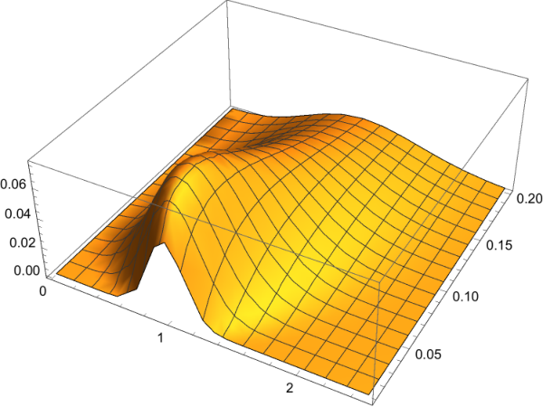
Figure 2: Plot of the spatio-temporal shape: mean local instantaneous velocity v⁡(z,t)=t−1​F​(z,1/t)v(z,t)=t^{-1}F(z,1/\sqrt{t}), i.e. Eq. (212) for z=ℓ2−x0ℓ2∈[0,2.5]z=\frac{\ell_{2}-x_{0}}{\ell_{2}}\in[0,2.5], and t∈[0,0.2]t\in[0,0.2]. We use units such that the seed-to-edge distance is ℓ2=1\ell_{2}=1. The mean velocity is larger near the seed at x0=xs=0x_{0}=x_{s}=0, i.e. z=1z=1. It vanishes exactly for all times on the edge of the avalanche, i.e. the line z=0z=0, as given in (217).

The spatiotemporal shape is defined by the instantaneous velocity, u˙​(x,t)\dot{u}(x,t), for an avalanche started at time t=0t=0 with its seed at x=0x=0. We study the mean spatiotemporal shape near an edge of the avalanche in Section V.2. To calculate the mean we will condition on a single edge, since it an easier calculation. We first compute the (cumulative) mean ⟨u˙​(x,t)⟩ℓ2<l2\langle\dot{u}(x,t)\rangle_{\ell_{2}<l_{2}} conditioned to the upper extension ℓ2\ell_{2} being smaller that l2l_{2}. It amounts to compute the euclidean Green function of a quantum particle in a 1/x21/x^{2} potential, a well known textbook problem. We find

⟨u˙​(x,t)⟩ℓ2<l2=l2​(l2−x)2​t​I72​(l2​(l2−x)2​t)​e−l22+(l2−x)24​t\displaystyle\langle\dot{u}(x,t)\rangle_{\ell_{2}<l_{2}}=\frac{\sqrt{l_{2}(l_{2}-x)}}{2t}I_{\frac{7}{2}}(\frac{l_{2}(l_{2}-x)}{2t})e^{-\frac{l_{2}^{2}+(l_{2}-x)^{2}}{4t}} (47)

in terms of a modified Bessel function. Similarly we find that the mean spatiotemporal shape at fixed avalanche upper extension ℓ2\ell_{2} is given by the scaling form

⟨u˙​(x,t)⟩ℓ2=ℓ23t​F​(ℓ2−xℓ2,ℓ2t)\displaystyle\langle\dot{u}(x,t)\rangle_{\ell_{2}}=\frac{\ell_{2}^{3}}{t}F(\frac{\ell_{2}-x}{\ell_{2}},\frac{\ell_{2}}{\sqrt{t}}) (48)

where the spatiotemporal shape scaling function F⁡(z,r)F(z,r) is given in terms of Bessel functions in (213), and is plotted in Fig. 2. We find that the mean instantaneous local velocity vanishes with the distance to the edge of the avalanche, with the same exponent 33, as does the mean static shape. The associated amplitude 𝒜t{\cal A}_{t} now depends on time, and we obtain its exact time dependence

⟨u˙(x,t)⟩ℓ2≃𝒜t(l2−x),3𝒜t=1tC(tℓ22),C(τ)=e−14​τ5040​π​τ7/2\displaystyle\langle\dot{u}(x,t)\rangle_{\ell_{2}}\simeq{\cal A}_{t}\left(l_{2}-x\right){}^{3}\quad,\quad{\cal A}_{t}=\frac{1}{t}C(\frac{t}{\ell_{2}^{2}})\quad,\quad C(\tau)=\frac{e^{-\frac{1}{4\tau}}}{5040\sqrt{\pi}\tau^{7/2}} (49)

As time increases, the amplitude 𝒜t{\cal A}_{t} reaches a maximum and then decays. One can check that by integration over time ∫0+∞d​t​𝒜t=∫0+∞d​ττ​C​(τ)=121\int_{0}^{+\infty}dt{\cal A}_{t}=\int_{0}^{+\infty}\frac{d\tau}{\tau}C(\tau)=\frac{1}{21} one recovers the universal static amplitude.

II.4 Higher dimension

The BFM in higher spatial dimension d>1d>1 is more complicated to analyze since the instanton equation admits fewer analytical solutions. However one can still obtain results about some properties of the support of the avalanche. We denote this support Ω⁡(xs)\Omega(x_{s}), where xsx_{s} is the position of the seed, and it consists in the set of points xx which have moved during the avalanche, i.e. with S⁡(x)>0S(x)>0. For the SR BFM that we are studying we can surmise that the avalanche is connected, but for d>1d>1 it can contain ”holes”. Our study is limited to the BFM in dimension d<4d<4. The observables that we study are illustrated in the Figure 3.

Refer to caption ​​​​​​​​​​​​ ​​​​​​​​​​​​ ​​​​​​​​​​​​ ​​​​​​​​​​​​ ​​​​​​​​​​​​

Figure 3: Schematic representation of the support of an avalanche for a 2-dimensional interface in the internal plane x=(x1,x2)x=(x_{1},x_{2}) (the direction of motion - not shown - being transverse to the plane of the figure). The region in blue is the support Ω\Omega, i.e. it contains all points that have moved (S⁡(x)>0S(x)>0). The region in white is the complementary, and contains all points that have not moved (S⁡(x)=0S(x)=0). The picture is a cartoon, as one rather expects a fractal structure. Here xsx_{s} is the position of the seed (the first point which moves). One studies here the following observables shown in the Figure: (i) the maximal distance reached by the avalanche rmaxr_{\rm max} (ii) the minimal distance of approach of a given point 00, rminr_{\rm\min} (iii) the total span ℓ\ell associated to a direction x1x_{1} as the ℓ=maxx∈Ω⁡(x1)−minx∈Ω⁡(x1)\ell=\max_{x\in\Omega}(x_{1})-\min_{x\in\Omega}(x_{1}), as well as the upper span ℓ2=maxx∈Ω⁡(x1)−xs\ell_{2}=\max_{x\in\Omega}(x_{1})-x_{s} and the lower span ℓ1=xs−minx∈Ω⁡(x1)\ell_{1}=x_{s}-\min_{x\in\Omega}(x_{1}).

II.4.1 Probability that a given point has not moved and mean shape around it

In Section VIII.1 we obtain the probability that a given point x0x_{0} does not belong to the support of the avalanche. It reads, for any d<4d<4

Prob⁡(S⁡(x0)=0)=Prob⁡(x0∉Ω⁡(xs))=e−f​2​(4−d)(x0−xs)2\displaystyle{\rm Prob}(S(x_{0})=0)={\rm Prob}(x_{0}\notin\Omega(x_{s}))=e^{-f\frac{2(4-d)}{(x_{0}-x_{s})^{2}}} (50)

Note that it means that either the avalanche maximal radius (studied below) is smaller than |xs−x0||x_{s}-x_{0}|, or (for d>1d>1) it is larger, and the point x0x_{0} belongs to a ”hole” inside the avalanche.

Now we can compute some observables conditioned to the event that S⁡(x0)=0S(x_{0})=0. The first one is the PDF of the variable Σ=∫dd​x​S⁡(x)(x−x0)4\Sigma=\int d^{d}x\frac{S(x)}{(x-x_{0})^{4}}. It turns out that this variable is finite and its PDF is obtained in (456). It exhibits a Σ−3/2\Sigma^{-3/2} power law regime, reminiscent of the one for the total size SS, with some cutoffs (see discussion there).

The second observable is the mean shape ⟨S⁡(x)⟩S⁡(x0)=0\langle S(x)\rangle_{S(x_{0})=0} conditioned to S⁡(x0)=0S(x_{0})=0. It amounts to solve for the Green function of a Schrodinger problem in a 1/r21/r^{2} potential in dimension dd. The complete result in any dd is given in (480), and in d=2d=2 (which is simpler) it is given in (473). Note that in d=1d=1 this observable corresponds to the cumulative conditional shape with a single boundary, see (471). The most interesting property is that the shape vanishes near the point x0x_{0} as a power law of the distance with a quite non-trivial exponent bd+b_{d}^{+} (we have chosen x0=0x_{0}=0 and denote the radial coordinates around that point as r=|x|r=|x| and rs=|xs|r_{s}=|x_{s}|)

⟨S(x)⟩S⁡(0)=0≃r→0fCdrsbd−rbd+,bd±=12(2−d±d2−20​d+68)\displaystyle\langle S(x)\rangle_{S(0)=0}\simeq_{r\to 0}fC_{d}r_{s}^{b_{d}^{-}}\,r^{b_{d}^{+}}\quad,\quad b_{d}^{\pm}=\frac{1}{2}\left(2-d\pm\sqrt{d^{2}-20d+68}\right) (51)

where CdC_{d} is a dimension dependent constant and with b2+=2​2b_{2}^{+}=2\sqrt{2}, b3+=12​(17−1)b_{3}^{+}=\frac{1}{2}(\sqrt{17}-1) and bd+→0b_{d}^{+}\to 0 as d→4−d\to 4^{-} (and one recovers b1+=4b_{1}^{+}=4 as found in d=1d=1).

II.4.2 Maximal distance reached by an avalanche and minimal distance of its support to a point

Let us define the maximal radius of an avalanche as rmax=maxx∈Ω⁡(xs)⁡|x−xs|r_{\max}=\max_{x\in\Omega(x_{s})}|x-x_{s}| the maximal distance that it reaches counted from the seed, see Figure 3. It is a random variable and we obtain in Section VIII.4 its CDF and its density, which read

Prob(rmax<R)=e−cdf/R2,ρ(rmax)=2​cdrmax3{\rm Prob}(r_{\max}<R)=e^{-c_{d}f/R^{2}}\quad,\quad\rho(r_{\max})=\frac{2c_{d}}{r_{\max}^{3}} (52)

with cd=2≈12.5634c_{d=2}\approx 12.5634, cd=3≈15.7179c_{d=3}\approx 15.7179. In d=1d=1 this observable identifies with Prob⁡(ℓ1<R,ℓ2<R){\rm Prob}(\ell_{1}<R,\ell_{2}<R) and one finds c1=32​𝒫0​(12,Γ​(1/3)18/(64​π6))=8.8475159..c_{1}=\frac{3}{2}{\cal P}_{0}(\frac{1}{2},\Gamma(1/3)^{18}/(64\pi^{6}))=8.8475159...

Another interesting observable is the minimal distance of approach, i.e. rmin=minx∈Ω⁡(xs)⁡|x|r_{\min}=\min_{x\in\Omega(x_{s})}|x|, 0<rmin<rs=|xs|0<r_{\min}<r_{s}=|x_{s}|, the minimal distance between the origin x=0x=0 and any point of the avalanche (started at xsx_{s}), see Figure 3. We denote its PDF as Prs​(rmin)P_{r_{s}}(r_{\min}). Of course, we know from (50) that there is a non zero probability, equal to p0=1−e−2​(4−d)​frs2p_{0}=1-e^{-\frac{2(4-d)f}{r_{s}^{2}}}, that rmin=0r_{\min}=0, i.e. that the point x=0x=0 belongs to the avalanche. So Prs​(rmin)P_{r_{s}}(r_{\min}) has a delta function piece p0​δ​(rs)p_{0}\delta(r_{s}) at zero. We have calculated Prs​(rmin)P_{r_{s}}(r_{\min}) in (506), (507). Let us indicate here only the behavior of the associated density ρrs​(rmin=R)=∂fPrs​(rmin=R)|f=0+\rho_{r_{s}}(r_{\min}=R)=\partial_{f}P_{r_{s}}(r_{\min}=R)|_{f=0^{+}} when rmin≪rsr_{\min}\ll r_{s}

ρrs​(rmin=R)≃BdR3+bd−​rs−bd−,0<rmin≪rs\rho_{r_{s}}(r_{\min}=R)\simeq\frac{B_{d}}{R^{3+b_{d}^{-}}r_{s}^{-b_{d}^{-}}}\quad,\quad 0<r_{\min}\ll r_{s} (53)

where BdB_{d} is a dimension dependent constant, and the exponent bd−b_{d}^{-} is defined in (51). Note that 3+bd−≥03+b_{d}^{-}\geq 0 and increases from 00 to 11 as dd increases from d=1d=1 to d=4d=4.

II.4.3 Probability of not hitting a cone in two dimension

Refer to caption ​​​​​​​​​​​​ ​​​​​​​​​​​​ ​​​​​​​​​​​​ ​​​​​​​​​​​​ ​​​​​​​​​​​​

Figure 4: Avalanche of seed xsx_{s} and support Ω\Omega (in blue) in two dimensions. We obtain the probability that it remains confined within the conical domain of apex in 00 and opening angle ϕ0\phi_{0}, as represented schematically. For ϕ0=π\phi_{0}=\pi it is related to the distribution of ℓ1\ell_{1} defined in Fig. 3. For ϕ0→2​π\phi_{0}\to 2\pi it becomes the probability that the avalanche does not intersect the positive half-axis.

Consider the conical domain in d=2d=2, in polar coordinates 𝒟=(r,ϕ)∈]0,+∞[×]0,ϕ0[{\cal D}=(r,\phi)\in]0,+\infty[\times]0,\phi_{0}[ with an opening angle 0<ϕ0≤2​π0<\phi_{0}\leq 2\pi. We ask what is the probability that an avalanche Ω⁡(xs)\Omega(x_{s}), with a seed inside the wedge at x=(rs,ϕs)x=(r_{s},\phi_{s}), remains strictly confined inside the wedge (i.e. is not allowed to touch the two radial lines at ϕ=0,ϕ0\phi=0,\phi_{0}). We find in Section VIII.6 that it equals

Prob(S(r,0)=S(r,ϕ0)=0,∀r∈[0,+∞[)=exp(−6​frs2(13+hϕ0(ϕs))){\rm Prob}(S(r,0)=S(r,\phi_{0})=0,\forall r\in[0,+\infty[)=\exp\left(-\frac{6f}{r_{s}^{2}}(\frac{1}{3}+h_{\phi_{0}}(\phi_{s}))\right) (54)

where hϕ0​(ϕ)h_{\phi_{0}}(\phi) is a Weierstrass function with parameter g3=g3​(ϕ0)g_{3}=g_{3}(\phi_{0}) determined by the condition that its period, denoted 2​Ω​(43,g3)2\Omega(\frac{4}{3},g_{3}), equals ϕ0\phi_{0}, namely

hϕ0(ϕ)=𝒫(ϕ;g2=43,g3(ϕ0)),g3=g3(ϕ0)⇔2Ω(43,g3)=2∫e1+∞d​t4​t3−43​t−g3=ϕ0h_{\phi_{0}}(\phi)={\cal P}(\phi;g_{2}=\frac{4}{3},g_{3}(\phi_{0}))\quad,\quad g_{3}=g_{3}(\phi_{0})\quad\Leftrightarrow\quad 2\Omega(\frac{4}{3},g_{3})=2\int_{e_{1}}^{+\infty}\frac{dt}{\sqrt{4t^{3}-\frac{4}{3}t-g_{3}}}=\phi_{0} (55)

where t=e1t=e_{1} is the largest positive root of 4​t3−43​t−g3=04t^{3}-\frac{4}{3}t-g_{3}=0, a condition equivalent to asking that 𝒫′​(ϕ0/2,g2=43,g3​(ϕ0))=0{\cal P}^{\prime}(\phi_{0}/2;g_{2}=\frac{4}{3},g_{3}(\phi_{0}))=0. One finds that g3g_{3} decreases as ϕ0\phi_{0} increases, with g3∈[g3c,+∞[g_{3}\in[g_{3}^{c},+\infty[, where g3≃g30/ϕ06g_{3}\simeq g_{3}^{0}/\phi_{0}^{6} for a small cone opening angle ϕ0≪1\phi_{0}\ll 1 and g3c≈−0.295402g_{3}^{c}\approx-0.295402 corresponds to ϕ0=2​π\phi_{0}=2\pi, i.e. the probability that the avalanche does not intersect the positive half axis.

From these results, we also obtain in Eq. (559) the joint CDF of the ”angular extensions” φ2=maxx=(r,ϕ)∈Ω⁡ϕ\varphi_{2}=\max_{x=(r,\phi)\in\Omega}\phi and φ1=−minx=(r,ϕ)∈Ω⁡ϕ\varphi_{1}=-\min_{x=(r,\phi)\in\Omega}\phi (for ϕs=0\phi_{s}=0), i.e. the angular analogs of ℓ1,ℓ2\ell_{1},\ell_{2}, as well as the PDF of the total angular extension φ=φ1+φ2\varphi=\varphi_{1}+\varphi_{2} by differentiation.

II.4.4 Avalanche span and shape in d>1d>1

In dimension dd, as we discussed above, one can define the span ℓ\ell of the avalanche along one given axis, say x1x_{1}, and the distances ℓ1\ell_{1} and ℓ2\ell_{2} from the seed to the lines (in general hyperplanes) as defined in the caption of Fig. 3.

With this definition we know that all joint statistics of ℓ1,ℓ2\ell_{1},\ell_{2} and St​o​t​(x1)=∫dd−1​x⟂​S​(x1,x⟂)S_{tot}(x_{1})=\int d^{d-1}x_{\perp}S(x_{1},x_{\perp}) is identical to the one for the d=1d=1 BFM that we have already calculated. For instance, the mean shape integrated over the transverse space x⟂x_{\perp}, ⟨St​o​t​(x1)⟩ℓ\langle S_{tot}(x_{1})\rangle_{\ell}, is given by the same formula.

One can also ask about the local mean shape at a point, ⟨S⁡(x1,x⟂)⟩ℓ\langle S(x_{1},x_{\perp})\rangle_{\ell}, i.e. not integrated. It is a related but different question which contains non trivial information also in the transverse direction. This is studied in Section (VIII.5), where we obtain the following result

⟨S⁡(x1,x⟂)⟩ℓ2<l2=f​∫dd−1​q(2​π)d−1​ei​q​(x⟂−x⟂s)​F|q|​(l2+x1s−x1,l2)\displaystyle\langle S(x_{1},x_{\perp})\rangle_{\ell_{2}<l_{2}}=f\int\frac{d^{d-1}q}{(2\pi)^{d-1}}e^{iq(x_{\perp}-x^{s}_{\perp})}F_{|q|}(l_{2}+x_{1}^{s}-x_{1},l_{2}) (56)
Fq​(a,b)=a​b​(I7/2​(q​a)​K7/2​(q​b)​θ​(0<a<b)+K7/2​(q​a)​I7/2​(q​b)​θ​(0<b<a))\displaystyle F_{q}(a,b)=\sqrt{ab}\big(I_{7/2}(qa)K_{7/2}(qb)\theta(0<a<b)+K_{7/2}(qa)I_{7/2}(qb)\theta(0<b<a)\big)

in terms of modified Bessel functions. If one integrates this equation over x⟂x_{\perp}, it selects q=0q=0, in which limit one has Fq→0​(a,b)=a47​b3​θ​(0<a<b)+b47​a3​θ​(0<b<a)F_{q\to 0}(a,b)=\frac{a^{4}}{7b^{3}}\theta(0<a<b)+\frac{b^{4}}{7a^{3}}\theta(0<b<a), recovering (24) and (25) as expected (see discussion above).

One obtains similarly the mean shape at fixed upper span ℓ2\ell_{2}. We display its expression in d=2d=2, choosing the origin xs=(x1s,x⟂s)=0x_{s}=(x_{1}^{s},x_{\perp}^{s})=0 as the position of the seed

⟨S⁡(y1,y⟂)⟩ℓ2=ℓ2​(2​ℓ2−y1)24​(2​π)​(ℓ2−y1)2​(y12+y⟂2)​Σ​(y12+y⟂22​ℓ2​(ℓ2−y1))\displaystyle\langle S(y_{1},y_{\perp})\rangle_{\ell_{2}}=\frac{\ell_{2}(2\ell_{2}-y_{1})}{24(2\pi)(\ell_{2}-y_{1})^{2}}\,(y_{1}^{2}+y_{\perp}^{2})\,\Sigma\left(\frac{y_{1}^{2}+y_{\perp}^{2}}{2\ell_{2}(\ell_{2}-y_{1})}\right) (57)
Σ⁡(z)=(z+1)​(15​z​(z+2)+2)2​z​(z+2)−34​(5​z​(z+2)+4)​log⁡(1+2z)\displaystyle\Sigma(z)=\frac{(z+1)(15z(z+2)+2)}{2z(z+2)}-\frac{3}{4}(5z(z+2)+4)\log(1+\frac{2}{z}) (58)

From the asymptotics of the scaling function Σ⁡(z)\Sigma(z), one finds again that the mean shape vanishes near the upper edge with a cubic power, but with an amplitude which decreases with |x⟂||x_{\perp}|, the transverse distance to the seed, on a scale ℓ2\ell_{2}, and with a high power, as 1/|x⟂|81/|x_{\perp}|^{8}, more precisely

⟨S⁡(x1,x⟂)⟩ℓ2=16​ℓ27105​π​(ℓ22+x⟂2)4​(ℓ2−x1)3+O⁡((ℓ2−x1)4)\langle S(x_{1},x_{\perp})\rangle_{\ell_{2}}=\frac{16\ell_{2}^{7}}{105\pi\left(\ell_{2}^{2}+x_{\perp}^{2}\right)^{4}}\,(\ell_{2}-x_{1})^{3}+O((\ell_{2}-x_{1})^{4}) (59)

Integration of the amplitude of the cubic power over x⟂x_{\perp} recovers the universal coefficient 121\frac{1}{21}. So, for a given position of the seed, there is a non-trivial shape structure in the transverse direction near the edge of the avalanche.

II.5 Tip driving PDF of local and total sizes, extension distribution and spatial shape

We now consider driving by the tip, as described in Section I.3, and focus on d=1d=1. The equation of motion is (18) contains two mass scales, a local one, m02m_{0}^{2}, equal to the curvature of the local well which drives u⁡(x=0,t)u(x=0,t) and a uniform mass m2m^{2} which, when present, acts as a cutoff for large avalanches. We study the avalanche produced by the driving kick at x=0x=0, f⁡(x,t)=δ⁡(x)​m02​w​δ​(t)f(x,t)=\delta(x)m_{0}^{2}w\delta(t) in (18).

We first present the results for m=0m=0. Since L^m0=m0−2\hat{L}_{m_{0}}=m_{0}^{-2} has the dimension of a lenght scale (in the internal xx direction) a crossover occurs as m0m_{0} is varied. In the limit m0→0m_{0}\to 0 one recovers the results for ”imposed local force” driving, while for m0→+∞m_{0}\to+\infty we have ”imposed local displacement”. The crossover between the two was not studied in Delorme and is obtained here exactly. We obtain the joint PDF, Pw​(S,S0)P_{w}(S,S_{0}), of the total size SS, and of the local jump S0=S⁡(x=0)S_{0}=S(x=0) at the tip x=0x=0, and its marginal distributions, as a function of m0m_{0}. There is a crossover scale at S=S^m0S=\hat{S}_{m_{0}} for avalanche sizes, such that below and above this scale the avalanche look different

S≪S^m0⇔imposed local force\displaystyle S\ll\hat{S}_{m_{0}}\quad\Leftrightarrow\quad\text{imposed local force} (60)
S≫S^m0⇔imposed local displacement\displaystyle S\gg\hat{S}_{m_{0}}\quad\Leftrightarrow\quad\text{imposed local displacement} (61)

with, and similarly for the crossover scale in the local size at S0=S^m00S_{0}=\hat{S}^{0}_{m_{0}} (in units σ=η=1\sigma=\eta=1)

S^m0=m0−8,S^m00=m0−6\hat{S}_{m_{0}}=m_{0}^{-8}\quad,\quad\hat{S}^{0}_{m_{0}}=m_{0}^{-6} (62)

(noted with a hat to distinguish it from SmS_{m} the upper cutoff scale of avalanches in presence of a uniform mass). So large avalanches always feel the ”imposed displacement”. This scaling is expected, more generally one expects S^m0∼L^m0d+ζ\hat{S}_{m_{0}}\sim\hat{L}_{m_{0}}^{d+\zeta} and S0∼L^m0ζS_{0}\sim\hat{L}_{m_{0}}^{\zeta} with here ζ=ζBFM=3\zeta=\zeta_{\rm BFM}=3 and more generally d+ζBFM=4d+\zeta_{\rm BFM}=4. Note that in the limit m0→+∞m_{0}\to+\infty the local jump is exactly constrained,

II.5.1 Distribution of local jumps at the tip

Let us start with Pw​(S0)P_{w}(S_{0}), we find in Section VII.2.3

Pw​(S0)\displaystyle P_{w}(S_{0}) =\displaystyle= 131/3​S05/3​w​m02​e23​y3​(−y​Ai​(y2)−Ai′​(y2)),y=m02​(S0−w)2×31/3​S02/3\displaystyle\frac{1}{3^{1/3}S_{0}^{5/3}}wm_{0}^{2}\,e^{\frac{2}{3}y^{3}}(-y{\rm Ai}(y^{2})-{\rm Ai}^{\prime}(y^{2}))\quad,\quad y=\frac{m_{0}^{2}(S_{0}-w)}{2\times 3^{1/3}S_{0}^{2/3}} (63)

One can check that the first moment exists with ⟨S0⟩=w\langle S_{0}\rangle=w, and that in the limit m0→+∞m_{0}\to+\infty, Pw​(S0)P_{w}(S_{0}) converges to δ⁡(S0−w)\delta(S_{0}-w) as expected, since then the displacement is fully imposed. Note that at fixed ww, there is a cutoff for small avalanches S0min∼m03​w3/2S_{0}^{\min}\sim m_{0}^{3}w^{3/2}. From (63) one obtains the density ρ⁡(S0)=∂wPw​(S0)|w=0+\rho(S_{0})=\partial_{w}P_{w}(S_{0})|_{w=0^{+}} in (350), and one finds that exhibits the single crossover scale S0∼S^m0=m0−6S_{0}\sim\hat{S}_{m_{0}}=m_{0}^{-6}. Using Airy function asymptotics (see (353)) one finds that the density crosses over between the two power laws characteristic respectively of the force imposed and the displacement imposed regimes

ρ⁡(S0)≃m0232/3​Γ​(13)​S05/3,S0≪S^m0=m0−6\displaystyle\rho(S_{0})\simeq\frac{m_{0}^{2}}{3^{2/3}\Gamma(\frac{1}{3})S_{0}^{5/3}}\quad,\quad S_{0}\ll\hat{S}_{m_{0}}=m_{0}^{-6} (64)
ρ⁡(S0)≃32​π​1m03​S05/2,S0≫S^m0=m0−6\displaystyle\rho(S_{0})\simeq\sqrt{\frac{3}{2\pi}}\frac{1}{m_{0}^{3}S_{0}^{5/2}}\quad,\quad S_{0}\gg\hat{S}_{m_{0}}=m_{0}^{-6} (65)

and our result (350) describes the full crossover. The first limiting case (force imposed) (64) was already obtained in Delorme but the behavior (65) is new. Note however that it holds only in some regime at finite m0m_{0}, since for m0=+∞m_{0}=+\infty the displacement at the tip is fixed by the driving and equal to S0=wS_{0}=w. This crossover is discussed in Section VII.2.3.

II.5.2 Distribution of total sizes

The distribution of the total size SS of the avalanche, Pw​(S)P_{w}(S), is obtained in Section (VII.2.2) in the Laplace transform form (339). On this form one shows that it exhibits a crossover between two limits. For S≪S^m0S\ll\hat{S}_{m_{0}}, equivalently for m0→0m_{0}\to 0 at fixed S,wS,w

Pw​(S)=m02​w​e−m04​w24​S2​π​S3/2\displaystyle P_{w}(S)=\frac{m_{0}^{2}we^{-\frac{m_{0}^{4}w^{2}}{4S}}}{2\sqrt{\pi}S^{3/2}} (66)

which is normalized to unity. It is exactly the massless limit Pf​(S)=f​e−f24​S2​π​S3/2P_{f}(S)=\frac{fe^{-\frac{f^{2}}{4S}}}{2\sqrt{\pi}S^{3/2}} of the standard size distribution with driving at imposed force f=∫d​x​𝑑t​m02​w​δ​(t)​δ​(x)f=\int dxdtm_{0}^{2}w\delta(t)\delta(x). In the opposite limit S≫S^m0S\gg\hat{S}_{m_{0}}, equivalently m02→+∞m_{0}^{2}\to+\infty at fixed S,wS,w, we obtain

Pw​(S)=L​Tp→S−1​e−w​23​(4​p)3/4=32/3(4​w)4/3​ℒ3/4​(32/3​S/(4​w)4/3)\displaystyle P_{w}(S)=LT^{-1}_{p\to S}e^{-w\sqrt{\frac{2}{3}}(4p)^{3/4}}=\frac{3^{2/3}}{(4w)^{4/3}}{\cal L}_{3/4}(3^{2/3}S/(4w)^{4/3}) (67)

with ℒ3/4{\cal L}_{3/4} being the stable Levy law of index 3/43/4, see Appendix B where its explicit expression is given in terms of hypergeometric functions. The associated size density ρ(S)=∂w|w=0+Pw(S)\rho(S)=\partial_{w}|_{w=0^{+}}P_{w}(S) has the explicit expression

ρ⁡(S)=3Γ⁡(1/4)​S7/4\displaystyle\rho(S)=\frac{\sqrt{3}}{\Gamma(1/4)S^{7/4}} (68)

which was also found in Delorme.

II.5.3 Joint distribution of total size and of local jump at the tip

Although it is not easy to obtain directly an explicit expression for the full crossover form Pw​(S)P_{w}(S), we have able to obtain the explicit expression of the JPDF Pw​(S,S0)P_{w}(S,S_{0}) for both the massive and massless cases in Section VII.2.4. The result is bulky and displayed in (365). Here we show only its associated density, ρ(S,S0)=∂w|w=0Pw(S,S0)\rho(S,S_{0})=\partial_{w}|_{w=0}P_{w}(S,S_{0}), and for the massless case m2=0m^{2}=0. It takes the scaling form

ρ⁡(S,S0)=m020​ρ^​(m08​S,m06​S0)\rho(S,S_{0})=m_{0}^{20}\hat{\rho}(m_{0}^{8}S,m_{0}^{6}S_{0}) (69)

where the scaling function reads

ρ^​(S,S0)=2 32/3​S01/3​exp⁡(−3​S03S2+S036−S022​S−6​S04S3)π​S5/2​(y​Ai​(y2)−Ai′​(y2)),y=S01/3​S+6​S02​33​S\displaystyle\hat{\rho}(S,S_{0})=\frac{2\ 3^{2/3}S_{0}^{1/3}\exp\left(-\frac{3S_{0}^{3}}{S^{2}}+\frac{S_{0}}{36}-\frac{S_{0}^{2}}{2S}-\frac{6S_{0}^{4}}{S^{3}}\right)}{\sqrt{\pi}S^{5/2}}\left(y\text{Ai}\left(y^{2}\right)-\text{Ai}^{\prime}\left(y^{2}\right)\right)\quad,\quad y=S_{0}^{1/3}\frac{S+6S_{0}}{2\sqrt[3]{3}S} (70)

Finally, note that we have also given the lowest moments of S,S0S,S_{0} and joint moments in the massive case in Section VII.2.1.

II.5.4 Distributions of extensions for tip-driven avalanches

In tip-driven avalanches the seed is always at xs=x=0x_{s}=x=0. One is thus interested in the distribution of ℓ2\ell_{2} the distance of the seed to the upper edge at x=ℓ2x=\ell_{2}. In Section VII.3 we obtain its CDF as

Prob⁡(ℓ2<r)=e−6​m06​w​ϕ​(r​m02)\displaystyle{\rm Prob}(\ell_{2}<r)=e^{-6m_{0}^{6}w\,\phi(rm_{0}^{2})} (71)

where the function ϕ⁡(r)\phi(r) is defined by inversion

ϕ=ϕ(r)⇔r=∫ϕ+∞d​y4​y3+ϕ2+4​ϕ5/2=2F1(16,12;76;−ϕ2+4​ϕ5/24​ϕ3)1ϕ\displaystyle\phi=\phi(r)\quad\Leftrightarrow\quad r=\int_{\phi}^{+\infty}\frac{dy}{\sqrt{4y^{3}+\phi^{2}+4\phi^{5/2}}}=\,_{2}F_{1}\left(\frac{1}{6},\frac{1}{2};\frac{7}{6};-\frac{\phi^{2}+4\phi^{5/2}}{4\phi^{3}}\right)\frac{1}{\sqrt{\phi}} (72)

which can also be written as ϕ=𝒫⁡(r,0,g3=−ϕ2−4​ϕ5/2)\phi={\cal P}(r,0,g_{3}=-\phi^{2}-4\phi^{5/2}). The detailed asymptotics of ϕ⁡(r)\phi(r) and of the CDF are given in (378), (379) and (380). From the CDF one obtains the PDF P⁡(ℓ2)P(\ell_{2}) and the corresponding density, which reads

ρ(ℓ2)=∂w|w=0+P(ℓ2)=−6m08ϕ′(m02ℓ2)\displaystyle\rho(\ell_{2})=\partial_{w}|_{w=0^{+}}P(\ell_{2})=-6m_{0}^{8}\phi^{\prime}(m_{0}^{2}\ell_{2}) (73)

Its asymptotics are obtained in Section VII.3 as

ρ⁡(ℓ2)≃12​m02ℓ23,ℓ2≪m0−2\displaystyle\rho(\ell_{2})\simeq\frac{12m_{0}^{2}}{\ell_{2}^{3}}\quad,\quad\ell_{2}\ll m_{0}^{-2} (74)
ρ⁡(ℓ2)≃36​Γ​(13)3​Γ​(76)3π3/2​ℓ24=99.2466..ℓ24,ℓ2≫m0−2\displaystyle\rho(\ell_{2})\simeq\frac{36\Gamma\left(\frac{1}{3}\right)^{3}\Gamma\left(\frac{7}{6}\right)^{3}}{\pi^{3/2}\ell_{2}^{4}}=\frac{99.2466..}{\ell_{2}^{4}}\quad,\quad\ell_{2}\gg m_{0}^{-2} (75)

The first regime of small ℓ2\ell_{2} also corresponds to the limit of small m0m_{0}, i.e. m0→0m_{0}\to 0, and one recover ρf(ℓ2)=∂f|f=0+P(ℓ2)≃12ℓ23\rho_{f}(\ell_{2})=\partial_{f}|_{f=0^{+}}P(\ell_{2})\simeq\frac{12}{\ell_{2}^{3}}, i.e. (23), the result (for a single boundary) in the regime of ”imposed local force” f=m02​wf=m_{0}^{2}w. The second regime, of large extension ℓ2\ell_{2}, also corresponds to the limit of large m0m_{0}, i.e. m0→+∞m_{0}\to+\infty: it is the regime of ”imposed local position” and leads to a new result, with a different decay exponent, ρ⁡(ℓ2)∼1/ℓ24\rho(\ell_{2})\sim 1/\ell_{2}^{4}.

Now, for finite m0m_{0} the upper extension ℓ2\ell_{2} and the lower one ℓ1\ell_{1} will be correlated non-trivially. In the limit m0→+∞m_{0}\to+\infty of strict imposed displacement, however, they become two independent random variables. We now study the avalanche shape in this limit.

II.5.5 Mean shape of a tip-driven avalanche and its fluctuations near the edge

We have obtained in Section VII.4.2 the mean shape of an avalanche of a given extension ℓ2\ell_{2}, in the limit m0→+∞m_{0}\to+\infty of strict imposed displacement, for 0≤x≤r0\leq x\leq r

⟨S⁡(x)⟩ℓ2<r=w​𝗌>​(xr),𝗌>​(0)=1,𝗌>​(1)=0\displaystyle\langle S(x)\rangle_{\ell_{2}<r}=w\,{\sf s}_{>}(\frac{x}{r})\quad,\quad{\sf s}_{>}(0)=1\quad,\quad{\sf s}_{>}(1)=0 (76)
𝗌>​(z)=1𝒫′​(1,0,g3∗)​(2​𝒫​(1−z,0,g3∗)+(1−z)​𝒫′​(1−z,0,g3∗))\displaystyle{\sf s}_{>}(z)=\frac{1}{{\cal P}^{\prime}(1,0,g_{3}^{*})}(2{\cal P}(1-z,0,g_{3}^{*})+(1-z){\cal P}^{\prime}(1-z,0,g_{3}^{*})) (77)

where 𝒫′​(1,0,g3∗)=−(−g3∗)1/2{\cal P}^{\prime}(1,0,g_{3}^{*})=-(-g_{3}^{*})^{1/2} from the properties of the Weierstrass function, and g3∗=−4​Γ​(13)6​Γ​(76)6π3=−30.400905g_{3}^{*}=-\frac{4\Gamma\left(\frac{1}{3}\right)^{6}\Gamma\left(\frac{7}{6}\right)^{6}}{\pi^{3}}=-30.400905 is the negative root of the equation 𝒫⁡(1,0,g3)=0{\cal P}(1,0,g_{3})=0. The condition 𝗌>​(0)=1{\sf s}_{>}(0)=1 is correctly recovered, as it should since for strictly imposed displacement (limit m0→+∞m_{0}\to+\infty), at the tip S⁡(x=0)=wS(x=0)=w with no fluctuations. Near the edge of the avalanche

𝗌>(z)≃3​Γ​(13)3​Γ​(76)37​π3/2(1−z)4=1.18150748..×(1−z)4\displaystyle{\sf s}_{>}(z)\simeq\frac{3\Gamma\left(\frac{1}{3}\right)^{3}\Gamma\left(\frac{7}{6}\right)^{3}}{7\pi^{3/2}}(1-z)^{4}=1.18150748..\times(1-z)^{4} (78)

The mean shape conditioned to the extension ℓ2\ell_{2} is given by the exact formula (also compatible with S⁡(x=0)=wS(x=0)=w)

⟨S⁡(x)⟩ℓ2=w​𝗌>​(z)−wℓ2​P​(ℓ2)​z​𝗌>′​(z),z=xℓ2\displaystyle\langle S(x)\rangle_{\ell_{2}}=w{\sf s}_{>}(z)-\frac{w}{\ell_{2}P(\ell_{2})}z\,{\sf s}_{>}^{\prime}(z)\quad,\quad z=\frac{x}{\ell_{2}} (79)

which, in the limit of infinitesimal driving has the finite limit, for 0≤x≤ℓ20\leq x\leq\ell_{2}

⟨S⁡(x)⟩ℓ2=−1ℓ2​ρ​(ℓ2)​z​𝗌>′​(z)=ℓ23​𝗌~​(z),z=xℓ2\displaystyle\langle S(x)\rangle_{\ell_{2}}=-\frac{1}{\ell_{2}\rho(\ell_{2})}z{\sf s}^{\prime}_{>}(z)=\ell_{2}^{3}\,\tilde{\sf s}(z)\quad,\quad z=\frac{x}{\ell_{2}} (80)
𝗌~​(z)=16​g3∗​z​(2​(1−z)​𝒫​(1−z,0,g3∗)2+𝒫′​(1−z,0,g3∗))\displaystyle\tilde{\sf s}(z)=\frac{1}{6g_{3}^{*}}z(2(1-z){\cal P}(1-z,0,g_{3}^{*})^{2}+{\cal P}^{\prime}(1-z,0,g_{3}^{*})) (81)

It is plotted in Fig. 5 (note that there 𝗌⁡(y0)=𝗌~​(z=1−y0){\sf s}(y_{0})=\tilde{\sf s}(z=1-y_{0}) here). It vanishes near the tip (since w→0w\to 0) as

𝗌~​(z)=18​π3/2​zΓ​(16)3​Γ​(13)3+O⁡(z2)=0.0302277​z+O⁡(z2)\displaystyle\tilde{\sf s}(z)=\frac{18\pi^{3/2}z}{\Gamma\left(\frac{1}{6}\right)^{3}\Gamma\left(\frac{1}{3}\right)^{3}}+O\left(z^{2}\right)=0.0302277z+O(z^{2}) (82)

and near the edge z→1−z\to 1^{-} as

𝗌~​(z)=121​(1−z)3−121​(z−1)4+O⁡((z−1)9)\displaystyle\tilde{\sf s}(z)=\frac{1}{21}(1-z)^{3}-\frac{1}{21}(z-1)^{4}+O\left((z-1)^{9}\right) (83)

i.e. with the same cubic power and the same prefactor as for the force driven avalanches obtained in (35), a manifestation of the aforementioned universality of the edge behavior. More detailed series expansions are given in (420) and (421).

Integrating ∫0ℓd​x0\int_{0}^{\ell}dx_{0} one obtains the mean total size at fixed extension

⟨S⟩ℓ2=ℓ24​−ζ⁡(1,0,g3∗)18​g3∗=0.0022097287584​ℓ24\displaystyle\langle S\rangle_{\ell_{2}}=\ell_{2}^{4}\frac{-\zeta(1;0,g_{3}^{*})}{18g_{3}^{*}}=0.0022097287584\,\ell_{2}^{4} (84)

which is also obtained by an equivalent calculation in Section VII.4.4, together with the higher moments ⟨Sp⟩ℓ2\langle S^{p}\rangle_{\ell_{2}} in (445) and their generating function.


Figure 5: Left: Plot of the scaling function describing the mean shape of an avalanche with imposed displacement at the tip (m0=+∞m_{0}=+\infty). What is plotted is 𝗌⁡(y0)=s~​(z=1−y0){\sf s}(y_{0})=\tilde{s}(z=1-y_{0}) as a function of y0y_{0}. The mean shape vanishes with a cubic power at the edge of the avalanche y0=0y_{0}=0 (z=1z=1) and linearly at the driving tip y0=1y_{0}=1 (z=0z=0). Right: idem for the second shape (second moment of the shape), here is a plot of 𝗌2​(y0){\sf s}_{2}(y_{0}) defined in the text. It vanishes with the sixth power at the edge, and we show that the nn-th moment vanishes with power 3​n3n, with a prefactor that can be extracted from our general formula.

Figure 6: Plot of the ratio 𝗌2​(y0)/𝗌​(y0)2{\sf s}_{2}(y_{0})/{\sf s}(y_{0})^{2} for y0∈[0,1]y_{0}\in[0,1], with the same notations as in Fig. 5.

Second shape and full mean distribution near the edge. In Section VII.4.3 we calculate the second shape, that is ⟨S​(x)2⟩ℓ2\langle S(x)^{2}\rangle_{\ell_{2}}. It is given in the form ⟨S​(x)2⟩ℓ2=ℓ26​𝗌2​(1−xℓ2)\langle S(x)^{2}\rangle_{\ell_{2}}=\ell_{2}^{6}\,{\sf s}_{2}(1-\frac{x}{\ell_{2}}) where the scaling function 𝗌2​(y){\sf s}_{2}(y), 0≤y≤10\leq y\leq 1 is given in (428) and plotted in Fig. 5. The ratio ⟨S​(x)2⟩ℓ2⟨S⁡(x)⟩ℓ22\frac{\langle S(x)^{2}\rangle_{\ell_{2}}}{\langle S(x)\rangle_{\ell_{2}}^{2}} is plotted in Fig. 6, varies between 2113=1.61538\frac{21}{13}=1.61538 for xx near ℓ2\ell_{2}, as in (31), and 22 for xx near the tip x=0x=0. One finds that near the edge of the avalanche

⟨S​(x)2⟩ℓ2≃1273​(ℓ2−x)6\langle S(x)^{2}\rangle_{\ell_{2}}\simeq\frac{1}{273}(\ell_{2}-x)^{6} (85)

exactly the same leading order result, up to the amplitude, as for the force imposed avalanches. We show in Section VII.4.3 (see Remark about universality at the end) that for the tip driven avalanches, one can also write S⁡(x)≃σ×(ℓ2−x)3S(x)\simeq\sigma\times(\ell_{2}-x)^{3} near the edge, with the same probability distribution p⁡(σ)p(\sigma) for the random variable σ\sigma as given in (28), (29) (with lowest order moments given in (30)), which is thus universal (and reproduces all the moments of the shape near the edge).

III Method: generating function and instanton equation

In the BFM model (3) it is possible to express averages of exponentials of linear functions of the velocity field in terms of solutions of a non-linear partial differential equation, see Refs. DobrinevskiLeDoussalWiese2011b; LeDoussalWiese2012a for details. Since here we mostly study observables based on avalanche sizes, we mostly need the ”static” version of this property. It states that for an initial condition u˙​(x,t=0−)=0\dot{u}(x,t=0^{-})=0 and any forward driving f˙​(x,t)≥0\dot{f}(x,t)\geq 0, as well as any ”source” function λ⁡(x)\lambda(x) so that the l.h.s exists, one has

G⁡[λ⁡(x)]:=exp⁡(∫dd​x​λ​(x)​S​(x))¯=e∫dd​x​f​(x)​u~λ​(x).G[\lambda(x)]:=\overline{\exp\left(\int d^{d}x\lambda(x)S(x)\right)}=e^{\int d^{d}xf(x)\tilde{u}^{\lambda}(x)}\ . (86)

where here f⁡(x)=∫0+∞d​t​f˙​(x,t)f(x)=\int_{0}^{+\infty}dt\dot{f}(x,t). In this paper ⋯¯\overline{\cdots} denotes the average over the disorder, i.e. the Brownian random force field, equivalently over ξ⁡(x,t)\xi(x,t) in (3). The function u~λ​(x)\tilde{u}^{\lambda}(x) is the solution of the (time independent) ”instanton equation”

∇x2​u~​(x)−A​u~​(x)+u~​(x)2=−λ⁡(x).\nabla_{x}^{2}\tilde{u}(x)-A\tilde{u}(x)+\tilde{u}(x)^{2}=-\lambda(x)\ . (87)

where A=1A=1 for the massive case and A=0A=0 for the massless case, in the units defined in Section I.2.1 in each case.

To calculate the total avalanche size one needs a uniform source in the instanton equation: λ⁡(x)=λ\lambda(x)=\lambda, and for the local size we need a local source, i.e. in d=1d=1, λ⁡(x)=λ​δ​(x)\lambda(x)=\lambda\delta(x). To obtain information about the extension of the avalanches, we consider a source localized at two points in space, in d=1d=1, λ⁡(x)=λ1​δ​(x−r1)+λ2​δ​(x−r2)\lambda(x)=\lambda_{1}\delta(x-r_{1})+\lambda_{2}\delta(x-r_{2}).

The dynamical version of (86) and (87) is recalled when we need it in Section V.2 below. In Sections IV to VII we specialize to d=1d=1, and consider d>1d>1 in Section VIII.

IV Bulk driving: density of local size versus the distance to the seed

We study here various properties of the local size of an avalanche in d=1d=1. We use the dimensionless units. The Laplace transform (LT) of the PDF, P{f⁡(x)}​(S0)P_{\{f(x)\}}(S_{0}), of the local avalanche size S0=S⁡(x=0)S_{0}=S(x=0) following a kick (4) of amplitude f⁡(x)f(x) is given from (86) as

eλ​S0¯=∫d​S0​eλ​S0​P{f⁡(x)}​(S0)=e∫d​x​f​(x)​uλ​(x)\displaystyle\overline{e^{\lambda S_{0}}}=\int dS_{0}e^{\lambda S_{0}}P_{\{f(x)\}}(S_{0})=e^{\int dxf(x)u^{\lambda}(x)} (88)

where uλ​(x)u^{\lambda}(x) is the solution of the 1D equation (87)

u~′′​(x)−A​u~​(x)+u~​(x)2=−λ​δ​(x)\displaystyle\tilde{u}^{\prime\prime}(x)-A\tilde{u}(x)+\tilde{u}(x)^{2}=-\lambda\delta(x) (89)

which vanishes at ±∞\pm\infty, with A=0A=0 in the massless case and A=1A=1 in the massive case. The explicit solution reads (see e.g. Delorme and references therein)

u~λ​(x)=6​(1−zλ2)​e−|x|(1+zλ+(1−zλ)​e−|x|)2,A=1\displaystyle\tilde{u}^{\lambda}(x)=\frac{6(1-z_{\lambda}^{2})e^{-|x|}}{(1+z_{\lambda}+(1-z_{\lambda})e^{-|x|})^{2}}\quad,\quad A=1 (90)
u~λ(x)=−6(|x|+xλ)2,,A=0\displaystyle\tilde{u}^{\lambda}(x)=-\frac{6}{(|x|+x_{\lambda})^{2}}\quad,\quad\quad,\quad A=0 (91)

where, (A=0A=0) from the discontinuity of the derivative at x=0x=0, xλ3=−24λx_{\lambda}^{3}=-\frac{24}{\lambda}, and (A=1A=1), z=zλz=z_{\lambda} is the solution of

λ=3​z​(1−z2)\displaystyle\lambda=3z(1-z^{2}) (92)

whose branch is continuously connected to z=1z=1 for λ=0\lambda=0. Note that u~​(x=0)=32​(1−z2)\tilde{u}(x=0)=\frac{3}{2}(1-z^{2}) (A=1A=1) and u~(x=0)=−6/xλ2=31/32(−λ)2/3\tilde{u}(x=0)=-6/x_{\lambda}^{2}=\frac{3^{1/3}}{2}(-\lambda)^{2/3}.

IV.1 Massless case

In the massless case the general result reads, from (88) and (90)

P{f⁡(x)}(S0)=LT−λ→S0−1e−6∫dxf(x)λ2/3(|x|​(−λ)1/3+(24)1/3)2\displaystyle P_{\{f(x)\}}(S_{0})=LT^{-1}_{-\lambda\to S_{0}}e^{-6\int dxf(x)\frac{\lambda^{2/3}}{(|x|(-\lambda)^{1/3}+(24)^{1/3})^{2}}} (93)

where L​T−1LT^{-1} denotes the Laplace inversion, which can be obtained explicitly in a few cases. The first two are known LeDoussalWiese2008c; LeDoussalWiese2012a; Delorme, and we recall them for completeness, the third is new.

  • •

    Uniform kick f⁡(x)=ff(x)=f. Using ∫dxu~λ(x)=−12/xλ\int dx\tilde{u}^{\lambda}(x)=-12/x_{\lambda} we obtain

    P{f}(S0):=Pf(S0)=LT−λ→S0−1e−2×32/3(−λ)1/3f\displaystyle P_{\{f\}}(S_{0}):=P_{f}(S_{0})=LT^{-1}_{-\lambda\to S_{0}}e^{-2\times 3^{2/3}(-\lambda)^{1/3}f} (94)

    Denoting α=2×32/3​f\alpha=2\times 3^{2/3}f and introducing z:=(−λ)1/3z:=(-\lambda)^{1/3}, we can write

    S0​Pf​(S0)\displaystyle S_{0}P_{f}(S_{0}) =\displaystyle= ∫Cd​λ2​i​π​e−λ​S0​∂λe−α​(−λ)1/3=∫Cd​z2​i​π​eS0​z3​∂ze−α​z\displaystyle\int_{C}\frac{d\lambda}{2i\pi}e^{-\lambda S_{0}}\partial_{\lambda}e^{-\alpha(-\lambda)^{1/3}}=\int_{C}\frac{dz}{2i\pi}e^{S_{0}z^{3}}\partial_{z}e^{-\alpha z} (95)
    =\displaystyle= −α​Φ​(a,b,c)|a=3​S0,b=0,c=−α\displaystyle-\alpha\Phi(a,b,c)|_{a=3S_{0},b=0,c=-\alpha} (96)

    Following Appendix A of Delorme we have defined Φ⁡(a,b,c)\Phi(a,b,c), for a≠0a\neq 0, as

    Φ(a,b,c):=∫Cd​z2​i​πea​z33+b​z2+c​z=|a|−1/3e2​b33​a2−b​caAi(b2|a|4/3−c​sgn​(a)|a|1/3),\displaystyle\Phi(a,b,c):=\int_{C}\frac{dz}{2i\pi}e^{a\frac{z^{3}}{3}+bz^{2}+cz}=|a|^{-1/3}e^{\frac{2b^{3}}{3a^{2}}-\frac{bc}{a}}{\rm Ai}\!\left(\frac{b^{2}}{|a|^{4/3}}-\frac{c~{\rm sgn}(a)}{|a|^{1/3}}\right)\ , (97)

    in terms of the Airy function. Here and below CC generically denotes appropriate contours in the complex plane. As in Delorme, our use of inverse LT formula and change in variables therein are heuristic here and below, an approach validated by careful checks of the final formulae. This gives

    Pf​(S0)=2×31/3​fS04/3​Ai​(2×31/3​fS01/3)\displaystyle P_{f}(S_{0})=\frac{2\times 3^{1/3}f}{S_{0}^{4/3}}{\rm Ai}(\frac{2\times 3^{1/3}f}{S_{0}^{1/3}}) (98)

    correctly normalized to unity, using ∫0+∞d​y​Ai​(y)=1/3\int_{0}^{+\infty}dy{\rm Ai}(y)=1/3. One has the two limiting behaviors

    Pf​(S0)\displaystyle P_{f}(S_{0}) ≃\displaystyle\simeq 324​f3/4​e−4​23​f3/2S0π​S05/4,S0≪f3\displaystyle\frac{\sqrt[4]{\frac{3}{2}}f^{3/4}e^{-\frac{4\sqrt{\frac{2}{3}}f^{3/2}}{\sqrt{S_{0}}}}}{\sqrt{\pi}S_{0}^{5/4}}\quad,\quad S_{0}\ll f^{3} (99)
    ≃\displaystyle\simeq fρ(S0)+O(S0−5/3),S0≫f3,ρ(S0)=233​Γ​(23)​S04/3\displaystyle f\rho(S_{0})+O(S_{0}^{-5/3})\quad,\quad S_{0}\gg f^{3}\quad,\quad\rho(S_{0})=\frac{2}{\sqrt[3]{3}\Gamma\left(\frac{2}{3}\right)S_{0}^{4/3}} (100)

    where ρ⁡(S0)\rho(S_{0}) is the total density of local size, which exhibits the exponent 4/34/3.

  • •

    Local kick and local size at the point of the kick f⁡(x)=f​δ​(x)f(x)=f\delta(x), and we recall, S0=S⁡(x=0)S_{0}=S(x=0). Using that u~(x=0)=−6/xλ2=−31/32(−λ)2/3\tilde{u}(x=0)=-6/x_{\lambda}^{2}=-\frac{3^{1/3}}{2}(-\lambda)^{2/3}

    P{f​δ​(x)}​(S0)=L​T−λ→S0−1​e−31/32​(−λ)2/3​f\displaystyle P_{\{f\delta(x)\}}(S_{0})=LT^{-1}_{-\lambda\to S_{0}}e^{-\frac{3^{1/3}}{2}(-\lambda)^{2/3}f} (101)

    Denoting α=31/32​f\alpha=\frac{3^{1/3}}{2}f and introducing z:=(−λ)1/3z:=(-\lambda)^{1/3} we can write

    S0​P{f​δ​(x)}​(S0)\displaystyle S_{0}P_{\{f\delta(x)\}}(S_{0}) =\displaystyle= ∫Cd​λ2​i​π​e−λ​S0​∂λe−α​(−λ)2/3=∫Cd​z2​i​π​eS0​z3​∂ze−α​z2\displaystyle\int_{C}\frac{d\lambda}{2i\pi}e^{-\lambda S_{0}}\partial_{\lambda}e^{-\alpha(-\lambda)^{2/3}}=\int_{C}\frac{dz}{2i\pi}e^{S_{0}z^{3}}\partial_{z}e^{-\alpha z^{2}} (102)
    =\displaystyle= −2α∂cΦ(a,b,c)|a=3​S0,b=−α,c=0\displaystyle-2\alpha\partial_{c}\Phi(a,b,c)|_{a=3S_{0},b=-\alpha,c=0} (103)

    leading to

    P{f​δ​(x)}​(S0)=f​e−f336​S0233​S05/3​(y​Ai​(y2)−Ai′​(y2)),y=f2×31/3​S02/3\displaystyle P_{\{f\delta(x)\}}(S_{0})=\frac{fe^{-\frac{f^{3}}{36S_{0}^{2}}}}{\sqrt[3]{3}S_{0}^{5/3}}(y{\rm Ai}(y^{2})-{\rm Ai}^{\prime}(y^{2}))\quad,\quad y=\frac{f}{2\times 3^{1/3}S_{0}^{2/3}} (104)

    The associated density exhibits the exponent 5/35/3 and reads

    ρ0​(S0)=132/3​Γ​(13)​S05/3\displaystyle\rho_{0}(S_{0})=\frac{1}{3^{2/3}\Gamma(\frac{1}{3})S_{0}^{5/3}} (105)
  • •

    Local kick, and local size at the point at a distance |xs||x_{s}| from the kick

    The formula for the PDF of the local jump at x=0x=0, S0=S⁡(x=0)S_{0}=S(x=0), for a kick at x=xsx=x_{s}, can be written as above as a contour integral by introducing z:=(−λ)1/3z:=(-\lambda)^{1/3}

    S0​P{f​δ​(x−xs)}​(S0)=∫Cd​z2​i​π​eS0​z3​∂ze−6​f​z2(|xs|​z+(24)1/3)2=3​S0​∫Cd​z2​i​π​eS0​z3​z2​e−6​f​z2(|xs|​z+(24)1/3)2\displaystyle S_{0}P_{\{f\delta(x-x_{s})\}}(S_{0})=\int_{C}\frac{dz}{2i\pi}e^{S_{0}z^{3}}\partial_{z}e^{-6f\frac{z^{2}}{(|x_{s}|z+(24)^{1/3})^{2}}}=3S_{0}\int_{C}\frac{dz}{2i\pi}e^{S_{0}z^{3}}z^{2}e^{-6f\frac{z^{2}}{(|x_{s}|z+(24)^{1/3})^{2}}} (106)

    A simpler expression can be obtained for the density. Note that there is now a non-zero probability that the avalanche started at xsx_{s} has not reached x=0x=0. The probability that x=0x=0 has moved is

    pf=1−ef​u~λ=−∞​(xs)=−fu~λ=−∞(xs)+O(f2),u~λ=−∞(xs)=−6/xs2p_{f}=1-e^{f\tilde{u}^{\lambda=-\infty}(x_{s})}=-f\tilde{u}^{\lambda=-\infty}(x_{s})+O(f^{2})\quad,\quad\tilde{u}^{\lambda=-\infty}(x_{s})=-6/x_{s}^{2} (107)

    hence one can write

    Pf​δ​(x−xs)​(S0)=(1−pf)​δ​(S0)+pf​P~f​δ​(x−xs)​(S0)\displaystyle P_{f\delta(x-x_{s})}(S_{0})=(1-p_{f})\delta(S_{0})+p_{f}\tilde{P}_{f\delta(x-x_{s})}(S_{0}) (108)

    where the regular part, P~\tilde{P}, is also normalized to unity, ∫S0>0P~f​δ​(x−xs)​(S0)=1\int_{S_{0}>0}\tilde{P}_{f\delta(x-x_{s})}(S_{0})=1. We obtain the density by expanding in ff for fixed S0>0S_{0}>0 as in (10) (which gets rid of a δ⁡(S0)\delta(S_{0}) piece which does not enter in the density). Taking a derivative w.r.t. ff of (106) we have

    ρxs​(S0)\displaystyle\rho_{x_{s}}(S_{0}) =\displaystyle= −18∫Cd​z2​i​πeS0​z3z4(|xs|​z+(24)1/3)2=−18∫0+∞tdt∫Cd​z2​i​πz4eS0​z3−t⁡(|xs|​z+(24)1/3)\displaystyle-18\int_{C}\frac{dz}{2i\pi}e^{S_{0}z^{3}}\frac{z^{4}}{(|{x_{s}}|z+(24)^{1/3})^{2}}=-18\int_{0}^{+\infty}tdt\int_{C}\frac{dz}{2i\pi}z^{4}e^{S_{0}z^{3}-t(|{x_{s}}|z+(24)^{1/3})} (109)
    =\displaystyle= −18∫0+∞tdte−t​(24)1/3∂b2Φ(a,b,c)|a=3​S0,b=0,c=−t​|xs|\displaystyle-18\int_{0}^{+\infty}tdte^{-t(24)^{1/3}}\partial_{b}^{2}\Phi(a,b,c)|_{a=3S_{0},b=0,c=-t|{x_{s}}|} (110)
    =\displaystyle= 4×31/3S05/3∫0+∞tdte−2×31/3t(12(t​|xs|31/3​S01/3)2Ai(t​|xs|31/3​S01/3)+Ai′(t​|xs|31/3​S01/3))\displaystyle\frac{4\times 3^{1/3}}{S_{0}^{5/3}}\int_{0}^{+\infty}tdte^{-2\times 3^{1/3}t}(\frac{1}{2}(\frac{t{|x_{s}|}}{3^{1/3}S_{0}^{1/3}})^{2}{\rm Ai}(\frac{t{|x_{s}|}}{3^{1/3}S_{0}^{1/3}})+{\rm Ai}^{\prime}(\frac{t{|x_{s}|}}{3^{1/3}S_{0}^{1/3}})) (111)

    It can be put in a scaling form

    ρxs​(S0)\displaystyle\rho_{x_{s}}(S_{0}) =\displaystyle= 1S05/3​ϕ​(S0|xs|3)\displaystyle\frac{1}{S_{0}^{5/3}}\phi(\frac{S_{0}}{|{x_{s}}|^{3}}) (112)
    ϕ⁡(s)\displaystyle\phi(s) =\displaystyle= −12s2/3∫0+∞dte−2×32/3ts1/3dd​t(t22Ai′(t))\displaystyle-12s^{2/3}\int_{0}^{+\infty}dte^{-2\times 3^{2/3}ts^{1/3}}\frac{d}{dt}(\frac{t^{2}}{2}{\rm Ai}^{\prime}(t)) (113)
    =\displaystyle= −12×32/3s∫0+∞dtt2e−2×32/3ts1/3Ai′(t)\displaystyle-12\times 3^{2/3}s\int_{0}^{+\infty}dtt^{2}e^{-2\times 3^{2/3}ts^{1/3}}{\rm Ai}^{\prime}(t) (114)

    This integral can be carried out exactly leading to

    ϕ⁡(s)=31/6​6π​s​e−24​s​(4​(18​s−1)​(2​s1/3​Γ​(13)​E43​(−24​s)−32/3​Γ​(53)​E53​(−24​s))CLOSE\displaystyle\phi(s)=\frac{3^{1/6}6}{\pi}se^{-24s}\bigg(4(18s-1)\big(2s^{1/3}\Gamma(\frac{1}{3})E_{\frac{4}{3}}(-24s)-3^{2/3}\Gamma(\frac{5}{3})E_{\frac{5}{3}}(-24s)\big) (115)
    OPEN+3​e24​s​(2​s1/3​Γ​(13)−32/3​Γ​(53)))\displaystyle~~~~~~~~~~~~~~~~~~~~~~~~~~~~+3e^{24s}\big(2s^{1/3}\Gamma(\frac{1}{3})-3^{2/3}\Gamma(\frac{5}{3})\big)\bigg) (116)

    where En​(z)=∫1+∞e−z​t​𝑑t/tnE_{n}(z)=\int_{1}^{+\infty}e^{-zt}dt/t^{n} is the exponential integral. Using that Ai′(0)=−1/(31/3Γ(1/3)){\rm Ai}^{\prime}(0)=-1/(3^{1/3}\Gamma(1/3)) and ∫0+∞dtt2Ai′(t)=32/3/Γ(−2/3)\int_{0}^{+\infty}dtt^{2}{\rm Ai}^{\prime}(t)=3^{2/3}/\Gamma(-2/3) one can write respectively the large and small ss asymptotics

    ϕ⁡(s)=132/3​Γ​(13)−(1s)2/3​Γ​(13)4​(35/6​π)+5​Γ​(23)36​36​π​s+O⁡((1s)4/3)\displaystyle\phi(s)=\frac{1}{3^{2/3}\Gamma(\frac{1}{3})}-\frac{\left(\frac{1}{s}\right)^{2/3}\Gamma\left(\frac{1}{3}\right)}{4\left(3^{5/6}\pi\right)}+\frac{5\Gamma\left(\frac{2}{3}\right)}{36\sqrt[6]{3}\pi s}+O\left(\left(\frac{1}{s}\right)^{4/3}\right) (117)
    ϕ⁡(s)=12​3×31/3​Γ​(2/3)π​s+O⁡(s4/3)\displaystyle\phi(s)=\frac{12\sqrt{3}\times 3^{1/3}\Gamma(2/3)}{\pi}s+O(s^{4/3}) (118)

    The first is consistent with the formula (105) for xs=0x_{s}=0, and the second gives the leading behavior for fixed S0S_{0} and the distance to the seed |xs|→+∞|x_{s}|\to+\infty

    ρxs(S0)≃|xs|→+∞12​3×31/3​Γ​(2/3)π1S02/3​|xs|3\displaystyle\rho_{x_{s}}(S_{0})\simeq_{|x_{s}|\to+\infty}\frac{12\sqrt{3}\times 3^{1/3}\Gamma(2/3)}{\pi}\frac{1}{S_{0}^{2/3}|x_{s}|^{3}} (119)

    which is cutoff at S0∼|xs|3S_{0}\sim|x_{s}|^{3}. We also check that

    ∫S0>0d​S0​ρxs​(S0)=∫0+∞d​S0S05/3​ϕ​(S0|xs|3)=1xs2​∫0+∞d​ss5/3​ϕ​(s)=6xs2=−u~λ=−∞​(x)\displaystyle\int_{S_{0}>0}dS_{0}\rho_{x_{s}}(S_{0})=\int_{0}^{+\infty}\frac{dS_{0}}{S_{0}^{5/3}}\phi(\frac{S_{0}}{|x_{s}|^{3}})=\frac{1}{x_{s}^{2}}\int_{0}^{+\infty}\frac{ds}{s^{5/3}}\phi(s)=\frac{6}{x_{s}^{2}}=-\tilde{u}^{\lambda=-\infty}(x) (120)

    i.e. ∂fpf|f=0\partial_{f}p_{f}|_{f=0}, the probability density per unit force that motion has occured at x=0x=0, in agreement with the discussion above. We also check that it agrees with the result (105) for the uniform kick, indeed

    ∫d​xf​ρxf​(S0)=∫d​xf​1S05/3​ϕ​(S0|xf|3)=23​1S04/3​∫0+∞d​ss4/3​ϕ​(s)=233​Γ​(23)​1S04/3\displaystyle\int dx_{f}\rho_{x_{f}}(S_{0})=\int dx_{f}\frac{1}{S_{0}^{5/3}}\phi(\frac{S_{0}}{|x_{f}|^{3}})=\frac{2}{3}\frac{1}{S_{0}^{4/3}}\int_{0}^{+\infty}\frac{ds}{s^{4/3}}\phi(s)=\frac{2}{\sqrt[3]{3}\Gamma\left(\frac{2}{3}\right)}\frac{1}{S_{0}^{4/3}} (121)

IV.2 Massive case

We now consider now the massive case. We only give the results in the massive dimensionless units and present the details of the derivation in Appendix C.

We first recall the known results LeDoussalWiese2008c; LeDoussalWiese2012a; Delorme (whose derivation is also given in the Appendix C). For a uniform kick w˙​(x,t)=w​δ​(t)\dot{w}(x,t)=w\delta(t) one has

Pw​(S0)=2×31/3​w​e6​wS04/3​Ai​(31/3​(S0+2​w)S01/3)\displaystyle P_{w}(S_{0})=\frac{2\times 3^{1/3}we^{6w}}{S_{0}^{4/3}}{\rm Ai}(\frac{3^{1/3}(S_{0}+2w)}{S_{0}^{1/3}}) (122)

Note that the joint PDF Pw​(S,S0)P_{w}(S,S_{0}) for a uniform kick was calculated in Delorme. For a local kick at x=0x=0, w⁡(x,t)=w​δ​(x)​δ​(t)w(x,t)=w\delta(x)\delta(t), the PDF of S0=S⁡(x=0)S_{0}=S(x=0) at the position of the kick reads

P{w​δ​(x)}​(S0)\displaystyle P_{\{w\delta(x)\}}(S_{0}) =\displaystyle= w31/3​S05/3​ew−w336​S02​(y​Ai​(y2+31/3​S02/3)−Ai′​(y2+31/3​S02/3)),y=w2×31/3​S02/3\displaystyle\frac{w}{3^{1/3}S_{0}^{5/3}}e^{w-\frac{w^{3}}{36S_{0}^{2}}}(y{\rm Ai}(y^{2}+3^{1/3}S_{0}^{2/3})-{\rm Ai}^{\prime}(y^{2}+3^{1/3}S_{0}^{2/3}))\quad,\quad y=\frac{w}{2\times 3^{1/3}S_{0}^{2/3}}

and the associated density reads

ρ0​(S0)=−131/3​S05/3​Ai′​(31/3​S02/3)\displaystyle\rho_{0}(S_{0})=-\frac{1}{3^{1/3}S_{0}^{5/3}}{\rm Ai}^{\prime}(3^{1/3}S_{0}^{2/3}) (124)

For a local kick at xsx_{s}, we obtain the following scaling form for the density of S0=S⁡(x=0)S_{0}=S(x=0)

ρxs​(S0)=1S05/3​4​e−|xs|(1+e−|xs|)2​ϕ​(S0(2​(1−e−|xs|)1+e−|xs|)3,31/3​S02/3)\displaystyle\rho_{x_{s}}(S_{0})=\frac{1}{S_{0}^{5/3}}\frac{4e^{-|x_{s}|}}{(1+e^{-|x_{s}|})^{2}}\phi(\frac{S_{0}}{(\frac{2(1-e^{-|x_{s}|})}{1+e^{-|x_{s}|}})^{3}},3^{1/3}S_{0}^{2/3}) (125)

with the scaling function defined by the following integral

ϕ(s,s0)=−12s2/3×∫0+∞dte−2×32/3ts1/3[32/3s1/3t2Ai′(t+s0)−32s0t2Ai(t+s0)]\displaystyle\phi(s,s_{0})=-12s^{2/3}\times\int_{0}^{+\infty}dte^{-2\times 3^{2/3}ts^{1/3}}[3^{2/3}s^{1/3}t^{2}{\rm Ai}^{\prime}(t+s_{0})-\frac{3}{2}s_{0}t^{2}{\rm Ai}(t+s_{0})] (126)

One sees that the result (124) for xs=0x_{s}=0 is correctly recovered using that ϕ⁡(+∞,s0)=131/3​Ai′​(s0)\phi(+\infty,s_{0})=\frac{1}{3^{1/3}}{\rm Ai}^{\prime}(s_{0}) as easily shown by rescaling tt in (126). The check that

∫d​xs​ρxs​(S0)=2×31/3S04/3​Ai​(31/3​S02/3)\displaystyle\int dx_{s}\rho_{x_{s}}(S_{0})=\frac{2\times 3^{1/3}}{S_{0}^{4/3}}{\rm Ai}(3^{1/3}S_{0}^{2/3}) (127)

is performed in the Appendix C. Finally one can check that the total weight

∫d​S0​ρxs​(S0)=−u~λ=−∞​(x)=6​e−|xs|(1−e−|xs|)2\displaystyle\int dS_{0}\rho_{x_{s}}(S_{0})=-\tilde{u}^{\lambda=-\infty}(x)=\frac{6e^{-|x_{s}|}}{(1-e^{-|x_{s}|})^{2}} (128)

equals the probability density (per unit ww) that x=0x=0 belongs to the avalanche. Another limit is |xs|→+∞|x_{s}|\to+\infty then

ρxs​(S0)=4S05/3​e−|xs|​ϕ​(S08,31/3​S02/3)\displaystyle\rho_{x_{s}}(S_{0})=\frac{4}{S_{0}^{5/3}}e^{-|x_{s}|}\phi(\frac{S_{0}}{8},3^{1/3}S_{0}^{2/3}) (129)

We can check that it is consistent with the moments (by a numerical integration over tt)

⟨S0⟩ρx=12​e−x​ ,​⟨S02⟩ρx=13​e−x​ , ​⟨S03⟩ρx=2348​e−x​ and ​⟨S04⟩ρx=1312​e−x\langle S_{0}\rangle_{\rho_{x}}=\frac{1}{2}e^{-x}\,\text{ ,}\,\langle S_{0}^{2}\rangle_{\rho_{x}}=\frac{1}{3}e^{-x}\,\text{ , }\,\langle S_{0}^{3}\rangle_{\rho_{x}}=\frac{23}{48}e^{-x}\,\text{ and }\,\langle S_{0}^{4}\rangle_{\rho_{x}}=\frac{13}{12}e^{-x} (130)

which are predicted by the small λ\lambda expansion of u~λ​(x)\tilde{u}^{\lambda}(x) at large xx :

u~λ​(x)​∼x→∞,λ→0​12​λ​e−x+16​λ2​e−x+23288​λ3​e−x+13288​λ4​e−x+O⁡(λ5)\tilde{u}^{\lambda}(x)\underset{x\rightarrow\infty,\lambda\rightarrow 0}{\sim}\frac{1}{2}\lambda e^{-x}+\frac{1}{6}\lambda^{2}e^{-x}+\frac{23}{288}\lambda^{3}e^{-x}+\frac{13}{288}\lambda^{4}e^{-x}+O(\lambda^{5}) (131)

V Bulk driving: spatial shape conditioned to one boundary

In this Section we study the spatial shape conditioned to the position of one edge of the avalanche, more precisely on ℓ2\ell_{2} the seed-to-edge distance. The calculations are much simpler than for the two boundary problem (conditioning on the total extension ℓ\ell) but still very instructive.

V.1 Massless case

V.1.1 PDF of seed-to-edge distance ℓ2\ell_{2}

Consider the massless case in d=1d=1, and ask whether an avalanche under the applied force kick (4) of amplitude f⁡(x)f(x) reaches the point of the interface at position rr. The probability that this point has not moved at all is

Prob⁡(S⁡(r)=0)=limλ1→−∞eλ1​S​(r)¯=e∫d​x​f​(x)​u~r​(x)\displaystyle{\rm Prob}(S(r)=0)=\lim_{\lambda_{1}\to-\infty}\overline{e^{\lambda_{1}S(r)}}=e^{\int dxf(x)\tilde{u}_{r}(x)} (132)

where u~r​(x)\tilde{u}_{r}(x) is the solution of

u~′′​(x)+u~​(x)2=0,u~​(r)=−∞\displaystyle\tilde{u}^{\prime\prime}(x)+\tilde{u}(x)^{2}=0\quad,\quad\tilde{u}(r)=-\infty (133)

and vanishing at x=±∞x=\pm\infty. Indeed the corresponding source term −λ1​δ​(x−r)-\lambda_{1}\delta(x-r), when inserted in the r.h.s. of (205) and taking λ1→−∞\lambda_{1}\to-\infty simply imposes that u~​(r)=−∞\tilde{u}(r)=-\infty. The solution of (205) with such boundary conditions is simply

u~r​(x)=−6(r−x)2\tilde{u}_{r}(x)=-\frac{6}{(r-x)^{2}} (134)

hence we have

Prob(S(r)=0)=e−∫dx6(x−r)2f(x)=e−∫x<rdx6(x−r)2f(x)×e−∫x>rdx6(x−r)2f(x)\displaystyle{\rm Prob}(S(r)=0)=e^{-\int dx\frac{6}{(x-r)^{2}}f(x)}=e^{-\int_{x<r}dx\frac{6}{(x-r)^{2}}f(x)}\times e^{-\int_{x>r}dx\frac{6}{(x-r)^{2}}f(x)} (135)

We see on this formula that (i) all points inside the support of the force will move (since for rr in the support, the integral diverges) (ii) if the applied kick has components on both sides of x=rx=r the probability of S⁡(r)=0S(r)=0 splits in two independent probabilities: the events of the (multiply seeded) avalanche not reaching rr on each side are independent. In the following we will thus restrict to driving included in the half line x<rx<r. In that case, if a second condition S⁡(r′)=0S(r^{\prime})=0 is added, with r′>rr^{\prime}>r, one finds that the solution of (205) with a second condition u~​(r′)=−∞\tilde{u}(r^{\prime})=-\infty is u~r,r′​(x)=ur​(x)\tilde{u}_{r,r^{\prime}}(x)=u_{r}(x) for x<rx<r hence Prob⁡(S⁡(r)=0,S⁡(r′)=0)=Prob⁡(S⁡(r)=0){\rm Prob}(S(r)=0,S(r^{\prime})=0)={\rm Prob}(S(r)=0). As pointed out in Delorme this implies that the support of the avalanche is an interval.

Let us now consider a local kick at x=xsx=x_{s}, i.e. fx=f​δ​(x−xs)f_{x}=f\delta(x-x_{s}), and recall that the point xsx_{s} is also called the seed, since the avalanche will start there. For notational simplicity we take the seed as the origin, i.e. we choose xs=0x_{s}=0. From (135) we obtain the CDF of the edge-to-seed distance, ℓ2\ell_{2}, defined in Section I.2.3, see also Fig. 1 (the other segment ℓ1\ell_{1} has the same distribution by symmetry, however ℓ1\ell_{1} and ℓ2\ell_{2} are correlated, see next Section)

Prob(S(r)=0)=Prob(ℓ2<r)=e−6f/r2\displaystyle{\rm Prob}(S(r)=0)={\rm Prob}(\ell_{2}<r)=e^{-6f/r^{2}} (136)

for any r>0r>0, which by differenciation gives the PDF of the one-sided extension ℓ2\ell_{2}

P(ℓ2)=12​fℓ23e−6f/ℓ22\displaystyle P(\ell_{2})=\frac{12f}{\ell_{2}^{3}}e^{-6f/\ell_{2}^{2}} (137)

It is interesting to see that this is obviously distinct from the distribution P⁡(ℓ)P(\ell) for the total extension ℓ=ℓ1+ℓ2\ell=\ell_{1}+\ell_{2} (we use the same letter but the argument indicates that it is a different distribution) but is has the same exponent P⁡(ℓ2)∼ℓ2−κP(\ell_{2})\sim\ell_{2}^{-\kappa} with κ=3\kappa=3 for the BFM, the mean-field value. Using that for the BFM ζ=4−d\zeta=4-d, this value is in agreement with the general expected exponent relation is κ=1+(τ−1)​(ζ+d)=d+ζ−1\kappa=1+(\tau-1)(\zeta+d)=d+\zeta-1 where the first equality comes from the scaling S∼ℓd+ζS\sim\ell^{d+\zeta} and the second from the Narayan-Fisher conjecture NarayanDSFisher1993a; ZapperiCizeauDurinStanley1998; DobrinevskiLeDoussalWiese2014a τ=2−2d+ζ\tau=2-\frac{2}{d+\zeta}.

V.1.2 Mean shape conditioned on the seed-to-edge distance ℓ2\ell_{2}

Let us now ask about the shape of the avalanche near its upper edge. More precisely we consider for 0,x0<r0,x_{0}<r the Laplace transform of the joint PDF P⁡(S⁡(r)=0,S⁡(x0))=P⁡(ℓ2<r,S⁡(x0))P(S(r)=0,S(x_{0}))=P(\ell_{2}<r,S(x_{0})) of the event that the local size at x0x_{0} is S⁡(x0)S(x_{0}) and that ℓ2<r\ell_{2}<r. It is given by

∫d​S​(x0)​eλ​S​(x0)​P​(ℓ2<r,S⁡(x0))=ef​u~rλ​(x=0)\displaystyle\int dS(x_{0})e^{\lambda S(x_{0})}P(\ell_{2}<r,S(x_{0}))=e^{f\tilde{u}_{r}^{\lambda}(x=0)} (138)

where u~rλ​(x)\tilde{u}_{r}^{\lambda}(x) is the solution of the equation

u~′′​(x)+u~​(x)2=−λ​δ​(x−x0),u~​(r)=−∞\displaystyle\tilde{u}^{\prime\prime}(x)+\tilde{u}(x)^{2}=-\lambda\delta(x-x_{0})\quad,\quad\tilde{u}(r)=-\infty (139)

for x∈]−∞,r]x\in]-\infty,r], i.e. with u~rλ​(r)=−∞\tilde{u}^{\lambda}_{r}(r)=-\infty and vanishing at x=−∞x=-\infty.

We give the solution for arbitrary λ\lambda below, which determines arbitrary moments of S⁡(x0)S(x_{0}). As a starter, we first calculate the first moment of S⁡(x0)S(x_{0}), the mean shape, which is elementary. To this aim, we solve (139) to first order in λ\lambda, i.e. we write its solution as u~r​(x)=−6(r−x)2+λ​u~r(1)​(x)+O⁡(λ2)\tilde{u}_{r}(x)=\frac{-6}{(r-x)^{2}}+\lambda\tilde{u}_{r}^{(1)}(x)+O(\lambda^{2}), where u~r(1)​(x)\tilde{u}_{r}^{(1)}(x) is the solution of the linear equation

u~(1)′′(x)−12(r−x)2u~(1)(x)=−δ(x−x0)\displaystyle\tilde{u}^{(1)\prime\prime}(x)-\frac{12}{(r-x)^{2}}\tilde{u}^{(1)}(x)=-\delta(x-x_{0}) (140)

It can be seen as the zero-energy Green function of a Schrodinger problem in a repulsive inverse square potential V⁡(x)V(x)

ur(1)(x)=G(x,x0)=⟨x|1H|x0⟩,H=−∂x2+V(x),V(x)=−2u~λ=0(x)=12(r−x)2\displaystyle u_{r}^{(1)}(x)=G(x,x_{0})=\langle x|\frac{1}{H}|x_{0}\rangle\quad,\quad H=-\partial_{x}^{2}+V(x)\quad,\quad V(x)=-2\tilde{u}^{\lambda=0}(x)=\frac{12}{(r-x)^{2}} (141)

It is easy to see that the general solution of the homogeneous equation is a sum of two powers (r−x)a(r-x)^{a} with a=−3,4a=-3,4. Imposing continuity at x0x_{0} and the proper discontinuity from (140), i.e. [u(1)​(x)]x0−x0+=−1[u^{(1)}(x)]_{x_{0}^{-}}^{x_{0}^{+}}=-1 we find that the proper solution is

ur(1)​(x)=17​(r−x0)​(r−x0r−x)3​θ​(x<x0)+17​(r−x0)​(r−xr−x0)4​θ​(x0<x<r)\displaystyle u_{r}^{(1)}(x)=\frac{1}{7}(r-x_{0})(\frac{r-x_{0}}{r-x})^{3}\theta(x<x_{0})+\frac{1}{7}(r-x_{0})(\frac{r-x}{r-x_{0}})^{4}\theta(x_{0}<x<r) (142)

which satisfies ur(1)​(r)=0u_{r}^{(1)}(r)=0 and ur(1)​(−∞)=0u_{r}^{(1)}(-\infty)=0. Note that ∫d​x​ur(1)​(x)=110​(r−x0)2\int dxu_{r}^{(1)}(x)=\frac{1}{10}(r-x_{0})^{2}.

Expanding (138) to first order in λ\lambda, we obtain

∫d​S​(x0)​S​(x0)​P​(ℓ2<r,S⁡(x0))=f​ur(1)​(x)​e−f​6r2\displaystyle\int dS(x_{0})S(x_{0})P(\ell_{2}<r,S(x_{0}))=fu_{r}^{(1)}(x)e^{-f\frac{6}{r^{2}}} (143)

Dividing by the CDF (136), we obtain the mean avalanche local size at x0x_{0}, ⟨S⁡(x0)⟩ℓ2<r\langle S(x_{0})\rangle_{\ell_{2}<r}, with its seed at xs=0x_{s}=0 and conditioned to the avalanche not reaching rr (i.e. to ℓ2<r\ell_{2}<r) as

⟨S⁡(x0)⟩ℓ2<r=f​u~r(1)​(x=0)=f7​(r−x0)4r3​θ​(0<x0<r)+f7​r4(r−x0)3​θ​(x0<0<r)\displaystyle\langle S(x_{0})\rangle_{\ell_{2}<r}=f\tilde{u}_{r}^{(1)}(x=0)=\frac{f}{7}\frac{(r-x_{0})^{4}}{r^{3}}\theta(0<x_{0}<r)+\frac{f}{7}\frac{r^{4}}{(r-x_{0})^{3}}\theta(x_{0}<0<r) (144)

Note that as a function of x0x_{0} it is continuous at the position of the seed but has a jump derivative: one has dd​x0⟨S(x0)⟩ℓ2<r|x0=xs+=0+=−4f/7\frac{d}{dx_{0}}\langle S(x_{0})\rangle_{\ell_{2}<r}|_{x_{0}=x_{s}^{+}=0^{+}}=-4f/7 while dd​x0​⟨S⁡(x0)⟩ℓ2<r|x0=xs−=0−=3​f/7\frac{d}{dx_{0}}\langle S(x_{0})\rangle_{\ell_{2}<r}|_{x_{0}=x_{s}^{-}=0^{-}}=3f/7. The total jump is thus −f-f.

Taking instead first a derivative of (143) w.r.t. rr, and then dividing by P⁡(ℓ2)P(\ell_{2}) given in (137), we obtain the mean avalanche local size at x0x_{0}, ⟨S⁡(x0)⟩ℓ2\langle S(x_{0})\rangle_{\ell_{2}}, i.e. the mean spatial shape, conditionned to the seed-to-edge distance being ℓ2>0\ell_{2}>0

⟨S⁡(x0)⟩ℓ2\displaystyle\langle S(x_{0})\rangle_{\ell_{2}} =\displaystyle= ℓ2312∂r|r=ℓ2ur(1)(x=0)+fu~r=ℓ2(1)(x=0)\displaystyle\frac{\ell_{2}^{3}}{12}\partial_{r}|_{r=\ell_{2}}u_{r}^{(1)}(x=0)+f\tilde{u}_{r=\ell_{2}}^{(1)}(x=0) (145)
=\displaystyle= 121​(ℓ2−x0)3−128​(ℓ2−x0)4ℓ2+f7​(ℓ2−x0)4ℓ23,0<x0<ℓ2\displaystyle\frac{1}{21}(\ell_{2}-x_{0})^{3}-\frac{1}{28}\frac{(\ell_{2}-x_{0})^{4}}{\ell_{2}}+\frac{f}{7}\frac{(\ell_{2}-x_{0})^{4}}{\ell_{2}^{3}}\quad,\quad 0<x_{0}<\ell_{2} (146)
=\displaystyle= 121​(ℓ2)6(ℓ2−x0)3−128​(ℓ2)7(ℓ2−x0)4+f7​ℓ24(ℓ2−x0)3,x0<0\displaystyle\frac{1}{21}\frac{(\ell_{2})^{6}}{(\ell_{2}-x_{0})^{3}}-\frac{1}{28}\frac{(\ell_{2})^{7}}{(\ell_{2}-x_{0})^{4}}+\frac{f}{7}\frac{\ell_{2}^{4}}{(\ell_{2}-x_{0})^{3}}\quad,\quad x_{0}<0 (147)

where here the seed position has been chosen as xs=0x_{s}=0. The general case is obtained by a change of coordinate ℓ2→ℓ2−xs\ell_{2}\to\ell_{2}-x_{s}, x0→x0−xsx_{0}\to x_{0}-x_{s}. Again it is continuous at the seed with ⟨S⁡(x0=xs=0)⟩ℓ2=184​ℓ​(ℓ2+12​f)\langle S(x_{0}=x_{s}=0)\rangle_{\ell_{2}}=\frac{1}{84}\ell(\ell^{2}+12f), and has exactly the same left/right derivatives and jump in derivative as the cumulative mean above, i.e. dd​x0⟨S(x0)⟩ℓ2|x0=xs+=0+=−4f/7\frac{d}{dx_{0}}\langle S(x_{0})\rangle_{\ell_{2}}|_{x_{0}=x_{s}^{+}=0^{+}}=-4f/7 while dd​x0​⟨S⁡(x0)⟩ℓ2|x0=xs−=0−=3​f/7\frac{d}{dx_{0}}\langle S(x_{0})\rangle_{\ell_{2}}|_{x_{0}=x_{s}^{-}=0^{-}}=3f/7, i.e. a total jump −f-f. The total derivative jump at the seed being −f-f is always the case, since it simply comes from the −λ​δ​(x−x0)-\lambda\delta(x-x_{0}) in the instanton equation. Note that in the limit f→0f\to 0 the first derivative jump vanishes and one finds that the second derivative is continuous at the seed, and the right and left third derivatives are respectively 4/74/7 and −10/7-10/7 and represent the leading non-analyticity. These singularities are smoothed out when averaging over the seed position (see below).

Hence we find that the mean shape of the avalanche vanishes near its edge as

⟨S⁡(x0)⟩ℓ2≃121​D3,D=ℓ2−x0\displaystyle\langle S(x_{0})\rangle_{\ell_{2}}\simeq\frac{1}{21}D^{3}\quad,\quad D=\ell_{2}-x_{0} (148)

Hence, expressed as a function of the distance DD to the edge, the leading behavior (148) is fully independent on ℓ2\ell_{2} and of the position of the seed at x=xsx=x_{s}. It turns out (see next section) that (148) is also independent of whether the shape is conditioned to a single edge, or to two edges. In all cases only the next order term O⁡(D4)O(D^{4}) depends on ℓ2\ell_{2}. More generally we see that in the limit f→0+f\to 0^{+} the mean shape is only a scaling function of the ratio of distances

⟨S⁡(x0)⟩ℓ2=D3​F​(D/ℓ2),F⁡(0)=121\displaystyle\langle S(x_{0})\rangle_{\ell_{2}}=D^{3}F(D/\ell_{2})\quad,\quad F(0)=\frac{1}{21} (149)

If this remains a general property beyond the BFM, then from a simple dimensional argument (since S⁡(x0)∼ℓ2ζS(x_{0})\sim\ell_{2}^{\zeta}) one then expects ⟨S⁡(x0)⟩ℓ2≃cd​Dζ\langle S(x_{0})\rangle_{\ell_{2}}\simeq c_{d}D^{\zeta} where ζB​F​M,d=3=4−d=3\zeta_{BFM,d=3}=4-d=3.

It is also interesting to center the avalanche on the edge, and average over the position of the seed. This average can be calculated from (146), (147) and one obtains

S¯​(y)=∫0+∞⟨S⁡(ℓ2−y)⟩ℓ2​P​(ℓ2)​d​ℓ2=f3/2​g​(y/f1/2)\bar{S}(y)=\int_{0}^{+\infty}\langle S(\ell_{2}-y)\rangle_{\ell_{2}}P(\ell_{2})d\ell_{2}=f^{3/2}g(y/f^{1/2}) (150)

with

g⁡(z)=432​6​π​erfc​(6z)+5​z7−e−6z2​(5​z6+9​z4−36​z2+432)​z105​z4\displaystyle g(z)=\frac{432\sqrt{6\pi}\text{erfc}\left(\frac{\sqrt{6}}{z}\right)+5z^{7}-e^{-\frac{6}{z^{2}}}\left(5z^{6}+9z^{4}-36z^{2}+432\right)z}{105z^{4}} =\displaystyle= z321−e−6/z2(335z+O(z2)),z≪1\displaystyle\frac{z^{3}}{21}-e^{-6/z^{2}}(\frac{3}{35}z+O(z^{2}))~,~z\ll 1 (151)
=\displaystyle= z5−6z3+O⁡(z−4),z≫1\displaystyle\frac{z}{5}-\frac{6}{z^{3}}+O(z^{-4})\quad,\quad z\gg 1

It is also interesting to calculate the mean of the total avalanche size (i.e. the total mean area swept by the avalanche) conditioned to ℓ2\ell_{2}, ⟨S⟩ℓ2\langle S\rangle_{\ell_{2}}, as well as the mean of the total size below, S<S_{<}, and above, S>S_{>}, the seed. They read

⟨S<⟩ℓ2=∫−∞0d​x0​⟨S⁡(x0)⟩ℓ2=184​ℓ24+f14​ℓ22,⟨S>⟩ℓ2=∫0ℓ2d​x0​⟨S⁡(x0)⟩ℓ2=1210​ℓ24+f35​ℓ22\displaystyle\langle S_{<}\rangle_{\ell_{2}}=\int_{-\infty}^{0}dx_{0}\langle S(x_{0})\rangle_{\ell_{2}}=\frac{1}{84}\ell_{2}^{4}+\frac{f}{14}\ell_{2}^{2}\quad,\quad\langle S_{>}\rangle_{\ell_{2}}=\int_{0}^{\ell_{2}}dx_{0}\langle S(x_{0})\rangle_{\ell_{2}}=\frac{1}{210}\ell_{2}^{4}+\frac{f}{35}\ell_{2}^{2} (152)
⟨S⟩ℓ2=∫−∞ℓ2d​x0​⟨S⁡(x0)⟩ℓ2=⟨S<⟩ℓ2+⟨S>⟩ℓ2=160​ℓ24+f10​ℓ22\displaystyle\langle S\rangle_{\ell_{2}}=\int_{-\infty}^{\ell_{2}}dx_{0}\langle S(x_{0})\rangle_{\ell_{2}}=\langle S_{<}\rangle_{\ell_{2}}+\langle S_{>}\rangle_{\ell_{2}}=\frac{1}{60}\ell_{2}^{4}+\frac{f}{10}\ell_{2}^{2} (153)

Note that the scaling S∼ℓ2d+ζ=ℓ24S\sim\ell_{2}^{d+\zeta}=\ell_{2}^{4} is expected for the BFM.

V.1.3 joint PDF of total size SS and ℓ2\ell_{2}

One can also calculate directly the mean total size conditionned to ℓ2\ell_{2} to recover the above results. The same calculation gives the joint PDF of the total size SS and ℓ2\ell_{2}.

To study the distribution of the total size SS we need to add a space-uniform source and solve the instanton equation

u~′′​(x)+u~​(x)2=−μ,u~​(r)=−∞\displaystyle\tilde{u}^{\prime\prime}(x)+\tilde{u}(x)^{2}=-\mu\quad,\quad\tilde{u}(r)=-\infty (154)

on x∈]−∞,r]x\in]-\infty,r] which has the limit −−μ-\sqrt{-\mu} at x=−∞x=-\infty. Let us denote u~rμ​(x)\tilde{u}_{r}^{\mu}(x) its solution, which reads

u~rμ​(x)=−c−3​csinh2⁡(c​(r−x)/2),c=−μ\displaystyle\tilde{u}^{\mu}_{r}(x)=-c-\frac{3c}{\sinh^{2}(\sqrt{c}(r-x)/\sqrt{2})}\quad,\quad c=\sqrt{-\mu} (155)

We consider a kick at x=xs=0x=x_{s}=0 (position of the seed) and obtain

∫0+∞d​S​eμ​S​P​(ℓ2<r,S)=ef​u~rμ​(x=0)\displaystyle\int_{0}^{+\infty}dSe^{\mu S}P(\ell_{2}<r,S)=e^{f\tilde{u}^{\mu}_{r}(x=0)} (156)

with c=−μc=\sqrt{-\mu}, from which we can write the joint PDF P⁡(ℓ2<r,S)P(\ell_{2}<r,S) as

P⁡(ℓ2<r,S)=L​Tp→S−1​exp⁡(−f⁡(p+3​psinh2⁡(p1/4​r/2)))\displaystyle P(\ell_{2}<r,S)=LT^{-1}_{p\to S}~\exp(-f(\sqrt{p}+\frac{3\sqrt{p}}{\sinh^{2}(p^{1/4}r/\sqrt{2})})) (157)

as well as P⁡(ℓ2,S)P(\ell_{2},S) by derivation w.r.t. rr. Expanding to first order in pp we obtain the conditional means

⟨S⟩ℓ2<r=110​f​r2\displaystyle\langle S\rangle_{\ell_{2}<r}=\frac{1}{10}fr^{2} (158)
⟨S⟩ℓ2=110​f​ℓ22+160​ℓ24\displaystyle\langle S\rangle_{\ell_{2}}=\frac{1}{10}f\ell_{2}^{2}+\frac{1}{60}\ell_{2}^{4} (159)

which correctly recovers the result (153) of the previous section (obtained by integrating the spatial shape).

The above formula contain additional information about the fluctuations of SS and ℓ2\ell_{2}. Note that the LT in (157) has a non analyticity ∼p3/2\sim p^{3/2} at small pp, which implies that the second moment for SS diverges (which is possible since it is the massless case) and that the following conditional probabilities decay at large SS as

P(S|ℓ2<r)≃S≫ℓ24AS5/2,A=f​ℓ24168​π\displaystyle P(S|\ell_{2}<r)\simeq_{S\gg\ell_{2}^{4}}\frac{A}{S^{5/2}}\quad,\quad A=\frac{f\ell_{2}^{4}}{168\sqrt{\pi}} (160)
P(S|ℓ2)≃S≫ℓ24AS5/2,A=f​ℓ24168​π+ℓ26504​π\displaystyle P(S|\ell_{2})\simeq_{S\gg\ell_{2}^{4}}\frac{A}{S^{5/2}}\quad,\quad A=\frac{f\ell_{2}^{4}}{168\sqrt{\pi}}+\frac{\ell_{2}^{6}}{504\sqrt{\pi}} (161)

It means that the constraint to fix one seed-to-edge distance, ℓ2\ell_{2}, does not provide an operational cutoff on the other seed-to-edge distance, ℓ1\ell_{1}, which can still be very large. From the limit f→0+f\to 0^{+} we also obtain the joint density as

ρ(S,ℓ2)=∂f|f=0P(ℓ2,S)=1S7/4R(S/ℓ24),R(s)=LTp→s−132p3/4cosh⁡(p1/42)sinh3⁡(p1/42)\displaystyle\rho(S,\ell_{2})=\partial_{f}|_{f=0}P(\ell_{2},S)=\frac{1}{S^{7/4}}R(S/\ell_{2}^{4})\quad,\quad R(s)=LT^{-1}_{p\to s}~3\sqrt{2}p^{3/4}\frac{\cosh(\frac{p^{1/4}}{\sqrt{2}})}{\sinh^{3}(\frac{p^{1/4}}{\sqrt{2}})} (162)

The inverse LT can be performed and expressed as a series (we will not give its expression here). Its finite moments w.r.t. SS are

∫d​S​ρ​(S,ℓ2)=ρ⁡(ℓ2)=12ℓ23,∫d​S​S​ρ​(S,ℓ2)=ℓ25\displaystyle\int dS\rho(S,\ell_{2})=\rho(\ell_{2})=\frac{12}{\ell_{2}^{3}}\quad,\quad\int dSS\rho(S,\ell_{2})=\frac{\ell_{2}}{5} (163)

consistent with ⟨S⟩ℓ2≃f→0+=160ℓ24\langle S\rangle_{\ell_{2}}\simeq_{f\to 0^{+}}=\frac{1}{60}\ell_{2}^{4} obtained as the ratio of the second to the first result in (163). Finally, the joint density also decays with the exponent 5/25/2 at large SS, i.e. one has ρ⁡(S,ℓ2)≃ℓ23/(42​π​S5/2)\rho(S,\ell_{2})\simeq\ell_{2}^{3}/(42\sqrt{\pi}S^{5/2}) for S≫ℓ24S\gg\ell_{2}^{4}.

V.1.4 Higher moments of the shape

We now give the solution of Eq. (139) for arbitrary λ\lambda which allows to obtain the higher moments of the shape.

The general solution of (139) can be written as

u~rλ​(x)=−6(ρ−x)2​θ​(x0−x)−6​𝒫​(r−x,0,g3)​θ​(x−x0)\displaystyle\tilde{u}^{\lambda}_{r}(x)=-\frac{6}{(\rho-x)^{2}}\theta(x_{0}-x)-6{\cal P}(r-x;0,g_{3})\theta(x-x_{0}) (164)

where 𝒫⁡(z,g2,g3)\mathcal{P}(z;g_{2},g_{3}) is the Weierstrass elliptic function, whose properties are recalled in the Appendix A (here the parameter g2=0g_{2}=0). We will denote 𝒫′​(z,g2,g3)=∂z𝒫⁡(z,g2,g3)\mathcal{P}^{\prime}(z;g_{2},g_{3})=\partial_{z}\mathcal{P}(z;g_{2},g_{3}). Sometimes we use the shorthand 𝒫⁡(z)=𝒫⁡(z,g2,g3)\mathcal{P}(z)=\mathcal{P}(z;g_{2},g_{3}) (with here g2=0g_{2}=0 implicit, unless said otherwise). The unknown parameters ρ\rho and g3g_{3} (which depend on x0x_{0} and λ\lambda) are determined by the following conditions of continuity and proper derivative jump at x=x0x=x_{0}

1(ρ−x0)2=𝒫⁡(r−x0,0,g3)\displaystyle\frac{1}{(\rho-x_{0})^{2}}={\cal P}(r-x_{0};0,g_{3}) (165)
−2(ρ−x0)3−𝒫′​(r−x0,0,g3)=λ6\displaystyle-\frac{2}{(\rho-x_{0})^{3}}-{\cal P}^{\prime}(r-x_{0};0,g_{3})=\frac{\lambda}{6} (166)

where we recall that 𝒫⁡(z){\cal P}(z) is an even function. We can use that, see (564), that 𝒫′​(z)2=4​𝒫​(z)3−g3{\cal P}^{\prime}(z)^{2}=4{\cal P}(z)^{3}-g_{3} (for g2=0g_{2}=0) to simplify one of the relations as

g3=−23​(ρ−x0)3​λ−λ236\displaystyle g_{3}=-\frac{2}{3(\rho-x_{0})^{3}}\lambda-\frac{\lambda^{2}}{36} (167)

For λ=0\lambda=0 one has g3=0g_{3}=0 and one uses that 𝒫⁡(z,g2=0,g3=0)=1z2{\cal P}(z,{g_{2}=0,g_{3}=0})=\frac{1}{z^{2}} to obtain that ρ=r\rho=r, recovering as required u~​(x)=−6(r−x)2\tilde{u}(x)=-\frac{6}{(r-x)^{2}}.

We can now expand the system (165), (166) in powers of λ\lambda, for ρ\rho near rr and g3g_{3} near 00. An efficient way to do it is as follows. One can use the expansion of the Weierstrass function in powers of g3g_{3}, whose coefficients obey a simple recursion relation

𝒫⁡(z,g2=0,g3)=∑p=0∞cp​g3p​z6​p−2,cp=1(p−1)​(6​p+1)​∑k=1p−1ck​cp−k{\cal P}(z,{g_{2}=0,g_{3}})=\sum_{p=0}^{\infty}c_{p}g_{3}^{p}z^{6p-2}\quad,\quad c_{p}=\frac{1}{(p-1)(6p+1)}\sum_{k=1}^{p-1}c_{k}c_{p-k} (168)

with initial conditions c0=1c_{0}=1, c1=1/28c_{1}=1/28 (some cpc_{p} are displayed in (575)). We rewrite (165), (166), denoting z=r−x0z=r-x_{0} as

λ=−12​𝒫​(z,g3)3/2−6​𝒫′​(z,g3)\displaystyle\lambda=-12{\cal P}(z,g_{3})^{3/2}-6{\cal P}^{\prime}(z,g_{3}) (169)

and substitute (168) to obtain λ\lambda as a series in g3g_{3} at fixed zz. Then we invert the series and we find g3g_{3} as a series in λ\lambda at fixed zz, e.g.

g3=−2​λ3​z3−λ2252+O⁡(λ3)g_{3}=-\frac{2\lambda}{3z^{3}}-\frac{\lambda^{2}}{252}+O(\lambda^{3}) (170)

higher orders being given in the Appendix D. We now calculate ρ\rho, using (165), and again (168) and (170), leading to

ρ=r−z+1/𝒫⁡(z,g3)=r+λ​z484+λ2​z73822++O⁡(λ3)\displaystyle\rho=r-z+1/\sqrt{{\cal P}(z,g_{3})}=r+\frac{\lambda z^{4}}{84}+\frac{\lambda^{2}z^{7}}{3822}++O(\lambda^{3}) (171)

which leads, using (164), to the expansion in power of λ\lambda of the desired solution of the instanton equation at x=xs=0x=x_{s}=0 in power of λ\lambda as (we recall that z=r−x0z=r-x_{0})

u~rλ​(0)=−6ρ2=−6r2+λ​z47​r3+λ2​(16​r​z7−13​z8)5096​r4+O⁡(λ3),0<x0<r\displaystyle\tilde{u}^{\lambda}_{r}(0)=-\frac{6}{\rho^{2}}=-\frac{6}{r^{2}}+\frac{\lambda z^{4}}{7r^{3}}+\frac{\lambda^{2}\left(16rz^{7}-13z^{8}\right)}{5096r^{4}}+O(\lambda^{3})\quad,\quad 0<x_{0}<r (172)
u~rλ​(0)=−6​𝒫​(r,0,g3)=−6r2+λ​r47​z3+λ2​(r41176−r103822​z6),x0<0\displaystyle\tilde{u}^{\lambda}_{r}(0)=-6{\cal P}(r,0,g_{3})=-\frac{6}{r^{2}}+\frac{\lambda r^{4}}{7z^{3}}+\lambda^{2}\left(\frac{r^{4}}{1176}-\frac{r^{10}}{3822z^{6}}\right)\quad,\quad x_{0}<0 (173)

which is continuous at x0=0x_{0}=0, i.e. z=rz=r. It is given up to O⁡(λ4)O(\lambda^{4}) in Appendix D.

We now obtain the conditional moments. Proceeding as in Section V.1.2 above, or see also Appendix E, we can write

ef⁡(u~rλ​(0)−u~r0​(0))=⟨eλ​S​(x0)⟩ℓ2<r=1+∑p≥1λpp!​⟨S​(x0)p⟩ℓ2<r\displaystyle e^{f(\tilde{u}_{r}^{\lambda}(0)-\tilde{u}_{r}^{0}(0))}=\langle e^{\lambda S(x_{0})}\rangle_{\ell_{2}<r}=1+\sum_{p\geq 1}\frac{\lambda^{p}}{p!}\langle S(x_{0})^{p}\rangle_{\ell_{2}<r} (174)

and expand both sides in powers of λ\lambda. For p=1p=1 we then recover (144), obtained there via a much simpler calculation. For p=2p=2 we obtain

<S(x0)2>ℓ2<r=4f(r−x0)7637​r3−f(r−x0)8196​r4+f2(r−x0)849​r6,0<x0<r\displaystyle<S(x_{0})^{2}>_{\ell_{2}<r}=\frac{4f\left(r-x_{0}\right){}^{7}}{637r^{3}}-\frac{f\left(r-x_{0}\right){}^{8}}{196r^{4}}+\frac{f^{2}\left(r-x_{0}\right){}^{8}}{49r^{6}}\quad,\quad 0<x_{0}<r (175)
<S(x0)2>ℓ2<r=f​r4588−f​r101911(r−x0)6+f2​r849(r−x0)6,x0<0\displaystyle<S(x_{0})^{2}>_{\ell_{2}<r}=\frac{fr^{4}}{588}-\frac{fr^{10}}{1911\left(r-x_{0}\right){}^{6}}+\frac{f^{2}r^{8}}{49\left(r-x_{0}\right){}^{6}}\quad,\quad x_{0}<0 (176)

As shown in Appendix E

⟨eλ​S​(x0)⟩ℓ2=r=∂rurλ​(0)∂rur0​(0)ef⁡(urλ​(0)−ur0​(0))≃f→0+∂rurλ​(0)∂rur0​(0)\displaystyle\langle e^{\lambda S(x_{0})}\rangle_{\ell_{2}=r}=\frac{\partial_{r}u_{r}^{\lambda}(0)}{\partial_{r}u_{r}^{0}(0)}e^{f(u_{r}^{\lambda}(0)-u_{r}^{0}(0))}\simeq_{f\to 0^{+}}\frac{\partial_{r}u_{r}^{\lambda}(0)}{\partial_{r}u_{r}^{0}(0)} (177)

Expanding in λ\lambda on both sides gives the conditional moments, e.g. we give here the second moment in the limit f→0+f\to 0^{+}

⟨S​(x0)2⟩ℓ2≃(28ℓ22−38ℓ2(ℓ2−x0)+13(ℓ2−x0)2)(ℓ2−x0)67644​ℓ22+O⁡(f),0<x0<ℓ2\displaystyle\langle S(x_{0})^{2}\rangle_{\ell_{2}}\simeq\frac{\left(28\ell_{2}^{2}-38\ell_{2}\left(\ell_{2}-x_{0}\right)+13\left(\ell_{2}-x_{0}\right){}^{2}\right)\left(\ell_{2}-x_{0}\right){}^{6}}{7644\ell_{2}^{2}}+O(f)\quad,\quad 0<x_{0}<\ell_{2} (178)
⟨S​(x0)2⟩ℓ2=ℓ26(6ℓ27−10ℓ26(ℓ2−x0)+13(ℓ2−x0)7)22932(ℓ2−x0)7+O⁡(f),x0<0\displaystyle\langle S(x_{0})^{2}\rangle_{\ell_{2}}=\frac{\ell_{2}^{6}\left(6\ell_{2}^{7}-10\ell_{2}^{6}\left(\ell_{2}-x_{0}\right)+13\left(\ell_{2}-x_{0}\right){}^{7}\right)}{22932\left(\ell_{2}-x_{0}\right){}^{7}}+O(f)\quad,\quad x_{0}<0 (179)

which is continuous at the seed, at x0=xs=0x_{0}=x_{s}=0, where one finds <S(x0=xs=0)2>ℓ2=ℓ22​(156​f2+35​f​ℓ22+3​ℓ24)7644<S(x_{0}=x_{s}=0)^{2}>_{\ell_{2}}=\frac{\ell_{2}^{2}\left(156f^{2}+35f\ell_{2}^{2}+3\ell_{2}^{4}\right)}{7644}.

Scaling of higher moments near the edge. From the above results we see that near the edge, i.e. for ℓ2−x0→0\ell_{2}-x_{0}\to 0, the first and second moment scale as

⟨S⁡(x0)⟩ℓ2≃121​(ℓ2−x0)3,⟨S​(x0)2⟩ℓ2≃1273​(ℓ2−x0)6\displaystyle\langle S(x_{0})\rangle_{\ell_{2}}\simeq\frac{1}{21}(\ell_{2}-x_{0})^{3}\quad,\quad\langle S(x_{0})^{2}\rangle_{\ell_{2}}\simeq\frac{1}{273}(\ell_{2}-x_{0})^{6} (180)

i.e. they scale in a way consistent with the following ansatz: in any given realization of the disorder conditioned to a given value of ℓ2\ell_{2}

S⁡(x0)≃(ℓ2−x0)3​σ\displaystyle S(x_{0})\simeq(\ell_{2}-x_{0})^{3}\sigma (181)

where σ\sigma is a positive random variable of O⁡(1)O(1), with ⟨σ⟩=121\langle\sigma\rangle=\frac{1}{21} and ⟨σ2⟩=1273\langle\sigma^{2}\rangle=\frac{1}{273}. One can ask if there is an efficient method to obtain the higher moments of σ\sigma.

It is indeed the case. One can surmise (and check a posteriori) that near the edge ρ−x0\rho-x_{0} and r−x0r-x_{0} vanish similarly, i.e. guess that the following scaling form holds

1ρ−x0≃A⁡(λ~)r−x0,λ~=(r−x0)3​λ\frac{1}{\rho-x_{0}}\simeq\frac{A(\tilde{\lambda})}{r-x_{0}}\quad,\quad\tilde{\lambda}=(r-x_{0})^{3}\lambda (182)

Then using (165), (167) and the homogeneity property of the Weirstrass function a2​𝒫​(a​y,a−4​g2,a−6​g3)=𝒫⁡(y,g2,g3)a^{2}\mathcal{P}(ay;a^{-4}g_{2},a^{-6}g_{3})=\mathcal{P}(y;g_{2},g_{3}) (see (563)) with y=1y=1, a=r−x0a=r-x_{0}, we obtain the condition

A​(λ~)2=𝒫⁡(1,0,−λ~236−23​λ~​A​(λ~)3)\displaystyle A(\tilde{\lambda})^{2}={\cal P}(1;0,-\frac{\tilde{\lambda}^{2}}{36}-\frac{2}{3}\tilde{\lambda}A(\tilde{\lambda})^{3}) (183)

which allows to determine A⁡(λ~)A(\tilde{\lambda}) in an expansion in λ\lambda using the expansion (168). It gives for lowest order terms

A⁡(λ~)=1−λ84−11​λ291728−289​λ3146397888+O⁡(λ4)\displaystyle A(\tilde{\lambda})=1-\frac{\lambda}{84}-\frac{11\lambda^{2}}{91728}-\frac{289\lambda^{3}}{146397888}+O\left(\lambda^{4}\right) (184)

Then we obtain

⟨eλ​S​(x0)⟩ℓ2=r|f=0+=r312​∂rurλ​(0)=f⁡(λ​(r−x0)3)\displaystyle\langle e^{\lambda S(x_{0})}\rangle_{\ell_{2}=r}|_{f=0^{+}}=\frac{r^{3}}{12}\partial_{r}u_{r}^{\lambda}(0)=f(\lambda(r-x_{0})^{3}) (185)

where the function f⁡(λ~)f(\tilde{\lambda}) is given by

f(λ~)=r312∂ru~rλ(0)=−r32∂r1ρ2=−r32∂r1(x0+(r−x0)A⁡((r−x0)3​λ))2=1A⁡(λ~)−3​λ~​A′​(λ~)A​(λ~)2\displaystyle f(\tilde{\lambda})=\frac{r^{3}}{12}\partial_{r}\tilde{u}^{\lambda}_{r}(0)=-\frac{r^{3}}{2}\partial_{r}\frac{1}{\rho^{2}}=-\frac{r^{3}}{2}\partial_{r}\frac{1}{(x_{0}+\frac{(r-x_{0})}{A((r-x_{0})^{3}\lambda)})^{2}}=\frac{1}{A(\tilde{\lambda})}-\frac{3\tilde{\lambda}A^{\prime}(\tilde{\lambda})}{A(\tilde{\lambda})^{2}} (186)

discarding subdominant terms of order O⁡(r−x0)O(r-x_{0}). From (181), this gives the generating function of the moments of σ\sigma, i.e.

⟨eλ~​σ⟩=f⁡(λ~)\langle e^{\tilde{\lambda}\sigma}\rangle=f(\tilde{\lambda}) (187)

Explicit calculation gives

f⁡(x)=x21+x2546+265​x34066608+1223​x4548992080+3223267​x543363786415040+407163391​x6166863850125073920+O⁡(x7)\displaystyle f(x)=\frac{x}{21}+\frac{x^{2}}{546}+\frac{265x^{3}}{4066608}+\frac{1223x^{4}}{548992080}+\frac{3223267x^{5}}{43363786415040}+\frac{407163391x^{6}}{166863850125073920}+O\left(x^{7}\right) (188)

which gives the six lowest moments as

{121,1273,265677768,122322874670,3223267361364886792,407163391231755347395936}\displaystyle\left\{\frac{1}{21},\frac{1}{273},\frac{265}{677768},\frac{1223}{22874670},\frac{3223267}{361364886792},\frac{407163391}{231755347395936}\right\} (189)

while the cumulant are obtained from ln⁡f⁡(λ~)\ln f(\tilde{\lambda}) as

{121,85733,153118299736,2623346932495,9892431084094660376,716589236552014590781175386}\displaystyle\left\{\frac{1}{21},\frac{8}{5733},\frac{1531}{18299736},\frac{2623}{346932495},\frac{989243}{1084094660376},\frac{7165892365}{52014590781175386}\right\} (190)

Examination of f⁡(x)f(x) shows that the coefficients of λp\lambda^{p} behaves as ≈3.4​(0.031)p\approx 3.4(0.031)^{p} which suggests that f⁡(λ~)f(\tilde{\lambda}) blows up at a finite λ∗\lambda^{*}. It is easy to see from (186) that such a λ∗\lambda^{*} corresponds to A⁡(λ~∗)=0A(\tilde{\lambda}^{*})=0, which is also in agreement with examination of the series (184). Comparing with (183) we see that indeed such a root exists since we know that the Weirstrass function has a zero

𝒫⁡(1,0,g3∗)=0\displaystyle{\cal P}(1;0,g_{3}^{*})=0 (191)

for the negative value (see also discussion below in Section VII.4.1)

g3∗=−256​π3​Γ​(13)6Γ​(−16)6=−4​Γ​(13)6​Γ​(76)6π3=−30.40090507702060\displaystyle g_{3}^{*}=-\frac{256\pi^{3}\Gamma\left(\frac{1}{3}\right)^{6}}{\Gamma\left(-\frac{1}{6}\right)^{6}}=-\frac{4\Gamma\left(\frac{1}{3}\right)^{6}\Gamma\left(\frac{7}{6}\right)^{6}}{\pi^{3}}=-30.40090507702060 (192)

Hence we see that

A⁡(λ~∗)=0,λ∗=6​−g3∗=12​Γ​(13)3​Γ​(76)3π3/2=33.08220946\displaystyle A(\tilde{\lambda}^{*})=0\quad,\quad\lambda^{*}=6\sqrt{-g_{3}^{*}}=\frac{12\Gamma\left(\frac{1}{3}\right)^{3}\Gamma\left(\frac{7}{6}\right)^{3}}{\pi^{3/2}}=33.08220946 (193)

We can further expand the equation (183) near λ∗\lambda^{*}. Using the following properties of the Weierstrass function

∂g3𝒫⁡(z,0,g3)=16​g3​(2​𝒫​(z,0,g3)+𝒫′​(z,0,g3))\displaystyle\partial_{g_{3}}{\cal P}(z;0,g_{3})=\frac{1}{6g_{3}}(2{\cal P}(z;0,g_{3})+{\cal P}^{\prime}(z;0,g_{3})) (194)
𝒫′2=4​𝒫3−g2​𝒫−g3\displaystyle{\cal P}^{\prime 2}=4{\cal P}^{3}-g_{2}{\cal P}-g_{3} (195)

we see that at g3=g3∗g_{3}=g_{3}^{*} one has 𝒫′​(1,0,−|g3∗|)=−(−g3∗)1/2{\cal P}^{\prime}(1,0,-|g_{3}^{*}|)=-(-g_{3}^{*})^{1/2}, hence

∂g3𝒫⁡(z,0,g3)|g3=g3∗=16​(−g3∗)1/2=1λ~∗\displaystyle\partial_{g_{3}}{\cal P}(z;0,g_{3})|_{g_{3}=g_{3}^{*}}=\frac{1}{6(-g_{3}^{*})^{1/2}}=\frac{1}{\tilde{\lambda}^{*}} (196)

Hence (183) implies the leading behavior near the singularity

A⁡(λ~)≃13​2​(λ~∗−λ~)1/2\displaystyle A(\tilde{\lambda})\simeq\frac{1}{3\sqrt{2}}(\tilde{\lambda}^{*}-\tilde{\lambda})^{1/2} (197)

which in turn leads to

f⁡(λ~)≃9​λ~∗2​(λ~∗−λ~)3/2\displaystyle f(\tilde{\lambda})\simeq\frac{9\tilde{\lambda}^{*}}{\sqrt{2}(\tilde{\lambda}^{*}-\tilde{\lambda})^{3/2}} (198)

We have obtained in Appendix F three more orders in this expansion around λ∗\lambda^{*}. The leading order in (198) implies the following large σ\sigma behavior of the PDF of σ\sigma

p(σ)≃σ→+∞9​2πλ~∗σ1/2e−λ~∗​σ\displaystyle p(\sigma)\simeq_{\sigma\to+\infty}\frac{9\sqrt{2}}{\sqrt{\pi}}\tilde{\lambda}^{*}\sigma^{1/2}e^{-\tilde{\lambda}^{*}\sigma} (199)

Thus, although we have not obtained an explicit form for the exact PDF of σ\sigma we have been able to extract a lot of information from the implicit form (moments, tail behavior).

V.2 spatiotemporal shape near a boundary

Here we will study the dynamics near the edge of the avalanche. We consider an avalanche (started at time zero) which has its upper edge at rr. Then we ask about the PDF of the instantaneous local velocity u˙​(x0,t0)\dot{u}(x_{0},t_{0}) at some space time point (x0,t0)(x_{0},t_{0}), for such an avalanche (i.e. conditioned to have its edge at rr). To address this question we use the source

λ⁡(x,t)=λr​δ​(x−r)+λ​δ​(x−x0)​δ​(t−t0)\displaystyle\lambda(x,t)=\lambda_{r}\delta(x-r)+\lambda\delta(x-x_{0})\delta(t-t_{0}) (200)

in the limit λr→−∞\lambda_{r}\to-\infty. Note that the source

λ⁡(x,t)=λr​δ​(x−r)​θ​(t0−t)+λ​δ​(x−x0)​δ​(t−t0)\displaystyle\lambda(x,t)=\lambda_{r}\delta(x-r)\theta(t_{0}-t)+\lambda\delta(x-x_{0})\delta(t-t_{0}) (201)

in the limit λr→−∞\lambda_{r}\to-\infty would address a different question, by only imposing that the avalanche has not reached point rr up to time t0t_{0} (it could reach it afterwards). Here we impose that the avalanche will never reach point rr, i.e. for all times, which turns out to be a simpler question.

The general method of LeDoussalWiese2011a; LeDoussalWiese2012a; DobrinevskiLeDoussalWiese2011b implies that, for any (monotonous forward) driving f˙​(x,t)≥0\dot{f}(x,t)\geq 0, the LT of the following joint probability P⁡(S⁡(r)=0,u˙​(x0,t0))=P⁡(ℓ2<r,u˙​(x0,t0))P(S(r)=0,\dot{u}(x_{0},t_{0}))=P(\ell_{2}<r,\dot{u}(x_{0},t_{0})) involving the instantaneous local velocity

∫0+∞d​u˙​(x0,t0)​P​(S⁡(r)=0,u˙​(x0,t0))​eλ​u˙​(x0,t0)=e∫0+∞d​t​∫d​x​f˙​(x,t)​u~rλ​(x,t)\displaystyle\int_{0}^{+\infty}d\dot{u}(x_{0},t_{0})P(S(r)=0,\dot{u}(x_{0},t_{0}))e^{\lambda\dot{u}(x_{0},t_{0})}=e^{\int_{0}^{+\infty}dt\int dx\dot{f}(x,t)\tilde{u}_{r}^{\lambda}(x,t)} (202)

where u~rλ​(x,t)\tilde{u}_{r}^{\lambda}(x,t) is the solution of

∂tu~​(x,t)+∂x2u~​(x,t)+u~​(x,t)2=−λ​δ​(x−x0)​δ​(t−t0)\displaystyle\partial_{t}\tilde{u}(x,t)+\partial_{x}^{2}\tilde{u}(x,t)+\tilde{u}(x,t)^{2}=-\lambda\delta(x-x_{0})\delta(t-t_{0}) (203)

on x∈]−∞,r]x\in]-\infty,r], with u~​(r,t)=−∞\tilde{u}(r,t)=-\infty, vanishing at x=−∞x=-\infty. We will only determine the mean of u˙​(x0,t0)\dot{u}(x_{0},t_{0}), hence we can expand in λ\lambda and look for a solution of the form

u~rλ​(x,t)=−6(r−x)2+λ​u~r(1)​(x,t)+O⁡(λ2)\displaystyle\tilde{u}_{r}^{\lambda}(x,t)=-\frac{6}{(r-x)^{2}}+\lambda\tilde{u}^{(1)}_{r}(x,t)+O(\lambda^{2}) (204)

where u~1​(x,t)=0\tilde{u}_{1}(x,t)=0 for t>t0+t>t_{0}^{+} (a consequence of causality, see LeDoussalWiese2011a; LeDoussalWiese2012a). Inserting in (205) we see that u~r(1)​(x,t)\tilde{u}^{(1)}_{r}(x,t) is solution of the linear equation

∂tu~(1)​(x,t)+∂x2u~(1)​(x,t)−12(r−x)2​u~(1)​(x,t)=−δ⁡(x−x0)​δ​(t−t0)\displaystyle\partial_{t}\tilde{u}^{(1)}(x,t)+\partial_{x}^{2}\tilde{u}^{(1)}(x,t)-\frac{12}{(r-x)^{2}}\tilde{u}^{(1)}(x,t)=-\delta(x-x_{0})\delta(t-t_{0}) (205)

Here one recognizes the equation for the propagator G=G⁡(x,y,τ)=⟨x|e−H​τ|y⟩G=G(x,y;\tau)=\langle x|e^{-H\tau}|y\rangle of the 1D Schrodinger equation in imaginary time with inverse square potential, solution of

∂τG=−H​G=∂x2G−γ2−1/4x2​G,G⁡(x,y,τ=0)=δ⁡(x−y)\displaystyle\partial_{\tau}G=-HG=\partial_{x}^{2}G-\frac{\gamma^{2}-1/4}{x^{2}}G\quad,\quad G(x,y,\tau=0)=\delta(x-y) (206)

which reads

G⁡(x,y,τ)=x​y2​τ​Iγ​(x​y2​τ)​e−x2+y24​τ\displaystyle G(x,y,\tau)=\frac{\sqrt{xy}}{2\tau}I_{\gamma}(\frac{xy}{2\tau})e^{-\frac{x^{2}+y^{2}}{4\tau}} (207)

The correspondence takes the form

u~r(1)​(x,t)=G⁡(r−x,r−x0,t0−t),γ=72\displaystyle\tilde{u}^{(1)}_{r}(x,t)=G(r-x,r-x_{0},t_{0}-t)\quad,\quad\gamma=\frac{7}{2} (208)

Let us now consider a kick f˙​(x,t)=f​δ​(x)​δ​(t)\dot{f}(x,t)=f\delta(x)\delta(t), i.e. for which the seed of the avalanche occurs at xs=0,ts=0x_{s}=0,t_{s}=0. Using the same method as in previous Sections (see Appendix E) we obtain the conditional mean velocity

⟨u˙​(x0,t0)⟩ℓ2<r=f​u~r(1)​(0,0)=f​r⁡(r−x0)2​t0​I72​(r⁡(r−x0)2​t0)​e−r2+(r−x0)24​t0\displaystyle\langle\dot{u}(x_{0},t_{0})\rangle_{\ell_{2}<r}=f\tilde{u}_{r}^{(1)}(0,0)=f\frac{\sqrt{r(r-x_{0})}}{2t_{0}}I_{\frac{7}{2}}(\frac{r(r-x_{0})}{2t_{0}})e^{-\frac{r^{2}+(r-x_{0})^{2}}{4t_{0}}} (209)

There should be a sum rule that integrating over time one recovers the mean spatial shape, since ∫0+∞d​t0​u˙​(x0,t0)=S⁡(x0)\int_{0}^{+\infty}dt_{0}\dot{u}(x_{0},t_{0})=S(x_{0}). Indeed, integrating (209) over time, one can check that one recovers (144) using that

∫0+∞d​τ​G​(x,y,τ)=12​γ​x12−γ​y12+γ​θ​(x>y)+12​γ​x12+γ​y12−γ​θ​(x<y)\displaystyle\int_{0}^{+\infty}d\tau G(x,y,\tau)=\frac{1}{2\gamma}x^{\frac{1}{2}-\gamma}y^{\frac{1}{2}+\gamma}\theta(x>y)+\frac{1}{2\gamma}x^{\frac{1}{2}+\gamma}y^{\frac{1}{2}-\gamma}\theta(x<y) (210)

We can now calculate the mean spatio-temporal profile at fixed seed-to-egde distance ℓ2\ell_{2} as (see Appendix E)

⟨u˙(x0,t0)⟩ℓ2=1ρ⁡(ℓ2)∂rur(1)(0,0)|r=ℓ2+⟨u˙x0​t0⟩ℓ2<r≃f→0+ℓ2312∂rur(1)(0,0)|r=ℓ2\displaystyle\langle\dot{u}(x_{0},t_{0})\rangle_{\ell_{2}}=\frac{1}{\rho(\ell_{2})}\partial_{r}u_{r}^{(1)}(0,0)|_{r=\ell_{2}}+\langle\dot{u}_{x_{0}t_{0}}\rangle_{\ell_{2}<r}\simeq_{f\to 0^{+}}\frac{\ell_{2}^{3}}{12}\partial_{r}u_{r}^{(1)}(0,0)|_{r=\ell_{2}} (211)

Performing the derivatives the final result takes the following scaling form

⟨u˙​(x0,t0)⟩ℓ2=ℓ23t0​F​(ℓ2−x0ℓ2,ℓ2t0)\displaystyle\langle\dot{u}(x_{0},t_{0})\rangle_{\ell_{2}}=\frac{\ell_{2}^{3}}{t_{0}}F(\frac{\ell_{2}-x_{0}}{\ell_{2}},\frac{\ell_{2}}{\sqrt{t_{0}}}) (212)

where the spatiotemporal shape scaling function takes the two equivalent forms

F⁡(z,r)=z+148​z​e−14​r2​(z2+1)​(r2​z​I52​(r2​z2)−(6+r2​z)​I72​(r2​z2))\displaystyle F(z,r)=\frac{z+1}{48\sqrt{z}}e^{-\frac{1}{4}r^{2}\left(z^{2}+1\right)}\left(r^{2}zI_{\frac{5}{2}}\left(\frac{r^{2}z}{2}\right)-\left(6+r^{2}z\right)I_{\frac{7}{2}}\left(\frac{r^{2}z}{2}\right)\right) (213)
=(z+1)​e−14​r2​(z+1)224​π​r7​z4​(12​er2​z​(r2​z​(r2​z−10)+30)−r2​z​(r2​z​(r2​z​(r2​z+12)+72)+240)−360)\displaystyle=\frac{(z+1)e^{-\frac{1}{4}r^{2}(z+1)^{2}}}{24\sqrt{\pi}r^{7}z^{4}}\left(12e^{r^{2}z}\left(r^{2}z\left(r^{2}z-10\right)+30\right)-r^{2}z\left(r^{2}z\left(r^{2}z\left(r^{2}z+12\right)+72\right)+240\right)-360\right) (214)

using explicit forms of half-integer Bessel functions, see Appendix G. The spatiotemporal velocity profile is plotted in Fig. 2.

Near the avalanche edge the spatiotemporal shape scaling function exhibits the following behavior

F⁡(z,r)=e−r24​r7​z35040​π−(e−r24​r7​(r2−8))​z440320​π+e−r24​r9​(r2−18)​z5241920​π+O⁡(z6)F(z,r)=\frac{e^{-\frac{r^{2}}{4}}r^{7}z^{3}}{5040\sqrt{\pi}}-\frac{\left(e^{-\frac{r^{2}}{4}}r^{7}\left(r^{2}-8\right)\right)z^{4}}{40320\sqrt{\pi}}+\frac{e^{-\frac{r^{2}}{4}}r^{9}\left(r^{2}-18\right)z^{5}}{241920\sqrt{\pi}}+O\left(z^{6}\right) (215)

which leads to

⟨u˙(x0,t0)⟩ℓ2=l27e−l224​t0(l2−x0)35040​π​t09/2−l26e−l224​t0(l22−8t0)(l2−x0)440320​π​t011/2+O((l2−x0))5\displaystyle\langle\dot{u}(x_{0},t_{0})\rangle_{\ell_{2}}=\frac{l_{2}^{7}e^{-\frac{l_{2}^{2}}{4t_{0}}}\left(l_{2}-x_{0}\right){}^{3}}{5040\sqrt{\pi}t_{0}^{9/2}}-\frac{l_{2}^{6}e^{-\frac{l_{2}^{2}}{4t_{0}}}\left(l_{2}^{2}-8t_{0}\right)\left(l_{2}-x_{0}\right){}^{4}}{40320\sqrt{\pi}t_{0}^{11/2}}+O\left((l_{2}-x_{0}){}^{5}\right) (216)

Thus the mean instantaneous local velocity vanishes near the edge of the avalanche with the same exponent 33, as the mean shape. One can define the time dependent amplitude 𝒜t0{\cal A}_{t_{0}} as

⟨u˙(x0,t0)⟩ℓ2≃𝒜t0(l2−x0),3𝒜t0=1t0C(t0ℓ22),C(τ)=e−14​τ5040​π​τ7/2\displaystyle\langle\dot{u}(x_{0},t_{0})\rangle_{\ell_{2}}\simeq{\cal A}_{t_{0}}\left(l_{2}-x_{0}\right){}^{3}\quad,\quad{\cal A}_{t_{0}}=\frac{1}{t_{0}}C(\frac{t_{0}}{\ell_{2}^{2}})\quad,\quad C(\tau)=\frac{e^{-\frac{1}{4\tau}}}{5040\sqrt{\pi}\tau^{7/2}} (217)

One finds that as time increases, the amplitude 𝒜t0{\cal A}_{t_{0}} reaches a maximum and then decays, the maximum being reached at t0=t0∗=ℓ22/18t_{0}=t_{0}^{*}=\ell_{2}^{2}/18 with value 2187​2π35​e9/2​ℓ22=0.553854/ℓ22\frac{2187\sqrt{\frac{2}{\pi}}}{35e^{9/2}\ell_{2}^{2}}=0.553854/\ell_{2}^{2}.

One can now check that integrating over t0t_{0} one recovers, order by order in z=ℓ2−x0ℓ2z=\frac{\ell_{2}-x_{0}}{\ell_{2}}, the mean spatial shape obtained above in (145)

∫0+∞d​t0​⟨u˙​(x0,t0)⟩ℓ2=⟨S⁡(x0)⟩ℓ2≃121​(ℓ2−x0)3−128​ℓ2​(ℓ2−x0)4\displaystyle\int_{0}^{+\infty}dt_{0}\langle\dot{u}(x_{0},t_{0})\rangle_{\ell_{2}}=\langle S(x_{0})\rangle_{\ell_{2}}\simeq\frac{1}{21}(\ell_{2}-x_{0})^{3}-\frac{1}{28\ell_{2}}(\ell_{2}-x_{0})^{4} (218)

It contains only two terms, i.e. one checks that all coefficients in the expansion, beyond z4z^{4} integrate to zero. The sum rule

∫0+∞d​t0​𝒜t0=∫0+∞d​ττ​C​(τ)=121\displaystyle\int_{0}^{+\infty}dt_{0}{\cal A}_{t_{0}}=\int_{0}^{+\infty}\frac{d\tau}{\tau}C(\tau)=\frac{1}{21} (219)

leads the static leading amplitude obtained in (148).

V.3 Massive case

In this section we study the effect of a finite mass, and generalize some of the previous results to the massive case. We use the massive units. We only sketch the derivations, which are very similar to the ones of the previous sections.

V.3.1 PDF of seed-to-edge distance ℓ2\ell_{2}

In the massive case, to condition to one boundary, i.e. to calculate P⁡(S⁡(r)=0)P(S(r)=0), one needs to solve the instanton equation

u~​(x)′′−u~​(x)+u~​(x)2=0,u~​(r)=−∞\displaystyle\tilde{u}(x)^{\prime\prime}-\tilde{u}(x)+\tilde{u}(x)^{2}=0\quad,\quad\tilde{u}(r)=-\infty (220)

with the condition that u~​(x)\tilde{u}(x) vanishes at x=−∞x=-\infty. The solution is

u~r​(x)=−32sinh(12(r−x))2\displaystyle\tilde{u}_{r}(x)=-\frac{3}{2\sinh(\frac{1}{2}(r-x))^{2}} (221)

Considering a kick of amplitude ff (we recall f=m2​wf=m^{2}w in massive case dimensionful units) applied at xs=0x_{s}=0, it immediately leads to the CDF and PDF of the seed-to-edge distance ℓ2\ell_{2} as for

Prob⁡(ℓ2<r)=e−f​32sinh(12r)2\displaystyle{\rm Prob}(\ell_{2}<r)=e^{-f\frac{3}{2\sinh(\frac{1}{2}r)^{2}}} (222)
P⁡(ℓ2)=3​f4​sinh⁡ℓ2sinh4⁡(ℓ2/2)​e−f​32sinh(ℓ2/2)2,ρ⁡(ℓ2)=34​sinh⁡ℓ2sinh4⁡(ℓ2/2)\displaystyle P(\ell_{2})=\frac{3f}{4}\frac{\sinh\ell_{2}}{\sinh^{4}(\ell_{2}/2)}e^{-f\frac{3}{2\sinh(\ell_{2}/2)^{2}}}\quad,\quad\rho(\ell_{2})=\frac{3}{4}\frac{\sinh\ell_{2}}{\sinh^{4}(\ell_{2}/2)} (223)

The behavior for small ℓ2≪1\ell_{2}\ll 1 (that is ℓ2≪1/m\ell_{2}\ll 1/m) is the same as the one of the massless case, Eq. (23), and more generally all small distance behavior is described by the massless case. The mass only provides a cutoff for the large avalanches.

V.3.2 Mean shape conditionned to the seed-to-edge distance ℓ2\ell_{2}

To calculate the mean spatial shape at the point x0x_{0}, let us add the source term −λ​δ​(x−x0)-\lambda\delta(x-x_{0}) on the l.h.s of (220), and look for the solution in a small λ\lambda expansion as u~rλ​(x)=u~r​(x)+λ​u~r(1)​(x)+O⁡(λ2)\tilde{u}_{r}^{\lambda}(x)=\tilde{u}_{r}(x)+\lambda\tilde{u}^{(1)}_{r}(x)+O(\lambda^{2}). Then the first order term, u~r(1)​(x)\tilde{u}^{(1)}_{r}(x), satisfies the linear equation

u~(1)′′(x)−(1+3sinh2⁡((r−x)/2))u~(1)(x)=−δ(x−x0)\displaystyle\tilde{u}^{(1)\prime\prime}(x)-(1+\frac{3}{\sinh^{2}((r-x)/2)})\tilde{u}^{(1)}(x)=-\delta(x-x_{0}) (224)

i.e. it is again the zero energy Green function u~r(1)​(x)=⟨x|1H|x0⟩\tilde{u}^{(1)}_{r}(x)=\langle x|\frac{1}{H}|x_{0}\rangle of the linear ”Schrodinger” equation, with H=−∂x2+V(x)H=-\partial_{x}^{2}+V(x) and potential V⁡(x)=1+3sinh2⁡((r−x)/2)V(x)=1+\frac{3}{\sinh^{2}((r-x)/2)}.

It is convenient to introduce the variable t=tanh⁡((r−x)/2)t=\tanh((r-x)/2), and write u~(1)​(x)=g​(t)\tilde{u}^{(1)}(x)=g(t). In these coordinates the homogenous part of the differential equation (224) becomes

(t2−1)2​g′′​(t)+2​t​(t2−1)​g′​(t)+g⁡(t)​(−12t2+8)=0\displaystyle\left(t^{2}-1\right)^{2}g^{\prime\prime}(t)+2t\left(t^{2}-1\right)g^{\prime}(t)+g(t)\left(-\frac{12}{t^{2}}+8\right)=0 (225)

and we find two solutions of this equation. The first one blows up at x=rx=r and decays at large negative xx

u1​(x)=g1​(t)=1−t2t3=4​er−x​(er−x+1)(er−x−1)3≃8(r−x)3\displaystyle u_{1}(x)=g_{1}(t)=\frac{1-t^{2}}{t^{3}}=\frac{4e^{r-x}\left(e^{r-x}+1\right)}{\left(e^{r-x}-1\right)^{3}}\simeq\frac{8}{(r-x)^{3}} (226)

where the last equation is the small r−xr-x behavior. The second solution vanishes at x=rx=r and blows up at large negative xx

u2​(x)=g2​(t)=15​(1−t2)​(r−x)8​t3−8​t4−25​t2+154​t2​(1−t2)≃(r−x)456\displaystyle u_{2}(x)=g_{2}(t)=\frac{15\left(1-t^{2}\right)(r-x)}{8t^{3}}-\frac{8t^{4}-25t^{2}+15}{4t^{2}(1-t^{2})}\simeq\frac{(r-x)^{4}}{56} (227)

where the last equation is the small r−xr-x behavior. Each of these solutions match the two power laws that we found in the massless case in (142).

The solution of (224) is thus

u~r(1)​(x)=u1​(x)​u2​(x0)​θ​(x<x0)+u2​(x)​u1​(x0)​θ​(x0<x<r)\displaystyle\tilde{u}^{(1)}_{r}(x)=u_{1}(x)u_{2}(x_{0})\theta(x<x_{0})+u_{2}(x)u_{1}(x_{0})\theta(x_{0}<x<r) (228)

which is continuous, and with the required derivative discontinuity u1​(x)​u2′​(x)−u1′​(x)​u2​(x)=−1u_{1}(x)u_{2}^{\prime}(x)-u^{\prime}_{1}(x)u_{2}(x)=-1, at x=x0x=x_{0}.

We give now the explicit expressions for the mean shape conditioned to the seed-to-edge distance ℓ2\ell_{2} in the massive case. One finds, for a seed at xs=0x_{s}=0

⟨S⁡(x0)⟩ℓ2<r=f​u~r(1)​(0)\displaystyle\langle S(x_{0})\rangle_{\ell_{2}<r}=f\tilde{u}^{(1)}_{r}(0) (229)
=f32​sinh⁡(r−x0)sinh2⁡(r2)​sinh4⁡(r−x02)​(−14​cosh⁡(r)+cosh⁡(2​r)+30​r​coth⁡(r2)−47),x0<0\displaystyle=\frac{f}{32}\frac{\sinh(r-x_{0})}{\sinh^{2}\left(\frac{r}{2}\right)\sinh^{4}\left(\frac{r-x_{0}}{2}\right)}\left(-14\cosh(r)+\cosh(2r)+30r\coth\left(\frac{r}{2}\right)-47\right)\quad,\quad x_{0}<0 (230)
=f16​coth⁡(r2)sinh2⁡(r2)​sinh2⁡(r−x02)​(−14​cosh⁡(r−x0)+cosh⁡(2​(r−x0))+30​(r−x0)​coth⁡(r−x02)−47),x0>0\displaystyle=\frac{f}{16}\frac{\coth\left(\frac{r}{2}\right)}{\sinh^{2}\left(\frac{r}{2}\right)\sinh^{2}\left(\frac{r-x_{0}}{2}\right)}\left(-14\cosh(r-x_{0})+\cosh(2(r-x_{0}))+30(r-x_{0})\coth\left(\frac{r-x_{0}}{2}\right)-47\right)\quad,\quad x_{0}>0

One also can write, in the limit f→0+f\to 0^{+}

⟨S⁡(x0)⟩ℓ2=r=1ρ⁡(ℓ2=r)​∂ru~r(1)​(0)=43​sinh4⁡(r/2)sinh⁡r​∂ru~r(1)​(0)\displaystyle\langle S(x_{0})\rangle_{\ell_{2}=r}=\frac{1}{\rho(\ell_{2}=r)}\partial_{r}\tilde{u}^{(1)}_{r}(0)=\frac{4}{3}\frac{\sinh^{4}(r/2)}{\sinh r}\partial_{r}\tilde{u}^{(1)}_{r}(0) (231)

using (222). This leads to, the mean shape in the massive case, for xs=0<x0<ℓ2x_{s}=0<x_{0}<\ell_{2}

⟨S⁡(x0)⟩ℓ2=−196​sinh⁡(ℓ2)​sinh4⁡(ℓ2−x02)​(cosh⁡(2​ℓ2−3​x0)−10​cosh⁡(ℓ2−2​x0)−6​cosh⁡(3​ℓ2−2​x0)CLOSE\displaystyle\langle S(x_{0})\rangle_{\ell_{2}}=-\frac{1}{96\sinh\left(\ell_{2}\right)\sinh^{4}\left(\frac{\ell_{2}-x_{0}}{2}\right)}\bigg(\cosh(2\ell_{2}-3x_{0})-10\cosh(\ell_{2}-2x_{0})-6\cosh(3\ell_{2}-2x_{0})
−130​cosh⁡(ℓ2−x0)−32​cosh⁡(2​(ℓ2−x0))+2​cosh⁡(3​(ℓ2−x0))+80​cosh⁡(ℓ2)\displaystyle-130\cosh(\ell_{2}-x_{0})-32\cosh(2(\ell_{2}-x_{0}))+2\cosh(3(\ell_{2}-x_{0}))+80\cosh(\ell_{2}) (232)
OPEN+5​(4​(3​(ℓ2−x0)​(2​(sinh⁡(ℓ2−x0)+sinh⁡(ℓ2))+sinh⁡(2​ℓ2−x0))+3​cosh⁡(x0)+8)−25​cosh⁡(2​ℓ2−x0)))\displaystyle+5(4(3(\ell_{2}-x_{0})(2(\sinh(\ell_{2}-x_{0})+\sinh(\ell_{2}))+\sinh(2\ell_{2}-x_{0}))+3\cosh(x_{0})+8)-25\cosh(2\ell_{2}-x_{0}))\bigg)
=121​(ℓ2−x0)3−(4​eℓ2+e2​ℓ2+1)​(ℓ2−x0)484​(e2​ℓ2−1)+(ℓ2−x0)79240+O⁡((ℓ2−x0)8)\displaystyle=\frac{1}{21}(\ell_{2}-x_{0})^{3}-\frac{\left(4e^{\ell_{2}}+e^{2\ell_{2}}+1\right)(\ell_{2}-x_{0})^{4}}{84\left(e^{2\ell_{2}}-1\right)}+\frac{(\ell_{2}-x_{0})^{7}}{9240}+O\left((\ell_{2}-x_{0})^{8}\right) (233)

One can check that for small r,x0≪1r,x_{0}\ll 1 (in the massive units) one recovers exactly (146). Comparing with (146) one also sees that the leading behavior of the mean shape near the edge for ℓ2−x0→0\ell_{2}-x_{0}\to 0 is the same as in the massless case, however the coefficient of the next order term now depends on ℓ2\ell_{2} in a different way: it crosses over from −128​ℓ2-\frac{1}{28\ell_{2}} for small ℓ2\ell_{2} to −184-\frac{1}{84} for ℓ2→+∞\ell_{2}\to+\infty. Note also the term O⁡((ℓ2−x0)7)O((\ell_{2}-x_{0})^{7}) which, although its amplitude is ℓ2\ell_{2} independent, does not exist in the massless case. In fact all terms of order higher than 44 disappear in this limit. One finds, for the mean shape for x0<0x_{0}<0

⟨S⁡(x0)⟩ℓ2=196​sinh⁡(ℓ2)​sinh4⁡(ℓ2−x02)​(−20​(3​ℓ2​(2​(sinh⁡(ℓ2−x0)+sinh⁡(ℓ2))+sinh⁡(2​ℓ2−x0))+8)CLOSE\displaystyle\!\!\!\langle S(x_{0})\rangle_{\ell_{2}}=\frac{1}{96\sinh(\ell_{2})\sinh^{4}\left(\frac{\ell_{2}-x_{0}}{2}\right)}(-20(3\ell_{2}(2(\sinh(\ell_{2}-x_{0})+\sinh(\ell_{2}))+\sinh(2\ell_{2}-x_{0}))+8)
−80​cosh⁡(ℓ2−x0)+125​cosh⁡(2​ℓ2−x0)+6​cosh⁡(3​ℓ2−x0)+10​cosh⁡(ℓ2+x0)−cosh⁡(2​ℓ2+x0)\displaystyle-80\cosh(\ell_{2}-x_{0})+125\cosh(2\ell_{2}-x_{0})+6\cosh(3\ell_{2}-x_{0})+10\cosh(\ell_{2}+x_{0})-\cosh(2\ell_{2}+x_{0})
OPEN+130​cosh⁡(ℓ2)+32​cosh⁡(2​ℓ2)−2​cosh⁡(3​ℓ2)−60​cosh⁡(x0))=A⁡(ℓ2)​ex0+O⁡(e2​x0)\displaystyle+130\cosh(\ell_{2})+32\cosh(2\ell_{2})-2\cosh(3\ell_{2})-60\cosh(x_{0}))=A(\ell_{2})e^{x_{0}}+O(e^{2x_{0}}) (234)
A⁡(ℓ2)=40​(3​ℓ2+2)+e−3​ℓ2−10​e−2​ℓ2+60​e−ℓ2−6​e2​ℓ2+5​eℓ2​(12​ℓ2−25)6−6​e2​ℓ2=1+(1256−10​ℓ2)​e−ℓ2+O⁡(ℓ2​e−2​ℓ2)\displaystyle A(\ell_{2})=\frac{40(3\ell_{2}+2)+e^{-3\ell_{2}}-10e^{-2\ell_{2}}+60e^{-\ell_{2}}-6e^{2\ell_{2}}+5e^{\ell_{2}}(12\ell_{2}-25)}{6-6e^{2\ell_{2}}}=1+(\frac{125}{6}-10\ell_{2})e^{-\ell_{2}}+O(\ell_{2}e^{-2\ell_{2}})
=ℓ2642−5​ℓ27168+ℓ2856+O⁡(ℓ29)\displaystyle~~~~~~=\frac{\ell_{2}^{6}}{42}-\frac{5\ell_{2}^{7}}{168}+\frac{\ell_{2}^{8}}{56}+O\left(\ell_{2}^{9}\right)

Hence the mean shape ⟨S⁡(x0)⟩ℓ2\langle S(x_{0})\rangle_{\ell_{2}} now decays exponentially at large x0→−∞x_{0}\to-\infty, instead as a power law for the massless case. The prefactor of this exponential decay, A⁡(ℓ2)A(\ell_{2}), depends on ℓ2\ell_{2}: it grows as ℓ26\ell_{2}^{6} at small ℓ2\ell_{2} and converges to unity at large ℓ2\ell_{2}.

V.3.3 Joint PDF of total size SS and ℓ2\ell_{2}

Finally we can ask about the the joint PDF of the total size SS and ℓ2\ell_{2} in the massive case. We need to solve the massive version of (154)

u~′′​(x)−u~​(x)+u~​(x)2=−μ,u~​(r)=−∞\displaystyle\tilde{u}^{\prime\prime}(x)-\tilde{u}(x)+\tilde{u}(x)^{2}=-\mu\quad,\quad\tilde{u}(r)=-\infty (235)

on x∈]−∞,r]x\in]-\infty,r]. The solution u~​(x)=u~rμ​(x)\tilde{u}(x)=\tilde{u}^{\mu}_{r}(x) reads

u~rμ​(x)=12​(1−1−4​μ)−3​1−4​μ2sinh(12(1−4μ)1/4(r−x))2\displaystyle\tilde{u}^{\mu}_{r}(x)=\frac{1}{2}(1-\sqrt{1-4\mu})-\frac{3\sqrt{1-4\mu}}{2\sinh(\frac{1}{2}(1-4\mu)^{1/4}(r-x))^{2}} (236)

Comparing with (156)-(157) we see that

Pmassive(ℓ2<r,S)=ef/2Pmassless(ℓ2<r,S)e−S/4\displaystyle P_{\rm massive}(\ell_{2}<r,S)=e^{f/2}P_{\rm massless}(\ell_{2}<r,S)e^{-S/4} (237)

where Pmassless​(ℓ2<r,S)P_{\rm massless}(\ell_{2}<r,S) is given in (157). A similar relation holds for the densities, taking the first order in small ff.

Hence, all moments of SS now exist. Let us give here the lowest conditional moments. We use the relation (see Appendix E)

⟨eμ​S⟩ℓ2<r=ef⁡(u~rμ​(0)−u~r0​(0))\displaystyle\langle e^{\mu S}\rangle_{\ell_{2}<r}=e^{f(\tilde{u}^{\mu}_{r}(0)-\tilde{u}^{0}_{r}(0))} (238)

Expanding in powers of μ\mu one finds the mean conditional size, together with its small ℓ2\ell_{2} and large ℓ2\ell_{2} behavior

⟨S⟩ℓ2<r=f​cosh⁡(r)−3​r​coth⁡(r2)+5cosh⁡(r)−1\displaystyle\langle S\rangle_{\ell_{2}<r}=f\,\frac{\cosh(r)-3r\coth\left(\frac{r}{2}\right)+5}{\cosh(r)-1} =\displaystyle= f​r210−f​r4168+O⁡(r5)\displaystyle\frac{fr^{2}}{10}-\frac{fr^{4}}{168}+O\left(r^{5}\right) (239)
=\displaystyle= f⁡(1−6​(r−2)​e−r+O⁡(e−2​r))\displaystyle f(1-6(r-2)e^{-r}+O(e^{-2r})) (240)

Comparing with (158) we see that the leading small rr term is the same as the massless case, but the next order is different. Similarly for the conditional second cumulant we find

⟨S2⟩ℓ2<rc=f4​sinh4⁡(r2)​(−6​r2+(8−3​r2)​cosh⁡(r)+3​r​sinh⁡(r)+cosh⁡(2​r)−9)=f​r484−f​r6900+O⁡(r8)\displaystyle\langle S^{2}\rangle^{c}_{\ell_{2}<r}=\frac{f}{4\sinh^{4}\left(\frac{r}{2}\right)}\left(-6r^{2}+\left(8-3r^{2}\right)\cosh(r)+3r\sinh(r)+\cosh(2r)-9\right)=\frac{fr^{4}}{84}-\frac{fr^{6}}{900}+O\left(r^{8}\right) (241)
=f⁡(2−6​e−r​(r2−r−4)+O⁡(e−2​r))\displaystyle~~~~~~~~~~~~~~~~~~~~~~~~~~~~~~~~~~~~~~~~~~~~~~~~~~~~~~~~~~~~~~~~~~~~~~~~~~~~~~~~~~~~~~~~=f\left(2-6e^{-r}(r^{2}-r-4)+O(e^{-2r})\right)

Here we cannot compare with the massless case, since the second moment does not exist in that case.

Next we can use the relation (see Appendix E)

⟨eμ​S⟩ℓ2=r=∂ru~rμ​(0)∂ru~r0​(0)​ef⁡(u~rμ​(0)−u~r0​(0))\displaystyle\langle e^{\mu S}\rangle_{\ell_{2}=r}=\frac{\partial_{r}\tilde{u}^{\mu}_{r}(0)}{\partial_{r}\tilde{u}^{0}_{r}(0)}e^{f(\tilde{u}^{\mu}_{r}(0)-\tilde{u}^{0}_{r}(0))} (242)

Expanding in powers of μ\mu one finds the mean conditional size, together with its small ℓ2\ell_{2} and large ℓ2\ell_{2} behavior

⟨S⟩ℓ2\displaystyle\langle S\rangle_{\ell_{2}} =\displaystyle= ℓ2​(2​coth⁡(ℓ22)−coth⁡(ℓ2))−3+f​(cosh⁡(ℓ2)−3​ℓ2​coth⁡(ℓ22)+5)cosh⁡(ℓ2)−1=f​ℓ2210+(160−f168)​ℓ24+O⁡(ℓ25)\displaystyle\ell_{2}(2\coth\left(\frac{\ell_{2}}{2}\right)-\coth(\ell_{2}))-3+f\,\frac{\left(\cosh(\ell_{2})-3\ell_{2}\coth\left(\frac{\ell_{2}}{2}\right)+5\right)}{\cosh(\ell_{2})-1}=\frac{f\ell_{2}^{2}}{10}+\left(\frac{1}{60}-\frac{f}{168}\right)\ell_{2}^{4}+O\left(\ell_{2}^{5}\right) (243)
=\displaystyle= ℓ2−3+4​e−ℓ2​ℓ2+f⁡(1−6​e−ℓ2​(ℓ2−2))+O⁡(e−2​ℓ2)\displaystyle\ell_{2}-3+4e^{-\ell_{2}}\ell_{2}+f\left(1-6e^{-\ell_{2}}(\ell_{2}-2)\right)+O(e^{-2\ell_{2}})

Comparing with (158) we see that the ℓ24\ell_{2}^{4} and f​ℓ22f\ell_{2}^{2} terms are the same as the massless case, but the next orders are different. We give the second conditional moment in the limit f→0f\to 0 and its asymptotics

⟨S2⟩ℓ2,f→0+\displaystyle\langle S^{2}\rangle_{\ell_{2},f\to 0^{+}} =\displaystyle= ℓ22+32​ℓ2​(tanh⁡(ℓ22)−3​coth⁡(ℓ22)+2​ℓ2sinh2⁡(ℓ22))−3=ℓ26252−ℓ281800+O⁡(ℓ210)\displaystyle\ell_{2}^{2}+\frac{3}{2}\ell_{2}\left(\tanh\left(\frac{\ell_{2}}{2}\right)-3\coth\left(\frac{\ell_{2}}{2}\right)+\frac{2\ell_{2}}{\sinh^{2}\left(\frac{\ell_{2}}{2}\right)}\right)-3=\frac{\ell_{2}^{6}}{252}-\frac{\ell_{2}^{8}}{1800}+O\left(\ell_{2}^{10}\right) (244)
=\displaystyle= ℓ2​(ℓ2−3)−3+12​ℓ2​(ℓ2−1)​e−ℓ2+O⁡(e−2​ℓ2)\displaystyle\ell_{2}(\ell_{2}-3)-3+12\ell_{2}(\ell_{2}-1)e^{-\ell_{2}}+O(e^{-2\ell_{2}}) (245)

Note that, restoring dimensions, one has ⟨S2⟩ℓ2≃σ2252​m2​ℓ26\langle S^{2}\rangle_{\ell_{2}}\simeq\frac{\sigma^{2}}{252m^{2}}\ell_{2}^{6} at small ℓ2≪1/m\ell_{2}\ll 1/m, with a prefactor which indeed diverges as m→0m\to 0 (since the second moment does not exist in the massless case).

VI Bulk driving: spatial shape conditioned to two boundaries

We now consider the problem of the joint distribution of ℓ1,ℓ2\ell_{1},\ell_{2}, of the total extension ℓ=ℓ1+ℓ2\ell=\ell_{1}+\ell_{2} and of the shape conditioned to ℓ\ell and to the aspect ratio, see Fig. 1. We study the massless case.

VI.1 PDF and density of ℓ1,ℓ2\ell_{1},\ell_{2} and of ℓ,p\ell,p

Consider the driving by a kick of amplitude f⁡(x)f(x) with a bounded support and we ask about the probability that the avalanche has remained in the interval [r1,r2][r_{1},r_{2}] with r1<r2r_{1}<r_{2} (which includes the support of f⁡(x)f(x)). It is equal to

P⁡(S⁡(r1)=0,S⁡(r2)=0)=e∫d​x​f​(x)​u~r1,r2​(x)\displaystyle P(S(r_{1})=0,S(r_{2})=0)=e^{\int dxf(x)\tilde{u}_{r_{1},r_{2}}(x)} (246)

where u~r1,r2​(x)\tilde{u}_{r_{1},r_{2}}(x) is the solution of the massless instanton equation

u~′′​(x)+u~​(x)2=0,u~​(x=r1)=u~​(x=r2)=−∞\tilde{u}^{\prime\prime}(x)+\tilde{u}(x)^{2}=0\quad,\quad\tilde{u}(x=r_{1})=\tilde{u}(x=r_{2})=-\infty (247)

on the interval x∈[r1,r2]x\in[r_{1},r_{2}]. The solution of this problem, as discussed in Delorme, is an elliptic Weirstrass function

u~r1,r2​(x)=−6(r2−r1)2​𝒫0​(z),z=x−r1r2−r1\displaystyle\tilde{u}_{r_{1},r_{2}}(x)=-\frac{6}{(r_{2}-r_{1})^{2}}{\cal P}_{0}(z)\quad,\quad z=\frac{x-r_{1}}{r_{2}-r_{1}} (248)
𝒫0(z):=𝒫(z;g2=0,g3=g30:=Γ​(1/3)18(2​π)6)\displaystyle{\cal P}_{0}(z):={\cal P}(z;g_{2}=0,g_{3}=g_{3}^{0}:=\frac{\Gamma(1/3)^{18}}{(2\pi)^{6}}) (249)

Here the value of g3g_{3} is such that the real period is unity, i.e. 2​Ω​(g2=0,g30)=12\Omega(g_{2}=0,g_{3}^{0})=1, see (569). Two important properties of 𝒫0{\cal P}_{0} are

𝒫0(1−z)=𝒫0(z),𝒫0(z)≃z→01z2+g30​z428+O(z10)\displaystyle{\cal P}_{0}(1-z)={\cal P}_{0}(z)\quad,\quad{\cal P}_{0}(z)\simeq_{z\to 0}\frac{1}{z^{2}}+\frac{g_{3}^{0}z^{4}}{28}+O(z^{10}) (250)

Because of these properties, one immediately sees that near the edges of the interval [r1,r2][r_{1},r_{2}] one recovers to leading order the single edge solution

u~r1,r2​(x)≃−6(r2−x)2−3​g3014​(r2−x)4(r2−r1)6+O⁡((r2−x)10)\displaystyle\tilde{u}_{r_{1},r_{2}}(x)\simeq-\frac{6}{(r_{2}-x)^{2}}-\frac{3g_{3}^{0}}{14}\frac{(r_{2}-x)^{4}}{(r_{2}-r_{1})^{6}}+O((r_{2}-x)^{10}) (251)

plus subleading corrections.

If we consider now a kick of amplitude ff at x=xs=0x=x_{s}=0 (we define the origin as the position of the seed), we have the joint CDF of ℓ1,ℓ2\ell_{1},\ell_{2} (as defined in Fig. 1)

P⁡(ℓ1<l1,ℓ2<l2)=ef​u~r1,r2​(0)=e−6​f​1(l1+l2)2​𝒫0​(l2l2+l1),l1=−r1l2=r2\displaystyle P(\ell_{1}<l_{1},\ell_{2}<l_{2})=e^{f\tilde{u}_{r_{1},r_{2}}(0)}=e^{-6f\frac{1}{(l_{1}+l_{2})^{2}}{\cal P}_{0}(\frac{l_{2}}{l_{2}+l_{1}})}\quad,\quad l_{1}=-r_{1}\quad l_{2}=r_{2} (252)

and of course r1<0r_{1}<0 and r2>0r_{2}>0 since the interval must contain the seed. The joint PDF is

P⁡(ℓ1,ℓ2)=∂ℓ1∂ℓ2e−6​f​1ℓ2​𝒫0​(p),ℓ=ℓ1+ℓ2,p=ℓ2ℓ1+ℓ2\displaystyle P(\ell_{1},\ell_{2})=\partial_{\ell_{1}}\partial_{\ell_{2}}e^{-6f\frac{1}{\ell^{2}}{\cal P}_{0}(p)}\quad,\quad\ell=\ell_{1}+\ell_{2}\quad,\quad p=\frac{\ell_{2}}{\ell_{1}+\ell_{2}} (253)

where p∈[0,1]p\in[0,1] is the aspect ratio. This expression is complicated but its small ff behavior, i.e. the density, is a bit simpler. The density is

ρ(ℓ1,ℓ2)=∂f|f=0+P(ℓ1,ℓ2)=∂ℓ1∂ℓ2u~r1=−ℓ1,r2=ℓ2(0)=−6∂ℓ1∂ℓ2[1ℓ2𝒫0(p)]\displaystyle\rho(\ell_{1},\ell_{2})=\partial_{f}|_{f=0^{+}}P(\ell_{1},\ell_{2})=\partial_{\ell_{1}}\partial_{\ell_{2}}\tilde{u}_{r_{1}=-\ell_{1},r_{2}=\ell_{2}}(0)=-6\partial_{\ell_{1}}\partial_{\ell_{2}}[\frac{1}{\ell^{2}}{\cal P}_{0}(p)] (254)

Clearly it is better to trade the variables (ℓ1,ℓ2)(\ell_{1},\ell_{2}) for the pair (ℓ,p)(\ell,p). The reverse transformation is ℓ1=(1−p)​ℓ\ell_{1}=(1-p)\ell and ℓ2=p​ℓ\ell_{2}=p\ell. The jacobian, and the partial derivative operators are

dℓ1dℓ2=ℓdℓdp,∂ℓ1=∂ℓ−pℓ∂p,∂ℓ2=∂ℓ+1−pℓ∂p\displaystyle d\ell_{1}d\ell_{2}=\ell d\ell dp\quad,\quad\partial_{\ell_{1}}=\partial_{\ell}-\frac{p}{\ell}\partial_{p}\quad,\quad\partial_{\ell_{2}}=\partial_{\ell}+\frac{1-p}{\ell}\partial_{p} (255)
∂ℓ1∂ℓ2=1ℓ2[(2p−1)∂p+p(p−1)∂p2]+1−2​pℓ∂p∂ℓ+∂ℓ2\displaystyle\partial_{\ell_{1}}\partial_{\ell_{2}}=\frac{1}{\ell^{2}}[(2p-1)\partial_{p}+p(p-1)\partial^{2}_{p}]+\frac{1-2p}{\ell}\partial_{p}\partial_{\ell}+\partial_{\ell}^{2} (256)
=1ℓ∂p[p(p−1)1ℓ∂p+(1−2p)∂ℓ]+2ℓ∂ℓ+∂ℓ2\displaystyle~~~~~~~~=\frac{1}{\ell}\partial_{p}[p(p-1)\frac{1}{\ell}\partial_{p}+(1-2p)\partial_{\ell}]+\frac{2}{\ell}\partial_{\ell}+\partial_{\ell}^{2} (257)

Since ρ⁡(ℓ1,ℓ2)​d​ℓ1​d​ℓ2=ρ⁡(ℓ,p)​d​ℓ​d​p\rho(\ell_{1},\ell_{2})d\ell_{1}d\ell_{2}=\rho(\ell,p)d\ell dp, we have ρ⁡(ℓ,p)=ℓ​ρ​(ℓ1,ℓ2)\rho(\ell,p)=\ell\rho(\ell_{1},\ell_{2}) (with some abuse of notation, since we denote by ρ\rho both functions, while they are different functions of their arguments). Hence

ρ(ℓ,p)=−6ℓ∂ℓ1∂ℓ2[1ℓ2𝒫0(p)]\displaystyle\rho(\ell,p)=-6\ell\partial_{\ell_{1}}\partial_{\ell_{2}}[\frac{1}{\ell^{2}}{\cal P}_{0}(p)] =\displaystyle= −6(∂p[p(p−1)1ℓ∂p+(1−2p)∂ℓ]+2∂ℓ+ℓ∂ℓ2)[1ℓ2𝒫0(p)]\displaystyle-6\left(\partial_{p}[p(p-1)\frac{1}{\ell}\partial_{p}+(1-2p)\partial_{\ell}]+2\partial_{\ell}+\ell\partial_{\ell}^{2}\right)[\frac{1}{\ell^{2}}{\cal P}_{0}(p)] (258)
=\displaystyle= −6ℓ3​(∂p[(p⁡(p−1)​𝒫0′​(p)+2​(2​p−1)​𝒫0​(p))]+2​𝒫0​(p))\displaystyle-\frac{6}{\ell^{3}}\left(\partial_{p}[(p(p-1){\cal P}^{\prime}_{0}(p)+2(2p-1){\cal P}_{0}(p))]+2{\cal P}_{0}(p)\right) (259)
=\displaystyle= −6ℓ3​((p−1)​p​𝒫0′′​(p)+(6​p−3)​𝒫0′​(p)+6​𝒫0​(p))\displaystyle-\frac{6}{\ell^{3}}\left((p-1)p{\cal P}_{0}^{\prime\prime}(p)+(6p-3){\cal P}_{0}^{\prime}(p)+6{\cal P}_{0}(p)\right) (260)

One can check that the differential operator in pp in (260) vanishes when applied to 1/p21/p^{2} and 1/(1−p)21/(1-p)^{2}. The reason for these ”zero modes” is that near any of the two edges, as mentionned above, one recovers the one boundary problem, where nothing depends on ℓ1\ell_{1} or ℓ2\ell_{2} (repectively). Hence it is better to replace 𝒫0→𝒫~0=𝒫0​(p)−1/p2−1/(1−p)2{\cal P}_{0}\to\tilde{\cal P}_{0}={\cal P}_{0}(p)-1/p^{2}-1/(1-p)^{2} which is now a regular function (vanishing quartically at each boundary p=0,1p=0,1). This allows e.g. to integrate by part in the line (259) and obtain the density of total extension alone

ρ⁡(ℓ)=∫01d​p​ρ​(ℓ,p)=−6ℓ3​(−4+2​∫01d​p​P~0​(p))=8​3​πℓ3\displaystyle\rho(\ell)=\int_{0}^{1}dp\rho(\ell,p)=-\frac{6}{\ell^{3}}(-4+2\int_{0}^{1}dp\tilde{P}_{0}(p))=\frac{8\sqrt{3}\pi}{\ell^{3}} (261)

using that [(p⁡(p−1)​𝒫~0′​(p)+2​(2​p−1)​𝒫~0​(p))]01=−4[(p(p-1)\tilde{\cal P}^{\prime}_{0}(p)+2(2p-1)\tilde{\cal P}_{0}(p))]_{0}^{1}=-4.

In summary one can write the joint density of total extension ℓ\ell and of aspect ratio as

ρ⁡(ℓ,p)=8​π​3ℓ3​P~​(p),P~​(p)=−34​π​(∂p[(p⁡(p−1)​𝒫0′​(p)+2​(2​p−1)​𝒫0​(p))]+2​𝒫0​(p))\displaystyle\rho(\ell,p)=\frac{8\pi\sqrt{3}}{\ell^{3}}\tilde{P}(p)\quad,\quad\tilde{P}(p)=-\frac{\sqrt{3}}{4\pi}\left(\partial_{p}[(p(p-1){\cal P}^{\prime}_{0}(p)+2(2p-1){\cal P}_{0}(p))]+2{\cal P}_{0}(p)\right) (262)

where P~​(p)\tilde{P}(p) is the PDF of the aspect ratio, i.e. it is normalized to unity ∫01d​p​P~​(p)=1\int_{0}^{1}dp\tilde{P}(p)=1.

VI.2 Mean shape conditionned to total extension and aspect ratio

In this section we obtain the mean shape conditioned to the total extension and aspect ratio. As we show, it amounts to solve a Lamé equation.

We again restrict to a local kick of amplitude ff at xs=0x_{s}=0 (taking the seed position to be the origin). We want to study the joint PDF P⁡(S⁡(r1)=0,S⁡(r2)=0,S⁡(x0))=P⁡(ℓ1<−r1,ℓ2<r2,S⁡(x0))P(S(r_{1})=0,S(r_{2})=0,S(x_{0}))=P(\ell_{1}<-r_{1},\ell_{2}<r_{2},S(x_{0})) whose Laplace transform is given by

∫0+∞d​S​(x0)​eλ​S​(x0)​P​(ℓ1<−r1,ℓ2<r2,S⁡(x0))=ef​u~r1,r2λ,x0​(0)\int_{0}^{+\infty}dS(x_{0})e^{\lambda S(x_{0})}P(\ell_{1}<-r_{1},\ell_{2}<r_{2},S(x_{0}))=e^{f\tilde{u}^{\lambda,x_{0}}_{r_{1},r_{2}}(0)} (263)

where we denote u~r1,r2λ,x0​(x)\tilde{u}^{\lambda,x_{0}}_{r_{1},r_{2}}(x) the solution of the massless instanton equation with a source localized in x0x_{0}

u~′′​(x)+u~​(x)2=−λ​δ​(x−x0),u~​(x=r1)=u~​(x=r2)=−∞\tilde{u}^{\prime\prime}(x)+\tilde{u}(x)^{2}=-\lambda\delta(x-x_{0})\quad,\quad\tilde{u}(x=r_{1})=\tilde{u}(x=r_{2})=-\infty (264)

on the interval x∈[r1,r2]x\in[r_{1},r_{2}]. It is easy to see that

u~r1,r2λ,x0​(x)\displaystyle\tilde{u}^{\lambda,x_{0}}_{r_{1},r_{2}}(x) =\displaystyle= −6(r2−r1)2​𝒫​(x−r1r2−r1,g2=0,g3−),x<x0\displaystyle\frac{-6}{(r_{2}-r_{1})^{2}}{\cal P}(\frac{x-r_{1}}{r_{2}-r_{1}};g_{2}=0,g_{3}^{-})\quad,\quad x<x_{0} (265)
=\displaystyle= −6(r2−r1)2​𝒫​(r2−xr2−r1,g2=0,g3+),x>x0\displaystyle\frac{-6}{(r_{2}-r_{1})^{2}}{\cal P}(\frac{r_{2}-x}{r_{2}-r_{1}};g_{2}=0,g_{3}^{+})\quad,\quad x>x_{0}

The parameters g3±g_{3}^{\pm} are determined by the conditions of continuity and of proper derivative jump at x=x0x=x_{0}. They read explicitly

𝒫⁡(z0,g2=0,g3−)=𝒫⁡(1−z0,g2=0,g3+)\displaystyle{\cal P}(z_{0},g_{2}=0,g_{3}^{-})={\cal P}(1-z_{0},g_{2}=0,g_{3}^{+}) (266)
𝒫′​(z0,g2=0,g3−)+𝒫′​(1−z0,g2=0,g3+)=−λ^\displaystyle{\cal P}^{\prime}(z_{0},g_{2}=0,g_{3}^{-})+{\cal P}^{\prime}(1-z_{0},g_{2}=0,g_{3}^{+})=-\hat{\lambda}
z0=x0−r1r2−r1,1−z0=r2−x0r2−r1,λ^=λ6​(r2−r1)3\displaystyle z_{0}=\frac{x_{0}-r_{1}}{r_{2}-r_{1}}\quad,\quad 1-z_{0}=\frac{r_{2}-x_{0}}{r_{2}-r_{1}}\quad,\quad\hat{\lambda}=\frac{\lambda}{6}(r_{2}-r_{1})^{3}

We note that for λ=0\lambda=0 one has

λ=0⇒g3−=g3+=g30=Γ​(1/3)18(2​π)6,u~r1,r20,x0​(x)=−6(r1−r2)2​𝒫0​(r2−xr2−r1)=−6(r1−r2)2​𝒫0​(x−r1r2−r1)\displaystyle\lambda=0\Rightarrow g_{3}^{-}=g_{3}^{+}=g_{3}^{0}=\frac{\Gamma(1/3)^{18}}{(2\pi)^{6}}\quad,\quad\tilde{u}^{0,x_{0}}_{r_{1},r_{2}}(x)=\frac{-6}{(r_{1}-r_{2})^{2}}{\cal P}_{0}(\frac{r_{2}-x}{r_{2}-r_{1}})=\frac{-6}{(r_{1}-r_{2})^{2}}{\cal P}_{0}(\frac{x-r_{1}}{r_{2}-r_{1}}) (267)

since 𝒫0′​(12)=𝒫′​(12,g2=0,g30)=0{\cal P}_{0}^{\prime}(\frac{1}{2})={\cal P}^{\prime}(\frac{1}{2},g_{2}=0,g_{3}^{0})=0.

Brute force expanding in powers of λ\lambda allows to get the mean shape as well as its higher moments. This is detailed in the Appendix. For the mean shape it is equivalent but easier to write, as we did in previous sections, a linear ”Schrodinger” equation. Let us define the expansion in λ\lambda of the solution of the instanton equation

u~r1,r2λ,x0​(0)=u~r1,r2​(x)+λ​u~r1,r2(1)​(x)+O⁡(λ2),u~r1,r2​(x)=−6(r2−r1)2​𝒫0​(z),z=x−r1r2−r1\displaystyle\tilde{u}^{\lambda,x_{0}}_{r_{1},r_{2}}(0)=\tilde{u}_{r_{1},r_{2}}(x)+\lambda\tilde{u}^{(1)}_{r_{1},r_{2}}(x)+O(\lambda^{2})\quad,\quad\tilde{u}_{r_{1},r_{2}}(x)=-\frac{6}{(r_{2}-r_{1})^{2}}{\cal P}_{0}(z)\quad,\quad z=\frac{x-r_{1}}{r_{2}-r_{1}} (268)

Inserting into (264) we see that the O⁡(λ)O(\lambda) term, u~r1,r2(1)​(x)\tilde{u}^{(1)}_{r_{1},r_{2}}(x) is the solution of the linear equation

u~(1)′′(x)−12(r2−r1)2𝒫0(x−r1r2−r1)u~(1)(x)=−δ(x−x0)\displaystyle\tilde{u}^{(1)\prime\prime}(x)-\frac{12}{(r_{2}-r_{1})^{2}}{\cal P}_{0}(\frac{x-r_{1}}{r_{2}-r_{1}})\tilde{u}^{(1)}(x)=-\delta(x-x_{0}) (269)

which is again the zero energy Green function u~r1,r2(1)​(x)=⟨x|1H|y⟩\tilde{u}^{(1)}_{r_{1},r_{2}}(x)=\langle x|\frac{1}{H}|y\rangle of the ”Schrodinger” equation, associated to the Hamiltonian H=−∂x2+V(x)H=-\partial_{x}^{2}+V(x) with the potential V⁡(x)=12(r2−r1)2​𝒫0​(x−r1r2−r1)V(x)=\frac{12}{(r_{2}-r_{1})^{2}}{\cal P}_{0}(\frac{x-r_{1}}{r_{2}-r_{1}}).

This problem is known as the Lame problem. Let us use the reduced coordinates z=(x−r1)/(r2−r1)z=(x-r_{1})/(r_{2}-r_{1}) and z0=(x0−r1)/(r2−r1)z_{0}=(x_{0}-r_{1})/(r_{2}-r_{1}) and write u~(1)​(x)=1(r2−r1)2​ψ​(z)\tilde{u}^{(1)}(x)=\frac{1}{(r_{2}-r_{1})^{2}}\psi(z), then ψ⁡(z)\psi(z) satisfies

−ψ′′​(z)+12​𝒫0​(z)​ψ​(z)=(r2−r1)3​δ​(z−z0)\displaystyle-\psi^{\prime\prime}(z)+12{\cal P}_{0}(z)\psi(z)=(r_{2}-r_{1})^{3}\delta(z-z_{0}) (270)

on the interval z∈[0,1]z\in[0,1]. Two linearly independent solutions of the homogeneous equation are, using extensively the symmetry 𝒫0​(1−z)=𝒫0​(z){\cal P}_{0}(1-z)={\cal P}_{0}(z) and the properties of the Weirstrass function (see Appendix A)

ψ1​(z)=2​𝒫0​(z)+z​𝒫0′​(z),ψ2​(z)=ψ1​(1−z)=2​𝒫0​(z)+(z−1)​𝒫0′​(z)\displaystyle\psi_{1}(z)=2{\cal P}_{0}(z)+z{\cal P}^{\prime}_{0}(z)\quad,\quad\psi_{2}(z)=\psi_{1}(1-z)=2{\cal P}_{0}(z)+(z-1){\cal P}^{\prime}_{0}(z) (271)

Note that near the edge at z=0z=0 (that is x=r1x=r_{1})

ψ1​(z)≃3​g30​z414+3​g302​z102548+O⁡(z16)\displaystyle\psi_{1}(z)\simeq\frac{3g_{3}^{0}z^{4}}{14}+\frac{3{g_{3}^{0}}^{2}z^{10}}{2548}+O\left(z^{16}\right) (272)
ψ2​(z)≃2z3−g30​z37+O⁡(z4)\displaystyle\psi_{2}(z)\simeq\frac{2}{z^{3}}-\frac{g_{3}^{0}z^{3}}{7}+O\left(z^{4}\right) (273)

and thus each function neatly corresponds, near the edge, to one of the two solutions with power laws exponents a=−3,4a=-3,4 found in the single boundary problem, in (142). Note that they exchange behaviors at the other edge z=1z=1 (that is x=r2x=r_{2}) since ψ2​(z)=ψ1​(1−z)\psi_{2}(z)=\psi_{1}(1-z). Their Wronskien is

ψ1′​(z)​ψ2​(z)−ψ2′​(z)​ψ1​(z)=3​g30\displaystyle\psi^{\prime}_{1}(z)\psi_{2}(z)-\psi^{\prime}_{2}(z)\psi_{1}(z)=3g_{3}^{0} (274)

Thus the solution of (270) (continuous and with the proper derivative discontinuity at z=z0z=z_{0}) is

ψ⁡(z)=(r2−r1)33​g30​(ψ1​(z0)​ψ2​(z)​θ​(z−z0)+ψ2​(z0)​ψ1​(z)​θ​(z0−z))\displaystyle\psi(z)=\frac{(r_{2}-r_{1})^{3}}{3g_{3}^{0}}\left(\psi_{1}(z_{0})\psi_{2}(z)\theta(z-z_{0})+\psi_{2}(z_{0})\psi_{1}(z)\theta(z_{0}-z)\right) (275)

So finally one has

u~r1,r2(1)​(x)=r2−r13​g30​(ψ1​(z0)​ψ2​(z)​θ​(z−z0)+ψ2​(z0)​ψ1​(z)​θ​(z0−z)),z=x−r1r2−r1,z0=x0−r1r2−r1\displaystyle\tilde{u}_{r_{1},r_{2}}^{(1)}(x)=\frac{r_{2}-r_{1}}{3g_{3}^{0}}\left(\psi_{1}(z_{0})\psi_{2}(z)\theta(z-z_{0})+\psi_{2}(z_{0})\psi_{1}(z)\theta(z_{0}-z)\right)\quad,\quad z=\frac{x-r_{1}}{r_{2}-r_{1}}\quad,\quad z_{0}=\frac{x_{0}-r_{1}}{r_{2}-r_{1}} (276)

Let us start with the cumulative conditional mean shape, which is easier to calculate, using (see Appendix E)

⟨S⁡(x0)⟩ℓ1<−r1,ℓ2<r2=f​u~r1,r2(1)​(0)\langle S(x_{0})\rangle_{\ell_{1}<-r_{1},\ell_{2}<r_{2}}=f\tilde{u}_{r_{1},r_{2}}^{(1)}(0) (277)

Since x=0x=0 (position of the seed) corresponds to z=1−pz=1-p we obtain for x0<0x_{0}<0 (i.e. z0<1−pz_{0}<1-p)

⟨S⁡(x0<0)⟩ℓ1<−r1,ℓ2<r2\displaystyle\langle S(x_{0}<0)\rangle_{\ell_{1}<-r_{1},\ell_{2}<r_{2}} =\displaystyle= f3​g30​(r2−r1)​ψ1​(z0)​ψ1​(p),p=r2r2−r1,z0=x0−r1r2−r1\displaystyle\frac{f}{3g_{3}^{0}}(r_{2}-r_{1})\psi_{1}(z_{0})\psi_{1}(p)\quad,\quad p=\frac{r_{2}}{r_{2}-r_{1}}\quad,\quad z_{0}=\frac{x_{0}-r_{1}}{r_{2}-r_{1}} (278)
=\displaystyle= f3​g30​(r2−r1)​(2​𝒫0​(z0)+z0​𝒫0′​(z0))​(2​𝒫0​(p)+p​𝒫0′​(p))\displaystyle\frac{f}{3g_{3}^{0}}(r_{2}-r_{1})(2{\cal P}_{0}(z_{0})+z_{0}{\cal P}_{0}^{\prime}(z_{0}))(2{\cal P}_{0}(p)+p{\cal P}_{0}^{\prime}(p)) (279)

and for x0>0x_{0}>0 (i.e. z0>1−pz_{0}>1-p)

⟨S⁡(x0>0)⟩ℓ1<−r1,ℓ2<r2\displaystyle\langle S(x_{0}>0)\rangle_{\ell_{1}<-r_{1},\ell_{2}<r_{2}} =\displaystyle= f3​g30​(r2−r1)​ψ2​(z0)​ψ2​(p),p=r2r2−r1,z0=x0−r1r2−r1\displaystyle\frac{f}{3g_{3}^{0}}(r_{2}-r_{1})\psi_{2}(z_{0})\psi_{2}(p)\quad,\quad p=\frac{r_{2}}{r_{2}-r_{1}}\quad,\quad z_{0}=\frac{x_{0}-r_{1}}{r_{2}-r_{1}} (280)
=\displaystyle= f3​g30​(r2−r1)​(2​𝒫0​(z0)+(z0−1)​𝒫0′​(z0))​(2​𝒫0​(p)+(p−1)​𝒫0′​(p))\displaystyle\frac{f}{3g_{3}^{0}}(r_{2}-r_{1})(2{\cal P}_{0}(z_{0})+(z_{0}-1){\cal P}_{0}^{\prime}(z_{0}))(2{\cal P}_{0}(p)+(p-1){\cal P}_{0}^{\prime}(p)) (281)

In the limit r1→−∞r_{1}\to-\infty, using the asymptotic behaviors (272) we recover the result for the single boundary at x=r2x=r_{2}, i.e. (144). Let us sketch it for x0<0x_{0}<0, in (279) one has p→0p\to 0 and 1−z0=(r2−x0)/(r2−r1)→01-z_{0}=(r_{2}-x_{0})/(r_{2}-r_{1})\to 0, thus using (272), the first line in (279) becomes f3​g30​(r2−r1)×2(1−z0)3×3​g30​p414=17​f​r24(r2−x0)3\frac{f}{3g_{3}^{0}}(r_{2}-r_{1})\times\frac{2}{(1-z_{0})^{3}}\times\frac{3g_{3}^{0}p^{4}}{14}=\frac{1}{7}f\frac{r_{2}^{4}}{(r_{2}-x_{0})^{3}} as all factors r2−r1r_{2}-r_{1} cancel. It works similarly for x0>0x_{0}>0. Note that the results (278), (280) can also be obtained by a direct expansion of (265) and of the self-consistent equation (266) in powers of λ\lambda, see Appendix H.

We can now study the behavior near the edges of the avalanche. Let us look at the edge at x=r2x=r_{2}, hence at x0>0x_{0}>0 near r2r_{2} and at (281). Since z0=1−r2−x0r2−r1z_{0}=1-\frac{r_{2}-x_{0}}{r_{2}-r_{1}} we can rewrite

⟨S⁡(x0>0)⟩ℓ1<−r1,ℓ2<r2\displaystyle\langle S(x_{0}>0)\rangle_{\ell_{1}<-r_{1},\ell_{2}<r_{2}} =\displaystyle= f3​g30​(r2−r1)​ψ1​(r2−x0r2−r1)​ψ2​(p)≃f14​(r2−x0)4(r2−r1)3​ψ2​(p)\displaystyle\frac{f}{3g_{3}^{0}}(r_{2}-r_{1})\psi_{1}(\frac{r_{2}-x_{0}}{r_{2}-r_{1}})\psi_{2}(p)\simeq\frac{f}{14}\frac{(r_{2}-x_{0})^{4}}{(r_{2}-r_{1})^{3}}\psi_{2}(p) (282)

To compare with the single boundary result (144), we rewrite it in the form

⟨S⁡(x0)⟩ℓ1<−r1,ℓ2<r2=f7​(r2−x0)4r23​ϕ​(r2r2−r1)\displaystyle\langle S(x_{0})\rangle_{\ell_{1}<-r_{1},\ell_{2}<r_{2}}=\frac{f}{7}\frac{(r_{2}-x_{0})^{4}}{r_{2}^{3}}\phi(\frac{r_{2}}{r_{2}-r_{1}}) (283)
ϕ⁡(p)=12​p3​ψ2​(p)=12​p3​(2​𝒫0​(p)+(p−1)​𝒫0′​(z))\displaystyle\phi(p)=\frac{1}{2}p^{3}\psi_{2}(p)=\frac{1}{2}p^{3}(2{\cal P}_{0}(p)+(p-1){\cal P}_{0}^{\prime}(z)) (284)

where ϕ⁡(p)\phi(p) is a smoothly decaying function from ϕ⁡(0)=1\phi(0)=1 to ϕ⁡(1)=0\phi(1)=0

ϕ⁡(p)=1−p6​Γ​(13)18896​π6+3​p7​Γ​(13)181792​π6−5​p12​Γ​(13)3641746432​π12+O⁡(p13)\displaystyle\phi(p)=1-\frac{p^{6}\Gamma\left(\frac{1}{3}\right)^{18}}{896\pi^{6}}+\frac{3p^{7}\Gamma\left(\frac{1}{3}\right)^{18}}{1792\pi^{6}}-\frac{5p^{12}\Gamma\left(\frac{1}{3}\right)^{36}}{41746432\pi^{12}}+O\left(p^{13}\right) (285)
=3​(1−p)4​p3​Γ​(13)181792​π6+O⁡((1−p)5)\displaystyle=\frac{3(1-p)^{4}p^{3}\Gamma\left(\frac{1}{3}\right)^{18}}{1792\pi^{6}}+O((1-p)^{5}) (286)

For r1→−∞r_{1}\to-\infty, the aspect ratio p→0p\to 0, and using ϕ⁡(0)=1\phi(0)=1 one recovers (144). We see that for all values of pp the mean shape vanishes at the edge with the same power 44. However the coefficient depends on the aspect ratio pp as described by ϕ⁡(p)\phi(p). Hence conditioning on ℓ1<−r1\ell_{1}<-r_{1} changes the coefficient of the power (r2−x0)4(r_{2}-x_{0})^{4} of the mean (cumulative) conditioned shape near the edge, with respect to no conditioning to the other edge r1=−∞r_{1}=-\infty.

Let us now calculate the mean shape. Let us start again from (263). Taking ∂r1∂r2\partial_{r_{1}}\partial_{r_{2}} on both sides we obtain the same equation for the joint PDF P⁡(ℓ1,ℓ2,S⁡(x0))P(\ell_{1},\ell_{2},S(x_{0})), and keeping only the term linear in ff in the limit f=0+f=0^{+} we obtain the following equation for the joint density ρ(ℓ1,ℓ2,S(x0))=∂f|f=0P(ℓ1,ℓ2,S(x0))\rho(\ell_{1},\ell_{2},S(x_{0}))=\partial_{f}|_{f=0}P(\ell_{1},\ell_{2},S(x_{0}))

∫d​S​(x0)​eλ​S​(x0)​ρ​(ℓ1,ℓ2,S⁡(x0))=∂ℓ1∂ℓ2u~−ℓ1,ℓ2λ,x0​(0)\displaystyle\int dS(x_{0})e^{\lambda S(x_{0})}\rho(\ell_{1},\ell_{2},S(x_{0}))=\partial_{\ell_{1}}\partial_{\ell_{2}}\tilde{u}^{\lambda,x_{0}}_{-\ell_{1},\ell_{2}}(0) (287)

For more details on these and the manipulation below see Appendix E. It is more convenient to use the variables ℓ,p\ell,p, and using ρ⁡(ℓ,p)=ℓ​ρ​(ℓ1,ℓ2)\rho(\ell,p)=\ell\rho(\ell_{1},\ell_{2}) (see remark above Eq. (260)), rewrite the above for the joint density ρ⁡(ℓ,p,S⁡(x0))\rho(\ell,p,S(x_{0})) as

∫d​S​(x0)​eλ​S​(x0)​ρ​(ℓ,p,S⁡(x0))=ℓ​∂ℓ1∂ℓ2u~−ℓ1,ℓ2λ,x0​(0)\displaystyle\int dS(x_{0})e^{\lambda S(x_{0})}\rho(\ell,p,S(x_{0}))=\ell\partial_{\ell_{1}}\partial_{\ell_{2}}\tilde{u}^{\lambda,x_{0}}_{-\ell_{1},\ell_{2}}(0) (288)

Expanding to first order in λ\lambda and using (268) we find that the mean shape conditioned to the couple ℓ,p\ell,p is given by, in the limit f=0+f=0^{+} (we recall that the seed is in position xs=0x_{s}=0)

⟨S⁡(x0)⟩ℓ,p=1ρ⁡(ℓ,p)​ℓ​∂ℓ1∂ℓ2u~−ℓ1,ℓ2(1)​(0)\displaystyle\langle S(x_{0})\rangle_{\ell,p}=\frac{1}{\rho(\ell,p)}\ell\partial_{\ell_{1}}\partial_{\ell_{2}}\tilde{u}^{(1)}_{-\ell_{1},\ell_{2}}(0) (289)

Similarly to obtain the mean shape conditioned only on ℓ\ell, we can integrate over pp both sides of (288) and then divide by ρ⁡(ℓ)\rho(\ell). This leads to

⟨S⁡(x0)⟩ℓ=1ρ⁡(ℓ)​∫01d​p​ℓ​∂ℓ1∂ℓ2u~−ℓ1,ℓ2(1)​(0)\displaystyle\langle S(x_{0})\rangle_{\ell}=\frac{1}{\rho(\ell)}\int_{0}^{1}dp\,\ell\partial_{\ell_{1}}\partial_{\ell_{2}}\tilde{u}^{(1)}_{-\ell_{1},\ell_{2}}(0) (290)

To continue the calculation from (289), (290) we need to calculate the second derivative of the solution to the instanton equation. Let us start with x0<0x_{0}<0, i.e. for z0<1−pz_{0}<1-p, using (277) and (278). We obtain

ℓ​∂ℓ1∂ℓ2u−ℓ1,ℓ21​(0)=13​g30​G​(p,z0),x0<0,z0<1−p\displaystyle\ell\partial_{\ell_{1}}\partial_{\ell_{2}}u^{1}_{-\ell_{1},\ell_{2}}(0)=\frac{1}{3g_{3}^{0}}G(p,z_{0})\quad,\quad x_{0}<0\quad,\quad z_{0}<1-p (291)
G⁡(p,z0)=(p−1)​p​ψ1​(z0)​ψ1′′​(p)+(z0−1)​z0​ψ1​(p)​ψ1′′​(z0)+(p⁡(2​z0−1)−z0+1)​ψ1′​(p)​ψ1′​(z0)\displaystyle G(p,z_{0})=(p-1)p\psi_{1}\left(z_{0}\right)\psi_{1}^{\prime\prime}(p)+\left(z_{0}-1\right)z_{0}\psi_{1}(p)\psi_{1}^{\prime\prime}\left(z_{0}\right)+\left(p\left(2z_{0}-1\right)-z_{0}+1\right)\psi_{1}^{\prime}(p)\psi_{1}^{\prime}\left(z_{0}\right)

Note that the derivative is at fixed x0x_{0}. Note that G⁡(p,z0)=G⁡(z0,p)G(p,z_{0})=G(z_{0},p) is a symmetric function of its arguments. The calculation for x0>0x_{0}>0, i.e. for z0>1−pz_{0}>1-p using (280) gives exactly the same result replacing ψ1\psi_{1} by ψ2\psi_{2} hence using that ψ2​(z)=ψ1​(1−z)\psi_{2}(z)=\psi_{1}(1-z) it gives

ℓ​∂ℓ1∂ℓ2u−ℓ1,ℓ21​(0)=13​g30​G​(1−p,1−z0),x0>0,z0>1−p\displaystyle\ell\partial_{\ell_{1}}\partial_{\ell_{2}}u^{1}_{-\ell_{1},\ell_{2}}(0)=\frac{1}{3g_{3}^{0}}G(1-p,1-z_{0})\quad,\quad x_{0}>0\quad,\quad z_{0}>1-p (292)

Hence we obtain from (289) the mean shape conditioned to both the total extension and the aspect ratio

⟨S⁡(x0)⟩ℓ,p=1ρ⁡(ℓ,p)​G^​(p,z0),p=ℓ2ℓ2+ℓ1,z0=x0+ℓ1ℓ2+ℓ1\displaystyle\langle S(x_{0})\rangle_{\ell,p}=\frac{1}{\rho(\ell,p)}\hat{G}(p,z_{0})\quad,\quad p=\frac{\ell_{2}}{\ell_{2}+\ell_{1}}\quad,\quad z_{0}=\frac{x_{0}+\ell_{1}}{\ell_{2}+\ell_{1}} (293)
G^​(p,z0)=13​g30​(G⁡(p,z0)​θ​(z0<1−p)+G⁡(1−p,1−z0)​θ​(z0>1−p))\displaystyle\hat{G}(p,z_{0})=\frac{1}{3g_{3}^{0}}(G(p,z_{0})\theta(z_{0}<1-p)+G(1-p,1-z_{0})\theta(z_{0}>1-p)) (294)

where we recall that G⁡(p,z0)G(p,z_{0}) is defined in (291), ψ1,2\psi_{1,2} are defined in (271) and ρ⁡(ℓ,p)\rho(\ell,p) was obtained in (262).

To obtain ⟨S⁡(x0)⟩ℓ\langle S(x_{0})\rangle_{\ell} from (290) one needs to integrate over pp in (291) and (292), more precisely one has

⟨S⁡(x0)⟩ℓ=f⁡(z0)ρ⁡(ℓ),f⁡(z0)=∫01d​p​G^​(p,z0),z0=x0+ℓ1ℓ\displaystyle\langle S(x_{0})\rangle_{\ell}=\frac{f(z_{0})}{\rho(\ell)}\quad,\quad f(z_{0})=\int_{0}^{1}dp\,\hat{G}(p,z_{0})\quad,\quad z_{0}=\frac{x_{0}+\ell_{1}}{\ell}\ (295)

It turns out that this integral can be performed explicitly. Since it is not trivial however, we will use a trick. We note that, using the symmetry between pp and z0z_{0} in the definitions of GG and G^\hat{G} we have that the following marginals define the same function ff

∫01d​p​G^​(p,z0)=f⁡(z0)⇔∫01d​z0​G^​(p,z0)=f⁡(p)\displaystyle\int_{0}^{1}dp\,\hat{G}(p,z_{0})=f(z_{0})\Leftrightarrow\int_{0}^{1}dz_{0}\,\hat{G}(p,z_{0})=f(p) (296)

Hence the function f⁡(p)f(p) can be equivalently determined from the knowledge of the following conditional mean total size

⟨S⟩ℓ,p=∫d​x0​⟨S⁡(x0)⟩ℓ,p=ℓρ⁡(ℓ,p)​∫01d​z0​G^​(p,z0)=ℓρ⁡(ℓ,p)​f​(p)\displaystyle\langle S\rangle_{\ell,p}=\int dx_{0}\langle S(x_{0})\rangle_{\ell,p}=\frac{\ell}{\rho(\ell,p)}\int_{0}^{1}dz_{0}\hat{G}(p,z_{0})=\frac{\ell}{\rho(\ell,p)}f(p) (297)

We now turn to the direct calculation of ⟨S⟩ℓ,p\langle S\rangle_{\ell,p} from which we will obtain the function f⁡(p)f(p), hence the desired result for the mean shape at fixed extension from (295).

It is useful for the following to introduce the primitive of ψ1​(z)=2​𝒫0​(z)+z​𝒫0′​(z)\psi_{1}(z)=2{\cal P}_{0}(z)+z{\cal P}^{\prime}_{0}(z) which has an explicit form

Ψ1​(z)=∫0zψ1​(z′)​d​z′=z​𝒫0​(z)−ζ0​(z)\displaystyle\Psi_{1}(z)=\int_{0}^{z}\psi_{1}(z^{\prime})dz^{\prime}=z{\cal P}_{0}(z)-\zeta_{0}(z) (298)

where ζ0​(z)=ζ⁡(z,0,g30)\zeta_{0}(z)=\zeta(z;0,g_{3}^{0}) is the zeta-Weierstrass function which satisfies

ζ0′​(z)=−𝒫0​(z),ζ0​(z)+ζ0​(1−z)=2​π3\displaystyle\zeta_{0}^{\prime}(z)=-{\cal P}_{0}(z)\quad,\quad\zeta_{0}(z)+\zeta_{0}(1-z)=\frac{2\pi}{\sqrt{3}} (299)

The fact that ζ0​(z)+ζ0​(1−z)\zeta_{0}(z)+\zeta_{0}(1-z) is constant is a consequence of 𝒫0​(z)=𝒫0​(1−z){\cal P}_{0}(z)={\cal P}_{0}(1-z) (by differenciation w.r.t. zz). The constant is known since ζ0​(12)=π3\zeta_{0}(\frac{1}{2})=\frac{\pi}{\sqrt{3}}.

VI.3 Joint density of size and extension

Let us now determine directly the joint density of size and extension which allows to obtain ⟨S⟩ℓ,p\langle S\rangle_{\ell,p} and the function f⁡(z0)f(z_{0}) in (295). The Laplace transform of the conditional distribution of the total avalanche size SS (with a seed at x=0x=0) can be obtained as

∫d​S​eμ​S​P​(ℓ1<−r1,ℓ2<r2,S)=ef​u~r1,r2μ​(0)\displaystyle\int dSe^{\mu S}P(\ell_{1}<-r_{1},\ell_{2}<r_{2},S)=e^{f\tilde{u}_{r_{1},r_{2}}^{\mu}(0)} (300)

where u~r1,r2μ​(x)\tilde{u}_{r_{1},r_{2}}^{\mu}(x) is the solution of

u~′′​(x)+u~​(x)2=−μ,u~​(r1)=−∞,u~​(r2)=−∞\displaystyle\tilde{u}^{\prime\prime}(x)+\tilde{u}(x)^{2}=-\mu\quad,\quad\tilde{u}(r_{1})=-\infty\quad,\quad\tilde{u}(r_{2})=-\infty (301)

on the interval x∈[r1,r2]x\in[r_{1},r_{2}]. The solution is

u~r1,r2​(x)=−6(r2−r1)2​𝒫​(x−r1r2−r1,g2=−13​μ​(r2−r1)4,g3)\displaystyle\tilde{u}_{r_{1},r_{2}}(x)=-\frac{6}{(r_{2}-r_{1})^{2}}{\cal P}(\frac{x-r_{1}}{r_{2}-r_{1}};g_{2}=-\frac{1}{3}\mu(r_{2}-r_{1})^{4},g_{3}) (302)

where g3=g3​(μ)g_{3}=g_{3}(\mu) is determined by the condition that the period is unity, i.e. 2​Ω​(g2,g3)=12\Omega(g_{2},g_{3})=1 equivalently

𝒫′​(12,g2=−13​μ​(r2−r1)4,g3)=0\displaystyle{\cal P}^{\prime}(\frac{1}{2};g_{2}=-\frac{1}{3}\mu(r_{2}-r_{1})^{4},g_{3})=0 (303)

Expanding this equation in powers of g2g_{2} and g3g_{3} near g2=0g_{2}=0 and g3=g30g_{3}=g_{3}^{0} and matching the powers one obtains the following expansion of g3​(μ)g_{3}(\mu) in powers of g2g_{2}

g3=g3​(μ)=g30−2​X​g2−X2g30​g22+(7432​g30−5627​X3(g30)2)​g23+O⁡(g24),X:=ζ⁡(12,0,g30)=π3\displaystyle g_{3}=g_{3}(\mu)=g^{0}_{3}-2Xg_{2}-\frac{X^{2}}{g_{3}^{0}}g_{2}^{2}+(\frac{7}{432g_{3}^{0}}-\frac{56}{27}\frac{X^{3}}{(g_{3}^{0})^{2}})g_{2}^{3}+O(g_{2}^{4})\quad,\quad X:=\zeta\left(\frac{1}{2};0,g^{0}_{3}\right)=\frac{\pi}{\sqrt{3}} (304)

where we have used that 𝒫0′​(12)=0{\cal P}^{\prime}_{0}(\frac{1}{2})=0 and 𝒫0​(12)=(g30/4)1/3{\cal P}_{0}(\frac{1}{2})=(g_{3}^{0}/4)^{1/3}. Here ζ\zeta is the ζ\zeta Weierstrass function mentioned in the previous subsection and ζ0​(z)=ζ⁡(z,0,g30)\zeta_{0}(z)=\zeta(z;0,g_{3}^{0}) satisfies the properties (299) with ζ0​(12)=π3\zeta_{0}(\frac{1}{2})=\frac{\pi}{\sqrt{3}} as mentioned there.

From (300), the formula for the conditional average of eμ​Se^{\mu S} is

⟨eμ​S⟩ℓ1<−r1,ℓ2<r2=ef⁡(u~r1,r2μ​(0)−u~r1,r2μ=0​(0))\displaystyle\langle e^{\mu S}\rangle_{\ell_{1}<-r_{1},\ell_{2}<r_{2}}=e^{f(\tilde{u}_{r_{1},r_{2}}^{\mu}(0)-\tilde{u}_{r_{1},r_{2}}^{\mu=0}(0))} (305)

Expanding first to linear order in μ\mu, and then using the solution (302) together with the first term O⁡(g2)O(g_{2}) in the expansion (304), we obtain the cumulative conditional mean total size as

⟨S⟩ℓ1<−r1,ℓ2<r2=f∂μ|μ=0u~r1,r2μ(0)=2f(r2−r1)2g(p)\displaystyle\langle S\rangle_{\ell_{1}<-r_{1},\ell_{2}<r_{2}}=f\partial_{\mu}|_{\mu=0}\tilde{u}_{r_{1},r_{2}}^{\mu}(0)=2f(r_{2}-r_{1})^{2}g(p) (306)
g⁡(p)=g⁡(1−p)=16​g30​(2​𝒫0​(p)2−4​π​𝒫0​(p)3+𝒫0′​(p)​(ζ0​(p)−2​π​p3)),p=r2r2−r1\displaystyle g(p)=g(1-p)=\frac{1}{6g_{3}^{0}}(2{\cal P}_{0}(p)^{2}-\frac{4\pi{\cal P}_{0}(p)}{\sqrt{3}}+{\cal P}^{\prime}_{0}(p)(\zeta_{0}(p)-\frac{2\pi p}{\sqrt{3}}))\quad,\quad{p=\frac{r_{2}}{r_{2}-r_{1}}} (307)
=p220−π​p414​3+3​p8​Γ​(13)18394240​π6+O⁡(p9)\displaystyle=\frac{p^{2}}{20}-\frac{\pi p^{4}}{14\sqrt{3}}+\frac{3p^{8}\Gamma\left(\frac{1}{3}\right)^{18}}{394240\pi^{6}}+O\left(p^{9}\right) (308)

where pp is the aspect ratio of the avalanche. In the limit r1→−∞r_{1}\to-\infty, i.e. p→0p\to 0, and using the above asymptotics, we recover nicely the result (158) for a single boundary. The higher moments can be similarly calculated and the second moment is displayed in the Appendix I.

Let us compare with the result (279), (281), which can be written as (with z0=x0−r1r2−r1z_{0}=\frac{x_{0}-r_{1}}{r_{2}-r_{1}})

⟨S⁡(x0)⟩ℓ1<−r1,ℓ2<r2=f3​g30​(r2−r1)​[ψ1​(z0)​ψ1​(p)​θ​(z0<1−p)+ψ1​(1−z0)​ψ1​(1−p)​θ​(z0>1−p)]\displaystyle\langle S(x_{0})\rangle_{\ell_{1}<-r_{1},\ell_{2}<r_{2}}=\frac{f}{3g_{3}^{0}}(r_{2}-r_{1})[\psi_{1}(z_{0})\psi_{1}(p)\theta(z_{0}<1-p)+\psi_{1}(1-z_{0})\psi_{1}(1-p)\theta(z_{0}>1-p)] (309)

By definition of the total size of the avalanche one must have

⟨S⟩ℓ1<−r1,ℓ2<r2=(r2−r1)​∫01d​z0​⟨S⁡(x0)⟩ℓ1<−r1,ℓ2<r2\displaystyle\langle S\rangle_{\ell_{1}<-r_{1},\ell_{2}<r_{2}}=(r_{2}-r_{1})\int_{0}^{1}dz_{0}\langle S(x_{0})\rangle_{\ell_{1}<-r_{1},\ell_{2}<r_{2}} (310)

The two results are found to be consistent, since indeed we have checked that

g⁡(p)=16​g30​(ψ1​(p)​∫01−pd​z0​ψ1​(z0)+ψ1​(1−p)​∫1−p1d​z0​ψ1​(1−z0))\displaystyle g(p)=\frac{1}{6g_{3}^{0}}(\psi_{1}(p)\int_{0}^{1-p}dz_{0}\psi_{1}(z_{0})+\psi_{1}(1-p)\int^{1}_{1-p}dz_{0}\psi_{1}(1-z_{0})) (311)

Let us now calculate the conditional mean total size, ⟨S⟩ℓ,p\langle S\rangle_{\ell,p}, conditioned on both ℓ\ell and pp. Through the same manipulations as in the previous subsection, one has, in the limit f=0+f=0^{+}

⟨eμ​S⟩ℓ1,ℓ2=1ρ⁡(ℓ1,ℓ2)​∂ℓ1∂ℓ2u~−ℓ1,ℓ2μ​(0),⟨eμ​S⟩ℓ,p=1ρ⁡(ℓ,p)​ℓ​∂ℓ1∂ℓ2u~−ℓ1,ℓ2μ​(0)\displaystyle\langle e^{\mu S}\rangle_{\ell_{1},\ell_{2}}=\frac{1}{\rho(\ell_{1},\ell_{2})}\partial_{\ell_{1}}\partial_{\ell_{2}}\tilde{u}_{-\ell_{1},\ell_{2}}^{\mu}(0)\quad,\quad\langle e^{\mu S}\rangle_{\ell,p}=\frac{1}{\rho(\ell,p)}\ell\partial_{\ell_{1}}\partial_{\ell_{2}}\tilde{u}_{-\ell_{1},\ell_{2}}^{\mu}(0) (312)

Expanding to first order in μ\mu, and using (306), we obtain the mean total size conditioned to both the total extension ℓ\ell and the aspect ratio pp as

⟨S⟩ℓ,p=1ρ⁡(ℓ,p)ℓ∂ℓ1∂ℓ2∂μ|μ=0u~−ℓ1,ℓ2μ(0)=21ρ⁡(ℓ,p)ℓ∂ℓ1∂ℓ2[ℓ2g(p)]\displaystyle\langle S\rangle_{\ell,p}=\frac{1}{\rho(\ell,p)}\ell\partial_{\ell_{1}}\partial_{\ell_{2}}\partial_{\mu}|_{\mu=0}\tilde{u}_{-\ell_{1},\ell_{2}}^{\mu}(0)=2\frac{1}{\rho(\ell,p)}\ell\partial_{\ell_{1}}\partial_{\ell_{2}}[\ell^{2}g(p)] (313)
=2​ℓρ⁡(ℓ,p)​(6​g​(p)+∂p[p⁡(p−1)​g′​(p)+2​(1−2​p)​g​(p)])\displaystyle=\frac{2\ell}{\rho(\ell,p)}(6g(p)+\partial_{p}[p(p-1)g^{\prime}(p)+2(1-2p)g(p)])
=2​ℓρ⁡(ℓ,p)​(2​g​(p)+(1−2​p)​g′​(p)+p⁡(p−1)​g′′​(p))\displaystyle=\frac{2\ell}{\rho(\ell,p)}(2g(p)+(1-2p)g^{\prime}(p)+p(p-1)g^{\prime\prime}(p))

where we have used (257), and we recall that ρ⁡(ℓ,p)\rho(\ell,p) is given by (262).

We now obtain the mean total size conditioned to the total extension ℓ\ell as follows

⟨S⟩ℓ=2ρ⁡(ℓ)∫01dpℓ∂ℓ1∂ℓ2[ℓ2g(p)]=ℓ38​3​π×12ℓ∫01dpg(p)=32​πℓ4∫01dpg(p)\displaystyle\langle S\rangle_{\ell}=\frac{2}{\rho(\ell)}\int_{0}^{1}dp\,\ell\partial_{\ell_{1}}\partial_{\ell_{2}}[\ell^{2}g(p)]=\frac{\ell^{3}}{8\sqrt{3}\pi}\times 12\ell\int_{0}^{1}dpg(p)=\frac{\sqrt{3}}{2\pi}\ell^{4}\int_{0}^{1}dpg(p) (314)

where we used the second line in (313), and noted that upon integration over pp the total derivative term does not contribute since g⁡(p)g(p) vanishes quadratically at p=0,1p=0,1. Using that ∫01d​p​g​(p)=0.0026720030751\int_{0}^{1}dpg(p)=0.0026720030751 we find

⟨S⟩ℓ=0.00073657566×ℓ4\displaystyle\langle S\rangle_{\ell}=0.00073657566\times\ell^{4} (315)

VI.4 Mean shape conditionned to total extension

We can now compare (297) and (313) to obtain the function f⁡(p)f(p) as

f⁡(p)=2​(2​g​(p)+(1−2​p)​g′​(p)+p⁡(p−1)​g′′​(p))\displaystyle f(p)=2(2g(p)+(1-2p)g^{\prime}(p)+p(p-1)g^{\prime\prime}(p)) (316)

which using (295) gives the mean shape conditionned to total extension

⟨S⁡(x0)⟩ℓ=ℓ3​𝗌​(z0),z0=x0+ℓ1ℓ\displaystyle\langle S(x_{0})\rangle_{\ell}=\ell^{3}{\sf s}(z_{0})\quad,\quad z_{0}=\frac{x_{0}+\ell_{1}}{\ell} (317)
𝗌⁡(z0)=14​π​3​(2​g​(z0)+(1−2​z0)​g′​(z0)+z0​(z0−1)​g′′​(z0))\displaystyle{\sf s}(z_{0})=\frac{1}{4\pi\sqrt{3}}(2g(z_{0})+(1-2z_{0})g^{\prime}(z_{0})+z_{0}(z_{0}-1)g^{\prime\prime}(z_{0})) (318)

as a function of the scaled and centered position z0z_{0} normalized to be 00 on the lower boundary and 11 on the upper boundary. The function gg is defined in (306). This leads to the result for the mean shape presented in (32), (33) and (34). Since g⁡(z0)=g⁡(1−z0)g(z_{0})=g(1-z_{0}) we see that 𝗌⁡(z0){\sf s}(z_{0}) is symmetric around z0=1/2z_{0}=1/2. The shape function has the following asymptotics near the edge z0=0z_{0}=0 and near the central point z0=1/2z_{0}=1/2

𝗌⁡(z0)=z0321−z0428−3​3​Γ​(13)18​z0798560​π7+3​3​Γ​(13)18​z08112640​π7+O⁡(z09)\displaystyle{\sf s}(z_{0})=\frac{z_{0}^{3}}{21}-\frac{z_{0}^{4}}{28}-\frac{3\sqrt{3}\Gamma\left(\frac{1}{3}\right)^{18}z_{0}^{7}}{98560\pi^{7}}+\frac{3\sqrt{3}\Gamma\left(\frac{1}{3}\right)^{18}z_{0}^{8}}{112640\pi^{7}}+O\left(z_{0}^{9}\right) (319)
=0.00182091−0.0314909​(z0−12)2+..\displaystyle=0.00182091-0.0314909(z_{0}-\frac{1}{2})^{2}+.. (320)

We also see that

⟨S⟩ℓ=ℓ4​∫01d​z0​𝗌​(z0)=32​π​ℓ4​∫01d​p​g​(p)\displaystyle\langle S\rangle_{\ell}=\ell^{4}\int_{0}^{1}dz_{0}\,{\sf s}(z_{0})=\frac{\sqrt{3}}{2\pi}\ell^{4}\int_{0}^{1}dpg(p) (321)

is consistent with (315) since we have ∫01d​z0​𝗌​(z0)=0.00073657566\int_{0}^{1}dz_{0}{\sf s}(z_{0})=0.00073657566. Finally, using (297), (317) and (295) we see that the mean total size at fixed extension and aspect ratio can also be written as

⟨S⟩ℓ,p=𝗌⁡(p)P~​(p)​ℓ4\displaystyle\langle S\rangle_{\ell,p}=\frac{{\sf s}(p)}{\tilde{P}(p)}\ell^{4} (322)

where 𝗌⁡(z){\sf s}(z) is the mean shape function (317) and P~​(p)\tilde{P}(p) the PDF of the aspect ratio, given in (262).

VII Avalanches upon driving by a point (”driving by the tip”)

VII.1 Model

The model is a variant of the BFM in one dimension, where the driving is now exerted through a spring tied to a single point x=0x=0, through the driving term m02​δ​(x)​(w⁡(t)−u⁡(x,t))m_{0}^{2}\delta(x)(w(t)-u(x,t)). It is described by the equations of motion (17) and (18). As the driving function w⁡(t)w(t) is increased, avalanches occur, with the special feature here that the seed is always at x=xs=0x=x_{s}=0: the avalanches always start at x=0x=0 and propagate from there (on both sides of x=0x=0).

We will denote L^m0\hat{L}_{m_{0}} the internal cutoff length associated to m0m_{0}, with L^m0=1/m02\hat{L}_{m_{0}}=1/m_{0}^{2}, not to be confused with Lm=1/mL_{m}=1/m the internal cutoff length associated to the bulk mass mm. We will focus mainly on zero bulk mass, m2=0m^{2}=0, In some cases we will also consider the case m2>0m^{2}>0 (which provides a cutoff for the avalanches), in which case we use the units Sm,ηmS_{m},\eta_{m}. For instance L^m0\hat{L}_{m_{0}} is then expressed in units Lm=1/mL_{m}=1/m (and the natural ratio of length is L^m0/Lm=m/m02\hat{L}_{m_{0}}/L_{m}=m/m_{0}^{2}).

We start by calculating the PDF of the local jump at the tip, of the total size, and next we study the avalanche extension and shape.

VII.2 Joint distribution of the local jump at the tip and of the total size

Let us apply a local kick w˙​(t)=w​δ​(t)\dot{w}(t)=w\delta(t) at the tip. This leads to an avalanche of total size SS and with a local jump S0:=S⁡(x=0)S_{0}:=S(x=0) at the position of the tip. We first want to calculate the joint PDF, Pw​(S0,S)P_{w}(S_{0},S), of SS and S0S_{0}. We start from the formula for the Laplace transform. From the general method described in Section III, it is given by

eμ​S+λ0​S0¯=em02​w​u~​(x=0)\displaystyle\overline{e^{\mu S+\lambda_{0}S_{0}}}=e^{m_{0}^{2}w\tilde{u}(x=0)} (323)

where u~​(x)=u~λ,μ​(x)\tilde{u}(x)=\tilde{u}^{\lambda,\mu}(x) is the solution of the following instanton equation:

u~′′​(x)−A​u~​(x)−m02​δ​(x)​u~​(x)+u~​(x)2=−μ−λ0​δ​(x)\displaystyle\tilde{u}^{\prime\prime}(x)-A\tilde{u}(x)-m_{0}^{2}\delta(x)\tilde{u}(x)+\tilde{u}(x)^{2}=-\mu-\lambda_{0}\delta(x) (324)

where we use A=0A=0 for the massless case and A=1A=1 for the massive case. We can move the delta function term from the l.h.s. to the right hand side, and define a new source parameter λ\lambda as

λ=λ0−m02​u~​(0)\displaystyle\lambda=\lambda_{0}-m_{0}^{2}\tilde{u}(0) (325)

This allows to write the solution of (324) by analogy with (90) as

u~λ,μ​(x)=A−β22+6​β2​(1−z2)​e−β​|x|(1+z+(1−z)​e−β​|x|)2,β=(A2−4​μ)1/4\displaystyle\tilde{u}^{\lambda,\mu}(x)=\frac{A-\beta^{2}}{2}+\frac{6\beta^{2}(1-z^{2})e^{-\beta|x|}}{(1+z+(1-z)e^{-\beta|x|})^{2}}\quad,\quad\beta=(A^{2}-4\mu)^{1/4} (326)

where, from the discontinuity of the derivative at x=0x=0, zz is the solution of

λβ3=3​z​(1−z2)\displaystyle\frac{\lambda}{\beta^{3}}=3z(1-z^{2}) (327)

which is continuously connected to z=1z=1 for λ=0\lambda=0. Note that u~​(x=0)=β2​(1−32​z2)+A2\tilde{u}(x=0)=\beta^{2}(1-\frac{3}{2}z^{2})+\frac{A}{2}.

The joint PDF of SS and S0S_{0} is thus given by the inverse Laplace transform

Pw​(S,S0)=L​T−μ→S,−λ0→S0−1​em02​w​u~​(0)\displaystyle P_{w}(S,S_{0})=LT^{-1}_{-\mu\to S,-\lambda_{0}\to S_{0}}e^{m_{0}^{2}w\tilde{u}(0)} (328)

where m02​u~​(0)m_{0}^{2}\tilde{u}(0) as a function of λ0,μ\lambda_{0},\mu is determined by eliminating λ\lambda and zz in the system:

λ=λ0−m02​u~​(0)=λ0−m02​β2​(1−32​z2)−m02​A2\displaystyle\lambda=\lambda_{0}-m_{0}^{2}\tilde{u}(0)=\lambda_{0}-m_{0}^{2}\beta^{2}(1-\frac{3}{2}z^{2})-m_{0}^{2}\frac{A}{2} (329)
λβ3=3​z​(1−z2),β=(A−4​μ)1/4\displaystyle\frac{\lambda}{\beta^{3}}=3z(1-z^{2})\quad,\quad\beta=(A-4\mu)^{1/4} (330)

It is equivalent, but more convenient to state it as follows

Pw​(S,S0)=L​T−μ→S,−λ0→S0−1​eλ0​w−λ​w\displaystyle P_{w}(S,S_{0})=LT^{-1}_{-\mu\to S,-\lambda_{0}\to S_{0}}e^{\lambda_{0}w-\lambda w} (331)

where λ\lambda as a function of λ0,μ\lambda_{0},\mu is determined by eliminating zz in the system:

λ=λ0−m02​β2​(1−32​z2)−m02​A2\displaystyle\lambda=\lambda_{0}-m_{0}^{2}\beta^{2}(1-\frac{3}{2}z^{2})-m_{0}^{2}\frac{A}{2} (332)
λ=3​β3​z​(1−z2),β=(A−4​μ)1/4\displaystyle\lambda=3\beta^{3}z(1-z^{2})\quad,\quad\beta=(A-4\mu)^{1/4} (333)

VII.2.1 Moments and joint moments

This system can first be studied in presence of a bulk mass, i.e. setting A=1A=1. Since in that case the moments of S,S0S,S_{0} do exist, one can perform an expansion in powers of λ0,μ\lambda_{0},\mu, which is then analytic (and corresponds to an expansion around β=1\beta=1 and z=1z=1). One obtains

⟨S0⟩=m02m02+2​w,⟨S⟩=2​m02m02+2​w,⟨S02⟩=m02​w​(3​(m02+2)​m02​w+4)3(m02+2)3\displaystyle\langle S_{0}\rangle=\frac{m_{0}^{2}}{m_{0}^{2}+2}w\quad,\quad\langle S\rangle=\frac{2m_{0}^{2}}{m_{0}^{2}+2}w\quad,\quad\langle S_{0}^{2}\rangle=\frac{m_{0}^{2}w\left(3\left(m_{0}^{2}+2\right)m_{0}^{2}w+4\right)}{3\left(m_{0}^{2}+2\right){}^{3}} (334)
⟨S2⟩=4​m02​w​(m04​(3​w+1)+6​m02​(w+1)+12)3(m02+2)3,⟨S​S0⟩=2​m02​w​(3​(m02+2)​m02​w+m02+6)3(m02+2)3\displaystyle\langle S^{2}\rangle=\frac{4m_{0}^{2}w\left(m_{0}^{4}(3w+1)+6m_{0}^{2}(w+1)+12\right)}{3\left(m_{0}^{2}+2\right){}^{3}}\quad,\quad\langle SS_{0}\rangle=\frac{2m_{0}^{2}w\left(3\left(m_{0}^{2}+2\right)m_{0}^{2}w+m_{0}^{2}+6\right)}{3\left(m_{0}^{2}+2\right){}^{3}} (335)

We note that as m0→+∞m_{0}\to+\infty, ⟨S0p⟩→wp\langle S_{0}^{p}\rangle\to w^{p} as S0→wS_{0}\to w i.e. it becomes deterministic. In the limit w→0+w\to 0^{+} the above formulae give the moments over the density ρ(S,S0)=∂w|w=0+Pw(S,S0)\rho(S,S_{0})=\partial_{w}|_{w=0^{+}}P_{w}(S,S_{0})

⟨S0⟩ρ=m02m02+2,⟨S⟩ρ=2​m02m02+2,⟨S02⟩ρ=4​m023(m02+2)3,⟨S2⟩ρ=43​(1−8(m02+2)3)\displaystyle\langle S_{0}\rangle_{\rho}=\frac{m_{0}^{2}}{m_{0}^{2}+2}\quad,\quad\langle S\rangle_{\rho}=\frac{2m_{0}^{2}}{m_{0}^{2}+2}\quad,\quad\langle S_{0}^{2}\rangle_{\rho}=\frac{4m_{0}^{2}}{3\left(m_{0}^{2}+2\right){}^{3}}\quad,\quad\langle S^{2}\rangle_{\rho}=\frac{4}{3}\left(1-\frac{8}{\left(m_{0}^{2}+2\right){}^{3}}\right) (336)
⟨S​S0⟩ρ=2​m02​(m02+6)3(m02+2)3\displaystyle\langle SS_{0}\rangle_{\rho}=\frac{2m_{0}^{2}\left(m_{0}^{2}+6\right)}{3\left(m_{0}^{2}+2\right){}^{3}} (337)

VII.2.2 Distribution of total size Pw​(S)P_{w}(S): crossover between two limit forms

Let us first study Pw​(S)P_{w}(S), hence we set λ0=0\lambda_{0}=0 in (331), (332), and consider for simplicity the massless case A=0A=0. Then zz is the root of:

f⁡(z):=3​z​(1−z2)1−32​z2=−m02β,β=(−4​μ)1/4\displaystyle f(z):=\frac{3z(1-z^{2})}{1-\frac{3}{2}z^{2}}=\frac{-m_{0}^{2}}{\beta}\quad,\quad\beta=(-4\mu)^{1/4} (338)

Since the function f⁡(z)f(z) is strictly increasing from −∞-\infty to +∞+\infty on the interval ]2/3,+∞[]\sqrt{2/3},+\infty[ which contains z=1z=1 (with f⁡(1)=0f(1)=0), there is a unique (and physical) solution on this interval z=f−1​(−m02β)z=f^{-1}(\frac{-m_{0}^{2}}{\beta}). Defining the function g(v)=3f−1(−1/v)(1−(f−1(−1/v))2)g(v)=3f^{-1}(-1/v)(1-(f^{-1}(-1/v))^{2}) one can write

Pw(S)=LT−μ→S−1e−w​(−4​μ)3/4​g​((−4​μ)1/4/m02),g(0)=2/3,g(v)≃v→+∞12​vP_{w}(S)=LT^{-1}_{-\mu\to S}e^{-w(-4\mu)^{3/4}g((-4\mu)^{1/4}/m_{0}^{2})}\quad,\quad g(0)=\sqrt{2/3}\quad,\quad g(v)\simeq_{v\to+\infty}\frac{1}{2v} (339)

which leads to the two limits:

  • •

    m02→0m_{0}^{2}\to 0, equivalently S≪1/m08S\ll 1/m_{0}^{8}, then

    Pw​(S)=L​T−μ→S−1​e−w2​m02​(−4​μ)1/2=m02​w​e−m04​w24​S2​π​S3/2=1m04​w2​ℒ1/2​(S/m04​w2)\displaystyle P_{w}(S)=LT^{-1}_{-\mu\to S}e^{-\frac{w}{2}m_{0}^{2}(-4\mu)^{1/2}}=\frac{m_{0}^{2}we^{-\frac{m_{0}^{4}w^{2}}{4S}}}{2\sqrt{\pi}S^{3/2}}=\frac{1}{m_{0}^{4}w^{2}}{\cal L}_{1/2}(S/m_{0}^{4}w^{2}) (340)

    which is the standard PDF in the case of imposed force driving, i.e. Eq. (6) with ∫d​x​f​(x)=m02​w\int dxf(x)=m_{0}^{2}w in the present case, taken in the massless limit. The distribution ℒ1/2{\cal L}_{1/2} is the stable Levy law of index 1/21/2, see Appendix B.

  • •

    m02→+∞m_{0}^{2}\to+\infty, equivalently S≫1/m08S\gg 1/m_{0}^{8}, then

    Pw​(S)=L​T−μ→S−1​e−w​23​(−4​μ)3/4=32/3(4​w)4/3​ℒ3/4​(32/3​S/(4​w)4/3)\displaystyle P_{w}(S)=LT^{-1}_{-\mu\to S}e^{-w\sqrt{\frac{2}{3}}(-4\mu)^{3/4}}=\frac{3^{2/3}}{(4w)^{4/3}}{\cal L}_{3/4}(3^{2/3}S/(4w)^{4/3}) (341)

    with ℒ3/4{\cal L}_{3/4} being the stable Levy law of index 3/43/4, see Appendix B where its explicit expression is given in terms of hypergeometric functions. It is thus a non trivial (infinitely divisible) distribution, quite different from the standard law Eq. (6) for force imposed driving. The associated density, ρ(S)=∂w|w=0+Pw(S)\rho(S)=\partial_{w}|_{w=0^{+}}P_{w}(S) has a simple expression

    ρ(S)=−1SLT−μ→S−1∂μ23(−4μ)3/4=3Γ⁡(1/4)​S7/4∼S−τloc. driv.withτloc. driv.=74\displaystyle\rho(S)=-\frac{1}{S}LT^{-1}_{-\mu\to S}\partial_{\mu}\sqrt{\frac{2}{3}}(-4\mu)^{3/4}=\frac{\sqrt{3}}{\Gamma(1/4)S^{7/4}}\sim S^{-\tau_{\text{loc. driv.}}}\quad\text{with}\quad\tau_{\text{loc. driv.}}=\frac{7}{4} (342)

    as obtained in Delorme.

VII.2.3 Calculation of the PDF of the local jump Pw​(S0)P_{w}(S_{0})

We now calculate the PDF, Pw​(S0)P_{w}(S_{0}), of the local jump S0=S⁡(x=0)S_{0}=S(x=0) at the position of the tip x=0x=0 following a kick ww at the tip. We recall that the driving is ”by the tip”, i.e. through the driving term f˙​(x,t)=m02​δ​(x)​(w​δ​(t)−u˙​(x,t))\dot{f}(x,t)=m_{0}^{2}\delta(x)(w\delta(t)-\dot{u}(x,t)). It is thus different from the imposed force driving f˙​(x,t)=f​δ​(x−xs)​δ​(t)\dot{f}(x,t)=f\delta(x-x_{s})\delta(t) and Pw​(S0)P_{w}(S_{0}) computed here should not be confused with P{f​δ​(x)}​(S0)P_{\{f\delta(x)\}}(S_{0}) calculated there, e.g. for xs=0x_{s}=0 in (104), (105). The two PDF’s coincide only in the limit m0→0m_{0}\to 0 with f=w​m02f=wm_{0}^{2} fixed, as discussed below. For simplicity we treat here the massless case m=0m=0, the massive case being detailed in the Appendix J.

To calculate Pw​(S0)P_{w}(S_{0}) we set μ=0\mu=0 in (331), (332) (for A=0A=0). It is easy to see that in that limit β→0\beta\to 0, and z∼z0/βz\sim z_{0}/\beta and we have

Pw​(S0)=L​T−λ0→S0−1​e(λ0+3​z03)​w\displaystyle P_{w}(S_{0})=LT^{-1}_{-\lambda_{0}\to S_{0}}e^{(\lambda_{0}+3z_{0}^{3})w} (343)
−3​z03−32​m02​z02=λ0\displaystyle-3z_{0}^{3}-\frac{3}{2}m_{0}^{2}z_{0}^{2}=\lambda_{0} (344)

Let us write

S0​Pw​(S0)=∫d​λ02​i​π​e−λ0​S0​∂λ0ew⁡(λ0+3​z03)\displaystyle S_{0}P_{w}(S_{0})=\int\frac{d\lambda_{0}}{2i\pi}e^{-\lambda_{0}S_{0}}\partial_{\lambda_{0}}e^{w(\lambda_{0}+3z_{0}^{3})} (345)

We can trade the variable λ0\lambda_{0} for the variable zz and write (we work up to a global sign)

S0​Pw​(S0)=∫d​z02​i​π​e(3​z03+32​m02​z02)​S0​∂z0e−32​m02​z02​w\displaystyle S_{0}P_{w}(S_{0})=\int\frac{dz_{0}}{2i\pi}e^{(3z_{0}^{3}+\frac{3}{2}m_{0}^{2}z_{0}^{2})S_{0}}\partial_{z_{0}}e^{-\frac{3}{2}m_{0}^{2}z_{0}^{2}w} (346)
=3​w​m02​∫d​z02​i​π​z0​e3​z03​S0+32​m02​z02​(S0−w)\displaystyle=3wm_{0}^{2}\int\frac{dz_{0}}{2i\pi}z_{0}e^{3z_{0}^{3}S_{0}+\frac{3}{2}m_{0}^{2}z_{0}^{2}(S_{0}-w)} (347)
=3​w​m02​∂cΦ⁡(a,b,c)|a=9​S0,b=32​m02​(S0−w),c=0\displaystyle=3wm_{0}^{2}\partial_{c}\Phi(a,b,c)|_{a=9S_{0},b=\frac{3}{2}m_{0}^{2}(S_{0}-w),c=0} (348)

This leads to the result

Pw​(S0)\displaystyle P_{w}(S_{0}) =\displaystyle= 131/3​S05/3​w​m02​e23​y3​(−y​Ai​(y2)−Ai′​(y2)),y=m02​(S0−w)2×31/3​S02/3\displaystyle\frac{1}{3^{1/3}S_{0}^{5/3}}wm_{0}^{2}e^{\frac{2}{3}y^{3}}(-y{\rm Ai}(y^{2})-{\rm Ai}^{\prime}(y^{2}))\quad,\quad y=\frac{m_{0}^{2}(S_{0}-w)}{2\times 3^{1/3}S_{0}^{2/3}} (349)

We can compare with (104): we see that indeed for m0→0m_{0}\to 0 at fixed f=m02​wf=m_{0}^{2}w the two formula coincide. However the above result describes the full crossover as m0m_{0} is increased, which we now analyze. First one checks that ⟨S0⟩=w\langle S_{0}\rangle=w. Then one can also give the density ρ⁡(S0)=∂wPw​(S0)|w=0+\rho(S_{0})=\partial_{w}P_{w}(S_{0})|_{w=0^{+}}

ρ⁡(S0)=131/3​S05/3​m02​e23​y3​(−y​Ai​(y2)−Ai′​(y2)),y=m02​S01/32×31/3\displaystyle\rho(S_{0})=\frac{1}{3^{1/3}S_{0}^{5/3}}m_{0}^{2}e^{\frac{2}{3}y^{3}}(-y{\rm Ai}(y^{2})-{\rm Ai}^{\prime}(y^{2}))\quad,\quad y=\frac{m_{0}^{2}S_{0}^{1/3}}{2\times 3^{1/3}} (350)

which exhibits the single crossover scale S0∼m0−6S_{0}\sim m_{0}^{-6}. This density crosses over from

ρ⁡(S0)≃m0232/3​Γ​(13)​S05/3,S0≪m0−6\rho(S_{0})\simeq\frac{m_{0}^{2}}{3^{2/3}\Gamma(\frac{1}{3})S_{0}^{5/3}}\quad,\quad S_{0}\ll m_{0}^{-6} (351)

to

ρ⁡(S0)≃32​π​1m03​S05/2,S0≫m0−6\displaystyle\rho(S_{0})\simeq\sqrt{\frac{3}{2\pi}}\frac{1}{m_{0}^{3}S_{0}^{5/2}}\quad,\quad S_{0}\gg m_{0}^{-6} (352)

One can be a bit more precise: since Pw​(S0)→δ⁡(S0−w)P_{w}(S_{0})\to\delta(S_{0}-w) in the limit m0→∞m_{0}\to\infty, there are really two regions in the PDF. Using that

−yAi(y2)−Ai′(y2)≃y→+∞18​π​y5/2e−23​y3\displaystyle-y{\rm Ai}(y^{2})-{\rm Ai}^{\prime}(y^{2})\simeq_{y\to+\infty}\frac{1}{8\sqrt{\pi}y^{5/2}}e^{-\frac{2}{3}y^{3}} (353)
−yAi(y2)−Ai′(y2)≃y→−∞−yπe23​y3\displaystyle-y{\rm Ai}(y^{2})-{\rm Ai}^{\prime}(y^{2})\simeq_{y\to-\infty}\frac{\sqrt{-y}}{\sqrt{\pi}}e^{\frac{2}{3}y^{3}} (354)

we see that whenever m02​(S0−w)≫S02/3m_{0}^{2}(S_{0}-w)\gg S_{0}^{2/3} one has

Pw​(S0)≃32​π​wm03​(S0−w)5/2\displaystyle P_{w}(S_{0})\simeq\sqrt{\frac{3}{2\pi}}\frac{w}{m_{0}^{3}(S_{0}-w)^{5/2}} (355)

while whenever m02​(w−S0)≫S02/3m_{0}^{2}(w-S_{0})\gg S_{0}^{2/3} one has

Pw​(S0)≃16​π​m03​w​w−S0S02​e−m06​(w−S0)318​S02\displaystyle P_{w}(S_{0})\simeq\frac{1}{\sqrt{6\pi}}\frac{m_{0}^{3}w\sqrt{w-S_{0}}}{S_{0}^{2}}e^{-\frac{m_{0}^{6}(w-S_{0})^{3}}{18S_{0}^{2}}} (356)

While the first regime contains the tail leading to the density (352), the second regime describes the cutoff function at small S0S_{0}. In the limit of large, but not infinite m02m_{0}^{2}, the fluctuations scale as S0−w∼m0−2S_{0}-w\sim m_{0}^{-2} and more precisely if one defines

S0−w=2×31/3​w2/3×sm02S_{0}-w=2\times 3^{1/3}w^{2/3}\times\frac{s}{m_{0}^{2}} (357)

then one sees from (349) that the random variable s=O⁡(1)s=O(1) has a limit probability density p⁡(s)p(s) as m0​w2/3→+∞m_{0}w^{2/3}\to+\infty

p⁡(s)=2​e23​s3​(−s​Ai​(s2)−Ai′​(s2))\displaystyle p(s)=2e^{\frac{2}{3}s^{3}}(-s{\rm Ai}(s^{2})-{\rm Ai}^{\prime}(s^{2})) (358)

and one can check that ∫−∞+∞d​s​p​(s)=1\int_{-\infty}^{+\infty}dsp(s)=1. This distribution describes the convergence to Pw​(S0)→δ⁡(S0−w)P_{w}(S_{0})\to\delta(S_{0}-w), with the right and left tail regimes (355) and (356), respectively.

VII.2.4 Calculation of the joint PDF of the total and local size Pw​(S,S0)P_{w}(S,S_{0})

It turns out that one can calculate explicitly the joint PDF Pw​(S,S0)P_{w}(S,S_{0}), to which we now turn. We consider simultaneously the massive, A=1A=1, and massless, A=0A=0, cases. From (331), (332) we can write

S0​Pw​(S,S0)=∫d​μ2​i​π​e−μ​S​∫d​λ02​i​π​e−λ0​S0​∂λ0ew​Z\displaystyle S_{0}P_{w}(S,S_{0})=\int\frac{d\mu}{2i\pi}e^{-\mu S}\int\frac{d\lambda_{0}}{2i\pi}e^{-\lambda_{0}S_{0}}\partial_{\lambda_{0}}e^{wZ} (359)

where Z=m02​β2​(1−32​z2)+m02​A2Z=m_{0}^{2}\beta^{2}(1-\frac{3}{2}z^{2})+m_{0}^{2}\frac{A}{2} and λ0−Z=3​β3​z​(1−z2)\lambda_{0}-Z=3\beta^{3}z(1-z^{2}). Next we can trade the variable λ0\lambda_{0} for the variable zz and, upon the change z→z/βz\to z/\beta and rearranging, we obtain

S0​Pw​(S,S0)=em02​A2​(w−S0)​∫d​μ2​i​π​e−μ​S​∫d​z2​i​π​e−β2​[S0​(m02+3​z)−w​m02]​eS0​(m02​32​z2+3​z3)​∂ze−32​w​m02​z2\displaystyle S_{0}P_{w}(S,S_{0})=e^{m_{0}^{2}\frac{A}{2}(w-S_{0})}\int\frac{d\mu}{2i\pi}e^{-\mu S}\int\frac{dz}{2i\pi}e^{-\beta^{2}[S_{0}(m_{0}^{2}+3z)-wm_{0}^{2}]}e^{S_{0}(m_{0}^{2}\frac{3}{2}z^{2}+3z^{3})}\partial_{z}e^{-\frac{3}{2}wm_{0}^{2}z^{2}} (360)

We can now use that

L​T−μ→S−1​e−B⁡(A−4​μ−A)=Bπ​S3/2​e−B2S+A​B−A​S4\displaystyle LT^{-1}_{-\mu\to S}\,e^{-B(\sqrt{A-4\mu}-A)}=\frac{B}{\sqrt{\pi}S^{3/2}}e^{-\frac{B^{2}}{S}+AB-A\frac{S}{4}} (361)

with β2=A−4​μ\beta^{2}=\sqrt{A-4\mu}. Hence, performing the integration over μ\mu, and the derivation over zz, we obtain

S0​Pw​(S,S0)=3​w​m02π​S3/2​eA⁡(m022​(w−S0)−S4)−(S0−w)2​m04S\displaystyle S_{0}P_{w}(S,S_{0})=\frac{3wm_{0}^{2}}{\sqrt{\pi}S^{3/2}}e^{A(\frac{m_{0}^{2}}{2}(w-S_{0})-\frac{S}{4})-\frac{(S_{0}-w)^{2}m_{0}^{4}}{S}} (362)
×∫d​z2​i​π​[3​z2​S0+(S0−w)​m02​z]​e−6​S0​(S0−w)​m02S​z+(−9​S02S+32​m02​(S0−w))​z2+3​S0​z3\displaystyle~~~~~~~~~~~~\times\int\frac{dz}{2i\pi}[3z^{2}S_{0}+(S_{0}-w)m_{0}^{2}z]e^{-\frac{6S_{0}(S_{0}-w)m_{0}^{2}}{S}z+(-\frac{9S_{0}^{2}}{S}+\frac{3}{2}m_{0}^{2}(S_{0}-w))z^{2}+3S_{0}z^{3}} (363)

To evaluate this integral we rewrite it using the function Φ⁡(a,b,c)\Phi(a,b,c) defined in (97) (also in Appendix A of Delorme) as

S0​Pw​(S,S0)=3​w​m02π​S3/2​eA⁡(m022​(w−S0)−S4)​e−(S0−w)2​m04S\displaystyle S_{0}P_{w}(S,S_{0})=\frac{3wm_{0}^{2}}{\sqrt{\pi}S^{3/2}}e^{A(\frac{m_{0}^{2}}{2}(w-S_{0})-\frac{S}{4})}e^{-\frac{(S_{0}-w)^{2}m_{0}^{4}}{S}} (364)
×[3S0∂b+(S0−w)m02∂c]Φ(a,b,c)|a=9​S0,b=−9​S02S+32​m02​(S0−w),c=−6​S0​(S0−w)​m02S\displaystyle~~~~~~~~~~~~\times[3S_{0}\partial_{b}+(S_{0}-w)m_{0}^{2}\partial_{c}]\Phi(a,b,c)|_{a=9S_{0},b=-\frac{9S_{0}^{2}}{S}+\frac{3}{2}m_{0}^{2}(S_{0}-w),c=-\frac{6S_{0}(S_{0}-w)m_{0}^{2}}{S}}

and using again (97) we finally obtain the joint PDF

Pw​(S,S0)=B⁡(y​Ai​(y2)−Ai′​(y2)),y=m02​S​(S0−w)+6​S022​33​S​S02/3\displaystyle P_{w}(S,S_{0})=B\left(y\text{Ai}\left(y^{2}\right)-\text{Ai}^{\prime}\left(y^{2}\right)\right)\quad,\quad y=\frac{m_{0}^{2}S\left(S_{0}-w\right)+6S_{0}^{2}}{2\sqrt[3]{3}SS_{0}^{2/3}} (365)
B=2 32/3​m02​S01/3​wπ​S5/2​exp⁡(−3​m02​S02​(S0−w)S2+m06(S0−w)336​S02−m04(S0−w)22​S−6​S04S3+A4​(2​m02​(w−S0)−S))\displaystyle B=\frac{2\ 3^{2/3}m_{0}^{2}S_{0}^{1/3}w}{\sqrt{\pi}S^{5/2}}\exp\left(-\frac{3m_{0}^{2}S_{0}^{2}\left(S_{0}-w\right)}{S^{2}}+\frac{m_{0}^{6}\left(S_{0}-w\right){}^{3}}{36S_{0}^{2}}-\frac{m_{0}^{4}\left(S_{0}-w\right){}^{2}}{2S}-\frac{6S_{0}^{4}}{S^{3}}+\frac{A}{4}(2m_{0}^{2}(w-S_{0})-S)\right)

We have checked numerically that the moments (334) are recovered in the massive case. We have also checked numerically that integrating (365) over SS one recovers Pw​(S0)P_{w}(S_{0}) in (349) in the massless case.

Note that it takes the scaling form

Pw​(S,S0,A)=m014​P~w​m06​(m08​S,m06​S0,A/m08)\displaystyle P_{w}(S,S_{0};A)=m_{0}^{14}\tilde{P}_{wm_{0}^{6}}(m_{0}^{8}S,m_{0}^{6}S_{0};A/m_{0}^{8}) (366)

where P~\tilde{P} is obtained from PP setting m0=1m_{0}=1 in formula (365). Hence the characteristic crossover scales are S∼m0−8S\sim m_{0}^{-8}, S0∼w∼m0−6S_{0}\sim w\sim m_{0}^{-6} and one can define the reduced scales S~=m08​S\tilde{S}=m_{0}^{8}S and S~0=m06​S\tilde{S}_{0}=m_{0}^{6}S.

We can now study the joint sizes density ρ(S,S0)=∂w|w=0Pw(S,S0)\rho(S,S_{0})=\partial_{w}|_{w=0}P_{w}(S,S_{0}) which is given by

ρ⁡(S,S0)=B⁡(y​Ai​(y2)−Ai′​(y2)),y=S01/3​m02​S+6​S02​33​S\displaystyle\rho(S,S_{0})=B\left(y\text{Ai}\left(y^{2}\right)-\text{Ai}^{\prime}\left(y^{2}\right)\right)\quad,\quad y=S_{0}^{1/3}\frac{m_{0}^{2}S+6S_{0}}{2\sqrt[3]{3}S} (367)
B=2 32/3​m02​S01/3​exp⁡(−3​m02​S03S2+m06​S036−m04​S022​S−6​S04S3−A⁡(S0​m022+S4))π​S5/2\displaystyle B=\frac{2\ 3^{2/3}m_{0}^{2}S_{0}^{1/3}\exp\left(-\frac{3m_{0}^{2}S_{0}^{3}}{S^{2}}+\frac{m_{0}^{6}S_{0}}{36}-\frac{m_{0}^{4}S_{0}^{2}}{2S}-\frac{6S_{0}^{4}}{S^{3}}-A(S_{0}\frac{m_{0}^{2}}{2}+\frac{S}{4})\right)}{\sqrt{\pi}S^{5/2}}

and obeys the scaling form ρ⁡(S,S0,A)=m020​ρ~​(m08​S,m06​S0,A/m08)\rho(S,S_{0};A)=m_{0}^{20}\tilde{\rho}(m_{0}^{8}S,m_{0}^{6}S_{0};A/m_{0}^{8}), where ρ~\tilde{\rho} is obtained from ρ\rho setting m0=1m_{0}=1 in formula (367).

Remark. In the limit m0→+∞m_{0}\to+\infty, in the massless case (A=0A=0) the equations (331), (332) can be solved in an expansion in 1/m021/m_{0}^{2} as

z=23+1m02​(β3−λ06​β2)+..\displaystyle z=\sqrt{\frac{2}{3}}+\frac{1}{m_{0}^{2}}(\frac{\beta}{3}-\frac{\lambda_{0}}{\sqrt{6}\beta^{2}})+.. (368)
λ0−λ=λ0−23​β3+1m02​(β4−32​β​λ0)+…\displaystyle\lambda_{0}-\lambda=\lambda_{0}-\sqrt{\frac{2}{3}}\beta^{3}+\frac{1}{m_{0}^{2}}(\beta^{4}-\sqrt{\frac{3}{2}}\beta\lambda_{0})+\dots (369)

Hence the value at zero of the instanton solution (326), i.e. u~​(x=0)=β2​(1−32​z2)≃(λ0−23​β3)/m02\tilde{u}(x=0)=\beta^{2}(1-\frac{3}{2}z^{2})\simeq(\lambda_{0}-\sqrt{\frac{2}{3}}\beta^{3})/m_{0}^{2} vanishes for m02→+∞m_{0}^{2}\to+\infty. So in this limit the instanton equation becomes effectively equivalent to solving u~′′​(x)+u~​(x)2=−μ\tilde{u}^{\prime\prime}(x)+\tilde{u}(x)^{2}=-\mu with u~​(x=0)=0\tilde{u}(x=0)=0, where the derivative discontinuity is free to adjust. This is true because S0=wS_{0}=w in that limit, hence λ0\lambda_{0} is not needed. Thus it amounts to solve the instanton equation on a half-axis with Dirichlet boundary conditions and one can check that the r.h.s. in exp⁡(m02​w​u~​(x=0))\exp(m_{0}^{2}w\tilde{u}(x=0)) in (328) remains finite when m02→+∞m_{0}^{2}\to+\infty. It can be obtained from the discontinuity of the solution on the half-axis, i.e. one has limm0→+∞m02​w​u~​(x=0)=u~′​(x=0)\lim_{m_{0}\to+\infty}m_{0}^{2}w\tilde{u}(x=0)=\tilde{u}^{\prime}(x=0).

VII.3 Distribution of the extension for avalanches driven by the tip: crossover as m0m_{0} is varied

We now ask what is the probability that the avalanche reaches the distance ℓ2\ell_{2} from the tip, i.e. from the seed at x=0x=0, i.e the driving point (on one side, say x>0x>0). Here we restrict on the case where the bulk mass is zero m=0m=0. The associated CDF is

P⁡(ℓ2<r)=em02​w​u~r​(x=0)\displaystyle P(\ell_{2}<r)=e^{m_{0}^{2}w\tilde{u}_{r}(x=0)} (370)

where u~r​(x)\tilde{u}_{r}(x) is the solution of the instanton equation

u~′′​(x)−m02​δ​(x)​u~​(x)+u~​(x)2=0,u~​(r)=−∞\displaystyle\tilde{u}^{\prime\prime}(x)-m_{0}^{2}\delta(x)\tilde{u}(x)+\tilde{u}(x)^{2}=0\quad,\quad\tilde{u}(r)=-\infty (371)

with u~​(−∞)=0\tilde{u}(-\infty)=0. This is very similar to the problem studied in Section V, i.e. Eq. (371) (and boundary condition) is identical to (139) with λ=−m02​u~​(x=0)\lambda=-m_{0}^{2}\tilde{u}(x=0) and x0=0x_{0}=0. We thus know that the solution is (164), i.e.

u~r​(x)=−6(ρ−x)2​θ​(−x)−6​𝒫​(r−x,0,g3)​θ​(x)\displaystyle\tilde{u}_{r}(x)=-\frac{6}{(\rho-x)^{2}}\theta(-x)-6{\cal P}(r-x,0,g_{3})\theta(x) (372)

with the conditions of continuity at x=0x=0 and proper derivative jump are analogous to (165) and (166)

1ρ2=𝒫⁡(r,0,g3),−2ρ3−𝒫′​(r,0,g3)=m02ρ2\displaystyle\frac{1}{\rho^{2}}={\cal P}(r,0,g_{3})\quad,\quad-\frac{2}{\rho^{3}}-{\cal P}^{\prime}(r,0,g_{3})=\frac{m_{0}^{2}}{\rho^{2}} (373)

where we have replaced λ/6=−m02u~(0)/6=m02/ρ2\lambda/6=-m_{0}^{2}\tilde{u}(0)/6=m_{0}^{2}/\rho^{2}. The equations (373) determine the unknown parameters g3,ρg_{3},\rho as a function of r,m0r,m_{0}. Using 𝒫′​(z)2=4​𝒫​(z)3−g3{\cal P}^{\prime}(z)^{2}=4{\cal P}(z)^{3}-g_{3} we obtain

g3=−m04ρ4−4​m02ρ5\displaystyle g_{3}=-\frac{m_{0}^{4}}{\rho^{4}}-4\frac{m_{0}^{2}}{\rho^{5}} (374)

so in fact, there is a single unknown parameter ρ\rho. Since 1/m021/m_{0}^{2} is an (internal) length scale we can (for m0≠0,+∞m_{0}\neq 0,+\infty) absorb m0m_{0} by defining the dimensionless variables

r~=r​m02,ρ~=ρ​m02\tilde{r}=rm_{0}^{2}\quad,\quad\tilde{\rho}=\rho m_{0}^{2} (375)

The relation between ρ~\tilde{\rho} and r~\tilde{r} can then be written as

1=𝒫(r~ρ~,0,−ρ~2−4ρ~),r~=h(ρ~):=ρ~∫1+∞d​y4​y3+ρ~2+4​ρ~=2F1(16,12;76;−ρ~2+4​ρ~4)ρ~\displaystyle 1={\cal P}(\frac{\tilde{r}}{\tilde{\rho}},0,-\tilde{\rho}^{2}-4\tilde{\rho})\quad,\quad\tilde{r}=h(\tilde{\rho}):=\tilde{\rho}\int_{1}^{+\infty}\frac{dy}{\sqrt{4y^{3}+\tilde{\rho}^{2}+4\tilde{\rho}}}=\,_{2}F_{1}\left(\frac{1}{6},\frac{1}{2};\frac{7}{6};-\frac{\tilde{\rho}^{2}+4\tilde{\rho}}{4}\right)\tilde{\rho} (376)

where we have used the homogeneity property of the Weierstrass function 𝒫⁡(λ​z,λ−4​g2,λ−6​g3)=λ−2​𝒫​(z,g2,g3)\mathcal{P}(\lambda z;\lambda^{-4}g_{2},\lambda^{-6}g_{3})=\lambda^{-2}\mathcal{P}(z;g_{2},g_{3}) as well as (565). From (370), (372) the CDF of ℓ2\ell_{2} reads

P(ℓ2<r)=e−6m02w/ρ2=e−6​m06​w​ϕ​(r~),r~=m02r\displaystyle P(\ell_{2}<r)=e^{-6m_{0}^{2}w/\rho^{2}}=e^{-6m_{0}^{6}w\phi(\tilde{r})}\quad,\quad\tilde{r}=m_{0}^{2}r (377)

The function ϕ⁡(r)\phi(r), which is ϕ=1/ρ~2\phi=1/\tilde{\rho}^{2} as a function of r~\tilde{r} can be obtained from (376). At small r~\tilde{r}, it is easy to invert r~=h⁡(ρ~)\tilde{r}=h(\tilde{\rho}) as a series at small ρ~,r~\tilde{\rho},\tilde{r} and calculate ϕ⁡(r~)=1/ρ~2\phi(\tilde{r})=1/\tilde{\rho}^{2}. At large r~\tilde{r}, it is more convenient to express 1/r~31/\tilde{r}^{3} in an expansion in small ϕ=1/ρ2\phi=1/\rho^{2}, which starts as 1/r3∼ϕ1/r^{3}\sim\phi and then invert the series to obtain ϕ⁡(r)\phi(r). This gives, respectively, the small rr (divergence) and large rr (vanishing) series expansions

ϕ⁡(r)=1r2−17​r+432548−555​r338884+75573​r2616768880−102969​r319119835280−474602517​r42446306444734880+O⁡(r5)\displaystyle\phi(r)=\frac{1}{r^{2}}-\frac{1}{7r}+\frac{43}{2548}-\frac{555r}{338884}+\frac{75573r^{2}}{616768880}-\frac{102969r^{3}}{19119835280}-\frac{474602517r^{4}}{2446306444734880}+O\left(r^{5}\right) (378)
ϕ⁡(r)=2​Γ​(13)3​Γ​(76)3π3/2​r3−6​Γ​(13)3​Γ​(76)3π3/2​r4+O⁡((1r)9/2)\displaystyle\phi(r)=\frac{2\Gamma\left(\frac{1}{3}\right)^{3}\Gamma\left(\frac{7}{6}\right)^{3}}{\pi^{3/2}r^{3}}-\frac{6\Gamma\left(\frac{1}{3}\right)^{3}\Gamma\left(\frac{7}{6}\right)^{3}}{\pi^{3/2}r^{4}}+O\left(\left(\frac{1}{r}\right)^{9/2}\right) (379)

We thus obtain the power law decay of the CDF of the upper extension ℓ2\ell_{2} at large r~\tilde{r}, i.e. r≫1/m02r\gg 1/m_{0}^{2}, in the original variables

P⁡(ℓ2<r)=1−12​w​Γ​(13)3​Γ​(76)3π3/2​r3+36​w​Γ​(13)3​Γ​(76)3m02​π3/2​r4+O⁡((1r)9/2)\displaystyle P(\ell_{2}<r)=1-\frac{12w\Gamma\left(\frac{1}{3}\right)^{3}\Gamma\left(\frac{7}{6}\right)^{3}}{\pi^{3/2}r^{3}}+\frac{36w\Gamma\left(\frac{1}{3}\right)^{3}\Gamma\left(\frac{7}{6}\right)^{3}}{m_{0}^{2}\pi^{3/2}r^{4}}+O\left(\left(\frac{1}{r}\right)^{9/2}\right) (380)

At small r~=m02​r2≪1\tilde{r}=m_{0}^{2}r^{2}\ll 1, the CDF has the usual leading order essential singularity P⁡(ℓ2<r)≃e−6​m02​wr2P(\ell_{2}<r)\simeq e^{-\frac{6m_{0}^{2}w}{r^{2}}}, the same as for the force driving by a kick f=m02​wf=m_{0}^{2}w.

From the CDF one obtains the PDF P⁡(ℓ2)=∂rP⁡(ℓ2<r)|r=ℓ2P(\ell_{2})=\partial_{r}P(\ell_{2}<r)|_{r=\ell_{2}}. We will give here the density

ρ(ℓ2):=∂w|w=0+P(ℓ2)=−6m08ϕ′(m02ℓ2)\displaystyle\rho(\ell_{2}):=\partial_{w}|_{w=0^{+}}P(\ell_{2})=-6m_{0}^{8}\phi^{\prime}(m_{0}^{2}\ell_{2}) (381)

and we find

ρ⁡(ℓ2)≃12​m02ℓ23,ℓ2≪m0−2\displaystyle\rho(\ell_{2})\simeq\frac{12m_{0}^{2}}{\ell_{2}^{3}}\quad,\quad\ell_{2}\ll m_{0}^{-2} (382)
ρ⁡(ℓ2)≃36​Γ​(13)3​Γ​(76)3π3/2​ℓ24=99.2466..ℓ24,ℓ2≫m0−2\displaystyle\rho(\ell_{2})\simeq\frac{36\Gamma\left(\frac{1}{3}\right)^{3}\Gamma\left(\frac{7}{6}\right)^{3}}{\pi^{3/2}\ell_{2}^{4}}=\frac{99.2466..}{\ell_{2}^{4}}\quad,\quad\ell_{2}\gg m_{0}^{-2} (383)

Thus the density ρ⁡(ℓ2)\rho(\ell_{2}) exhibits a crossover between the ”imposed force” result for ℓ2≪m0−2\ell_{2}\ll m_{0}^{-2}, i.e. ∂f|f=0+P(ℓ2)=12/ℓ23\partial_{f}|_{f=0^{+}}P(\ell_{2})=12/\ell_{2}^{3} obtained in (137) (the m02m_{0}^{2} factor comes from the different definition of the density - per unit force versus per unit displacement - there) and a new, ”imposed displacement” regime ℓ2≫m0−2\ell_{2}\gg m_{0}^{-2} with a different κimp.displ.=4\kappa_{\rm imp.displ.}=4 exponent. Clearly the limit m0→+∞m_{0}\to+\infty is well defined: in that limit only the large ℓ2\ell_{2} region remains and the density becomes a pure power law given by (383). If a small but non-zero bulk mass is added, an upper cutoff for large ℓ2∼1/m\ell_{2}\sim 1/m will appear.

For completeness let us indicate that one can equivalently write the CDF and the PDF in the parametric forms

P⁡(m02​ℓ2<F12​(16,12,76,−ϕ2+4​ϕ5/24​ϕ3)ϕ)=e−6​m06​w​ϕ\displaystyle P(m_{0}^{2}\ell_{2}<\frac{\,{}_{2}F_{1}\left(\frac{1}{6},\frac{1}{2};\frac{7}{6};-\frac{\phi^{2}+4\phi^{5/2}}{4\phi^{3}}\right)}{\sqrt{\phi}})=e^{-6m_{0}^{6}w\phi} (384)
P⁡(ℓ2=m0−2​F12​(16,12,76,−ϕ2+4​ϕ5/24​ϕ3)ϕ)=6​m08​w​3​ϕ​(1+4​ϕ)1+m02​ℓ2​(1+5​ϕ)​e−6​m06​w​ϕ\displaystyle P(\ell_{2}=m_{0}^{-2}\frac{\,{}_{2}F_{1}\left(\frac{1}{6},\frac{1}{2};\frac{7}{6};-\frac{\phi^{2}+4\phi^{5/2}}{4\phi^{3}}\right)}{\sqrt{\phi}})=6m_{0}^{8}w\frac{3\phi(1+4\sqrt{\phi})}{1+m_{0}^{2}\ell_{2}(1+5\sqrt{\phi})}e^{-6m_{0}^{6}w\phi} (385)

which allows easy plotting as ϕ\phi is varied on [0,+∞[[0,+\infty[. Indeed one can show directly from (72) that

d​ϕd​r=−3​ϕ​(1+4​ϕ)1+r⁡(1+5​ϕ)\frac{d\phi}{dr}=-\frac{3\phi(1+4\sqrt{\phi})}{1+r(1+5\sqrt{\phi})} (386)

Note that here we have studied only ℓ2\ell_{2}, which is how far the avalanche reaches on the side x>0x>0. One can extend the calculation, once again, to the JPDF of ℓ1\ell_{1} and ℓ2\ell_{2}. For finite m0m_{0} these are correlated and their JPDF is non-trivial. We now study the limit m0=+∞m_{0}=+\infty where simplifications occur.

VII.4 Mean avalanche shape in the limit m0=+∞m_{0}=+\infty

It turns out that one can solve directly the case m0=+∞m_{0}=+\infty, where the driving is purely by imposing the displacement of the tip. Indeed from the previous subsection we found u~r​(0)=−6​m04​ϕ​(m02​r)\tilde{u}_{r}(0)=-6m_{0}^{4}\phi(m_{0}^{2}r). Since ϕ⁡(z)∼1/z3\phi(z)\sim 1/z^{3} at large zz, we see that u~r​(0)∼m0−2\tilde{u}_{r}(0)\sim m_{0}^{-2} as m0→+∞m_{0}\to+\infty, i.e. the instanton solution vanishes at x=0x=0, however the product m02​w​u~​(0)m_{0}^{2}w\tilde{u}(0) remains finite (hence the limit of the CDF is well defined).

VII.4.1 Limit m0=+∞m_{0}=+\infty and CDF of ℓ2\ell_{2}

Thus to study the case m0=+∞m_{0}=+\infty we can simply look for the solution of the instanton equation with the following boundary conditions (we focus here on the case of no bulk mass, m=0m=0)

u~′′​(x)+u~​(x)2=0,u~​(r)=−∞,u~​(0)=0\displaystyle\tilde{u}^{\prime\prime}(x)+\tilde{u}(x)^{2}=0\quad,\quad\tilde{u}(r)=-\infty\quad,\quad\tilde{u}(0)=0 (387)

on the interval [0,r][0,r]. The solution is

u~​(x)=u~r​(x):=−6​𝒫​(r−x,0,g3)\displaystyle\tilde{u}(x)=\tilde{u}_{r}(x):=-6{\cal P}(r-x,0,g_{3}) (388)

and the additional condition which determines g3g_{3} as a function of rr

𝒫⁡(r,0,g3)=0⇔𝒫⁡(1,0,r6​g3)=0\displaystyle{\cal P}(r,0,g_{3})=0~~\Leftrightarrow~~{\cal P}(1,0,r^{6}g_{3})=0 (389)

Let us now introduce the root (g3<0g_{3}<0) to the equation

𝒫⁡(1,0,g3)=0,∫0+∞d​y4​y3−g3=1\displaystyle{\cal P}(1,0,g_{3})=0\quad,\quad\int_{0}^{+\infty}\frac{dy}{\sqrt{4y^{3}-g_{3}}}=1 (390)

Using the identity, valid for any g3g_{3}

∫0+∞d​y4​y3+|g3|=21/3​Γ​(13)​Γ​(76)π​|g3|1/6\displaystyle\int_{0}^{+\infty}\frac{dy}{\sqrt{4y^{3}+|g_{3}|}}=\frac{2^{1/3}\Gamma\left(\frac{1}{3}\right)\Gamma\left(\frac{7}{6}\right)}{\sqrt{\pi}|g_{3}|^{1/6}} (391)

the root of (390) is found to be

g3∗=−256​π3​Γ​(13)6Γ​(−16)6=−4​Γ​(13)6​Γ​(76)6π3=−30.40090507702060\displaystyle g_{3}^{*}=-\frac{256\pi^{3}\Gamma\left(\frac{1}{3}\right)^{6}}{\Gamma\left(-\frac{1}{6}\right)^{6}}=-\frac{4\Gamma\left(\frac{1}{3}\right)^{6}\Gamma\left(\frac{7}{6}\right)^{6}}{\pi^{3}}=-30.40090507702060 (392)

as can also be inferred from e.g. Zeroes1. Hence g3g_{3} determined by (389) is simply g3=g3∗/r6g_{3}=g_{3}^{*}/r^{6} and we finally obtain the solution of (387) as

u~r​(x)=−6​𝒫​(r−x,0,g3∗/r6)=−6r2​𝒫∗​(1−xr)\displaystyle\tilde{u}_{r}(x)=-6{\cal P}(r-x,0,g_{3}^{*}/r^{6})=-\frac{6}{r^{2}}{\cal P}_{*}(1-\frac{x}{r}) (393)

where from now on we define

𝒫∗​(z)=𝒫⁡(z,0,g3∗){\cal P}_{*}(z)={\cal P}(z,0,g_{3}^{*}) (394)

Which formula should now be used to obtain, e.g. the CDF of ℓ2\ell_{2}. A priori one should use (370) in the limit m0→+∞m_{0}\to+\infty. One would like to avoid this step to work directly at infinite m0m_{0}. One then notes that (see Remark in the previous subsection)

limm0→+∞m02​u~​(x=0)=u~r′​(x=0)\displaystyle\lim_{m_{0}\to+\infty}m_{0}^{2}\tilde{u}(x=0)=\tilde{u}_{r}^{\prime}(x=0) (395)

from the instanton equation (371), using that the discontinuity of the derivative u~r′​(x=0+)−u~r′​(x=0−)=m02​u~​(x=0)\tilde{u}_{r}^{\prime}(x=0^{+})-\tilde{u}_{r}^{\prime}(x=0^{-})=m_{0}^{2}\tilde{u}(x=0), and that on the x<0x<0 side limm0→+∞u~​(x)=0\lim_{m_{0}\to+\infty}\tilde{u}(x)=0 (see below for a more detailed derivation). Hence in the limit m0→+∞m_{0}\to+\infty the CDF is given by

P⁡(ℓ2<r)=ew​u~r′​(0)\displaystyle P(\ell_{2}<r)=e^{w\tilde{u}_{r}^{\prime}(0)} (396)

where here u~r′​(0)=u~r′​(0+)\tilde{u}_{r}^{\prime}(0)=\tilde{u}_{r}^{\prime}(0^{+}). This derivative can be evaluated explicity from (393) using that the Weierstrass function satisfies 𝒫′2=4​𝒫3−g2​𝒫−g3{\cal P}^{\prime 2}=4{\cal P}^{3}-g_{2}{\cal P}-g_{3}, hence 𝒫∗′​(1)=−(−g3∗)1/2{\cal P}_{*}^{\prime}(1)=-(-g_{3}^{*})^{1/2} and then

u~′​(0)=6r3​𝒫∗′​(1)=−12r3​Γ​(13)3​Γ​(76)3π3/2\displaystyle\tilde{u}^{\prime}(0)=\frac{6}{r^{3}}{\cal P}_{*}^{\prime}(1)=-\frac{12}{r^{3}}\frac{\Gamma\left(\frac{1}{3}\right)^{3}\Gamma\left(\frac{7}{6}\right)^{3}}{\pi^{3/2}} (397)

Thus we find

P⁡(ℓ2<r)=e−12​wr3​Γ​(13)3​Γ​(76)3π3/2\displaystyle P(\ell_{2}<r)=e^{-\frac{12w}{r^{3}}\frac{\Gamma\left(\frac{1}{3}\right)^{3}\Gamma\left(\frac{7}{6}\right)^{3}}{\pi^{3/2}}} (398)

and

ρ⁡(ℓ2)=18​−g3∗ℓ24=36ℓ24​Γ​(13)3​Γ​(76)3π3/2\displaystyle\rho(\ell_{2})=\frac{18\sqrt{-g_{3}^{*}}}{\ell_{2}^{4}}=\frac{36}{\ell_{2}^{4}}\frac{\Gamma\left(\frac{1}{3}\right)^{3}\Gamma\left(\frac{7}{6}\right)^{3}}{\pi^{3/2}} (399)

which is exactly the result (383), thus validating the present approach.

Let us add some precisions about the m0=+∞m_{0}=+\infty limit. Consider the problem with two boundaries and denote u~r1,r2m0​(x)\tilde{u}^{m_{0}}_{r_{1},r_{2}}(x) the solution of the instanton equation (371) which tends to −∞-\infty for x=r1,r2x=r_{1},r_{2} (with r1<0<r2r_{1}<0<r_{2}). The solution studied in the previous subsection is thus u~r1=−∞,r2m0​(x)\tilde{u}^{m_{0}}_{r_{1}=-\infty,r_{2}}(x). We surmise that in the limit m0=+∞m_{0}=+\infty

limm0→+∞u~r1,r2m0​(x)=u~r2∞​(x)​θ​(x)+u~r1∞​(x)​θ​(−x)\lim_{m_{0}\to+\infty}\tilde{u}^{m_{0}}_{r_{1},r_{2}}(x)=\tilde{u}^{\infty}_{r_{2}}(x)\theta(x)+\tilde{u}^{\infty}_{r_{1}}(x)\theta(-x) (400)

where u~r>0∞​(x)\tilde{u}^{\infty}_{r>0}(x) is the solution of (387), and u~r<0∞​(x)\tilde{u}^{\infty}_{r<0}(x) is the solution of the same equation but defined on the negative x<0x<0 half-axis. In particular u~r1∞​(0−)=u~r2∞​(0+)=0\tilde{u}^{\infty}_{r_{1}}(0^{-})=\tilde{u}^{\infty}_{r_{2}}(0^{+})=0. Now from the condition of derivative discontinuity arising from (371) one has, in the limit

limm0→+∞m02u~r1,r2m0(x)=u~r2∞′(0+)−u~r1∞′(0−)\lim_{m_{0}\to+\infty}m_{0}^{2}\tilde{u}^{m_{0}}_{r_{1},r_{2}}(x)=\tilde{u}^{\infty\prime}_{r_{2}}(0^{+})-\tilde{u}^{\infty\prime}_{r_{1}}(0^{-}) (401)

Thus we have (using x→−xx\to-x symmetry)

P(ℓ1<−r1,ℓ2<r2)=ewu~∞′r2(0+)e−wu~∞′r1(0−)=ewu~∞′r2(0+)ewu~∞′−r1(0+)=P(ℓ1<−r1)P(ℓ2<r2)\displaystyle P(\ell_{1}<-r_{1},\ell_{2}<r_{2})=e^{w\tilde{u}^{\infty\prime}_{r_{2}}(0^{+})}e^{-w\tilde{u}^{\infty\prime}_{r_{1}}(0^{-})}=e^{w\tilde{u}^{\infty\prime}_{r_{2}}(0^{+})}e^{w\tilde{u}^{\infty\prime}_{-r_{1}}(0^{+})}=P(\ell_{1}<-r_{1})P(\ell_{2}<r_{2}) (402)

which is perfectly consistent that in this limit the two ”half-space” completely decouple. The total avalanche extension ℓ=ℓ1+ℓ2\ell=\ell_{1}+\ell_{2} is just the sum of two independent random variables. In the previous section, we studied r1=−∞r_{1}=-\infty which leads to the vanishing solution u~r1∞′(0−)=0\tilde{u}^{\infty\prime}_{r_{1}}(0^{-})=0. That justifies (396).

VII.4.2 The shape

We now study the mean avalanche shape directly in the limit m0=+∞m_{0}=+\infty. We focus once again on the half-space x≥0x\geq 0. We must now study the following instanton equation.

u~′′​(x)+u~​(x)2=−λ​δ​(x−x0),u~​(r)=−∞,u~​(0)=0\displaystyle\tilde{u}^{\prime\prime}(x)+\tilde{u}(x)^{2}=-\lambda\delta(x-x_{0})\quad,\quad\tilde{u}(r)=-\infty\quad,\quad\tilde{u}(0)=0 (403)

on the interval [0,r][0,r]. We can call u~​(x)=urλ​(x)\tilde{u}(x)=u_{r}^{\lambda}(x) the solution. We can use again (401) which extends in presence of the source. Since the source acts only for x>0x>0 the instanton solution again vanishes for x<0x<0. Using Appendix E one has

⟨eλ​S​(x0)⟩ℓ2<r=ew(urλ′(0)−ur0′(0))\displaystyle\langle e^{\lambda S(x_{0})}\rangle_{\ell_{2}<r}=e^{w(u_{r}^{\lambda\prime}(0)-u_{r}^{0\prime}(0))} (404)

Hence we need to calculate the derivative urλ′(0)u_{r}^{\lambda\prime}(0). The solution of (436) is now

u~rλ​(x)=−6ρ2​𝒫​(1−xρ,0,g3∗),0<x<x0\displaystyle\tilde{u}_{r}^{\lambda}(x)=-\frac{6}{\rho^{2}}{\cal P}(1-\frac{x}{\rho},0,g_{3}^{*})\quad,\quad 0<x<x_{0} (405)
u~rλ​(x)=−6r2​𝒫​(1−xr,0,g3),x0<x<r\displaystyle\tilde{u}_{r}^{\lambda}(x)=-\frac{6}{r^{2}}{\cal P}(1-\frac{x}{r},0,g_{3})\quad,\quad x_{0}<x<r (406)

note that it vanishes at x=0x=0 and diverges at x=rx=r as required. The matching conditions which determine the unknown parameters ρ\rho and g3g_{3} as a function of r,x0,λr,x_{0},\lambda

1ρ2​𝒫​(1−x0ρ,0,g3∗)=1r2​𝒫​(1−x0r,0,g3)\displaystyle\frac{1}{\rho^{2}}{\cal P}(1-\frac{x_{0}}{\rho},0,g_{3}^{*})=\frac{1}{r^{2}}{\cal P}(1-\frac{x_{0}}{r},0,g_{3}) (407)
6r3​𝒫′​(1−x0r,0,g3)−6ρ3​𝒫′​(1−x0ρ,0,g3∗)+λ=0\displaystyle\frac{6}{r^{3}}{\cal P}^{\prime}(1-\frac{x_{0}}{r},0,g_{3})-\frac{6}{\rho^{3}}{\cal P}^{\prime}(1-\frac{x_{0}}{\rho},0,g_{3}^{*})+\lambda=0 (408)

For λ=0\lambda=0 the solution is ρ=r\rho=r and g3=g3∗g_{3}=g_{3}^{*} and one recovers the solution of the previous section. We now expand

g3=g3∗+g3(1)​λ+g3(2)​λ2+O⁡(λ3)\displaystyle g_{3}=g_{3}^{*}+g_{3}^{(1)}\lambda+g_{3}^{(2)}\lambda^{2}+O(\lambda^{3}) (409)
ρ=r+r(1)​λ+r(2)​λ2+O⁡(λ3)\displaystyle\rho=r+r^{(1)}\lambda+r^{(2)}\lambda^{2}+O(\lambda^{3}) (410)

and solve the consistency equations (407) order by order in λ\lambda. Then we insert the result in the quantity that we need to calculate

u~rλ′(0)=6ρ3𝒫∗′(1)=−6ρ3(−g3∗)1/2=−Aρ3,A=6(−g3∗)1/2=12Γ​(13)3​Γ​(76)3π3/2\displaystyle\tilde{u}_{r}^{\lambda\prime}(0)=\frac{6}{\rho^{3}}{\cal P}_{*}^{\prime}(1)=-\frac{6}{\rho^{3}}(-g_{3}^{*})^{1/2}=-\frac{A}{\rho^{3}}\quad,\quad A=6(-g_{3}^{*})^{1/2}=12\frac{\Gamma\left(\frac{1}{3}\right)^{3}\Gamma\left(\frac{7}{6}\right)^{3}}{\pi^{3/2}} (411)

The explicit calculation sketched above leads to

∂λ|λ=0u~λ′(0)=A6​g3∗(2𝒫∗(y0)+y0𝒫∗′(y0)),y0=1−z0=1−x0r\displaystyle\partial_{\lambda}|_{\lambda=0}\tilde{u}^{\lambda\prime}(0)=\frac{A}{6g_{3}^{*}}(2{\cal P}_{*}\left(y_{0}\right)+y_{0}{\cal P}_{*}^{\prime}\left(y_{0}\right))\quad,\quad y_{0}=1-z_{0}=1-\frac{x_{0}}{r} (412)

where we used the identity 𝒫∗′2=4​𝒫∗3−g3∗{\cal P}_{*}^{\prime 2}=4{\cal P}_{*}^{3}-g_{3}^{*}. From this we obtain the cumulative conditional mean shape as

⟨S(x0)⟩ℓ2<r=w∂λ|λ=0urλ′(0)=wf(y0=1−x0r)\displaystyle\langle S(x_{0})\rangle_{\ell_{2}<r}=w\partial_{\lambda}|_{\lambda=0}u_{r}^{\lambda\prime}(0)=wf(y_{0}=1-\frac{x_{0}}{r}) (413)
f⁡(y0)=−1(−g3∗)1/2​(2​𝒫∗​(y0)+y0​𝒫∗′​(y0)),g3∗=−4​Γ​(13)6​Γ​(76)6π3\displaystyle f(y_{0})=\frac{-1}{(-g_{3}^{*})^{1/2}}(2{\cal P}_{*}\left(y_{0}\right)+y_{0}{\cal P}_{*}^{\prime}\left(y_{0}\right))\quad,\quad g_{3}^{*}=-\frac{4\Gamma\left(\frac{1}{3}\right)^{6}\Gamma\left(\frac{7}{6}\right)^{6}}{\pi^{3}} (414)
=314​|g3∗|1/2​y04−32548​|g3∗|3/2​y010+O⁡(y016)\displaystyle~~~~~~~=\frac{3}{14}|g_{3}^{*}|^{1/2}y_{0}^{4}-\frac{3}{2548}|g_{3}^{*}|^{3/2}y_{0}^{10}+O(y_{0}^{16}) (415)

where in the last line we show the behavior at small y0y_{0}. We recall that 𝒫∗{\cal P}_{*} is given by (394). We note that the scaling function ff satisfies

∫01d​y0​f​(y0)=1|g3∗|1/2​ζ​(1,0,g3∗)=0.219308..\int_{0}^{1}dy_{0}f(y_{0})=\frac{1}{|g_{3}^{*}|^{1/2}}\zeta(1;0,g_{3}^{*})=0.219308.. (416)

The mean shape at fixed extension is then, e.g. from Appendix E see (611),

⟨S⁡(x0)⟩ℓ2=w​f​(y0)+1ℓ2​ρ​(ℓ2)​(1−y0)​f′​(y0),y0=1−x0ℓ2\displaystyle\langle S(x_{0})\rangle_{\ell_{2}}=wf(y_{0})+\frac{1}{\ell_{2}\rho(\ell_{2})}(1-y_{0})f^{\prime}(y_{0})\quad,\quad y_{0}=1-\frac{x_{0}}{\ell_{2}} (417)

In the limit of small ww we can neglect the first term and using the density ρ⁡(ℓ2)=18​|g3∗|1/2/ℓ24\rho(\ell_{2})=18|g_{3}^{*}|^{1/2}/\ell_{2}^{4} from (399) we obtain the mean shape at fixed extension ℓ2\ell_{2} in the limit w=0+w=0^{+}

⟨S⁡(x0)⟩ℓ2=ℓ23​𝗌​(y0),y0=1−x0ℓ2\displaystyle\langle S(x_{0})\rangle_{\ell_{2}}=\ell_{2}^{3}\,{\sf s}(y_{0})\quad,\quad y_{0}=1-\frac{x_{0}}{\ell_{2}} (418)
𝗌⁡(y0)=−16​|g3∗|​(1−y0)​(2​y0​𝒫∗​(y0)2+𝒫∗′​(y0))\displaystyle{\sf s}(y_{0})=-\frac{1}{6|g_{3}^{*}|}(1-y_{0})(2y_{0}{\cal P}_{*}(y_{0})^{2}+{\cal P}_{*}^{\prime}(y_{0})) (419)

where g3∗g_{3}^{*} is given in (392) and 𝒫∗{\cal P}_{*} in (394). The scaling function 𝗌⁡(y0){\sf s}(y_{0}) is plotted in Fig. 5. We find that the shape vanishes at y0=0y_{0}=0, i.e. x0=ℓ2x_{0}=\ell_{2} and at y0=1y_{0}=1, i.e. x0=0x_{0}=0. The latter is a consequence of the exact result that S⁡(x=0)=wS(x=0)=w (it can be checked on the exact formula (417)), from the imposed displacement driving at m0=+∞m_{0}=+\infty. We find that the shape vanishes near the avalanche edge at x=rx=r as

𝗌⁡(y0)=y0321−y0421−5​y09​(Γ​(13)6​Γ​(76)6)1911​π3+5​y010​Γ​(13)6​Γ​(76)61911​π3+O⁡(y​015)\displaystyle{\sf s}(y_{0})=\frac{y_{0}^{3}}{21}-\frac{y_{0}^{4}}{21}-\frac{5y_{0}^{9}\left(\Gamma\left(\frac{1}{3}\right)^{6}\Gamma\left(\frac{7}{6}\right)^{6}\right)}{1911\pi^{3}}+\frac{5y_{0}^{10}\Gamma\left(\frac{1}{3}\right)^{6}\Gamma\left(\frac{7}{6}\right)^{6}}{1911\pi^{3}}+O\left(y0^{15}\right) (420)

We note that the leading term ⟨S⁡(x0)⟩ℓ2≃121​(ℓ2−x0)3\langle S(x_{0})\rangle_{\ell_{2}}\simeq\frac{1}{21}(\ell_{2}-x_{0})^{3} is the same as the one in (148) and in (319), hinting a a universal behavior near the edge (since the present tip driven avalanches are quite different from the standard ones studied in previous sections).

The behavior near the driving tip x=0x=0 is linear (cusp)

𝗌⁡(y0)=z06​|g3∗|−z033+2​z043−13​|g3∗|​z06+12​|g3∗|​z07−5​|g3∗|​z0928+5​|g3∗|​z01021+O⁡(z011),z0=1−y0=xℓ2\displaystyle{\sf s}(y_{0})=\frac{z_{0}}{6\sqrt{|g_{3}^{*}|}}-\frac{z_{0}^{3}}{3}+\frac{2z_{0}^{4}}{3}-\frac{1}{3}\sqrt{|g_{3}^{*}|}z_{0}^{6}+\frac{1}{2}\sqrt{|g_{3}^{*}|}z_{0}^{7}-\frac{5|g_{3}^{*}|z_{0}^{9}}{28}+\frac{5|g_{3}^{*}|z_{0}^{10}}{21}+O\left(z_{0}^{11}\right)\quad,\quad z_{0}=1-y_{0}=\frac{x}{\ell_{2}} (421)

From the mean shape at fixed extension ℓ2\ell_{2} we can extract the first conditional moment of the total size SS of the avalanche. From (417) and (419) we see that (using also (416))

∫01d​y0​𝗌​(y0)=118​|g3∗|1/2​∫01d​y0​f​(y0)=−ζ⁡(1,0,g3∗)18​g3∗\displaystyle\int_{0}^{1}dy_{0}{\sf s}(y_{0})=\frac{1}{18|g_{3}^{*}|^{1/2}}\int_{0}^{1}dy_{0}f(y_{0})=\frac{-\zeta(1;0,g_{3}^{*})}{18g_{3}^{*}} (422)

which implies the first moment

⟨S⟩ℓ2=∫0ℓ2d​x0​⟨S⁡(x0)⟩ℓ2=ℓ4​−ζ⁡(1,0,g3∗)18​g3∗=0.0022097287584​ℓ4\displaystyle\langle S\rangle_{\ell_{2}}=\int_{0}^{\ell_{2}}dx_{0}\langle S(x_{0})\rangle_{\ell_{2}}=\ell^{4}\frac{-\zeta(1;0,g_{3}^{*})}{18g_{3}^{*}}=0.0022097287584\,\ell^{4} (423)

VII.4.3 The second shape

We now calculate the second shape, i.e. ⟨S​(x0)2⟩ℓ2\langle S(x_{0})^{2}\rangle_{\ell_{2}}. For this purpose we need to expand to next order in λ\lambda the equations (411) and insert in u~rλ′(0)=−Aρ3\tilde{u}_{r}^{\lambda\prime}(0)=-\frac{A}{\rho^{3}} from (407). Using (404) we obtain first the cumulative second shape

⟨S(x0)2⟩ℓ2<r=w∂λ2|λ=0urλ′(0)+O(w2)=wr3f2(y0=1−x0r)+O(w2)\langle S(x_{0})^{2}\rangle_{\ell_{2}<r}=w\partial^{2}_{\lambda}|_{\lambda=0}u_{r}^{\lambda\prime}(0)+O(w^{2})=w\,r^{3}f_{2}(y_{0}=1-\frac{x_{0}}{r})+O(w^{2}) (424)

with

f2​(y0)=19​(−g3∗)3/2​(g3∗​(y0−1)​y0CLOSE\displaystyle f_{2}(y_{0})=\frac{1}{9(-g_{3}^{*})^{3/2}}\bigg(g_{3}^{*}\left(y_{0}-1\right)y_{0} (425)
OPEN+𝒫∗​(y0)​((1−2​(y0−1)​(3​y02​𝒫∗​(y0)−1))​𝒫∗′​(y0)+2​𝒫∗​(y0)​((5−8​y0)​y0​𝒫∗​(y0)+4)))\displaystyle+{\cal P}_{*}\left(y_{0}\right)\left(\left(1-2\left(y_{0}-1\right)\left(3y_{0}^{2}{\cal P}_{*}\left(y_{0}\right)-1\right)\right){\cal P}_{*}^{\prime}\left(y_{0}\right)+2{\cal P}_{*}\left(y_{0}\right)\left(\left(5-8y_{0}\right)y_{0}{\cal P}_{*}\left(y_{0}\right)+4\right)\right)\bigg) (426)

From Appendix E, see (608), we have

⟨eλ​S​(x0)⟩ℓ2=∂rurλ′(0)∂rur0′(0)ew(urλ′(0)−ur0′(0))|r=ℓ2≃w→0+1ρ⁡(ℓ2)∂rurλ′(0)|r=ℓ2\displaystyle\langle e^{\lambda S(x_{0})}\rangle_{\ell_{2}}=\frac{\partial_{r}u_{r}^{\lambda\prime}(0)}{\partial_{r}u_{r}^{0\prime}(0)}e^{w(u_{r}^{\lambda\prime}(0)-u_{r}^{0\prime}(0))}|_{r=\ell_{2}}\simeq_{w\to 0^{+}}\frac{1}{\rho(\ell_{2})}\partial_{r}u_{r}^{\lambda\prime}(0)|_{r=\ell_{2}} (427)

Hence we have ⟨S(x0)2⟩ℓ2=1ρ⁡(ℓ2)∂r∂λ2|λ=0urλ′(0)|r=ℓ2\langle S(x_{0})^{2}\rangle_{\ell_{2}}=\frac{1}{\rho(\ell_{2})}\partial_{r}\partial^{2}_{\lambda}|_{\lambda=0}u_{r}^{\lambda\prime}(0)|_{r=\ell_{2}}. This leads to the second shape for w→0+w\to 0^{+} as

⟨S​(x0)2⟩ℓ2=ℓ26​𝗌2​(y0),y0=1−x0ℓ2\displaystyle\langle S(x_{0})^{2}\rangle_{\ell_{2}}=\ell_{2}^{6}\,{\sf s}_{2}(y_{0})\quad,\quad y_{0}=1-\frac{x_{0}}{\ell_{2}} (428)
𝗌2​(y0)=154​|g3∗|2​(−|g3∗|​(y0−1)​y0+𝒫∗​(y0)​(4​|g3∗|​(y0−1)​y202CLOSECLOSE\displaystyle{\sf s}_{2}(y_{0})=\frac{1}{54|g_{3}^{*}|^{2}}\bigg(-|g_{3}^{*}|\left(y_{0}-1\right)y_{0}+{\cal P}_{*}\left(y_{0}\right)\bigg(4|g_{3}^{*}|\left(y_{0}-1\right){}^{2}y_{0}^{2} (429)
OPENOPEN+(2​(y0−1)​(8​y0−7)​y0​𝒫∗​(y0)−4​y0+5)​𝒫∗′​(y0)+2​𝒫∗​(y0)​(y0​𝒫∗​(y0)​(14​y0​(y0−1)​𝒫∗2​(y0)−6​y0+3)+4)))\displaystyle+\left(2\left(y_{0}-1\right)\left(8y_{0}-7\right)y_{0}{\cal P}_{*}\left(y_{0}\right)-4y_{0}+5\right){\cal P}_{*}^{\prime}\left(y_{0}\right)+2{\cal P}_{*}\left(y_{0}\right)\left(y_{0}{\cal P}_{*}\left(y_{0}\right)\left(14y_{0}\left(y_{0}-1\right){}^{2}{\cal P}_{*}\left(y_{0}\right)-6y_{0}+3\right)+4\right)\bigg)\bigg)

where the scaling function is now obtained as 𝗌2​(y0)=1ρ⁡(ℓ2)​(3​f2​(y0)+(1−y0)​f2′​(y0)CLOSE{\sf s}_{2}(y_{0})=\frac{1}{\rho(\ell_{2})}(3f_{2}(y_{0})+(1-y_{0})f_{2}^{\prime}(y_{0}). It is plotted in Fig. 5. The behavior near the edge is

𝗌2​(y0)=y06273−38​y075733+5​y081764−|g3∗|​y0125586+155​|g3∗|​y013435708−55​|g3∗|​y014321048+O⁡(y015)\displaystyle{\sf s}_{2}(y_{0})=\frac{y_{0}^{6}}{273}-\frac{38y_{0}^{7}}{5733}+\frac{5y_{0}^{8}}{1764}-\frac{|g_{3}^{*}|y_{0}^{12}}{5586}+\frac{155|g_{3}^{*}|y_{0}^{13}}{435708}-\frac{55|g_{3}^{*}|y_{0}^{14}}{321048}+O\left(y_{0}^{15}\right) (430)

and near the tip

𝗌2​(y0)=z0218​|g3∗|−7​z0436​|g3∗|+z059​|g3∗|+z062+O⁡(z07),z0=1−y0=xℓ2\displaystyle{\sf s}_{2}(y_{0})=\frac{z_{0}^{2}}{18|g_{3}^{*}|}-\frac{7z_{0}^{4}}{36\sqrt{|g_{3}^{*}|}}+\frac{z_{0}^{5}}{9\sqrt{|g_{3}^{*}|}}+\frac{z_{0}^{6}}{2}+O\left(z_{0}^{7}\right)\quad,\quad z_{0}=1-y_{0}=\frac{x}{\ell_{2}} (431)

We note that the ratio

⟨S​(x0)2⟩ℓ2⟨S⁡(x0)⟩ℓ22=𝗌2​(y0)𝗌1​(y0)2\displaystyle\frac{\langle S(x_{0})^{2}\rangle_{\ell_{2}}}{\langle S(x_{0})\rangle_{\ell_{2}}^{2}}=\frac{{\sf s}_{2}(y_{0})}{{\sf s}_{1}(y_{0})^{2}} (432)

plotted in Fig. 6, varies between 2113=1.61538\frac{21}{13}=1.61538 for xx near ℓ2\ell_{2}, and 22 for xx near the tip x=0x=0.

Remark. We notice that the leading behavior for the second moment near the edge is

⟨S​(x0)2⟩ℓ2≃1273​(ℓ2−x0)6\langle S(x_{0})^{2}\rangle_{\ell_{2}}\simeq\frac{1}{273}(\ell_{2}-x_{0})^{6} (433)

This is exactly the same behavior as found in (189) with the same amplitude. This is not fortuitous. Indeed one can show that for the present tip driven avalanches one also has S⁡(x0)≃(ℓ2−x0)3​σS(x_{0})\simeq(\ell_{2}-x_{0})^{3}\sigma where the random variable σ\sigma has the same PDF as in (187), which thus appears to be universal (at least within the BBM with short-range elasticity). To see that, compare Eqs. (407) with Eqs. (165), (166). It is easy to see that in both systems of equations, ρ−x0\rho-x_{0} and r−x0r-x_{0} vanish similarly, and under the ansatz (182), the two systems become asymptotically equivalent. Indeed in both cases the scaling regime is such that λ\lambda hence g3g_{3} are very large. On the l.h.s of the first equation in (407) g3∗g_{3}^{*} is fixed so as ρ−x0→0\rho-x_{0}\to 0 the l.h.s. becomes identical to the l.h.s in (165). The r.h.s can also be made to coincide using the homogeneity property of the Weierstrass function and changing g3→g3/r6g_{3}\to g_{3}/r^{6}. Similarly the second equation in (407) becomes identical to the one in (166) by the same manipulation. Since g3g_{3} is eliminated between the two equations its rescaling is immaterial. The two systems are then equivalent. One has

⟨eλ​S​(x0)⟩ℓ2=r=∂rurλ​(0)∂rur0​(0)=∂rρ−2∂rr−2≃∂rρ\displaystyle\langle e^{\lambda S(x_{0})}\rangle_{\ell_{2}=r}=\frac{\partial_{r}u^{\lambda}_{r}(0)}{\partial_{r}u^{0}_{r}(0)}=\frac{\partial_{r}\rho^{-2}}{\partial_{r}r^{-2}}\simeq\partial_{r}\rho (434)
⟨eλ​S​(x0)⟩ℓ2=∂ruλ,′r(0)∂ru0,′r(0)=∂rρ−3∂rr−3≃∂rρ\displaystyle\langle e^{\lambda S(x_{0})}\rangle_{\ell_{2}}=\frac{\partial_{r}u^{\lambda,\prime}_{r}(0)}{\partial_{r}u^{0,\prime}_{r}(0)}=\frac{\partial_{r}\rho^{-3}}{\partial_{r}r^{-3}}\simeq\partial_{r}\rho (435)

since ρ≃r\rho\simeq r when x0→rx_{0}\to r. Hence the generating functions are identical in this regime, and the PDF’s of the random variable σ\sigma are identical.

VII.4.4 Direct calculation of the conditional moments of the total avalanche size

We can also calculate the conditional moments of the total avalanche size SS. We need to solve now

u~′′​(x)+u~​(x)2=−μ​θ​(x),u~​(r)=−∞,u~​(0)=0\displaystyle\tilde{u}^{\prime\prime}(x)+\tilde{u}(x)^{2}=-\mu\theta(x)\quad,\quad\tilde{u}(r)=-\infty\quad,\quad\tilde{u}(0)=0 (436)

on the interval [0,r][0,r]. We can call u~​(x)=urμ​(x)\tilde{u}(x)=u_{r}^{\mu}(x) the solution. The solution reads

u~rμ​(x)=−6r2​𝒫​(r−xr,g2=−13​μ​r4,g3​(μ))\displaystyle\tilde{u}^{\mu}_{r}(x)=-\frac{6}{r^{2}}{\cal P}(\frac{r-x}{r};g_{2}=-\frac{1}{3}\mu r^{4},g_{3}(\mu)) (437)

where g3​(μ)g_{3}(\mu) is such that, where in the second equation we use (565)

𝒫⁡(1,g2=−13​μ​r4,g3​(μ))=0⇔∫0+∞d​y4​y3+13​μ​r4​y−g3​(μ)=1\displaystyle{\cal P}(1;g_{2}=-\frac{1}{3}\mu r^{4},g_{3}(\mu))=0~~\Leftrightarrow~~\int_{0}^{+\infty}\frac{dy}{\sqrt{4y^{3}+\frac{1}{3}\mu r^{4}y-g_{3}(\mu)}}=1 (438)

with g3​(0)=g3∗g_{3}(0)=g_{3}^{*}. Using mathematica and 𝒫∗​(1)=0{\cal P}_{*}(1)=0, 𝒫′​(1)=−(−g3∗)1/2{\cal P}^{\prime}(1)=-(-g_{3}^{*})^{1/2} one easily finds

g3​(μ)=−|g3∗|+13​μ​r4​X−μ2​r8​(|g3∗|−2​X2)72​|g3∗|+7​μ3​r12​(−9​|g3∗|​X+|g3∗|+16​X3)11664​|g3∗|2+O⁡(μ4),X=ζ⁡(1,0,g3∗)g_{3}(\mu)=-|g_{3}^{*}|+\frac{1}{3}\mu r^{4}X-\frac{\mu^{2}r^{8}\left(\sqrt{|g_{3}^{*}|}-2X^{2}\right)}{72|g_{3}^{*}|}+\frac{7\mu^{3}r^{12}\left(-9\sqrt{|g_{3}^{*}|}X+|g_{3}^{*}|+16X^{3}\right)}{11664|g_{3}^{*}|^{2}}+O(\mu^{4}),\quad X=\zeta(1;0,g_{3}^{*}) (439)

We aim to calculate

u~rμ′(0)=6r3𝒫′(1,g2=−13μr4,g3(μ))\displaystyle\tilde{u}^{\mu\prime}_{r}(0)=\frac{6}{r^{3}}{\cal P}^{\prime}(1,g_{2}=-\frac{1}{3}\mu r^{4},g_{3}(\mu)) (440)
=−6​|g3∗|r3+μ​r​X|g3∗|−μ2​(r5​(|g3∗|−4​X2))24​|g3∗|3/2+μ3​r9​(−90​|g3∗|​X+7​|g3∗|+220​X3)3888​|g3∗|5/2+O⁡(μ4)\displaystyle=-\frac{6\sqrt{|g_{3}^{*}|}}{r^{3}}+\frac{\mu rX}{\sqrt{|g_{3}^{*}|}}-\frac{\mu^{2}\left(r^{5}\left(\sqrt{|g_{3}^{*}|}-4X^{2}\right)\right)}{24|g_{3}^{*}|^{3/2}}+\frac{\mu^{3}r^{9}\left(-90\sqrt{|g_{3}^{*}|}X+7|g_{3}^{*}|+220X^{3}\right)}{3888|g_{3}^{*}|^{5/2}}+O\left(\mu^{4}\right) (441)

from which we obtain the conditional generating functions, see Appendix E

⟨eμ​S⟩ℓ2<r=ew(urμ′(0)−ur0′(0))=1+w(urμ′(0)−ur0′(0))+O(w2),⟨eμ​S⟩ℓ2|w=0+=1ρ⁡(ℓ2)∂rurμ′(0)|r=ℓ2\langle e^{\mu S}\rangle_{\ell_{2}<r}=e^{w(u_{r}^{\mu\prime}(0)-u_{r}^{0\prime}(0))}=1+w(u_{r}^{\mu\prime}(0)-u_{r}^{0\prime}(0))+O(w^{2})\quad,\quad\langle e^{\mu S}\rangle_{\ell_{2}}|_{w=0^{+}}=\frac{1}{\rho(\ell_{2})}\partial_{r}u_{r}^{\mu\prime}(0)|_{r=\ell_{2}} (442)

where ρ⁡(ℓ2)\rho(\ell_{2}) is given in (399). This leads to the lowest moments

{⟨S⟩ℓ2<r,⟨S2⟩ℓ2<r,⟨S3⟩ℓ2<r}=w⁡{r​X|g3∗|,−r5​(|g3∗|−4​X2)12​|g3∗|3/2,r9​(−90​|g3∗|​X+7​|g3∗|+220​X3)648​|g3∗|5/2}\displaystyle\left\{\ \langle S\rangle_{\ell_{2}<r},\langle S^{2}\rangle_{\ell_{2}<r},\langle S^{3}\rangle_{\ell_{2}<r}\right\}=w\left\{\frac{rX}{\sqrt{|g_{3}^{*}|}},-\frac{r^{5}\left(\sqrt{|g_{3}^{*}|}-4X^{2}\right)}{12|g_{3}^{*}|^{3/2}},\frac{r^{9}\left(-90\sqrt{|g_{3}^{*}|}X+7|g_{3}^{*}|+220X^{3}\right)}{648|g_{3}^{*}|^{5/2}}\right\} (443)
=w⁡{0.2193081289​r,0.0001665224164​r5,5.244855047∗10−7​r9}+O⁡(w2)\displaystyle=w\{0.2193081289r,0.0001665224164r^{5},5.244855047*10^{-7}r^{9}\}+O(w^{2}) (444)

as well as

{⟨S⟩ℓ2,⟨S2⟩ℓ2,⟨S3⟩ℓ2}|w=0+\displaystyle\left\{\ \langle S\rangle_{\ell_{2}},\langle S^{2}\rangle_{\ell_{2}},\langle S^{3}\rangle_{\ell_{2}}\right\}|_{w=0^{+}} =\displaystyle= {ℓ24​X18​|g3∗|,−5​ℓ28​(|g3∗|−4​X2)216​|g3∗|2,ℓ212​(−90​|g3∗|​X+7​|g3∗|+220​X3)1296​|g3∗|3}\displaystyle\left\{\frac{\ell_{2}^{4}X}{18|g_{3}^{*}|},-\frac{5\ell_{2}^{8}\left(\sqrt{|g_{3}^{*}|}-4X^{2}\right)}{216|g_{3}^{*}|^{2}},\frac{\ell_{2}^{12}\left(-90\sqrt{|g_{3}^{*}|}X+7|g_{3}^{*}|+220X^{3}\right)}{1296|g_{3}^{*}|^{3}}\right\} (445)
=\displaystyle= {0.002209728758​ℓ24,8.389323605×10−6​ℓ28,4.756201414×10−8​ℓ212}\displaystyle\{0.002209728758\ell_{2}^{4},8.389323605\times 10^{-6}\ell_{2}^{8},4.756201414\times 10^{-8}\ell_{2}^{12}\}

We see that the result for the first conditional moment ⟨S⟩ℓ2\langle S\rangle_{\ell_{2}} is in agreement with the formula (423) obtained there by integrating the mean shape over x0x_{0}.

VIII Avalanches in the BFM in higher dimension d>1d>1

We now study the BFM in space dimension d>1d>1, as defined by the equations of motion (1) and (3).

VIII.1 Probability that an avalanche does not contain the neighborhood of a given point

One can ask about the PDF of the local size S0=S⁡(x=0)S_{0}=S(x=0) in dimension dd, and in particular about the probability that an avalanche does not reach the point x=0x=0, i.e. that S0=0S_{0}=0. We focus on the massless case. To this aim one must solve the instanton equation with the source λ⁡(x)=λ​δd​(x)\lambda(x)=\lambda\delta^{d}(x)

∇x2u~+u~2=−λ​δd​(x)\displaystyle\nabla^{2}_{x}\tilde{u}+\tilde{u}^{2}=-\lambda\delta^{d}(x) (446)

where ∇x2\nabla^{2}_{x} is the dd-dimensional Laplacian. By contrast with d=1d=1, there is no explicit solution for arbitrary λ\lambda. Furthermore, although (446) remains well defined in perturbation theory in λ\lambda, and can be solved iteratively as such (leading to finite moments of S0S_{0} upon adding a mass) in d≥2d\geq 2 there are some UV problems with the delta source, especially if one wants to study the limit λ→−∞\lambda\to-\infty. It is safer to consider a smoothed out source, e.g. λ⁡(x)=λ​a−d​θ​(a−|x|)\lambda(x)=\lambda a^{-d}\theta(a-|x|). One can then take λ→−∞\lambda\to-\infty and obtain the probability that the avalanche does not enter a ball of radius aa (a problem studied below). On the sphere |x|=a|x|=a one has u~​(|x|=a)=−∞\tilde{u}(|x|=a)=-\infty. Taking then a→0+a\to 0^{+} the problem converges to the instanton equation

∇x2u~+u~2=0,u~​(0)=−∞\displaystyle\nabla^{2}_{x}\tilde{u}+\tilde{u}^{2}=0\quad,\quad\tilde{u}(0)=-\infty (447)

which thus describes the probability that the avalanche does not reach an infinitesimal ball a=0+a=0^{+} around x=0x=0.

It turns out that there is a very simple solution to (447). Indeed, looking for a rotationally invariant solution, we rewrite it in radial coordinates r=|x|r=|x|

d2d​r2​u~+d−1r​dd​r​u~+u~2=0\displaystyle\frac{d^{2}}{dr^{2}}\tilde{u}+\frac{d-1}{r}\frac{d}{dr}\tilde{u}+\tilde{u}^{2}=0 (448)

and a solution to this equation, valid in any d<4d<4, is

u~​(x)=−2​(4−d)x2\displaystyle\tilde{u}(x)=-\frac{2(4-d)}{x^{2}} (449)

Using this solution we can thus obtain the probability that an avalanche following a kick at xsx_{s}, i.e. with driving f˙​(x,t)=f​δ​(t)​δd​(x−xs)\dot{f}(x,t)=f\delta(t)\delta^{d}(x-x_{s}), does not contain the point x0x_{0} (more precisely, a small ball around it, see discussion above)

Prob⁡(S⁡(x0)=0)=Prob⁡(x0∉Ω)=e−f​2​(4−d)(x0−xs)2\displaystyle{\rm Prob}(S(x_{0})=0)={\rm Prob}(x_{0}\notin\Omega)=e^{-f\frac{2(4-d)}{(x_{0}-x_{s})^{2}}} (450)

where Ω\Omega is the support of the avalanche. Although this is interesting exact result in any dd, it does not give so much information about how far the avalanche reaches, since for d>1d>1 the boundary of the avalanche can be quite complicated, fractal and a priori not simply connected (i.e. the avalanche could exhibit ”holes”). However the derivative

d​x0⋅∇x0Prob​(S⁡(x0)=0)\displaystyle dx_{0}\cdot\nabla_{x_{0}}{\rm Prob}(S(x_{0})=0) (451)

says something about the probability that the boundary of the avalanche crosses the interval [x0,x0+d​x0][x_{0},x_{0}+dx_{0}] at least once, and possibly more (an odd number of times). Again it decays as 1/|x0−xs|31/|x_{0}-x_{s}|^{3} as in d=1d=1.

VIII.2 Probability distribution of Σ=∫dd​x​S⁡(x)(x−x0)4\Sigma=\int d^{d}x\frac{S(x)}{(x-x_{0})^{4}} conditioned to S⁡(x0)=0S(x_{0})=0

Another exact result can be obtained for the following observable

Σ:=∫dd​x​S⁡(x)(x−x0)4\displaystyle\Sigma:=\int d^{d}x\frac{S(x)}{(x-x_{0})^{4}} (452)

conditioned to S⁡(x0)=0S(x_{0})=0. It is associated to the following instanton equation with a source

∇x2u~+u~2=−μ(x−x0)4,u~​(x0)=−∞\displaystyle\nabla^{2}_{x}\tilde{u}+\tilde{u}^{2}=-\frac{\mu}{(x-x_{0})^{4}}\quad,\quad\tilde{u}(x_{0})=-\infty (453)

which has the simple solution

u~​(x)=−4−d+(4−d)2−μ(x−x0)2\displaystyle\tilde{u}(x)=-\frac{4-d+\sqrt{(4-d)^{2}-\mu}}{(x-x_{0})^{2}} (454)

For μ=0\mu=0 it reduces to the previous calculation. Hence the LT of the joint PDF that S⁡(x0)=0S(x_{0})=0 and Σ\Sigma following a kick at xsx_{s}, reads

∫d​Σ​eμ​Σ​P​(S⁡(x0)=0,Σ)=e−f​4−d+(4−d)2−μ(xs−x0)2\displaystyle\int d\Sigma e^{\mu\Sigma}P(S(x_{0})=0,\Sigma)=e^{-f\frac{4-d+\sqrt{(4-d)^{2}-\mu}}{(x_{s}-x_{0})^{2}}} (455)

From which we obtain the PDF of Σ\Sigma conditioned to S⁡(x0)=0S(x_{0})=0 as

P⁡(Σ|S⁡(x0)=0)=L​T−μ→Σ−1​ef​4−d−(4−d)2−μ(xs−x0)2=f2​π​Σ3/2​(xs−x0)2​e−(2​(4−d)​Σ−f(xs−x0)2)24​Σ\displaystyle P(\Sigma|S(x_{0})=0)=LT^{-1}_{-\mu\to\Sigma}e^{f\frac{4-d-\sqrt{(4-d)^{2}-\mu}}{(x_{s}-x_{0})^{2}}}=\frac{f}{2\sqrt{\pi}\Sigma^{3/2}(x_{s}-x_{0})^{2}}e^{-\frac{\left(2(4-d)\Sigma-\frac{f}{(x_{s}-x_{0})^{2}}\right)^{2}}{4\Sigma}} (456)

Note that conditioning to S⁡(x0)=0S(x_{0})=0 is necessary for Σ\Sigma to be finite (which it is since its LT is analytic near μ=0\mu=0).

Let us analyze this result. The first moment of Σ\Sigma equals

⟨Σ⟩S⁡(x0)=0=∫dd​x​⟨S⁡(x)⟩S⁡(x0)=0(x−x0)4=12​(4−d)​f(xs−x0)2\langle\Sigma\rangle_{S(x_{0})=0}=\int d^{d}x\frac{\langle S(x)\rangle_{S(x_{0})=0}}{(x-x_{0})^{4}}=\frac{1}{2(4-d)}\frac{f}{(x_{s}-x_{0})^{2}} (457)

First note that Σ\Sigma is dimensionless (and so is the combination f(xs−x0)2\frac{f}{(x_{s}-x_{0})^{2}}). Second, (457) is a non-trivial sum rule for the mean shape ⟨S⁡(x)⟩S⁡(x0)=0\langle S(x)\rangle_{S(x_{0})=0} around the point x0x_{0} (such that S⁡(x0)=0S(x_{0})=0). The analog in d=1d=1 is (144), which we reproduce here in the (different) notations of the present section (and using rr rather than x0x_{0})

⟨S⁡(x)⟩S⁡(r)=0=⟨S⁡(x)⟩ℓ2<r=f7​((r−x)4(r−xs)3​θ​(xs<x<r)+(r−xs)4(r−x)3​θ​(x<xs))\displaystyle\langle S(x)\rangle_{S(r)=0}=\langle S(x)\rangle_{\ell_{2}<r}=\frac{f}{7}\left(\frac{(r-x)^{4}}{(r-x_{s})^{3}}\theta(x_{s}<x<r)+\frac{(r-x_{s})^{4}}{(r-x)^{3}}\theta(x<x_{s})\right) (458)

and ⟨S⁡(x)⟩S⁡(r)=0\langle S(x)\rangle_{S(r)=0} vanishes for x>rx>r (a specificity of d=1d=1). One can check from this formula that indeed ∫−∞+∞⟨S⁡(x)⟩S⁡(r)=0=16​f(r−xs)2\int_{-\infty}^{+\infty}\langle S(x)\rangle_{S(r)=0}=\frac{1}{6}\frac{f}{(r-x_{s})^{2}}, as predicted by (457). The mean shape ⟨S⁡(x)⟩S⁡(x0)=0\langle S(x)\rangle_{S(x_{0})=0} in higher dimension is studied in the next Section.

Let us analyze the main features of the PDF of Σ\Sigma in (456). For large driving, i.e. large f(xs−x0)2≫1\frac{f}{(x_{s}-x_{0})^{2}}\gg 1, the random variable Σ\Sigma equals its average Σ≃⟨Σ⟩S⁡(x0)=0\Sigma\simeq\langle\Sigma\rangle_{S(x_{0})=0} up to O⁡(⟨Σ⟩S⁡(x0)=01/2)O(\langle\Sigma\rangle_{S(x_{0})=0}^{1/2}) Gaussian fluctuations. The PDF of Σ\Sigma in (456) has some similarities with the PDF of the total size S=∫dd​x​S​(x)S=\int d^{d}xS(x), given in (6). Indeed it exhibits the same 3/23/2 exponent P(Σ|S(x0)=0)∼Σ−3/2P(\Sigma|S(x_{0})=0)\sim\Sigma^{-3/2}. This exponent is visible at small driving f(xs−x0)2≪1\frac{f}{(x_{s}-x_{0})^{2}}\ll 1 over a large range of values of Σ0≪Σ≪1\Sigma_{0}\ll\Sigma\ll 1, with

(i) a cutoff at small Σ≪1\Sigma\ll 1 given by Σ0∼f2(xs−x0)4≪1\Sigma_{0}\sim\frac{f^{2}}{(x_{s}-x_{0})^{4}}\ll 1. Presumably this corresponds to small avalanches localized near the seed xsx_{s} with Σ≃S(xs−x0)4\Sigma\simeq\frac{S}{(x_{s}-x_{0})^{4}} with S∼S0∼f2S\sim S_{0}\sim f^{2}.

(ii) at larger Σ\Sigma the term ∼e−(4−d)2​Σ\sim e^{-(4-d)^{2}\Sigma} in (456) cuts Σ\Sigma at values of O⁡(1)O(1).

Hence we see that although there is no mass here to cut the large avalanches, the conditioning on S⁡(x0)=0S(x_{0})=0 appears to be sufficient to cut the PDF of Σ\Sigma at large Σ\Sigma and make the moments finite, e.g. the second moment is

⟨Σ2⟩S⁡(x0)=0≃14​(4−d)3​f(xs−x0)2​(1+(4−d)​f(xs−x0)2)\displaystyle\langle\Sigma^{2}\rangle_{S(x_{0})=0}\simeq\frac{1}{4(4-d)^{3}}\frac{f}{(x_{s}-x_{0})^{2}}(1+\frac{(4-d)f}{(x_{s}-x_{0})^{2}}) (459)

which is finite for d<4d<4.

VIII.3 Mean avalanche shape around a point such that S⁡(x0)=0S(x_{0})=0

We ask now what is the mean shape ⟨S⁡(x)⟩S⁡(x0)=0\langle S(x)\rangle_{S(x_{0})=0} around a point such that S⁡(x0)=0S(x_{0})=0, for an avalanche with a seed at xsx_{s}. For simplicity we set x0=0x_{0}=0. We study the massless case, the massive case is briefly mentionned in Appendix K. Let us recall that

⟨e∫dd​x​λ​(x)​S​(x)⟩S⁡(x0)=0=ef⁡(uλ​(xs)−u0​(xs))\displaystyle\langle e^{\int d^{d}x\lambda(x)S(x)}\rangle_{S(x_{0})=0}=e^{f(u^{\lambda}(x_{s})-u^{0}(x_{s}))} (460)

where uλ​(x)u^{\lambda}(x) is the solution of

∇x2u~+u~2=−λ⁡(x),u~​(0)=−∞\displaystyle\nabla^{2}_{x}\tilde{u}+\tilde{u}^{2}=-\lambda(x)\quad,\quad\tilde{u}(0)=-\infty (461)

Here we are interested only in the mean shape, i.e. averages like

⟨∫dd​x′​λ​(x′)​S​(x′)⟩S⁡(x0)=0=f​∫d​x′​u1​(xs,x′)​λ​(x′)\displaystyle\langle\int d^{d}x^{\prime}\lambda(x^{\prime})S(x^{\prime})\rangle_{S(x_{0})=0}=f\int dx^{\prime}u_{1}(x_{s},x^{\prime})\lambda(x^{\prime}) (462)

hence we only need to solve (461) to O⁡(λ)O(\lambda), and we have defined

uλ​(x)=−2​(4−d)x2+∫d​x′​u1​(x,x′)​λ​(x′)+O⁡(λ2)\displaystyle u^{\lambda}(x)=-\frac{2(4-d)}{x^{2}}+\int dx^{\prime}u_{1}(x,x^{\prime})\lambda(x^{\prime})+O(\lambda^{2}) (463)

Replacing into (461) we see that u1​(x,x′)u_{1}(x,x^{\prime}) satisfies

∇x2u~1−4​(4−d)x2​u~1=−δd​(x−x′)\displaystyle\nabla^{2}_{x}\tilde{u}_{1}-\frac{4(4-d)}{x^{2}}\tilde{u}_{1}=-\delta^{d}(x-x^{\prime}) (464)

hence it is the zero energy Green’s function associated to the Schrodinger equation in the inverse square potential in any space dimension dd. This Green function is known (see e.g. RegularizedProp). One uses spherical coordinates x=(r,ϕ)x=(r,{\bf\phi}) where ϕ{\bf\phi} is a d−1d-1 dimensional angular vector, and the representation of the Laplacian

∇x2=r−d−12​∂r2rd−12−L2+(d−1)​(d−3)4r2\displaystyle\nabla^{2}_{x}=r^{-\frac{d-1}{2}}\partial_{r}^{2}r^{\frac{d-1}{2}}-\frac{L^{2}+\frac{(d-1)(d-3)}{4}}{r^{2}} (465)

where L2L^{2} is the square angular momentum operator, i.e. minus the Laplace-Beltrami operator (Laplacian on the sphere). It has eigenvectors Yℓ,m​(ϕ)Y_{\ell,m}({\bf\phi}), the spherical harmonics, and eigenvalues ℓ⁡(ℓ+d−2)\ell(\ell+d-2), ℓ≥0\ell\geq 0, with degeneracies gℓ=(2​ℓ+d−2)​(ℓ+d−3)!/ℓ!​(d−2)!g_{\ell}=(2\ell+d-2)(\ell+d-3)!/\ell!(d-2)!. Hence one has

u1​(r,ϕ,r′,ϕ)=(r​r′)−d−12​∑ℓ=0∞∑m=1gℓYℓ,m​(ϕ)​Yℓ,m∗​(ϕ′)​Gℓ+d−22​(r,r′)\displaystyle u_{1}(r,{\bf\phi},r^{\prime},{\bf\phi})=(rr^{\prime})^{-\frac{d-1}{2}}\sum_{\ell=0}^{\infty}\sum_{m=1}^{g_{\ell}}Y_{\ell,m}({\bf\phi})Y_{\ell,m}^{*}({\bf\phi}^{\prime})G_{\ell+\frac{d-2}{2}}(r,r^{\prime}) (466)

where Gℓ+d−12​(r,r′)G_{\ell+\frac{d-1}{2}}(r,r^{\prime}) is the Green function of the equivalent radial problem in the sector associated to angular momentum quantum number ℓ\ell

(d2d​r2−4​(4−d)+(ℓ+d−22)2−14r2)​Gℓ+d−22​(r,r′)=−δ⁡(r−r′)\displaystyle\left(\frac{d^{2}}{dr^{2}}-\frac{4(4-d)+(\ell+\frac{d-2}{2})^{2}-\frac{1}{4}}{r^{2}}\right)G_{\ell+\frac{d-2}{2}}(r,r^{\prime})=-\delta(r-r^{\prime}) (467)

whose solutions (with the proper continuity and derivative discontinuity conditions) are simple power laws, i.e.

Gℓ+d−22​(r,r′)=r​r′2​aℓ,d​((rr′)aℓ,d​θ​(r′−r)+(r′r)aℓ,d​θ​(r−r′))\displaystyle G_{\ell+\frac{d-2}{2}}(r,r^{\prime})=\frac{\sqrt{rr^{\prime}}}{2a_{\ell,d}}\left((\frac{r}{r^{\prime}})^{a_{\ell,d}}\theta(r^{\prime}-r)+(\frac{r^{\prime}}{r})^{a_{\ell,d}}\theta(r-r^{\prime})\right) (468)

leading to the final expression

u1​(r,ϕ,r′,ϕ)=∑ℓ=0∞∑m=1gℓYℓ,m​(ϕ)​Yℓ,m∗​(ϕ′)​(r​r′)2−d22​aℓ,d​((rr′)aℓ,d​θ​(r′−r)+(r′r)aℓ,d​θ​(r−r′))\displaystyle u_{1}(r,{\bf\phi},r^{\prime},{\bf\phi})=\sum_{\ell=0}^{\infty}\sum_{m=1}^{g_{\ell}}Y_{\ell,m}({\bf\phi})Y_{\ell,m}^{*}({\bf\phi}^{\prime})\frac{(rr^{\prime})^{\frac{2-d}{2}}}{2a_{\ell,d}}\left((\frac{r}{r^{\prime}})^{a_{\ell,d}}\theta(r^{\prime}-r)+(\frac{r^{\prime}}{r})^{a_{\ell,d}}\theta(r-r^{\prime})\right) (469)

where the exponents are

aℓ,d=4​(4−d)+(ℓ+d−22)2\displaystyle a_{\ell,d}=\sqrt{4(4-d)+(\ell+\frac{d-2}{2})^{2}} (470)

These non-trivial exponents are associated to a given angular sector. They can be selected by considering observables with the same symmetry.

One easily sees that for d=1d=1, only ℓ=0\ell=0 and ℓ=1\ell=1 exist, with g0=1g_{0}=1, g1=1g_{1}=1 and gℓ≥2=0g_{\ell\geq 2}=0. The exponent is a0,1=a1,1=7/2a_{0,1}=a_{1,1}=7/2 and one recovers

⟨S⁡(x=r)⟩S⁡(0)=0=f​u1​(rs,r)=f⁡(rs47​r3​θ​(r−rs)+r47​rs3​θ​(rs−r))\displaystyle\langle S(x=r)\rangle_{S(0)=0}=fu_{1}(r_{s},r)=f\left(\frac{r_{s}^{4}}{7r^{3}}\theta(r-r_{s})+\frac{r^{4}}{7r_{s}^{3}}\theta(r_{s}-r)\right) (471)

which is exactly our result (144) for a single boundary in d=1d=1 (in different notations). Note that at variance with (144) there can be an avalanche on the other side x=−rx=-r with a similar expression (which is why both ℓ=0\ell=0 and ℓ=1\ell=1 contribute).

Let us now analyze the case d=2d=2. The vector ϕ\phi is then simply the polar angle ϕ∈[0,2​π]\phi\in[0,2\pi]. One has gℓ=2−δℓ,0g_{\ell}=2-\delta_{\ell,0}, with

Yℓ,1​(ϕ)=12​π​ei​ℓ​ϕYℓ,2​(ϕ)=12​π​e−i​ℓ​ϕ\displaystyle Y_{\ell,1}(\phi)=\frac{1}{\sqrt{2\pi}}e^{i\ell\phi}\quad\quad Y_{\ell,2}(\phi)=\frac{1}{\sqrt{2\pi}}e^{-i\ell\phi} (472)

and aℓ,2=8+ℓ2a_{\ell,2}=\sqrt{8+\ell^{2}}. One obtains in polar coordinate (we now use ℓ\ell to denote the eigenvalue of the LzL_{z} operator)

⟨S⁡(r,ϕ)⟩S⁡(0)=0=f​u1​(rs,ϕs,r,ϕ)=f2​π​∑ℓ=−∞+∞12​8+ℓ2​((rsr)8+ℓ2​θ​(r−rs)+(rrs)8+ℓ2​θ​(rs−r))​ei​ℓ​(ϕs−ϕ)\displaystyle\langle S(r,\phi)\rangle_{S(0)=0}=fu_{1}(r_{s},\phi_{s},r,\phi)=\frac{f}{2\pi}\sum_{\ell=-\infty}^{+\infty}\frac{1}{2\sqrt{8+\ell^{2}}}((\frac{r_{s}}{r})^{\sqrt{8+\ell^{2}}}\theta(r-r_{s})+(\frac{r}{r_{s}})^{\sqrt{8+\ell^{2}}}\theta(r_{s}-r))e^{i\ell(\phi_{s}-\phi)} (473)

Several features can be pointed out. First, note the invariance by r→1/rr\to 1/r, valid in d=2d=2. Second, one can ask how the mean shape vanishes near the point where S⁡(x0=0)=0S(x_{0}=0)=0. For r≪rsr\ll r_{s} the series is dominated by the term ℓ=0\ell=0 hence we find

⟨S(r,ϕ)⟩S⁡(0)=0≃r→0f8​π​2(rrs)2​2+O((rrs)3cos(ϕs−ϕ))\displaystyle\langle S(r,\phi)\rangle_{S(0)=0}\simeq_{r\to 0}\frac{f}{8\pi\sqrt{2}}(\frac{r}{r_{s}})^{2\sqrt{2}}+O((\frac{r}{r_{s}})^{3}\cos(\phi_{s}-\phi)) (474)

Note that 2​2=2.8284..2\sqrt{2}=2.8284.., thus the correction term is quite large (the difference between the exponents is small). Similarly for large rr

⟨S(r,ϕ)⟩S⁡(0)=0≃r→+∞f8​π​2(rsr)2​2+O((rsr)3)\displaystyle\langle S(r,\phi)\rangle_{S(0)=0}\simeq_{r\to+\infty}\frac{f}{8\pi\sqrt{2}}(\frac{r_{s}}{r})^{2\sqrt{2}}+O((\frac{r_{s}}{r})^{3}) (475)

For general rr we do not know of a simple formula for the series (although a few integral representations can be obtained). However for r/rsr/r_{s} close to unity, one expects that one can replace a sum by an integral, i.e. for r<rsr<r_{s}, we obtain, with ℓ=2​2​sinh⁡u\ell=2\sqrt{2}\sinh u

⟨S⁡(r,ϕ)⟩S⁡(0)=0≃f4​π​∫−∞+∞d​ℓ8+ℓ2​e−ln⁡(rsr)​8+ℓ2+i​ℓ​(ϕs−ϕ)\displaystyle\langle S(r,\phi)\rangle_{S(0)=0}\simeq\frac{f}{4\pi}\int_{-\infty}^{+\infty}\frac{d\ell}{\sqrt{8+\ell^{2}}}e^{-\ln(\frac{r_{s}}{r})\sqrt{8+\ell^{2}}+i\ell(\phi_{s}-\phi)} (476)
=f4​π​∫−∞+∞d​u​e−2​2​ln⁡(rsr)​cosh⁡u+i​2​2​(ϕs−ϕ)​sinh⁡u\displaystyle=\frac{f}{4\pi}\int_{-\infty}^{+\infty}due^{-2\sqrt{2}\ln(\frac{r_{s}}{r})\cosh u+i2\sqrt{2}(\phi_{s}-\phi)\sinh u} (477)

For ϕ=ϕs\phi=\phi_{s} we find, using that ∫−∞+∞d​u​exp⁡(−b​cosh⁡u)=2​K0​(b)\int_{-\infty}^{+\infty}du\exp(-b\cosh u)=2K_{0}(b) (GR 3.337), that for rs−r→0+r_{s}-r\to 0^{+}

⟨S(r,ϕs)⟩S⁡(0)=0≃f2​πK0(22ln(rsr))≃r→rs−−f2​πln(rs−rrseγE2)\displaystyle\langle S(r,\phi_{s})\rangle_{S(0)=0}\simeq\frac{f}{2\pi}K_{0}(2\sqrt{2}\ln(\frac{r_{s}}{r}))\simeq_{r\to r_{s}^{-}}-\frac{f}{2\pi}\ln(\frac{r_{s}-r}{r_{s}}e^{\gamma_{E}}\sqrt{2}) (478)

which shows that the mean shape diverges logarithmically near the seed as x→xs−x\to x_{s}^{-} (this comes from small scales, see discussion in Appendix). We recalled that in d=1d=1, i.e. in (471), it has a jump discontinuity −f-f of the first derivative at the seed. Note that the approximation (477) is not so bad even for small r/rsr/r_{s} since (478) yields the correct exponent (474) in that limit (but an incorrect prefactor).

Consider now the following angular averaged mean shape

⟨∫02​πd​ϕ​cos⁡(ϕ​ℓ)​S​(r,ϕ)⟩S⁡(0)=0=f​cos⁡(ℓ​ϕs)2​8+ℓ2​((rsr)8+ℓ2​θ​(r−rs)+(rrs)8+ℓ2​θ​(rs−r))\displaystyle\langle\int_{0}^{2\pi}d\phi\cos(\phi\ell)S(r,\phi)\rangle_{S(0)=0}=f\frac{\cos(\ell\phi_{s})}{2\sqrt{8+\ell^{2}}}((\frac{r_{s}}{r})^{\sqrt{8+\ell^{2}}}\theta(r-r_{s})+(\frac{r}{r_{s}})^{\sqrt{8+\ell^{2}}}\theta(r_{s}-r)) (479)

which selects a given angular momentum ℓ\ell and corresponds to a pure power law. Hence each exponent aℓ,da_{\ell,d} can be observed by suitably averaging the shape around the point x0=0x_{0}=0 (conditioned to S⁡(x0)=0S(x_{0})=0).

This analysis can be extended to any dimension d<4d<4. Denoting ϕ\phi a d−1d-1 dimensional unit vector, the shape is

⟨S⁡(r,ϕ)⟩S⁡(0)=0=f​u1​(rs,ϕs,r,ϕ)=f​∑ℓ=0∞∑m=1gℓYℓ,m​(ϕs)​Yℓ,m∗​(ϕ)​(rs​r)2−d22​aℓ,d​((rsr)aℓ,d​θ​(r′−r)+(rrs)aℓ,d​θ​(r−r′))\displaystyle\langle S(r,\phi)\rangle_{S(0)=0}=fu_{1}(r_{s},\phi_{s},r,\phi)=f\sum_{\ell=0}^{\infty}\sum_{m=1}^{g_{\ell}}Y_{\ell,m}({\bf\phi}_{s})Y_{\ell,m}^{*}({\bf\phi})\frac{(r_{s}r)^{\frac{2-d}{2}}}{2a_{\ell,d}}\left((\frac{r_{s}}{r})^{a_{\ell,d}}\theta(r^{\prime}-r)+(\frac{r}{r_{s}})^{a_{\ell,d}}\theta(r-r^{\prime})\right) (480)

For r≪rsr\ll r_{s} the series is dominated by the term ℓ=0\ell=0 hence we find

⟨S(r,ϕ)⟩S⁡(0)=0≃r→0fCdrsbd−rbd+,bd±=2−d2±a0,d=12(2−d±d2−20​d+68)\displaystyle\langle S(r,\phi)\rangle_{S(0)=0}\simeq_{r\to 0}fC_{d}r_{s}^{b_{d}^{-}}r^{b_{d}^{+}}\quad,\quad b_{d}^{\pm}=\frac{2-d}{2}\pm a_{0,d}=\frac{1}{2}\left(2-d\pm\sqrt{d^{2}-20d+68}\right) (481)

and similarly

⟨S(r,ϕ)⟩S⁡(0)=0≃r→+∞fCdrsbd+rbd−,bd±=2−d2±a0,d=12(2−d±d2−20​d+68)\displaystyle\langle S(r,\phi)\rangle_{S(0)=0}\simeq_{r\to+\infty}fC_{d}r_{s}^{b_{d}^{+}}r^{b_{d}^{-}}\quad,\quad b_{d}^{\pm}=\frac{2-d}{2}\pm a_{0,d}=\frac{1}{2}\left(2-d\pm\sqrt{d^{2}-20d+68}\right) (482)

with the non-trivial exponents

b+=4,b−=−3ford=1\displaystyle b^{+}=4\quad,\quad b^{-}=-3\quad\text{for}\quad d=1 (483)
b+=2​2,b−=−2​2ford=2\displaystyle b^{+}=2\sqrt{2}\quad,\quad b^{-}=-2\sqrt{2}\quad\text{for}\quad d=2 (484)
b+=12​(17−1),b−=−12​(1+17)ford=2\displaystyle b^{+}=\frac{1}{2}(\sqrt{17}-1)\quad,\quad b^{-}=-\frac{1}{2}(1+\sqrt{17})\quad\text{for}\quad d=2 (485)
b+→0,b−→−2ford→4\displaystyle b^{+}\to 0\quad,\quad b^{-}\to-2\quad\text{for}\quad d\to 4 (486)

Again, one can select a given angular momentum ℓ\ell and a pure power law with exponent

bℓ,d±=2−d2±aℓ,d=2−d2±4​(4−d)+(ℓ+d−22)2\displaystyle b_{\ell,d}^{\pm}=\frac{2-d}{2}\pm a_{\ell,d}=\frac{2-d}{2}\pm\sqrt{4(4-d)+(\ell+\frac{d-2}{2})^{2}} (487)

by suitably averaging the shape as in around the point x0=0x_{0}=0 (conditioned to S⁡(x0)=0S(x_{0})=0).

VIII.4 Probability that an avalanche does not reach a distance RR from the seed

Consider a simply connected domain 𝒟{\cal D} containing the point x=xsx=x_{s}. To obtain the probability that an avalanche started at x=xsx=x_{s} remains inside 𝒟{\cal D}, one must solve the instanton equation with the boundary condition u~​(x)=−∞\tilde{u}(x)=-\infty for all points xx in the complementary of the domain 𝒟c=ℝd−𝒟{\cal D}^{c}=\mathbb{R}^{d}-{\cal D}. However, heuristically, this appears to be equivalent to solving the same equation with the boundary condition u~​(x)=−∞\tilde{u}(x)=-\infty on the boundary of the domain, x∈∂𝒟x\in\partial{\cal D}. This is a property of the local elastic kernel that we consider here, which we already used in d=1d=1. We can safely assume it to remain true in d>1d>1 (under some conditions of regularity of the domain and its frontier).

Let us now calculate the probability that an avalanche starting at x=xsx=x_{s} does not reach the sphere r=Rr=R centered at point x=0x=0 (in spherical coordinates around x=0x=0). Here the seed can be either inside the sphere |x|=r<R|x|=r<R (and then it gives the probability that the avalanche remains inside the sphere), or outside |x|=r>R|x|=r>R (and then it gives the probability that the avalanche remains outside the sphere). This requires to find the solution, for r∈[0,R[∪]R,+∞[r\in[0,R[\,\cup\,]R,+\infty[, denoted u~R​(r)\tilde{u}_{R}(r), of

d2d​r2​u~+d−1r​dd​r​u~+u~2=0,u~​(R)=−∞,u~​(+∞)=0\displaystyle\frac{d^{2}}{dr^{2}}\tilde{u}+\frac{d-1}{r}\frac{d}{dr}\tilde{u}+\tilde{u}^{2}=0\quad,\quad\tilde{u}(R)=-\infty\quad,\quad\tilde{u}(+\infty)=0 (488)

which is smooth and bounded everywhere, except on the sphere where it diverges. It is easy to see that for d<4d<4

u~R(r)≃r→+∞−2​(4−d)r2,u~R(r)≃r→R±−6(r−R)2\displaystyle\tilde{u}_{R}(r)\simeq_{r\to+\infty}-\frac{2(4-d)}{r^{2}}\quad,\quad\tilde{u}_{R}(r)\simeq_{r\to R^{\pm}}-\frac{6}{(r-R)^{2}} (489)

i.e. the behavior far from the sphere is similar to setting R=0R=0, i.e. (449), while the behavior near the sphere is similar to the single boundary d=1d=1 problem (since from close distance, the sphere looks like a hyperplane). The solution u~R​(r)\tilde{u}_{R}(r) interpolates between these limit behaviors. Clearly it takes the scaling form

u~R​(r)=1R2​u~​(r/R)\displaystyle\tilde{u}_{R}(r)=\frac{1}{R^{2}}\tilde{u}(r/R) (490)

where we simply denote u~R=1​(r)=u~​(r)\tilde{u}_{R=1}(r)=\tilde{u}(r) the solution with R=1R=1. In d=1d=1 we know its explicit form

u~​(r)=−32​𝒫0​(1−r2)​θ​(1−r)−6(r−1)2​θ​(r−1)\displaystyle\tilde{u}(r)=-\frac{3}{2}{\cal P}_{0}(\frac{1-r}{2})\,\theta(1-r)-\frac{6}{(r-1)^{2}}\theta(r-1) (491)

where 𝒫0​(z){\cal P}_{0}(z) is defined in (14) and satisfies the properties (15), however we do not know the explicit solution for d>1d>1. Interestingly, the scaling form (490) already leads to some information. We will analyze two observables.

(i) The probability that an avalanche is confined within a ball of radius RR centered on its seed, is given by choosing xs=0x_{s}=0. Calling rmax=maxx∈Ω⁡|x−xs|r_{\max}=\max_{x\in\Omega}|x-x_{s}| the maximal distance of any point of the avalanche to the seed we have

Prob⁡(rmax<R)=ef​u~R​(xs=0)=efR2​u~​(0)\displaystyle{\rm Prob}(r_{\max}<R)=e^{f\tilde{u}_{R}(x_{s}=0)}=e^{\frac{f}{R^{2}}\tilde{u}(0)} (492)

In d=1d=1, and in the notations of the previous sections, it is rmax=max⁡(ℓ1,ℓ2)r_{\max}=\max(\ell_{1},\ell_{2}). The PDF of rmaxr_{\max}, P⁡(rmax)P(r_{\max}) for a kick of strength ff, and the associated density ρ⁡(rmax)\rho(r_{\max}) are thus given by (we recall that u~​(0)<0\tilde{u}(0)<0)

P⁡(rmax)=f​−2​u~​(0)rmax3​efrmax2​u~​(0),ρ⁡(rmax)=−2​u~​(0)rmax3\displaystyle P(r_{\max})=f\frac{-2\tilde{u}(0)}{r_{\max}^{3}}\,e^{\frac{f}{r_{\max}^{2}}\tilde{u}(0)}\quad,\quad\rho(r_{\max})=\frac{-2\tilde{u}(0)}{r_{\max}^{3}} (493)

To obtain the constant u~​(0)\tilde{u}(0), we expand around r=0r=0. One can write

u~​(r)=u~​(0)​fd​(−r2​u~​(0))\displaystyle\tilde{u}(r)=\tilde{u}(0)f_{d}(-r^{2}\tilde{u}(0)) (494)

with f⁡(0)=1f(0)=1 and f⁡(z)f(z) satisfies

−4​z​f′′​(z)−2​d​f′​(z)+f​(z)2=0\displaystyle-4zf^{\prime\prime}(z)-2df^{\prime}(z)+f(z)^{2}=0 (495)

The Taylor expansion f⁡(z)=∑n≥0fn​znf(z)=\sum_{n\geq 0}f_{n}z^{n} obeys the recursion fn+1=14​(n+1)​(n+d2)​∑p=0nfp​fn−pf_{n+1}=\frac{1}{4(n+1)(n+\frac{d}{2})}\sum_{p=0}^{n}f_{p}f_{n-p} with f0=1f_{0}=1. The lowest coefficients are fnd=1={1,12,112,172,⋯}f^{d=1}_{n}=\left\{1,\frac{1}{2},\frac{1}{12},\frac{1}{72},\cdots\right\}, fnd=2={1,14,132,1288,⋯}f^{d=2}_{n}=\left\{1,\frac{1}{4},\frac{1}{32},\frac{1}{288},\cdots\right\}, fnd=3={16,160,117560,⋯}f_{n}^{d=3}=\left\{\frac{1}{6},\frac{1}{60},\frac{11}{7560},\cdots\right\}. One finds that the coefficients grow as fn≃24​(n+1)​a−(n+1)f_{n}\simeq 24(n+1)a^{-(n+1)}, leading to f⁡(z)≃24​a(z−a)2f(z)\simeq 24\frac{a}{(z-a)^{2}} near z=az=a. This matches the expected behavior (489), u~​(r)=−6​1(r−1)2\tilde{u}(r)=-6\frac{1}{(r-1)^{2}}, near r=1r=1, upon the choice a=−u~​(0)a=-\tilde{u}(0). Obtaining the fnf_{n} recursively we can thus determine aa and we obtain

u~​(0)|d=1≈−8.84752,u~​(0)|d=2≈−12.5634,u~​(0)|d=3≈−15.7179\displaystyle\tilde{u}(0)|_{d=1}\approx-8.84752\quad,\quad\tilde{u}(0)|_{d=2}\approx-12.5634\quad,\quad\tilde{u}(0)|_{d=3}\approx-15.7179 (496)

A check is obtained in d=1d=1, where the exact value, from (491), is u~​(0)=−32​𝒫0​(12,Γ​(1/3)18/(64​π6))=−8.8475159..\tilde{u}(0)=-\frac{3}{2}{\cal P}_{0}(\frac{1}{2},\Gamma(1/3)^{18}/(64\pi^{6}))=-8.8475159...

(ii) The probability that an avalanche with a seed at r=rsr=r_{s} avoids the ball B⁡(0,R)B(0,R). To obtain this probability, we can first study the case of large rsr_{s}, and look for an expansion of u~​(r)\tilde{u}(r) at large rr, around the leading term, from (489), u~(r)≃r→+∞−2​(4−d)r2\tilde{u}(r)\simeq_{r\to+\infty}-\frac{2(4-d)}{r^{2}}. The equation for the first subleading term is similar to the one studied in (464) hence one finds anomalous exponents, as encountered above in Section VIII.3.

It is useful instead to write u~​(r)\tilde{u}(r), for r>1r>1, in the form

u~​(r)=−2​(4−d)r2​(1+v⁡(A​r2+b))\displaystyle\tilde{u}(r)=-\frac{2(4-d)}{r^{2}}(1+v(Ar^{2+b})) (497)

where A>0A>0 is for now arbitrary. It leads to

(b+2)​z​((b+d−4)​v′​(z)+(b+2)​z​v′′​(z))+2​(d−4)​v​(z)2+2​(d−4)​v​(z)=0\displaystyle(b+2)z\left((b+d-4)v^{\prime}(z)+(b+2)zv^{\prime\prime}(z)\right)+2(d-4)v(z)^{2}+2(d-4)v(z)=0 (498)

and we can look for a solution such that v⁡(z)≃zv(z)\simeq z at small zz. This implies 4​(−4+d)+b⁡(−2+b+d)=04(-4+d)+b(-2+b+d)=0 which leads to b=bd±b=b_{d}^{\pm} as given by (482). Since we want 2+b<02+b<0 the solution is

b=bd−=12​(2−d−(d−20)​d+68)\displaystyle b=b^{-}_{d}=\frac{1}{2}\left(2-d-\sqrt{(d-20)d+68}\right) (499)

which leads to b=−3b=-3 in d=1d=1, b=−2​2b=-2\sqrt{2} in d=2d=2 and b=−12​(1+17)b=-\frac{1}{2}(1+\sqrt{17}) in d=3d=3. For d→4−d\to 4^{-} we find b→−2−b\to-2^{-}.

It is useful to trade dd for d=−b−8b+4+6d=-b-\frac{8}{b+4}+6, and call v​(z)=vb​(z)v(z)=v_{b}(z) the solution. Then vb​(z)v_{b}(z) satisfies

(b+2)​(b+4)​z2​vb′′​(z)−2​b​(−z​vb′​(z)+vb​(z)2+vb​(z))=0,v⁡(0)=0v′​(0)=1\displaystyle(b+2)(b+4)z^{2}v_{b}^{\prime\prime}(z)-2b\left(-zv_{b}^{\prime}(z)+v_{b}(z)^{2}+v_{b}(z)\right)=0\quad,\quad v(0)=0\quad v^{\prime}(0)=1 (500)

where we can fix v′​(0)=1v^{\prime}(0)=1 since AA is as yet undetermined. It is then easy to generate the Taylor series v⁡(z)=z+∑n≥2vn​znv(z)=z+\sum_{n\geq 2}v_{n}z^{n}. One finds e.g. v2=bb2+7​b+8v_{2}=\frac{b}{b^{2}+7b+8} and

v⁡(z)|d=2=z+117​(7+4​2)​z2+1238​(59+41​2)​z3+O⁡(z4)\displaystyle v(z)|_{d=2}=z+\frac{1}{17}\left(7+4\sqrt{2}\right)z^{2}+\frac{1}{238}\left(59+41\sqrt{2}\right)z^{3}+O\left(z^{4}\right) (501)
v⁡(z)|d=3=z+112​(5+17)​z2+1177​(46+11​17)​z3+O⁡(z4)\displaystyle v(z)|_{d=3}=z+\frac{1}{12}\left(5+\sqrt{17}\right)z^{2}+\frac{1}{177}\left(46+11\sqrt{17}\right)z^{3}+O\left(z^{4}\right) (502)

The undetermined constant AA in (497) will be such that v⁡(z)v(z) diverges at z=Az=A, so that u~(r)≃−6/(r−1)2\tilde{u}(r)\simeq-6/(r-1)^{2} for r→1+r\to 1^{+}. Extrapolation of the radius of convergence of the series gives Ad=1≈1.99A_{d=1}\approx 1.99, Ad=2≈1.97A_{d=2}\approx 1.97, Ad=3≈1.9A_{d=3}\approx 1.9. In d=1d=1 one knows that u~​(r)=−6(r−1)2\tilde{u}(r)=\frac{-6}{(r-1)^{2}} exactly. This is consistent with the above with A=2A=2 and v⁡(z)=z⁡(4−z)(2−z)2=z+3​z24+z32+5​z416+O⁡(z5)v(z)=\frac{z(4-z)}{(2-z)^{2}}=z+\frac{3z^{2}}{4}+\frac{z^{3}}{2}+\frac{5z^{4}}{16}+O\left(z^{5}\right).

Hence, using the scaling form (490), we can summarize our results as follows. The probability that the avalanche (of support denoted Ω\Omega) with a seed at a distance r=rs>Rr=r_{s}>R from the point 00, avoids the ball B⁡(0,R)B(0,R) is

Prob⁡(B⁡(0,R)∩Ω=∅)\displaystyle{\rm Prob}(B(0,R)\cap\Omega=\emptyset) =\displaystyle= ef​u~R​(rs)=efR2​u~​(rs/R)=exp⁡(−2​(4−d)​frs2​[1+v⁡(A​(rsR)2+bd−)]),rs>R\displaystyle e^{f\tilde{u}_{R}(r_{s})}=e^{\frac{f}{R^{2}}\tilde{u}(r_{s}/R)}=\exp\left(-\frac{2(4-d)f}{r_{s}^{2}}\left[1+v\left(A(\frac{r_{s}}{R})^{2+b_{d}^{-}}\right)\right]\right)\quad,\quad r_{s}>R (503)
≃\displaystyle\simeq e−6​f(rs−R)2,0<rs−R≪R\displaystyle e^{-\frac{6f}{(r_{s}-R)^{2}}}\quad,\quad 0<r_{s}-R\ll R (504)

where the exponent bd−b_{d}^{-}, the function v⁡(z)v(z) and the constant AA depend only on the dimension dd and are given by (499) and (500),(501) (with 2+bd−<02+b_{d}^{-}<0 and A≈2A\approx 2 was estimated above). Note that if we consider the limit of a small ball, R→0R\to 0, we recover the result of Section VIII.1 which is thus validated.

Let us denote rmin=minx∈Ω⁡|x|r_{\min}=\min_{x\in\Omega}|x|, 0<rmin<rs0<r_{\min}<r_{s}, the minimal distance between the origin x=0x=0 and any point of the avalanche (started at rsr_{s}) and denote its PDF as Prs​(rmin)P_{r_{s}}(r_{\min}). Then one has

Prob⁡(B⁡(0,R)∩Ω=∅)=Prob⁡(rmin>R)\displaystyle{\rm Prob}(B(0,R)\cap\Omega=\emptyset)={\rm Prob}(r_{\min}>R) (505)

and taking a derivative w.r.t. RR gives the PDF, for any R>0R>0

Prs​(rmin=R)\displaystyle P_{r_{s}}(r_{\min}=R) =\displaystyle= −dd​R​Prob​(rmin>R)=f​ρrs​(R)​Prob​(rmin>R)\displaystyle-\frac{d}{dR}{\rm Prob}(r_{\min}>R)=f\rho_{r_{s}}(R){\rm Prob}(r_{\min}>R) (506)

where ρrs​(rmin=R)=∂fPrs​(rmin=R)|f=0+\rho_{r_{s}}(r_{\min}=R)=\partial_{f}P_{r_{s}}(r_{\min}=R)|_{f=0^{+}} is the density

ρrs​(rmin=R)\displaystyle\rho_{r_{s}}(r_{\min}=R) =\displaystyle= 2​A​(2+bd−)​(d−4)R3+bd−​rs−bd−​v′​(A​(rsR)2+bd−),0<R<rs\displaystyle\frac{2A(2+b_{d}^{-})(d-4)}{R^{3+b_{d}^{-}}r_{s}^{-b_{d}^{-}}}\,v^{\prime}\left(A(\frac{r_{s}}{R})^{2+b_{d}^{-}}\right)\quad,\quad 0<R<r_{s} (507)
≃\displaystyle\simeq 2​A​(2+bd−)​(d−4)R3+bd−​rs−bd−,0<R≪rs\displaystyle\frac{2A(2+b_{d}^{-})(d-4)}{R^{3+b_{d}^{-}}r_{s}^{-b_{d}^{-}}}\quad,\quad 0<R\ll r_{s} (508)
≃\displaystyle\simeq 12(rs−R)3,0<rs−R≪rs\displaystyle\frac{12}{(r_{s}-R)^{3}}\quad,\quad 0<r_{s}-R\ll r_{s} (509)

where in d=1d=1 the last expression is exact, and agrees with (137) since there rmin=rs−ℓ2r_{\min}=r_{s}-\ell_{2}. Note that for 1≤d<41\leq d<4 the exponent bd−<−2b_{d}^{-}<-2 (it is given in (499)), but that 3+bd−≥03+b_{d}^{-}\geq 0 and increases from 00 to 11 as dd increases from d=1d=1 to d=4d=4. The density of rminr_{\min} thus diverges both for rmin=R→0r_{\min}=R\to 0 (weakly and for d>1d>1) and for rmin→rsr_{\min}\to r_{s}. The second divergence corresponds to small avalanches. The first divergence of the density of rminr_{\min} with exponent 3+bd−3+b_{d}^{-} is presumably related to the probability that a large avalanche in d>1d>1 contains a ”hole” around x=0x=0 of size rminr_{\min}. Finally note that the probability of the event rmin>0r_{\min}>0 is not unity but equals to

∫0++∞d​rmin​Prs​(rmin)=e−2​(4−d)​frs2=Prob⁡(S⁡(0)=0)\int_{0^{+}}^{+\infty}dr_{\min}P_{r_{s}}(r_{\min})=e^{-\frac{2(4-d)f}{r_{s}^{2}}}={\rm Prob}(S(0)=0) (510)

as it should, i.e. the probability Prs​(rmin)P_{r_{s}}(r_{\min}) has a delta function piece at rmin=0r_{\min}=0 of amplitude 1−e−2​(4−d)​frs21-e^{-\frac{2(4-d)f}{r_{s}^{2}}}.

VIII.5 Span and shape in d>1d>1

Let us now study the shape in d>1d>1 dimension conditionned to the span, see Fig. 3. Let us decompose the coordinate as x=(x1,x⟂)x=(x_{1},x_{\perp}) where x1∈ℝx_{1}\in\mathbb{R} and x⟂∈ℝd−1x_{\perp}\in\mathbb{R}^{d-1}. We want to impose that the avalanche starting at the seed xs=(x1s,x⟂s)x_{s}=(x^{s}_{1},x^{s}_{\perp}) does not reach the level x1=rx_{1}=r (with x1s<rx^{s}_{1}<r). Let us use the (somewhat abusive) shorthand notation S⁡(r)S(r)

S⁡(r)≡Stot​(r)=∫dd−1​x⟂​S​(r,x⟂)\displaystyle S(r)\equiv S_{\rm tot}(r)=\int d^{d-1}x_{\perp}S(r,x_{\perp}) (511)

for the total size along the transverse space (in Fig. 3 one has d=2d=2 and x⟂=x2x_{\perp}=x_{2}). Consider a point y=(y1,y⟂)y=(y_{1},y_{\perp}) below the level rr, i.e. y1<ry_{1}<r, and the local size of the avalanche S⁡(y)=S⁡(y1,y⟂)S(y)=S(y_{1},y_{\perp}). We are interested in the PDF of S⁡(y)S(y), denoted P⁡(S⁡(y),S⁡(r)=0)P(S(y),S(r)=0), joint with the event S⁡(r)=0S(r)=0, to ensure that the level rr has not been reached. Its Laplace transform is

∫d​S​(y)​eλ​S​(y)​P​(S⁡(y),S⁡(r)=0)=ef​u~λ​(xs)\displaystyle\int dS(y)e^{\lambda S(y)}P(S(y),S(r)=0)=e^{f\tilde{u}^{\lambda}(x_{s})} (512)

where u~λ​(x)\tilde{u}^{\lambda}(x) is the solution of

∇x2u~​(x)+u~​(x)2=−λ​δ​(x1−y1)​δd−1​(x⟂−y⟂),u~​(r,x⟂)=−∞,u~​(−∞,x⟂)=0\displaystyle\nabla_{x}^{2}\tilde{u}(x)+\tilde{u}(x)^{2}=-\lambda\delta(x_{1}-y_{1})\delta^{d-1}(x_{\perp}-y_{\perp})\quad,\quad\tilde{u}(r,x_{\perp})=-\infty\quad,\quad\tilde{u}(-\infty,x_{\perp})=0 (513)

on the strip x1∈]−∞,r[x_{1}\in]-\infty,r[. We denote u~r​(x1,x⟂,y1,y⟂)\tilde{u}_{r}(x_{1},x_{\perp};y_{1},y_{\perp}) the solution of this problem. We will calculate only the mean shape, hence we look for a solution perturbative in λ\lambda as

u~r​(x1,x⟂,y1,y⟂)=−6(r−x1)2+λ​u~1​r​(x1,x⟂,y1,y⟂)+O⁡(λ2)\displaystyle\tilde{u}_{r}(x_{1},x_{\perp};y_{1},y_{\perp})=-\frac{6}{(r-x_{1})^{2}}+\lambda\tilde{u}_{1r}(x_{1},x_{\perp};y_{1},y_{\perp})+O(\lambda^{2}) (514)

Hence u~1​(x)=u~1​r​(x1,x⟂,y1,y⟂)\tilde{u}_{1}(x)=\tilde{u}_{1r}(x_{1},x_{\perp};y_{1},y_{\perp}) is the solution of

∇x2​u~1​(x)−12(r−x1)2​u~1​(x)=−δ⁡(x1−y1)​δd−1​(x⟂−y⟂)\displaystyle\nabla_{x}^{2}\tilde{u}_{1}(x)-\frac{12}{(r-x_{1})^{2}}\tilde{u}_{1}(x)=-\delta(x_{1}-y_{1})\delta^{d-1}(x_{\perp}-y_{\perp}) (515)

Let us Fourier transform w.r.t. the transverse space and define

u~1​r​(x1,x⟂,y1,y⟂)=∫dd−1​q(2​π)d−1​ei​q​(x⟂−y⟂)​u~1​r​(x1,y1,q)\displaystyle\tilde{u}_{1r}(x_{1},x_{\perp};y_{1},y_{\perp})=\int\frac{d^{d-1}q}{(2\pi)^{d-1}}e^{iq(x_{\perp}-y_{\perp})}\tilde{u}_{1r}(x_{1},y_{1};q) (516)

where u~1​r​(x1,y1,q)\tilde{u}_{1r}(x_{1},y_{1};q) is now solution of

(∂x12−q2)u~1​r(x1,y1;q)−12(r−x1)2u~1​r(x1,y1;q)=−δ(x1−y1)\displaystyle(\partial_{x_{1}}^{2}-q^{2})\tilde{u}_{1r}(x_{1},y_{1};q)-\frac{12}{(r-x_{1})^{2}}\tilde{u}_{1r}(x_{1},y_{1};q)=-\delta(x_{1}-y_{1}) (517)

The independent solutions of the homogeneous equation depend only on |q||q| and they are

r−x1K7/2(|q|(r−x1))∼q→01|q|7/2​(r−x1)3\displaystyle\sqrt{r-x_{1}}K_{7/2}(|q|(r-x_{1}))\sim_{q\to 0}\frac{1}{|q|^{7/2}(r-x_{1})^{3}} (518)
r−x1I7/2(|q|(r−x1))∼q→0|q|7/2(r−x1)4\displaystyle\sqrt{r-x_{1}}I_{7/2}(|q|(r-x_{1}))\sim_{q\to 0}|q|^{7/2}(r-x_{1})^{4} (519)

Hence we obtain the solution

u~1​r​(x1,y1,q)=F~|q|​(r−y1,r−x1)​θ​(x1<y1<r)+F~|q|​(r−x1,r−y1)​θ​(y1<x1<r)\displaystyle\tilde{u}_{1r}(x_{1},y_{1};q)=\tilde{F}_{|q|}(r-y_{1},r-x_{1})\theta(x_{1}<y_{1}<r)+\tilde{F}_{|q|}(r-x_{1},r-y_{1})\theta(y_{1}<x_{1}<r) (520)
F~q​(a,b)=a​b​I7/2​(q​a)​K7/2​(q​b),0<a<b\displaystyle\tilde{F}_{q}(a,b)=\sqrt{ab}I_{7/2}(qa)K_{7/2}(qb)\quad,\quad 0<a<b (521)

which is a symmetric function in (x1,y1)(x_{1},y_{1}), and one can check that it has the correct derivative discontinuity [u~1]x1=y1−x1=y1+=−1[\tilde{u}_{1}]_{x_{1}=y_{1}^{-}}^{x_{1}=y_{1}^{+}}=-1. The function F~q​(a,b)\tilde{F}_{q}(a,b) has the following asymptotics for small and large qq

F~q​(a,b)=17​a4b3​(1+190​q2​(5​a2−9​b2)+q4​(33​b4−22​b2​a2+5​a4)3960+O⁡(q6))\displaystyle\tilde{F}_{q}(a,b)=\frac{1}{7}\frac{a^{4}}{b^{3}}\bigg(1+\frac{1}{90}q^{2}\left(5a^{2}-9b^{2}\right)+\frac{q^{4}\left(33b^{4}-22b^{2}a^{2}+5a^{4}\right)}{3960}+O\left(q^{6}\right)\bigg) (522)
=e−b​q​(cosh⁡(a​q)q+6q2​(cosh⁡(a​q)b−sinh⁡(a​q)a)+O⁡(1q3))\displaystyle=e^{-bq}\left(\frac{\cosh(aq)}{q}+\frac{6}{q^{2}}(\frac{\cosh(aq)}{b}-\frac{\sinh(aq)}{a})+O(\frac{1}{q^{3}})\right) (523)

Denoting ℓ2=maxx∈Ω⁡x1\ell_{2}=\max_{x\in\Omega}x_{1} the “upper span” (or one sided span), see Fig. 3, we thus obtain by expanding (512) to O⁡(λ)O(\lambda)

∫d​S​(y)​S​(y)​P​(S⁡(y),ℓ2<r−x1s)=f​e−6​f(r−x1s)2​∫dd−1​q(2​π)d−1​ei​q​(x⟂s−y⟂)​u~1​r​(x1s,y1,q)\displaystyle\int dS(y)S(y)P(S(y),\ell_{2}<r-x_{1}^{s})=fe^{-\frac{6f}{(r-x_{1}^{s})^{2}}}\int\frac{d^{d-1}q}{(2\pi)^{d-1}}e^{iq(x_{\perp}^{s}-y_{\perp})}\tilde{u}_{1r}(x_{1}^{s},y_{1};q)

where Prob⁡(ℓ2<r−x1s)=e−6​f(r−x1s)2{\rm Prob}(\ell_{2}<r-x_{1}^{s})=e^{-\frac{6f}{(r-x_{1}^{s})^{2}}}, and ρ⁡(ℓ2)=12ℓ23\rho(\ell_{2})=\frac{12}{\ell_{2}^{3}}, independently of the space dimension dd, a property of the BFM previously discussed. Thus we obtain the shape conditioned to the span ℓ2<r−x1s\ell_{2}<r-x_{1}^{s} as

⟨S⁡(y1,y⟂)⟩ℓ2<r−x1s=f​∫dd−1​q(2​π)d−1​ei​q​(x⟂s−y⟂)​u~1​r​(x1s,y1,q)\displaystyle\langle S(y_{1},y_{\perp})\rangle_{\ell_{2}<r-x_{1}^{s}}=f\int\frac{d^{d-1}q}{(2\pi)^{d-1}}e^{iq(x_{\perp}^{s}-y_{\perp})}\tilde{u}_{1r}(x_{1}^{s},y_{1};q) (524)

where u~1​r​(x1,y1,q)\tilde{u}_{1r}(x_{1},y_{1};q) is given in (520). This gives the result (56), where here xs=(x1s,x⟂s)x_{s}=(x^{s}_{1},x_{\perp}^{s}) denote the position of the seed. One can write also the result for an arbitrary kick f⁡(x,t)=f⁡(x1,x⟂)​δ​(t)f(x,t)=f(x_{1},x_{\perp})\delta(t) with support in the strip x1<rx_{1}<r as

⟨S⁡(y1,y⟂)⟩ℓ2<r−x1s=∫d​x1​dd−1​q(2​π)d−1​f​(x1,q)​u~1​r​(x1,y1,q)​e−i​q​y⟂\displaystyle\langle S(y_{1},y_{\perp})\rangle_{\ell_{2}<r-x_{1}^{s}}=\int dx_{1}\frac{d^{d-1}q}{(2\pi)^{d-1}}f(x_{1},q)\tilde{u}_{1r}(x_{1},y_{1};q)e^{-iqy_{\perp}} (525)

which allows to select some specific Fourier components qq by tuning the shape of the kick.

In two dimension, d=2d=2, one can obtain a more explicit formula. Indeed the inverse Fourier transform of F~|q|​(a,b)\tilde{F}_{|q|}(a,b) reads

∫−∞+∞d​q2​π​ei​q​c​F~|q|​(a,b)=12​π​Φ​((a−b)2+c22​a​b),0<a<b\displaystyle\int_{-\infty}^{+\infty}\frac{dq}{2\pi}e^{iqc}\tilde{F}_{|q|}(a,b)=\frac{1}{2\pi}\Phi(\frac{(a-b)^{2}+c^{2}}{2ab})\quad,\quad 0<a<b (526)

with, for z>0z>0,

Φ⁡(z)=16​(4−15​(z+1)2)+14​(z+1)​(5​z​(z+2)+2)​log⁡(1+2z)\Phi(z)=\frac{1}{6}\left(4-15(z+1)^{2}\right)+\frac{1}{4}(z+1)(5z(z+2)+2)\log(1+\frac{2}{z}) (527)

This holds because of the following identity (Gradstein ET I 49 (47) pp 1113)

∫0+∞d​q​Kν​(a​q)​Iν​(b​q)​cos⁡(c​q)=12​a​b​Qν−12​(a2+b2+c22​a​b)\displaystyle\int_{0}^{+\infty}dqK_{\nu}(aq)I_{\nu}(bq)\cos(cq)=\frac{1}{2\sqrt{ab}}Q_{\nu-\frac{1}{2}}(\frac{a^{2}+b^{2}+c^{2}}{2ab}) (528)

where QνQ_{\nu} is the associated Legendre function. Here we have Φ⁡(z)≡Q3​(1+z)\Phi(z)\equiv Q_{3}(1+z) (with a proper continuation, however). The small zz and large zz asymptotics of Φ⁡(z)\Phi(z) are

Φ⁡(z)\displaystyle\Phi(z) =\displaystyle= 16​(−3​log⁡z−11+3​log⁡2)+O⁡(z)\displaystyle\frac{1}{6}(-3\log z-11+3\log 2)+O(z) (529)
=\displaystyle= 235​z4−835​z5+4063​z6−3221​z7+11233​z8+O⁡(1z9)\displaystyle\frac{2}{35z^{4}}-\frac{8}{35z^{5}}+\frac{40}{63z^{6}}-\frac{32}{21z^{7}}+\frac{112}{33z^{8}}+O(\frac{1}{z^{9}}) (530)

Hence we find in d=2d=2 the explicit formula

⟨S⁡(y1,y⟂)⟩ℓ2<r−x1s=f2​π​Φ​((y1−x1s)2+(y⟂−x⟂s)22​(r−y1)​(r−x1s))\displaystyle\langle S(y_{1},y_{\perp})\rangle_{\ell_{2}<r-x_{1}^{s}}=\frac{f}{2\pi}\Phi\left(\frac{(y_{1}-x_{1}^{s})^{2}+(y_{\perp}-x_{\perp}^{s})^{2}}{2(r-y_{1})(r-x_{1}^{s})}\right) (531)

a symmetric function of (x1s,y1)(x_{1}^{s},y_{1}), both smaller than rr, and where Φ⁡(z)\Phi(z) is given in (527). It exhibits a logarithmic singularity at the position of the seed (as was also found above in Section VIII.3). One can check (e.g. numerically) that upon integration over y⟂y_{\perp}, one recovers for the total size along the transverse space, denoted somewhat abusively S⁡(y1)=∫dd−1​x⟂​S​(y1,x⟂)S(y_{1})=\int d^{d-1}x_{\perp}S(y_{1},x_{\perp}),

⟨S⁡(y1)⟩ℓ2<r−x1s=f7​(r−y1)4(r−x1s)3​θ​(x1s<y1<r)+f7​(r−x1s)4(r−y1)3​θ​(y1<x1s<r)\displaystyle\langle S(y_{1})\rangle_{\ell_{2}<r-x_{1}^{s}}=\frac{f}{7}\frac{(r-y_{1})^{4}}{(r-x_{1}^{s})^{3}}\theta(x_{1}^{s}<y_{1}<r)+\frac{f}{7}\frac{(r-x_{1}^{s})^{4}}{(r-y_{1})^{3}}\theta(y_{1}<x_{1}^{s}<r) (532)

i.e. as for the BFM in d=1d=1, as expected.

Let us now apply the general procedure given in (611) to obtain the mean shape at fixed “upper span” ℓ2\ell_{2}. We obtain, focusing on the limit f→0+f\to 0^{+}

⟨S⁡(y1,y⟂)⟩ℓ2=r−x1s=ℓ2312​∫dd−1​q(2​π)d−1​ei​q​(x⟂s−y⟂)​∂ru1​r​(x1s,y1,q)|ℓ2=r−x1s\displaystyle\langle S(y_{1},y_{\perp})\rangle_{\ell_{2}=r-x_{1}^{s}}=\frac{\ell_{2}^{3}}{12}\int\frac{d^{d-1}q}{(2\pi)^{d-1}}e^{iq(x_{\perp}^{s}-y_{\perp})}\partial_{r}u_{1r}(x_{1}^{s},y_{1};q)|_{\ell_{2}=r-x_{1}^{s}} (533)

which can be evaluated in any dimension using (520).

In d=2d=2 one obtains an explicit expression. Denoting the distance of the measurement point yy to the seed as RR (remembering that we must set x1s+ℓ2=rx_{1}^{s}+\ell_{2}=r in (533))

R2=(y−xs)2=(y1−x1s)2+(y⟂−x⟂s)2=(r−y1−ℓ2)2+(y⟂−x⟂s)2R^{2}=(y-x_{s})^{2}=(y_{1}-x_{1}^{s})^{2}+(y_{\perp}-x_{\perp}^{s})^{2}=(r-y_{1}-\ell_{2})^{2}+(y_{\perp}-x_{\perp}^{s})^{2} (534)

we have

⟨S⁡(y1,y⟂)⟩ℓ2=r−x1s=−ℓ2​(ℓ2+r−y1)24​(2​π)​(r−y1)2​R2​Φ′​(z)|z=R22​ℓ2​(r−y1)\displaystyle\langle S(y_{1},y_{\perp})\rangle_{\ell_{2}=r-x_{1}^{s}}=-\frac{\ell_{2}(\ell_{2}+r-y_{1})}{24(2\pi)(r-y_{1})^{2}}R^{2}\Phi^{\prime}(z)|_{z=\frac{R^{2}}{2\ell_{2}(r-y_{1})}} (535)

with the following expression and small and large zz asymptotics

−Φ′​(z)\displaystyle-\Phi^{\prime}(z) =\displaystyle= (z+1)​(15​z​(z+2)+2)2​z​(z+2)−34​(5​z​(z+2)+4)​log⁡(1+2z)\displaystyle\frac{(z+1)(15z(z+2)+2)}{2z(z+2)}-\frac{3}{4}(5z(z+2)+4)\log(1+\frac{2}{z}) (536)
=\displaystyle= 12​z+3​log⁡z+314−3​log⁡2+O⁡(z​log⁡z)\displaystyle\frac{1}{2z}+3\log z+\frac{31}{4}-3\log 2+O(z\log z) (537)
=\displaystyle= 835​z5−87​z6+8021​z7−323​z8+O⁡(1z9)\displaystyle\frac{8}{35z^{5}}-\frac{8}{7z^{6}}+\frac{80}{21z^{7}}-\frac{32}{3z^{8}}+O(\frac{1}{z^{9}}) (538)

The mean shape conditioned to the “upper span” ℓ2\ell_{2}, ⟨S⁡(y1,y⟂)⟩ℓ2\langle S(y_{1},y_{\perp})\rangle_{\ell_{2}}, must vanish when y1y_{1} reaches y1−x1s=ℓ2y_{1}-x_{1}^{s}=\ell_{2} since there can be no motion for y1−x1s>ℓ2y_{1}-x_{1}^{s}>\ell_{2}. We now study how it vanishes. Expanding (535) for y1=x1s+ℓ2−Dy_{1}=x_{1}^{s}+\ell_{2}-D, where DD is the distance to the edge we find

⟨S⁡(y1,y⟂)⟩ℓ2|y1=x1s+ℓ2−D=16​ℓ27105​π​(ℓ22+(y⟂−x⟂s)2)4​D3−16​ℓ26​(ℓ22−(y⟂−x⟂s)2)105​π​(ℓ22+(y⟂−x⟂s)2)5​D4+O⁡(D5)\displaystyle\langle S(y_{1},y_{\perp})\rangle_{\ell_{2}}\big|_{y_{1}=x_{1}^{s}+\ell_{2}-D}=\frac{16\ell_{2}^{7}}{105\pi\left(\ell_{2}^{2}+(y_{\perp}-x_{\perp}^{s})^{2}\right)^{4}}\,D^{3}-\frac{16\ell_{2}^{6}\left(\ell_{2}^{2}-(y_{\perp}-x_{\perp}^{s})^{2}\right)}{105\pi\left(\ell_{2}^{2}+(y_{\perp}-x_{\perp}^{s})^{2}\right)^{5}}\,D^{4}+O(D^{5}) (539)

and one can check that integrating over y⟂y_{\perp} produces exactly the result (145) for the d=1d=1 BFM, i.e. D321−D428​ℓ2+O⁡(D5)\frac{D^{3}}{21}-\frac{D^{4}}{28\ell_{2}}+O(D^{5}), as it should. Hence the mean shape still vanishes along any point of the “boundary” y1=x1s+ℓ2y_{1}=x_{1}^{s}+\ell_{2} with the cubic power, however the amplitude depends on the ratio of the transverse to longitudinal distance to the seed. Note that of course this is a mean effect, for each avalanche the point where the maximum span is realized is somewhere on the boundary y1=x1s+ℓ2y_{1}=x_{1}^{s}+\ell_{2} (finding the distribution of the position of this point is a more difficult problem).

Finally, note also the very simple result for the mean shape at the position of the seed, setting R→0R\to 0 and r−y1→ℓ2r-y_{1}\to\ell_{2} one finds from (535) and (536)

⟨S⁡(x1s,x⟂s)⟩ℓ2=r−x1s=ℓ2224​π\displaystyle\langle S(x_{1}^{s},x^{s}_{\perp})\rangle_{\ell_{2}=r-x_{1}^{s}}=\frac{\ell_{2}^{2}}{24\pi} (540)

VIII.6 Probability that an avalanche does not hit a cone in two dimension

One can generalize the geometries of two of the previous sections, and ask what is the probability that an avalanche remains confined inside a conical domain of apex x=0x=0. Here we restrict to d=2d=2, and use polar coordinates (r,ϕ)(r,\phi). Consider the conical domain, or wedge, 𝒟=(r,ϕ)∈]0,+∞[×]0,ϕ0[{\cal D}=(r,\phi)\in]0,+\infty[\times]0,\phi_{0}[ with an opening angle 0<ϕ0≤2​π0<\phi_{0}\leq 2\pi. The probability that an avalanche Ω\Omega, with a seed inside the wedge at x=(rs,ϕs)x=(r_{s},\phi_{s}), remains strictly confined inside the wedge (i.e. is not allowed to touch the two radial lines at ϕ=0,ϕ0\phi=0,\phi_{0}) is

Prob(Ω∩𝒟c=∅)=Prob(S(r,0)=S(r,ϕ0)=0,r∈[0,+∞[)=ef​u~​(rs,ϕs){\rm Prob}(\Omega\cap{\cal D}^{c}=\emptyset)={\rm Prob}(S(r,0)=S(r,\phi_{0})=0,r\in[0,+\infty[)=e^{f\tilde{u}(r_{s},\phi_{s})} (541)

where u~​(r,ϕ)\tilde{u}(r,\phi) is the solution of the instanton equation

(∂r2+1r∂r+1r2∂ϕ2)u~+u~2=0,u~(r,0)=u~(r,ϕ0)=−∞,r≥0\displaystyle(\partial_{r}^{2}+\frac{1}{r}\partial_{r}+\frac{1}{r^{2}}\partial_{\phi}^{2})\tilde{u}+\tilde{u}^{2}=0\quad,\quad\tilde{u}(r,0)=\tilde{u}(r,\phi_{0})=-\infty\quad,\quad r\geq 0 (542)

which diverges on each boundary. The half plane case, ϕ0=π\phi_{0}=\pi, corresponds to the problem of the one-sided span considered in the previous section. Note that the opening angle of the wedge can be either smaller than for the half plane problem, ϕ0≤π\phi_{0}\leq\pi, or larger π<ϕ0≤2​π\pi<\phi_{0}\leq 2\pi. The case ϕ0=2​π\phi_{0}=2\pi is very interesting, as it requires the avalanche not to touch the positive axis, i.e. x=(r≥0,ϕ=0)x=(r\geq 0,\phi=0). In all cases one requires that the point x=0x=0 is not visited by the avalanche, as in Section VIII.1, but the restriction is always stronger as the avalanche is also required not to cross the boundaries of the wedge. Hence one has the bound

Prob⁡(S⁡(0)=0)>Prob⁡(S⁡(x)=0,x∈𝒟c)\displaystyle{\rm Prob}(S(0)=0)>{\rm Prob}(S(x)=0,x\in{\cal D}^{c}) (543)

which will be useful below.

Given the symmetry of the problem we will search for a solution of the form (the numerical factors have been introduced for convenience)

u~​(r,ϕ)=−6r2​(13+h⁡(ϕ))\displaystyle\tilde{u}(r,\phi)=-\frac{6}{r^{2}}(\frac{1}{3}+h(\phi)) (544)

The condition to be a solution of (542) is

h′′​(ϕ)=6​h​(ϕ)2−23\displaystyle h^{\prime\prime}(\phi)=6h(\phi)^{2}-\frac{2}{3} (545)

whose general real solution is expressed as a Weierstrass elliptic function

h⁡(ϕ)=𝒫⁡(ϕ,g2=43,g3)\displaystyle h(\phi)={\cal P}(\phi;g_{2}=\frac{4}{3},g_{3}) (546)

where g3g_{3} is for now a free real parameter. There is also an arbitrariness ϕ→ϕ+c\phi\to\phi+c, which we have fixed since we must require from (542) that h⁡(0)=h⁡(ϕ0)=+∞h(0)=h(\phi_{0})=+\infty.

Let us recall (see Appendix) that the Weirstrass function is periodic on the real axis with half-period denoted Ω⁡(g2,g3)\Omega(g_{2},g_{3}). It is smooth and bounded on its fundamental domain (one period interval) and diverges positively on both ends, i.e. at ϕ=0+\phi=0^{+} as ≃1/ϕ2\simeq 1/\phi^{2} and similarly at ϕ=2​Ω​(g2,g3)\phi=2\Omega(g_{2},g_{3}). We thus require that

ϕ0=2​Ω​(g2=43,g3)⇔g3=g3​(ϕ0)\phi_{0}=2\Omega(g_{2}=\frac{4}{3},g_{3})\Leftrightarrow g_{3}=g_{3}(\phi_{0}) (547)

which allows to determine the parameter g3=g3​(ϕ0)g_{3}=g_{3}(\phi_{0}) as a function of the wedge opening angle ϕ0\phi_{0}. We denote

hϕ0​(ϕ)=𝒫⁡(ϕ,g2=43,g3​(ϕ0))h_{\phi_{0}}(\phi)={\cal P}(\phi;g_{2}=\frac{4}{3},g_{3}(\phi_{0})) (548)

the corresponding solution, which satisfies the required boundary conditions. Note the symmetry hϕ0​(ϕ0−ϕ)=hϕ0​(ϕ)h_{\phi_{0}}(\phi_{0}-\phi)=h_{\phi_{0}}(\phi), with hϕ0′​(ϕ0/2)=0h_{\phi_{0}}^{\prime}(\phi_{0}/2)=0. The function hϕ0​(ϕ)h_{\phi_{0}}(\phi) attains its minimum value for ϕ=ϕ0/2\phi=\phi_{0}/2. An equivalent condition to determine g3​(ϕ0)g_{3}(\phi_{0}) is thus 𝒫′​(ϕ0/2,g2=43,g3​(ϕ0))=0{\cal P}^{\prime}(\phi_{0}/2;g_{2}=\frac{4}{3},g_{3}(\phi_{0}))=0. It is useful to recall that

Ω⁡(g2,g3)=∫e1+∞d​t4​t3−g2​t−g3\Omega(g_{2},g_{3})=\int_{e_{1}}^{+\infty}\frac{dt}{\sqrt{4t^{3}-g_{2}t-g_{3}}} (549)

where t=e1t=e_{1} is the largest positive root of 4​t3−g2​t−g3=04t^{3}-g_{2}t-g_{3}=0.

We already know the exact solution in one case, ϕ0=π\phi_{0}=\pi. Indeed then u~(r,ϕ)=−6/y2\tilde{u}(r,\phi)=-6/y^{2}. This corresponds to

hπ​(ϕ)=−13+1sin2⁡ϕh_{\pi}(\phi)=-\frac{1}{3}+\frac{1}{\sin^{2}\phi} (550)

which, as we can check, indeed satisfies the equation (545). We can use the other property of the Weierstrass function, g3=4​𝒫​(z)3−𝒫′​(z)2−g2​𝒫​(z)=4​h​(ϕ)3−h′​(ϕ)2−43​h​(ϕ)g_{3}=4{\cal P}(z)^{3}-{\cal P}^{\prime}(z)^{2}-g_{2}{\cal P}(z)=4h(\phi)^{3}-h^{\prime}(\phi)^{2}-\frac{4}{3}h(\phi), to find the value of g3g_{3} corresponding to that case, and one finds g3​(π)=827g_{3}(\pi)=\frac{8}{27}. The roots are e1=23e_{1}=\frac{2}{3} and double roots e2,3=−13e_{2,3}=-\frac{1}{3} and in that case the period is ϕ0=2​Ω​(g2=43,827)=π\phi_{0}=2\Omega(g_{2}=\frac{4}{3},\frac{8}{27})=\pi.

Let us reexamine the bound (543). From (450) in d=2d=2 it implies that for all ϕ∈]0,ϕ0[\phi\in]0,\phi_{0}[ one must have

hϕ0​(ϕ)>13\displaystyle h_{\phi_{0}}(\phi)>\frac{1}{3} (551)

A necessary condition is thus

𝒫⁡(Ω,23,g3)=e1>13\displaystyle{\cal P}(\Omega;\frac{2}{3},g_{3})=e_{1}>\frac{1}{3} (552)

which is equivalent to g3>−827g_{3}>-\frac{8}{27}. One can check that the point g3=−827g_{3}=-\frac{8}{27} corresponds to the point where the period diverges and the solution there is h−8/27(ϕ)=13+1sinh2⁡(ϕ)h_{-8/27}(\phi)=\frac{1}{3}+\frac{1}{\sinh^{2}(\phi)}. Hence the interval of variation of g3g_{3} is included in ]−827,+∞[]-\frac{8}{27},+\infty[. In fact, as we see below g3g_{3} varies in ]g3c,+∞[]g_{3}^{c},+\infty[, where g3cg_{3}^{c} is slightly larger than −827-\frac{8}{27}.

Let us start with the limit of a small opening angle ϕ0≪1\phi_{0}\ll 1. One easily sees that it corresponds to large positive g3g_{3}. In the large g3g_{3} limit one can neglect g2g_{2} (i.e. set it to zero in a first approximation) and one is back to our well studied function hϕ0​(ϕ)≃𝒫0​(ϕ)h_{\phi_{0}}(\phi)\simeq{\cal P}_{0}(\phi). Hence we obtain

ϕ0≃(g30g3)1/6,g3≃g30/ϕ06\displaystyle\phi_{0}\simeq(\frac{g_{3}^{0}}{g_{3}})^{1/6}\quad,\quad g_{3}\simeq g_{3}^{0}/\phi_{0}^{6} (553)

where we recall g30=Γ​(1/3)18(2​π)6g_{3}^{0}=\frac{\Gamma(1/3)^{18}}{(2\pi)^{6}}. In this regime the cone acts as two almost parallel boundaries, and the results are very similar to the d=1d=1 problem studied above.

As the angle ϕ0\phi_{0} is increased from this limit the value of g3g_{3} decreases. For some standard cases, we have solved numerically the condition (547) and we find

ϕ0\displaystyle\phi_{0} =\displaystyle= π2,Ω=π4,g3≈52.665,hϕ0​(ϕ02)=2.40836\displaystyle\frac{\pi}{2}\quad,\quad\Omega=\frac{\pi}{4}\quad,\quad g_{3}\approx 52.665\quad,\quad h_{\phi_{0}}(\frac{\phi_{0}}{2})=2.40836 (554)
ϕ0\displaystyle\phi_{0} =\displaystyle= 2​π3,Ω=π3,g3≈8.59156,hϕ0​(ϕ02)=1.37624\displaystyle\frac{2\pi}{3}\quad,\quad\Omega=\frac{\pi}{3}\quad,\quad g_{3}\approx 8.59156\quad,\quad h_{\phi_{0}}(\frac{\phi_{0}}{2})=1.37624 (555)
ϕ0\displaystyle\phi_{0} =\displaystyle= 3​π2,Ω=3​π4,g3≈−0.2751955,hϕ0​(ϕ02)=0.403541\displaystyle\frac{3\pi}{2}\quad,\quad\Omega=\frac{3\pi}{4}\quad,\quad g_{3}\approx-0.2751955\quad,\quad h_{\phi_{0}}(\frac{\phi_{0}}{2})=0.403541 (556)

We also find that the case g3=0g_{3}=0 corresponds exactly to

ϕ02=Ω⁡(43,0)=34​K​(−1)=34​Γ​(14)24​2​π,hϕ0​(ϕ02)=13\displaystyle\frac{\phi_{0}}{2}=\Omega(\frac{4}{3},0)=\sqrt[4]{3}K(-1)=\frac{\sqrt[4]{3}\Gamma\left(\frac{1}{4}\right)^{2}}{4\sqrt{2\pi}}\quad,\quad h_{\phi_{0}}(\frac{\phi_{0}}{2})=\frac{1}{\sqrt{3}} (557)

that is ϕ0π=1.098430697\frac{\phi_{0}}{\pi}=1.098430697. Note that there may be spurious roots for g3g_{3} which are not obtained continuously from this solution, hence can be eliminated.

Finally, the interesting case ϕ0=2​π\phi_{0}=2\pi corresponds to the value g3=g3cg_{3}=g_{3}^{c} which we find numerically as g3c≈−0.295402=−827+.0008941g_{3}^{c}\approx-0.295402=-\frac{8}{27}+.0008941. It corresponds to the constraint that the avalanche does not intersect the positive axis. The solutions for −827<g3<g3c\frac{-8}{27}<g_{3}<g_{3}^{c} do not seem to correspond to physical cases, since ϕ0\phi_{0} cannot be larger than 2​π2\pi. The extreme case g3=−827g_{3}=\frac{-8}{27} in a loose sense corresponds to the weaker constraint of not visiting x=0x=0 studied previously. Indeed, it has infinite period and upon some rescaling by this infinite period, one can eliminate the term 1/sinh2⁡(ϕ)1/\sinh^{2}(\phi), recovering h⁡(ϕ)≃23h(\phi)\simeq\frac{2}{3} and thus the solution u~​(x)=−4r2\tilde{u}(x)=-\frac{4}{r^{2}} valid in this case (for d=2d=2).

Once the solution for the wedge ϕ0\phi_{0} is obtained one can easily obtain the solution for the ”angular extensions”, φ1,φ2\varphi_{1},\varphi_{2} which are the angular analogs of ℓ1,ℓ2\ell_{1},\ell_{2}. We can define, for a seed at xs=(r,ϕs=0)x_{s}=(r,\phi_{s}=0)

φ2=maxx=(r,ϕ)∈Ω⁡ϕ,φ1=−minx=(r,ϕ)∈Ω⁡ϕ\varphi_{2}=\max_{x=(r,\phi)\in\Omega}\phi\quad,\quad\varphi_{1}=-\min_{x=(r,\phi)\in\Omega}\phi (558)

Then the CDF of (φ1,φ2)(\varphi_{1},\varphi_{2}) is given by

Prob⁡(φ1<ϕ1,φ2<ϕ2)=exp⁡(−6r2​(13+hϕ1+ϕ2​(ϕ1))CLOSE{\rm Prob}(\varphi_{1}<\phi_{1},\varphi_{2}<\phi_{2})=\exp\left(-\frac{6}{r^{2}}(\frac{1}{3}+h_{\phi_{1}+\phi_{2}}(\phi_{1})\right) (559)

Taking derivatives one obtains the PDF, the density, and the PDF of the total angular extension φ=φ1+φ2\varphi=\varphi_{1}+\varphi_{2}, analogous to ℓ\ell.

Acknowledgements.
I thank C. Le Priol, A. Rosso, T. Thiery for collaborations on related topics. This work was supported initially by PSL grant ANR-10-IDEX-0001-02-PSL, then by ANR grant ANR-17-CE30-0027-01 RaMaTraF.

Appendix A Weierstrass and Elliptic functions

Here we recall some properties of Weierstrass’s elliptic function 𝒫\mathcal{P} (source is Ref. AbramowitzStegun chapter 18, and Wolfram Mathworld). It appears in complex analysis as the only doubly periodic function on the complex plane with a double pole 1/z21/z^{2} at zero33 3 It also appears as the second derivative of the Green function of the free field on a torus.. Denoting ω1,ω2\omega_{1},\omega_{2} the two (a priori complex) primitive half-periods, every point of the lattice Λ={2​m​ω1+2​n​ω2|(n,m)∈ℤ2}\Lambda=\{2m\omega_{1}+2n\omega_{2}|(n,m)\in\mathbb{Z}^{2}\} is a pole of order 22 for 𝒫\mathcal{P}. It can be constructed for z∈ℂ−Λz\in\mathbb{C}-\Lambda as

𝒫⁡(z|ω1,ω2):=1z2+∑m,n≠(0,0)1(z−2​m​ω1−2​n​ω2)2−1(2​m​ω1+2​n​ω2)2{\cal P}(z|\omega_{1},\omega_{2}):=\frac{1}{z^{2}}+\sum_{m,n\neq(0,0)}\frac{1}{(z-2m\omega_{1}-2n\omega_{2})^{2}}-\frac{1}{(2m\omega_{1}+2n\omega_{2})^{2}} (560)

It is an even function of the complex variable zz, with 𝒫⁡(z)=𝒫⁡(−z){\cal P}(z)={\cal P}(-z). Note that the choice of primitive vectors (2​ω1,2​ω2)(2\omega_{1},2\omega_{2}) is not unique, since one can alternatively choose any linear combination. The conventional choice of roots g2g_{2} and g3g_{3} is defined from its expansion around z=0z=0,

𝒫⁡(z|ω1,ω2)=1z2+g220​z2+g328​z4+𝒪⁡(z6).{\cal P}(z|\omega_{1},\omega_{2})=\frac{1}{z^{2}}+\frac{g_{2}}{20}z^{2}+\frac{g_{3}}{28}z^{4}+\mathcal{O}(z^{6})\ . (561)

The function 𝒫\mathcal{P} is alternatively denoted 𝒫⁡(z|ω1,ω2)=𝒫⁡(z,g2,g3){\cal P}(z|\omega_{1},\omega_{2})={\cal P}(z;g_{2},g_{3}), the notation used here, and defined in Mathematica as WeierstrassP​[z,{g2,g3}]\text{WeierstrassP}[z,\{g_{2},g_{3}\}]. The parameters g2,g3g_{2},g_{3} are expressed from the half-periods

g2=60​∑m,n≠(0,0)1(2​m​ω1+2​n​ω2)4,g3=140​∑m,n≠(0,0)1(2​m​ω1+2​n​ω2)6.g_{2}=60\sum_{m,n\neq(0,0)}\frac{1}{(2m\omega_{1}+2n\omega_{2})^{4}}\quad,\quad g_{3}=140\sum_{m,n\neq(0,0)}\frac{1}{(2m\omega_{1}+2n\omega_{2})^{6}}\ . (562)

The Weierstrass elliptic function verifies the homogeneity property,

𝒫⁡(λ​z,λ−4​g2,λ−6​g3)=λ−2​𝒫​(z,g2,g3),\mathcal{P}(\lambda z;\lambda^{-4}g_{2},\lambda^{-6}g_{3})=\lambda^{-2}\mathcal{P}(z;g_{2},g_{3})\ , (563)

and the non-linear differential equation

𝒫′​(z)2=4​𝒫​(z)3−g2​𝒫​(z)−g3.{\cal P}^{\prime}(z)^{2}=4{\cal P}(z)^{3}-g_{2}{\cal P}(z)-g_{3}\ . (564)

It is thus linked to elliptic integrals. Restricting now to g2,g3∈ℝg_{2},g_{3}\in\mathbb{R} and focusing on z∈ℝz\in\mathbb{R} one can choose one half-period to be real, which we denote Ω\Omega 44 4 The conventions are such that if Δ<0\Delta<0, Ω=ω1\Omega=\omega_{1} is real and ω2\omega_{2} imaginary (for g3>0g_{3}>0 and the reverse for g3<0g_{3}<0), and if Δ<0\Delta<0, Ω=ω1±ω2\Omega=\omega_{1}\pm\omega_{2}. . The function 𝒫⁡(z){\cal P}(z) is then periodic in ℝ\mathbb{R} of period 2​Ω2\Omega and diverges at all points 2​m​Ω2m\Omega, m∈ℤm\in\mathbb{Z}. It is defined in the fundamental interval ]0,2​Ω[]0,2\Omega[, repeated by periodicity. In this interval it satisfies the symmetry 𝒫⁡(2​Ω−z,g2,g3)=𝒫⁡(z,g2,g3)\mathcal{P}(2\Omega-z;g_{2},g_{3})=\mathcal{P}(z;g_{2},g_{3}). Its values in the first half-interval, i.e. for z∈[0,Ω]z\in[0,\Omega] are such that (with y∈[e1,∞]y\in[e_{1},\infty])

z=∫y∞d​t4​t3−g2​t−g3⇔y=𝒫⁡(z,g2,g3)z=\int_{y}^{\infty}\frac{dt}{\sqrt{4t^{3}-g_{2}t-g_{3}}}\Leftrightarrow y=\mathcal{P}(z;g_{2},g_{3}) (565)

where e1e_{1} is the largest real root of the polynomial in tt

4​t3−g2​t−g3=4​(t−e1)​(t−e2)​(t−e3).4t^{3}-g_{2}t-g_{3}=4(t-e_{1})(t-e_{2})(t-e_{3})\ . (566)

The roots eie_{i} are all real if Δ=g23−27​g32>0\Delta=g_{2}^{3}-27g_{3}^{2}>0 and only one, namely e1e_{1}, is real if Δ<0\Delta<0. Hence the period is given by

Ω=∫e1∞d​t4​t3−g2​t−g3,𝒫⁡(Ω)=e1,𝒫′​(Ω)=0.\Omega=\int_{e_{1}}^{\infty}\!\!\!\frac{dt}{\sqrt{4t^{3}-g_{2}t-g_{3}}}\,,\;{\cal P}(\Omega)=e_{1}\,,\;{\cal P}^{\prime}(\Omega)=0\ . (567)

It is always finite, except when e1e_{1} is a double root, in which case Δ=0\Delta=0 and the period is infinite Ω=∞\Omega=\infty.

For g2=0g_{2}=0 the integral (567) can be calculated explicitly using

∫1∞d​uu3−1=Γ​(1/3)3423​π=−π​Γ​(1/6)Γ(−1/3),∫−1∞d​uu3+1=π​Γ⁡(1/3)Γ⁡(5/6).\begin{split}\int_{1}^{\infty}\frac{du}{\sqrt{u^{3}-1}}&=\frac{\Gamma(1/3)^{3}}{4^{\frac{2}{3}}\pi}=\frac{-\sqrt{\pi}\,\Gamma(1/6)}{\Gamma(-1/3)}\ ,\\ \int_{-1}^{\infty}\frac{du}{\sqrt{u^{3}+1}}&=\sqrt{\pi}\frac{\Gamma(1/3)}{\Gamma(5/6)}\ .\end{split} (568)

The half-periods are

Ω={14​πΓ(1/3)3g3−1/6 when ​g3>0πΓ⁡(1/3)413​Γ​(5/6)|g3|−1/6 when ​g3<0,\Omega=\left\{\begin{array}[]{ll}\dfrac{1}{4\pi}\Gamma(1/3)^{3}g_{3}^{-1/6}&\;\text{ when }\;g_{3}>0\\ \sqrt{\pi}\dfrac{\Gamma(1/3)}{4^{\frac{1}{3}}\Gamma(5/6)}|g_{3}|^{-1/6}&\;\text{ when }\;g_{3}<0\end{array}\right.\ , (569)

and the other period can be chosen as 12​Ω​(1+i​3)\frac{1}{2}\Omega(1+i\sqrt{3}). Finally, taking another derivative of (564) we see that the Weierstrass function also satisfies

𝒫′′​(z)=6​𝒫​(z)2−g22,{\cal P}^{\prime\prime}(z)=6{\cal P}(z)^{2}-\frac{g_{2}}{2}\ , (570)

and 𝒫⁡(z,g2,g3)\mathcal{P}(z;g_{2},g_{3}) is the only solution of this differential equation which diverges at z=0z=0 as in (561). The Weierstrass function allows to find solutions to the 1D instanton equation in a region with no source

u~′′​(x)−A​u~​(x)+u~​(x)2=0,\tilde{u}^{\prime\prime}(x)-A\tilde{u}(x)+\tilde{u}(x)^{2}=0\ , (571)

where A=1A=1 is the massive case and A=0A=0 the massless case. Comparing with Eq. (570) we see that a family of solutions are

u~​(x)=A2−6​b2​𝒫​(c+b​x,A212​b4,g3).\tilde{u}(x)=\frac{A}{2}-6b^{2}{\cal P}\left(c+bx;\frac{A^{2}}{12b^{4}},g_{3}\right)\ . (572)

Because of the homogeneity relation (563), this is a two-parameter family. These solutions are periodic. In the massless case A=0A=0, the period of (572) is Ω/b\Omega/b where Ω\Omega is given by (569).

Derivatives w.r.t. g2,g3g_{2},g_{3}. There are formula for derivatives w.r.t. g2g_{2} and g3g_{3} (Mathematica). They simplify for g2=0g_{2}=0 and become

∂g3𝒫=2​𝒫+z​𝒫′6​g3,∂g3𝒫′=𝒫′+2​z​𝒫22​g3\partial_{g_{3}}{\cal P}=\frac{2{\cal P}+z{\cal P}^{\prime}}{6g_{3}}\quad,\quad\partial_{g_{3}}{\cal P}^{\prime}=\frac{{\cal P}^{\prime}+2z{\cal P}^{2}}{2g_{3}} (573)

Note that the first equation, 2​𝒫+z​𝒫′−6​g3​∂g3𝒫=02{\cal P}+z{\cal P}^{\prime}-6g_{3}\partial_{g_{3}}{\cal P}=0, simply expresses the scale invariance.

Expansion in series of g3g_{3}. Let us again specify to g2=0g_{2}=0. Using the definition (565) and expanding the integrand in series of g3g_{3} and integrating over tt, one recognizes an hypergeometric series and one can rewrite

z=F12​(16,12,76,g34​y3)y\displaystyle z=\frac{\,{}_{2}F_{1}\left(\frac{1}{6},\frac{1}{2};\frac{7}{6};\frac{g_{3}}{4y^{3}}\right)}{\sqrt{y}} (574)

Inverting this series we obtain the series expansion of 𝒫{\cal P} in powers of g3g_{3} as

𝒫⁡(z,g2=0,g3)=1z2+g3​z428+g32​z1010192+g33​z165422144+3​g34​z229868302080+O⁡(z26)\displaystyle{\cal P}(z,{g_{2}=0,g_{3}})=\frac{1}{z^{2}}+\frac{g_{3}z^{4}}{28}+\frac{g_{3}^{2}z^{10}}{10192}+\frac{g_{3}^{3}z^{16}}{5422144}+\frac{3g_{3}^{4}z^{22}}{9868302080}+O\left(z^{26}\right) (575)

Note that it is the same as the expansion in powers of zz. More generally it can be written as

𝒫⁡(z,g2=0,g3)=∑p=0∞cp​g3p​z6​p−2\displaystyle{\cal P}(z,{g_{2}=0,g_{3}})=\sum_{p=0}^{\infty}c_{p}g_{3}^{p}z^{6p-2} (576)

where cpc_{p} satisfies the recursion

cp=1(p−1)​(6​p+1)​∑k=1p−1ck​cp−k\displaystyle c_{p}=\frac{1}{(p-1)(6p+1)}\sum_{k=1}^{p-1}c_{k}c_{p-k} (577)

with intial condition c0=1c_{0}=1 and c1=1/28c_{1}=1/28.

Appendix B Levy stable laws and some inverse Laplace transforms

One sided Levy stable function ℒα​(x){\cal L}_{\alpha}(x), defined for 0<α<10<\alpha<1 and x>0x>0, are such that

LTx→p​ℒα​(x)=e−pα⇔ℒα​(x)=LTp→x−1​e−pα\displaystyle{\rm LT}_{x\to p}\,{\cal L}_{\alpha}(x)=e^{-p^{\alpha}}~~\Leftrightarrow~~{\cal L}_{\alpha}(x)={\rm LT}^{-1}_{p\to x}\,e^{-p^{\alpha}} (578)

They satisfy the property that they are stable under convolution, up to a rescaling

[ℒα⋆ℒα](x)=2−1/αℒα(2−1/αx)\displaystyle[{\cal L}_{\alpha}\star{\cal L}_{\alpha}](x)=2^{-1/\alpha}{\cal L}_{\alpha}(2^{-1/\alpha}x) (579)

which means that the (scaled) sum of two random variables 2−1/α(X+X′)2^{-1/\alpha}(X+X^{\prime}) distributed with ℒα{\cal L}_{\alpha} is also distributed with ℒα{\cal L}_{\alpha}, i.e. it is infinitely divisible and attractor of all i.i.d. sums of positive random variables which distribution decays as 1/X1+α1/X^{1+\alpha} at large XX.

Let us recall that a PDF is infinitely divisible if it can be expressed as the PDF of a sum of an arbitrary number of i.i.d random variables. Every infinitely divisible probability distribution corresponds in a natural way to a Levy process (i.e. a process with stationary independent increments), and their characteristic function are parameterized by the Levy-Kintchine formula. Stable laws are particular cases.

Their large xx asymptotics can be written as a series representation Humbert

ℒα​(x)=1π​∑j=1∞(−1)j+1j!​x1+α​j​Γ​(1+α​j)​sin⁡(π​α​j)\displaystyle{\cal L}_{\alpha}(x)=\frac{1}{\pi}\sum_{j=1}^{\infty}\frac{(-1)^{j+1}}{j!x^{1+\alpha j}}\Gamma(1+\alpha j)\sin(\pi\alpha j) (580)

and the small xx asymptotics is obtained from the saddle-point method as

ℒα(x)∼x→0+x−2+α2​(1−α)exp(−(1−α)(αx)α1−α)\displaystyle{\cal L}_{\alpha}(x)\sim_{x\to 0^{+}}x^{\frac{-2+\alpha}{2(1-\alpha)}}\exp\left(-(1-\alpha)(\frac{\alpha}{x})^{\frac{\alpha}{1-\alpha}}\right) (581)

Its Fourier transform has the form

∫d​z​ei​k​x​ℒα​(x)=exp⁡(−|k|α​e−i​k|k|​π​α2)\displaystyle\int dze^{ikx}{\cal L}_{\alpha}(x)=\exp(-|k|^{\alpha}e^{-i\frac{k}{|k|}\frac{\pi\alpha}{2}}) (582)

There is a general expression of gα​(x)g_{\alpha}(x) for generic rational values α=l/k\alpha=l/k, ℓ<k∈ℕ\ell<k\in\mathbb{N}, in terms of either (i) a Meijer GG function (ii) a sum of k−1k-1 generalized hypergeometric functions, see formula (2) and (3-4) in Penson1.

Let us recall some simplest and useful ones

ℒ1/2(x)=12​π​x3/2e−1/(4x)\displaystyle{\cal L}_{1/2}(x)=\frac{1}{2\sqrt{\pi}x^{3/2}}e^{-1/(4x)} (583)

known as the Levy-Smirnov function, then (see e.g. Barkai)

ℒ1/3​(x)=13​π​x3/2​K1/3​(227​x)=Ai​(1(3​x)1/3)31/3​x4/3\displaystyle{\cal L}_{1/3}(x)=\frac{1}{3\pi x^{3/2}}K_{1/3}(\frac{2}{\sqrt{27x}})=\frac{\text{Ai}\left(\frac{1}{(3x)^{1/3}}\right)}{3^{1/3}x^{4/3}} (584)

in terms of the modified Bessel function of the second kind, then

ℒ2/3​(x)=3x​π​e−227​x2​W1/2,1/6​(427​x2)\displaystyle{\cal L}_{2/3}(x)=\frac{\sqrt{3}}{x\sqrt{\pi}}e^{-\frac{2}{27x^{2}}}W_{1/2,1/6}(\frac{4}{27x^{2}}) (585)

in terms of the Whittaker WW function, then

ℒ1/4​(x)=Γ(14)0F2(;12,34;−1256​x)4​2​π​x5/4+Γ(−14)Γ(14)0F2(;34,54;−1256​x)16​2​π3/2​x3/2−Γ(−14)0F2(;54,32;−1256​x)32​2​π​x7/4\displaystyle{\cal L}_{1/4}(x)=\frac{\Gamma\left(\frac{1}{4}\right)\,_{0}F_{2}\left(;\frac{1}{2},\frac{3}{4};-\frac{1}{256x}\right)}{4\sqrt{2}\pi x^{5/4}}+\frac{\Gamma\left(-\frac{1}{4}\right)\Gamma\left(\frac{1}{4}\right)\,_{0}F_{2}\left(;\frac{3}{4},\frac{5}{4};-\frac{1}{256x}\right)}{16\sqrt{2}\pi^{3/2}x^{3/2}}-\frac{\Gamma\left(-\frac{1}{4}\right)\,_{0}F_{2}\left(;\frac{5}{4},\frac{3}{2};-\frac{1}{256x}\right)}{32\sqrt{2}\pi x^{7/4}} (586)

and finally

ℒ3/4​(x)=32​F2​(56,76,34,54,−27256​x3)8​π​x5/2+Γ​(74)2​F2​(712,1112,12,34,−27256​x3)2​π​x7/4+Γ​(134)2​F2​(1312,1712,54,32,−27256​x3)6​2​π​x13/4\displaystyle{\cal L}_{3/4}(x)=\frac{3\,_{2}F_{2}\left(\frac{5}{6},\frac{7}{6};\frac{3}{4},\frac{5}{4};-\frac{27}{256x^{3}}\right)}{8\sqrt{\pi}x^{5/2}}+\frac{\Gamma\left(\frac{7}{4}\right)\,_{2}F_{2}\left(\frac{7}{12},\frac{11}{12};\frac{1}{2},\frac{3}{4};-\frac{27}{256x^{3}}\right)}{\sqrt{2}\pi x^{7/4}}+\frac{\Gamma\left(\frac{13}{4}\right)\,_{2}F_{2}\left(\frac{13}{12},\frac{17}{12};\frac{5}{4},\frac{3}{2};-\frac{27}{256x^{3}}\right)}{6\sqrt{2}\pi x^{13/4}} (587)

which we have rechecked carefully. Note that the formula given in Montroll for α=3/4\alpha=3/4 contains misprints.

Note that the paper Ref. Penson2 contains some further useful ILT formula. For instance it shows that if one knows f⁡(x)=L​Tp→x−1​F​(p)f(x)=LT^{-1}_{p\to x}F(p) then one can write

L​Tp→x−1​F​(pα)=∫d​t​f​(t)​1t1/α​gα​(x/t1/α),L​Tp→x−1​pα−1​F​(pα)=xα​∫d​t​f​(t)​1t1+1/α​gα​(x/t1/α)\displaystyle LT^{-1}_{p\to x}\,F(p^{\alpha})=\int dtf(t)\frac{1}{t^{1/\alpha}}g_{\alpha}(x/t^{1/\alpha})\quad,\quad LT^{-1}_{p\to x}\,p^{\alpha-1}F(p^{\alpha})=\frac{x}{\alpha}\int dtf(t)\frac{1}{t^{1+1/\alpha}}g_{\alpha}(x/t^{1/\alpha}) (588)

and a few more identities from which one can deduce some ILT formula (for instance the one of p−1/4e−p1/4p^{-1/4}e^{-p^{1/4}} and so on).

Appendix C Density of local sizes, details for the massive case

We give here some details of derivation for the massive case results of Section IV.2.

For a general driving kick w⁡(x)w(x) the general (formal) formula for the PDF of local size at x=0x=0 is

P{w⁡(x)}​(S0)=L​T−λ=−3​z​(1−z2)→S0−1​exp⁡(∫d​x​w​(x)​6​(1−z2)​e−|x|(1+z+(1−z)​e−|x|)2)\displaystyle P_{\{w(x)\}}(S_{0})=LT^{-1}_{-\lambda=-3z(1-z^{2})\to S_{0}}\exp(\int dxw(x)\frac{6(1-z^{2})e^{-|x|}}{(1+z+(1-z)e^{-|x|})^{2}}) (589)

Let us sketch first the two (known) easier cases.

Uniform kick. We have ∫d​x​u~λ​(x)=6​(1−z)\int dx\tilde{u}^{\lambda}(x)=6(1-z). Hence

S0​Pw​(S0)=∫Cd​λ2​i​π​e−λ​S0​∂λe6​w​(1−zλ)=∫Cd​z2​i​π​e−3​z​(1−z2)​S0​∂ze6​w​(1−z)\displaystyle S_{0}P_{w}(S_{0})=\int_{C}\frac{d\lambda}{2i\pi}e^{-\lambda S_{0}}\partial_{\lambda}e^{6w(1-z_{\lambda})}=\int_{C}\frac{dz}{2i\pi}e^{-3z(1-z^{2})S_{0}}\partial_{z}e^{6w(1-z)} (590)
=−6w∫Cd​z2​i​πe−3​z​(1−z2)​S0+6​w​(1−z)=−6wΦ(a,b,c)|a=9​S0,b=0,c=−3​S0−6​w\displaystyle=-6w\int_{C}\frac{dz}{2i\pi}e^{-3z(1-z^{2})S_{0}+6w(1-z)}=-6w\Phi(a,b,c)|_{a=9S_{0},b=0,c=-3S_{0}-6w} (591)

leading to formula (122) in the text.

Local kick at x=0x=0. We have u~λ​(0)=32​(1−z2)\tilde{u}^{\lambda}(0)=\frac{3}{2}(1-z^{2}). Hence

S0​Pw​(S0)=∫Cd​λ2​i​π​e−λ​S0​∂λew​32​(1−z2)=∫Cd​z2​i​π​e−3​z​(1−z2)​S0​∂zew​32​(1−z2)\displaystyle S_{0}P_{w}(S_{0})=\int_{C}\frac{d\lambda}{2i\pi}e^{-\lambda S_{0}}\partial_{\lambda}e^{w\frac{3}{2}(1-z^{2})}=\int_{C}\frac{dz}{2i\pi}e^{-3z(1-z^{2})S_{0}}\partial_{z}e^{w\frac{3}{2}(1-z^{2})} (592)
=3​w​∫Cd​z2​i​π​e−3​z​(1−z2)​S0​z​ew​32​(1−z2)=3​w​e32​w​∂cΦ⁡(a,b,c)|a=9​S0,b=−32​w,c=−3​S0\displaystyle=3w\int_{C}\frac{dz}{2i\pi}e^{-3z(1-z^{2})S_{0}}ze^{w\frac{3}{2}(1-z^{2})}=3we^{\frac{3}{2}w}\partial_{c}\Phi(a,b,c)|_{a=9S_{0},b=-\frac{3}{2}w,c=-3S_{0}} (593)

leading to formula (IV.2) in the text.

We now use the formula for the avalanche density associated to a local kick at xsx_{s}. It satisfies:

∫0∞d​S0​(eλ​S0−1)​ρxs​(S0)=uλ​(xs)\displaystyle\int_{0}^{\infty}dS_{0}(e^{\lambda S_{0}}-1)\rho_{x_{s}}(S_{0})=u^{\lambda}(x_{s}) (594)

We thus search for the inverse Laplace transform of S0​ρx​(S0)S_{0}\rho_{x}(S_{0}) as the contour integral:

S0ρx(S0)=∫d​λ2​i​π∂λuλ(x)e−λ​S0=−∫d​λ2​i​πuλ(x)∂λe−λ​S0=∫d​z2​i​π6​(1−z2)​e−|x|(1+z+(1−z)​e−|x|)2∂ze−3​z​(1−z2)​S0\displaystyle S_{0}\rho_{x}(S_{0})=\int\frac{d\lambda}{2i\pi}\partial_{\lambda}u^{\lambda}(x)e^{-\lambda S_{0}}=-\int\frac{d\lambda}{2i\pi}u^{\lambda}(x)\partial_{\lambda}e^{-\lambda S_{0}}=\int\frac{dz}{2i\pi}\frac{6(1-z^{2})e^{-|x|}}{(1+z+(1-z)e^{-|x|})^{2}}\partial_{z}e^{-3z(1-z^{2})S_{0}}
=3​S0​∫d​z2​i​π​6​(1−z2)​e−|x|(1+z+(1−z)​e−|x|)2​(3​z2−1)​e−3​z​(1−z2)​S0\displaystyle=3S_{0}\int\frac{dz}{2i\pi}\frac{6(1-z^{2})e^{-|x|}}{(1+z+(1-z)e^{-|x|})^{2}}(3z^{2}-1)e^{-3z(1-z^{2})S_{0}}

We now exponentiate the denominator:

ρx(S0)=∫0∞dtf(t),f(t)=−18te−|x|∫d​z2​i​π(1−z2)(1−3z2)e−t⁡(1+z+(1−z)​e−|x|)−3​z​(1−z2)​S0\displaystyle\rho_{x}(S_{0})=\int_{0}^{\infty}dtf(t)\quad,\quad f(t)=-18te^{-|x|}\int\frac{dz}{2i\pi}(1-z^{2})(1-3z^{2})e^{-t(1+z+(1-z)e^{-|x|})-3z(1-z^{2})S_{0}}

The contour integral is an Airy type integral. It can be written as:

f(t)=−18te−|x|−t⁡(1+e−|x|)(1−∂b)(1−3∂b)Φ(a,b,c)|a=9​S0,b=0,c=−3​S0−t⁡(1−e−|x|)\displaystyle f(t)=-18te^{-|x|-t(1+e^{-|x|})}(1-\partial_{b})(1-3\partial_{b})\Phi(a,b,c)|_{a=9S_{0},b=0,c=-3S_{0}-t(1-e^{-|x|})}

we obtain after a rescaling of tt, t→t​32/3​s01/3/(1−e−|x|)t\to t3^{2/3}s_{0}^{1/3}/(1-e^{-|x|})

ρx(S0)=−12e−|x|(1−e−|x|)21S0∫0∞dtte−t​32/3​S01/3​1+e−|x|1−e−|x|[12t(t−2×31/3S02/3)Ai(t+31/3S02/3)+Ai′(t+31/3S02/3)]\rho_{x}(S_{0})=-12\frac{e^{-|x|}}{(1-e^{-|x|})^{2}}\frac{1}{S_{0}}\int_{0}^{\infty}dtte^{-t3^{2/3}S_{0}^{1/3}\frac{1+e^{-|x|}}{1-e^{-|x|}}}\left[\frac{1}{2}t(t-2\times 3^{1/3}S_{0}^{2/3})Ai\left(t+3^{1/3}S_{0}^{2/3}\right)+Ai^{\prime}\left(t+3^{1/3}S_{0}^{2/3}\right)\right] (595)

which takes the scaling form (125) with

ϕ(s,s0)=−12s2/3∫0+∞dtte−2×32/3ts1/3(t⁡(t−2​s0)2Ai(t+s0)+Ai′(t+s0))\displaystyle\phi(s,s_{0})=-12s^{2/3}\int_{0}^{+\infty}dtte^{-2\times 3^{2/3}ts^{1/3}}(\frac{t(t-2s_{0})}{2}{\rm Ai}(t+s_{0})+{\rm Ai}^{\prime}(t+s_{0})) (596)
=−12s2/3∫0+∞dte−2×32/3ts1/3[dd​t(t22Ai′(t+s0))−32s0t2Ai(t+s0)]\displaystyle=-12s^{2/3}\int_{0}^{+\infty}dte^{-2\times 3^{2/3}ts^{1/3}}[\frac{d}{dt}(\frac{t^{2}}{2}{\rm Ai}^{\prime}(t+s_{0}))-\frac{3}{2}s_{0}t^{2}{\rm Ai}(t+s_{0})] (597)

transformed into (126) after integration by parts.

To verify (127) we first integrate (595) over xx using that dd​x​1+e−x2​(1−e−x)=−e−x(1−e−x)2\frac{d}{dx}\frac{1+e^{-x}}{2(1-e^{-x})}=-\frac{e^{-x}}{(1-e^{-x})^{2}} and then we check the identity

−1S04/3433∫0+∞dte−32/3​S03​t(12t(t−233S02/3)Ai(t+33S02/3)+Ai′(t+33S02/3))\displaystyle-\frac{1}{S_{0}^{4/3}}4\sqrt[3]{3}\int_{0}^{+\infty}dte^{-3^{2/3}\sqrt[3]{S_{0}}t}\left(\frac{1}{2}t\left(t-2\sqrt[3]{3}S_{0}^{2/3}\right)\text{Ai}\left(t+\sqrt[3]{3}S_{0}^{2/3}\right)+\text{Ai}^{\prime}\left(t+\sqrt[3]{3}S_{0}^{2/3}\right)\right) (598)
=2×31/3S04/3​Ai​(31/3​S02/3)\displaystyle=\frac{2\times 3^{1/3}}{S_{0}^{4/3}}{\rm Ai}(3^{1/3}S_{0}^{2/3}) (599)

Appendix D Expansion in λ\lambda, more details

We give some more details for the expansion in λ\lambda of Section V.1.4. We start from (169), with z=r−x0z=r-x_{0}, and substitute (168) to obtain λ\lambda as a series in g3g_{3} (at fixed zz). Then we invert the series and we find g3g_{3} as a series in λ\lambda as

g3=−2​λ3​z3−λ2252−λ3​z322932−5​λ4​z67842744−4379​λ5​z9399666234240−199​λ6​z12953050250880−256124087​λ7​z1559920808579914044672\displaystyle g_{3}=-\frac{2\lambda}{3z^{3}}-\frac{\lambda^{2}}{252}-\frac{\lambda^{3}z^{3}}{22932}-\frac{5\lambda^{4}z^{6}}{7842744}-\frac{4379\lambda^{5}z^{9}}{399666234240}-\frac{199\lambda^{6}z^{12}}{953050250880}-\frac{256124087\lambda^{7}z^{15}}{59920808579914044672} (600)
−3501234283​λ8​z1837970870279061320939520−10873895503273​λ9​z215252130776999761912354406400+O⁡(λ10)\displaystyle-\frac{3501234283\lambda^{8}z^{18}}{37970870279061320939520}-\frac{10873895503273\lambda^{9}z^{21}}{5252130776999761912354406400}+O\left(\lambda^{10}\right)

We then use that ρ=x0+1/𝒫⁡(z,g3)\rho=x_{0}+1/\sqrt{{\cal P}(z,g_{3})} where we can insert the above series and obtain

ρ=r+λ​z484+λ2​z73822+53​λ3​z108133216+1223​λ4​z137136897040+3223267​λ5​z16693820582640640+407163391​λ6​z193170413152376404480\displaystyle\rho=r+\frac{\lambda z^{4}}{84}+\frac{\lambda^{2}z^{7}}{3822}+\frac{53\lambda^{3}z^{10}}{8133216}+\frac{1223\lambda^{4}z^{13}}{7136897040}+\frac{3223267\lambda^{5}z^{16}}{693820582640640}+\frac{407163391\lambda^{6}z^{19}}{3170413152376404480} (601)
+346172136673​λ7​z2296192871373622013046784+857301071467​λ8​z258416876245191926141593600+1352811921954613​λ9​z28465688928893978889562090700800+O⁡(λ10)\displaystyle+\frac{346172136673\lambda^{7}z^{22}}{96192871373622013046784}+\frac{857301071467\lambda^{8}z^{25}}{8416876245191926141593600}+\frac{1352811921954613\lambda^{9}z^{28}}{465688928893978889562090700800}+O\left(\lambda^{10}\right)

From this we obtain both branches of the instanton solution to higher orders than in (172), for x0>0x_{0}>0

u~rλ​(0)=−6ρ2=−6r2+λ​z47​r3+λ2​(16​r​z7−13​z8)5096​r4+λ3​(477​r2​z10−684​r​z11+247​z12)6099912​r5\displaystyle\tilde{u}^{\lambda}_{r}(0)=-\frac{6}{\rho^{2}}=-\frac{6}{r^{2}}+\frac{\lambda z^{4}}{7r^{3}}+\frac{\lambda^{2}\left(16rz^{7}-13z^{8}\right)}{5096r^{4}}+\frac{\lambda^{3}\left(477r^{2}z^{10}-684rz^{11}+247z^{12}\right)}{6099912r^{5}} (602)
+λ4​(273952​r3​z13−536220​r2​z14+355680​r​z15−80275​z16)133222078080​r6+O⁡(λ5)\displaystyle+\frac{\lambda^{4}\left(273952r^{3}z^{13}-536220r^{2}z^{14}+355680rz^{15}-80275z^{16}\right)}{133222078080r^{6}}+O\left(\lambda^{5}\right) (603)

and for x0<0x_{0}<0

u~rλ​(0)=−6​𝒫​(r,0,g3)=−6r2+λ​r47​z3+λ2​(r41176−r103822​z6)+λ3​(2​r16−19​r10​z6+57​r4​z12)6099912​z9\displaystyle\tilde{u}^{\lambda}_{r}(0)=-6{\cal P}(r,0,g_{3})=-\frac{6}{r^{2}}+\frac{\lambda r^{4}}{7z^{3}}+\lambda^{2}\left(\frac{r^{4}}{1176}-\frac{r^{10}}{3822z^{6}}\right)+\frac{\lambda^{3}\left(2r^{16}-19r^{10}z^{6}+57r^{4}z^{12}\right)}{6099912z^{9}} (604)
+λ4​(−48​r22+780​r16​z6−5795​r10​z12+18200​r4​z18)133222078080​z12+O⁡(λ5)\displaystyle+\frac{\lambda^{4}\left(-48r^{22}+780r^{16}z^{6}-5795r^{10}z^{12}+18200r^{4}z^{18}\right)}{133222078080z^{12}}+O\left(\lambda^{5}\right) (605)

Appendix E Expectation values conditioned to avalanche extensions

Let us give some relations used in the text to calculate from the solution of the instanton equation some expectation values conditioned to avalanche (one sided) extensions ℓ1\ell_{1} and ℓ2\ell_{2}

Single boundary. Consider an observable Sϕ=∫d​x​ϕ​(x)​S​(x)S_{\phi}=\int dx\phi(x)S(x) and urλ​(x)u_{r}^{\lambda}(x) the solution of the instanton equation with λ​ϕ​(x)\lambda\phi(x) as a source and a boundary at rr. For a kick at x=0x=0, we start from

∫d​Sϕ​P​(ℓ2<r,Sϕ)​eλ​Sϕ=ef​urλ​(0),P⁡(ℓ2<r)=ef​ur0​(0)\displaystyle\int dS_{\phi}P(\ell_{2}<r,S_{\phi})e^{\lambda S_{\phi}}=e^{fu_{r}^{\lambda}(0)}\quad,\quad P(\ell_{2}<r)=e^{fu_{r}^{0}(0)} (606)

This leads to the formula for the conditional average

⟨eλ​Sϕ⟩ℓ2<r=∫d​Sϕ​P​(ℓ2<r,Sϕ)​eλ​SϕP⁡(ℓ2<r)=ef⁡(urλ​(0)−ur0​(0))\displaystyle\langle e^{\lambda S_{\phi}}\rangle_{\ell_{2}<r}=\frac{\int dS_{\phi}P(\ell_{2}<r,S_{\phi})e^{\lambda S_{\phi}}}{P(\ell_{2}<r)}=e^{f(u_{r}^{\lambda}(0)-u_{r}^{0}(0))} (607)

One can also write, taking a derivative of (606) w.r.t. rr

∫d​Sϕ​P​(ℓ2,Sϕ)​eλ​Sϕ=f​∂rurλ​(0)​ef​urλ​(0)|r=ℓ2,P⁡(ℓ2)=f​∂rur0​(0)​ef​ur0​(0)|r=ℓ2,ρ⁡(ℓ2)=∂rur0​(0)|r=ℓ2\displaystyle\int dS_{\phi}P(\ell_{2},S_{\phi})e^{\lambda S_{\phi}}=f\partial_{r}u_{r}^{\lambda}(0)e^{fu_{r}^{\lambda}(0)}|_{r=\ell_{2}}\quad,\quad P(\ell_{2})=f\partial_{r}u_{r}^{0}(0)e^{fu_{r}^{0}(0)}|_{r=\ell_{2}}\quad,\quad\rho(\ell_{2})=\partial_{r}u_{r}^{0}(0)|_{r=\ell_{2}} (608)

leading to the conditional average

⟨eλ​Sϕ⟩ℓ2=r=∫d​Sϕ​P​(ℓ2,Sϕ)​eλ​SϕP⁡(ℓ2)|ℓ2=r=∂rurλ​(0)∂rur0​(0)​⟨eλ​Sϕ⟩ℓ2<r\displaystyle\langle e^{\lambda S_{\phi}}\rangle_{\ell_{2}=r}=\frac{\int dS_{\phi}P(\ell_{2},S_{\phi})e^{\lambda S_{\phi}}}{P(\ell_{2})}|_{\ell_{2}=r}=\frac{\partial_{r}u_{r}^{\lambda}(0)}{\partial_{r}u_{r}^{0}(0)}\langle e^{\lambda S_{\phi}}\rangle_{\ell_{2}<r} (609)

Expanding to first order in λ\lambda, denoting ur(1)=∂λurλ|λ=0u_{r}^{(1)}=\partial_{\lambda}u_{r}^{\lambda}|_{\lambda=0}, one obtains

⟨Sϕ⟩ℓ2<r=f​ur(1)​(0)\displaystyle\langle S_{\phi}\rangle_{\ell_{2}<r}=fu_{r}^{(1)}(0) (610)
⟨Sϕ⟩ℓ2=r=∂rurλ​(0)∂rur0​(0)​ef⁡(urλ​(0)−ur0​(0))=∂rur(1)​(0)∂rur0​(0)+f​ur(1)​(0)=∂rur(1)​(0)∂rur0​(0)+⟨Sϕ⟩ℓ2<r\displaystyle\langle S_{\phi}\rangle_{\ell_{2}=r}=\frac{\partial_{r}u_{r}^{\lambda}(0)}{\partial_{r}u_{r}^{0}(0)}e^{f(u_{r}^{\lambda}(0)-u_{r}^{0}(0))}=\frac{\partial_{r}u_{r}^{(1)}(0)}{\partial_{r}u_{r}^{0}(0)}+fu_{r}^{(1)}(0)=\frac{\partial_{r}u_{r}^{(1)}(0)}{\partial_{r}u_{r}^{0}(0)}+\langle S_{\phi}\rangle_{\ell_{2}<r} (611)

Two boundaries. Now we start from

∫d​Sϕ​P​(ℓ1<−r1,ℓ2<r2,Sϕ)​eλ​Sϕ=ef​ur1,r2λ​(0),P⁡(ℓ1<−r1,ℓ2<r2)=ef​ur1,r20​(0)\displaystyle\int dS_{\phi}P(\ell_{1}<-r_{1},\ell_{2}<r_{2},S_{\phi})e^{\lambda S_{\phi}}=e^{fu_{r_{1},r_{2}}^{\lambda}(0)}\quad,\quad P(\ell_{1}<-r_{1},\ell_{2}<r_{2})=e^{fu_{r_{1},r_{2}}^{0}(0)} (612)

This leads to the formula for the conditional average

⟨eλ​Sϕ⟩ℓ1<−r1,ℓ2<r2=∫d​Sϕ​P​(ℓ1<−r1,ℓ2<r2,Sϕ)​eλ​SϕP⁡(ℓ1<−r1,ℓ2<r2)=ef⁡(ur1,r2λ​(0)−ur1,r20​(0))\displaystyle\langle e^{\lambda S_{\phi}}\rangle_{\ell_{1}<-r_{1},\ell_{2}<r_{2}}=\frac{\int dS_{\phi}P(\ell_{1}<-r_{1},\ell_{2}<r_{2},S_{\phi})e^{\lambda S_{\phi}}}{P(\ell_{1}<-r_{1},\ell_{2}<r_{2})}=e^{f(u_{r_{1},r_{2}}^{\lambda}(0)-u_{r_{1},r_{2}}^{0}(0))} (613)

One can also write, taking two derivatives

∫d​Sϕ​P​(ℓ1,ℓ2,Sϕ)​eλ​Sϕ=−(f​∂r1∂r2ur1,r2λ​(0)+f2​∂r1ur1,r2λ​(0)​∂r2ur1,r2λ​(0))​ef​ur1,r2λ​(0)|r1=−ℓ1,r2=ℓ2\displaystyle\int dS_{\phi}P(\ell_{1},\ell_{2},S_{\phi})e^{\lambda S_{\phi}}=-(f\partial_{r_{1}}\partial_{r_{2}}u_{r_{1},r_{2}}^{\lambda}(0)+f^{2}\partial_{r_{1}}u_{r_{1},r_{2}}^{\lambda}(0)\partial_{r_{2}}u_{r_{1},r_{2}}^{\lambda}(0))e^{fu_{r_{1},r_{2}}^{\lambda}(0)}|_{r_{1}=-\ell_{1},r_{2}=\ell_{2}} (614)

from which one gets P⁡(ℓ1,ℓ2)P(\ell_{1},\ell_{2}) setting λ=0\lambda=0 and taking a derivative w.r.t ff at f=0+f=0^{+} the density

ρ(ℓ1,ℓ2)=−∂r1∂r2ur1,r20(0)|r1=−ℓ1,r2=ℓ2\displaystyle\rho(\ell_{1},\ell_{2})=-\partial_{r_{1}}\partial_{r_{2}}u_{r_{1},r_{2}}^{0}(0)|_{r_{1}=-\ell_{1},r_{2}=\ell_{2}} (615)

Since Eq. (614) is a complicated formula we will only study its small ff behavior. In the limit f=0+f=0^{+} one finds

⟨eλ​Sϕ⟩ℓ1,ℓ2=∫d​Sϕ​P​(ℓ1,ℓ2,Sϕ)​eλ​SϕP⁡(ℓ1,ℓ2)=∂r1∂r2ur1,r2λ​(0)∂r1∂r2ur1,r20​(0)|r1=−ℓ1,r2=ℓ2\displaystyle\langle e^{\lambda S_{\phi}}\rangle_{\ell_{1},\ell_{2}}=\frac{\int dS_{\phi}P(\ell_{1},\ell_{2},S_{\phi})e^{\lambda S_{\phi}}}{P(\ell_{1},\ell_{2})}=\frac{\partial_{r_{1}}\partial_{r_{2}}u_{r_{1},r_{2}}^{\lambda}(0)}{\partial_{r_{1}}\partial_{r_{2}}u_{r_{1},r_{2}}^{0}(0)}|_{r_{1}=-\ell_{1},r_{2}=\ell_{2}} (616)

Appendix F expansion around λ∗\lambda^{*}

Here we push the expansion around λ∗\lambda^{*} in (198) to higher orders. The WeierstrassP function near a zero has a simpler expansion in g3g_{3}

𝒫⁡(1,0,g3)=g​X6−g2​X72+g3​X1296+g4​X​(12​X+65)31104−g5​(X​(96​X+529))186624+7​g6​X​(516​X+2845)6718464+O⁡(g7)\displaystyle{\cal P}(1;0,g_{3})=\frac{gX}{6}-\frac{g^{2}X}{72}+\frac{g^{3}X}{1296}+\frac{g^{4}X(12X+65)}{31104}-\frac{g^{5}(X(96X+529))}{186624}+\frac{7g^{6}X(516X+2845)}{6718464}+O\left(g^{7}\right)
g=g3−g3∗g3∗,X=𝒫⁡(1,0,g3∗)=−−g3∗\displaystyle g=\frac{g_{3}-g_{3}^{*}}{g_{3}^{*}}\quad,\quad X={\cal P}(1;0,g_{3}^{*})=-\sqrt{-g_{3}^{*}} (617)

From this we can solve order by order in λ∗−λ\lambda^{*}-\lambda the equation (183) (here we denote λ~→λ\tilde{\lambda}\to\lambda for notational simplicity). We find

A⁡(λ)=(λ∗−λ)1/23​2−154​(λ∗−λ)+(5​λ∗−54)​(λ∗−λ)3/2972​2​λ∗+(154​λ∗−22187)​(λ∗−λ)2+O⁡((λ∗−λ)5/2)\displaystyle A(\lambda)=\frac{(\lambda^{*}-\lambda)^{1/2}}{3\sqrt{2}}-\frac{1}{54}\left(\lambda^{*}-\lambda\right)+\frac{\left(5\lambda^{*}-54\right)\left(\lambda^{*}-\lambda\right)^{3/2}}{972\sqrt{2}\lambda^{*}}+\left(\frac{1}{54\lambda^{*}}-\frac{2}{2187}\right)\left(\lambda^{*}-\lambda\right)^{2}+O\left(\left(\lambda^{*}-\lambda\right)^{5/2}\right) (618)

which gives

f⁡(λ)=9​λ∗2​λ∗−λ3+λ∗−5412​2​λ∗−λ+(1−2​λ∗81)+(λ∗​(35​λ∗−1188)−1620)​λ∗−λ2592​2​λ∗+O⁡(λ∗−λ2)\displaystyle f(\lambda)=\frac{9\lambda^{*}}{\sqrt{2}\sqrt{\lambda^{*}-\lambda}^{3}}+\frac{\lambda^{*}-54}{12\sqrt{2}\sqrt{\lambda^{*}-\lambda}}+\left(1-\frac{2\lambda^{*}}{81}\right)+\frac{\left(\lambda^{*}\left(35\lambda^{*}-1188\right)-1620\right)\sqrt{\lambda^{*}-\lambda}}{2592\sqrt{2}\lambda^{*}}+O\left(\sqrt{\lambda^{*}-\lambda}^{2}\right) (619)

This leads to a series expansion for p⁡(σ)p(\sigma), not displayed here.

Appendix G Bessel functions

We use in the text the explicit form of the half-integer modified Bessel functions

I7/2​(x)=(−30x3−12x)​sinh⁡(x)+(30x2+2)​cosh⁡(x)2​π​x,I5/2​(x)=(6x2+2)​sinh⁡(x)−6​cosh⁡(x)x2​π​xI_{7/2}(x)=\frac{\left(-\frac{30}{x^{3}}-\frac{12}{x}\right)\sinh(x)+\left(\frac{30}{x^{2}}+2\right)\cosh(x)}{\sqrt{2\pi}\sqrt{x}}\quad,\quad I_{5/2}(x)=\frac{\left(\frac{6}{x^{2}}+2\right)\sinh(x)-\frac{6\cosh(x)}{x}}{\sqrt{2\pi}\sqrt{x}} (620)

Appendix H Shape with two boundaries, expansions in powers of λ\lambda

Here we obtain (278), (280) by a direct expansion of (265) and (266) in powers of λ\lambda. We define

H(z)=∂g3|g3=g30𝒫(z;g3)=2​𝒫0​(z)+z​𝒫0′​(z)6​g30,H′(z)=∂g3|g3=g30𝒫′(z;g3)=𝒫0′​(z)+2​z​𝒫0​(z)22​g30\displaystyle H(z)=\partial_{g_{3}}|_{g_{3}=g_{3}^{0}}{\cal P}(z;g_{3})=\frac{2{\cal P}_{0}(z)+z{\cal P}_{0}^{\prime}(z)}{6g_{3}^{0}}\quad,\quad H^{\prime}(z)=\partial_{g_{3}}|_{g_{3}=g_{3}^{0}}{\cal P}^{\prime}(z;g_{3})=\frac{{\cal P}_{0}^{\prime}(z)+2z{\cal P}_{0}(z)^{2}}{2g_{3}^{0}} (621)

Note that H⁡(z)H(z) satifies the differential equation H′′​(z)=12​𝒫0​(z)​H​(z)H^{\prime\prime}(z)=12{\cal P}_{0}(z)H(z). Using the symmetries 𝒫0​(z0)=𝒫0​(1−z0){\cal P}_{0}(z_{0})={\cal P}_{0}(1-z_{0}) and 𝒫0′​(z0)=−𝒫0′​(1−z0){\cal P}_{0}^{\prime}(z_{0})=-{\cal P}_{0}^{\prime}(1-z_{0}) one also shows the ”Wronskian”-type identity

H′​(1−z0)​H​(z0)+H′​(z0)​H​(1−z0)=112​(g30)2​(4​𝒫0​(z0)3−𝒫0′​(z0)2)=112​g30\displaystyle H^{\prime}(1-z_{0})H(z_{0})+H^{\prime}(z_{0})H(1-z_{0})=\frac{1}{12(g_{3}^{0})^{2}}(4{\cal P}_{0}(z_{0})^{3}-{\cal P}_{0}^{\prime}(z_{0})^{2})=\frac{1}{12g_{3}^{0}} (622)

which we use below. Let us now expand to first order in λ\lambda. We denote δ​g3±=g3±−g30\delta g_{3}^{\pm}=g_{3}^{\pm}-g_{3}^{0}, hence from (266) we have to first order

H⁡(z0)​δ​g3−=H⁡(1−z0)​δ​g3+,H′​(z0)​δ​g3−+H′​(1−z0)​δ​g3+=−λ^\displaystyle H(z_{0})\delta g_{3}^{-}=H(1-z_{0})\delta g_{3}^{+}\quad,\quad H^{\prime}(z_{0})\delta g_{3}^{-}+H^{\prime}(1-z_{0})\delta g_{3}^{+}=-\hat{\lambda} (623)

Solving for δ​g3±\delta g_{3}^{\pm}, we can insert the solution in the expansion of the instanton solution (265) to first order in λ\lambda. For x0>0x_{0}>0 we find

u~r1,r2λ,x0​(0)\displaystyle\tilde{u}^{\lambda,x_{0}}_{r_{1},r_{2}}(0) =\displaystyle= −6(r1−r2)2​𝒫​(1−p,g2=0,g3−),1−p=−r1r2−r1\displaystyle\frac{-6}{(r_{1}-r_{2})^{2}}{\cal P}(1-p,g_{2}=0,g_{3}^{-})\quad,\quad 1-p=-\frac{r_{1}}{r_{2}-r_{1}} (624)
=\displaystyle= −6(r1−r2)2​(𝒫0​(1−p)−λ6​(r2−r1)3​H⁡(1−z0)​H​(1−p)H′​(1−z0)​H​(z0)+H′​(z0)​H​(1−z0))\displaystyle\frac{-6}{(r_{1}-r_{2})^{2}}\bigg({\cal P}_{0}(1-p)-\frac{\lambda}{6}(r_{2}-r_{1})^{3}\frac{H(1-z_{0})H(1-p)}{H^{\prime}(1-z_{0})H(z_{0})+H^{\prime}(z_{0})H(1-z_{0})}\bigg) (625)
=\displaystyle= −6(r1−r2)2​(𝒫0​(1−p)−2​g30​λ​(r2−r1)3​H​(1−z0)​H​(1−p))\displaystyle\frac{-6}{(r_{1}-r_{2})^{2}}\bigg({\cal P}_{0}(1-p)-2g_{3}^{0}\lambda(r_{2}-r_{1})^{3}H(1-z_{0})H(1-p)\bigg) (626)

where we have used (622). Similarly for x0<0x_{0}<0 we obtain

u~r1,r2λ,x0​(0)=−6(r1−r2)2​(𝒫0​(p)−2​g30​λ​(r2−r1)3​H​(z0)​H​(p)),p=r2r2−r1,x0<0\displaystyle\tilde{u}^{\lambda,x_{0}}_{r_{1},r_{2}}(0)=\frac{-6}{(r_{1}-r_{2})^{2}}\bigg({\cal P}_{0}(p)-2g_{3}^{0}\lambda(r_{2}-r_{1})^{3}H(z_{0})H(p)\bigg)\quad,\quad p=\frac{r_{2}}{r_{2}-r_{1}}\quad,\quad x_{0}<0 (627)

Now we see, using H⁡(z)=ψ1​(z0)/(6​g30)H(z)=\psi_{1}(z_{0})/(6g_{3}^{0}), that these equations lead to (278), (280).

Appendix I Higher conditional moments of the total size

Here we give the second moment ⟨S2⟩ℓ1<−r1,ℓ2<r2\langle S^{2}\rangle_{\ell_{1}<-r_{1},\ell_{2}<r_{2}}. Performing the expansion as explained in the text we find, in the small ff limit, with p=r2/(r2−r1)p=r_{2}/(r_{2}-r_{1}) the aspect ratio

⟨S2⟩ℓ1<−r1,ℓ2<r2=f∂μ2|μ=0u~r1,r2μ(0)=2f(r2−r1)6g2(p)\displaystyle\langle S^{2}\rangle_{\ell_{1}<-r_{1},\ell_{2}<r_{2}}=f\partial^{2}_{\mu}|_{\mu=0}\tilde{u}_{r_{1},r_{2}}^{\mu}(0)=2f(r_{2}-r_{1})^{6}g_{2}(p) (628)
g2(p)=g2(1−p)=8​π681​Γ​(13)36×(9Γ(13)18+256π6(P0(p)(−12π2p2−9ζ0(p)+243π(3pζ0(p)−2))2\displaystyle g_{2}(p)=g_{2}(1-p)=\frac{8\pi^{6}}{81\Gamma\left(\frac{1}{3}\right)^{36}}\times\bigg(9\Gamma\left(\frac{1}{3}\right)^{18}+256\pi^{6}\bigg(P_{0}(p){}^{2}\left(-12\pi^{2}p^{2}-9\zeta_{0}(p){}^{2}+4\sqrt{3}\pi\left(3p\zeta_{0}(p)-2\right)\right) (629)
+P0(p)((63πp−9ζ0(p))P0′(p)+28π2)+4π(2πp−3ζ0(p))P0′(p)−9P0(p))3)\displaystyle+P_{0}(p)\left(\left(6\sqrt{3}\pi p-9\zeta_{0}(p)\right)P_{0}^{\prime}(p)+28\pi^{2}\right)+4\pi\left(2\pi p-\sqrt{3}\zeta_{0}(p)\right)P_{0}^{\prime}(p)-9P_{0}(p){}^{3}\bigg)\bigg) (630)
=32​π8​p463​Γ​(13)18−p61800+π​p81540​3−π2​p1022932+O⁡(p11)\displaystyle=\frac{32\pi^{8}p^{4}}{63\Gamma\left(\frac{1}{3}\right)^{18}}-\frac{p^{6}}{1800}+\frac{\pi p^{8}}{1540\sqrt{3}}-\frac{\pi^{2}p^{10}}{22932}+O\left(p^{11}\right) (631)

This extends the result (306) in the text to the second moment. Similar manipulations as in the text allow to obtain from it ⟨S2⟩ℓ,p\langle S^{2}\rangle_{\ell,p} and ⟨S2⟩ℓ\langle S^{2}\rangle_{\ell}.

Appendix J Driving at the tip, local jumps Pw​(S0)P_{w}(S_{0}), massive case.

Set μ=0\mu=0, i.e. β=1\beta=1 in (331), (332), in the massive case A=1A=1. One obtains

S0​Pw​(S0)=∫d​λ02​i​π​e−λ0​S0​∂λ0ew​Z\displaystyle S_{0}P_{w}(S_{0})=\int\frac{d\lambda_{0}}{2i\pi}e^{-\lambda_{0}S_{0}}\partial_{\lambda_{0}}e^{wZ} (632)

where Z=32​m02​(1−z2)Z=\frac{3}{2}m_{0}^{2}(1-z^{2}) and λ0−Z=3​z​(1−z2)\lambda_{0}-Z=3z(1-z^{2}). Hence we can trade the variable λ0\lambda_{0} for the variable zz and write

S0​Pw​(S0)\displaystyle S_{0}P_{w}(S_{0}) =\displaystyle= ∫d​z2​i​π​e−S0​[32​m02​(1−z2)+3​z​(1−z2)]​∂ze32​w​m02​(1−z2)\displaystyle\int\frac{dz}{2i\pi}e^{-S_{0}[\frac{3}{2}m_{0}^{2}(1-z^{2})+3z(1-z^{2})]}\partial_{z}e^{\frac{3}{2}wm_{0}^{2}(1-z^{2})} (633)
=\displaystyle= 3​w​m02​em02​32​(w−S0)​∫d​z2​i​π​z​e−3​z​(1−z2)​S0+m02​(S0−w)​32​z2\displaystyle 3wm_{0}^{2}e^{m_{0}^{2}\frac{3}{2}(w-S_{0})}\int\frac{dz}{2i\pi}ze^{-3z(1-z^{2})S_{0}+m_{0}^{2}(S_{0}-w)\frac{3}{2}z^{2}} (634)
=\displaystyle= 3​w​m02​em02​32​(w−S0)​∂cΦ⁡(a,b,c)|a=9​S0,b=32​m02​(S0−w),c=−3​S0\displaystyle 3wm_{0}^{2}e^{m_{0}^{2}\frac{3}{2}(w-S_{0})}\partial_{c}\Phi(a,b,c)|_{a=9S_{0},b=\frac{3}{2}m_{0}^{2}(S_{0}-w),c=-3S_{0}} (635)

This leads to

Pw​(S0)\displaystyle P_{w}(S_{0}) =\displaystyle= w​m0231/3​S05/3​em06​(S0−w)336​S02+m02​(w−S0)​(−y​Ai​(y2+31/3​S02/3)−Ai′​(y2+31/3​S02/3)),y=m02​(S0−w)2×31/3​S02/3\displaystyle\frac{wm_{0}^{2}}{3^{1/3}S_{0}^{5/3}}e^{\frac{m_{0}^{6}(S_{0}-w)^{3}}{36S_{0}^{2}}+m_{0}^{2}(w-S_{0})}(-y{\rm Ai}(y^{2}+3^{1/3}S_{0}^{2/3})-{\rm Ai}^{\prime}(y^{2}+3^{1/3}S_{0}^{2/3}))\quad,\quad y=\frac{m_{0}^{2}(S_{0}-w)}{2\times 3^{1/3}S_{0}^{2/3}}

which is the analog of (349) for the massive case. We have checked that it recovers the moments given in Section VII.2.1. Note that in the limit m0→+∞m_{0}\to+\infty the PDF (J) becomes a delta-function around S0=wS_{0}=w.

Appendix K Mean shape d>1d>1 in the massive case and the Green function of the 1/r21/r^{2} potential

In Section VIII.3 we studied the mean shape ⟨S⁡(x)⟩S⁡(x0)=0\langle S(x)\rangle_{S(x_{0})=0} around a point such that S⁡(x0)=0S(x_{0})=0 for the massless case. To study the massive case we must solve (464) with an additional mass term −m2​u~1-m^{2}\tilde{u}_{1} on the l.h.s. The equation (466) is still correct with the replacement Gℓ+d−22​(r,r′)→Gℓ+d−22​(r,r′,E)G_{\ell+\frac{d-2}{2}}(r,r^{\prime})\to G_{\ell+\frac{d-2}{2}}(r,r^{\prime},E) where, instead of (467), we need the Green function at finite energy EE, solution of

(d2d​r2+E−α+(ℓ+d−22)2−14r2)​Gℓ+d−22​(r,r′,E)=−δ⁡(r−r′)\displaystyle\left(\frac{d^{2}}{dr^{2}}+E-\frac{\alpha+(\ell+\frac{d-2}{2})^{2}-\frac{1}{4}}{r^{2}}\right)G_{\ell+\frac{d-2}{2}}(r,r^{\prime},E)=-\delta(r-r^{\prime}) (637)

where we parametrize E=−q2≤0E=-q^{2}\leq 0, with here q=mq=m, and α=4​(4−d)>0\alpha=4(4-d)>0. The solution is

Gℓ+d−22​(r,r′,E=−q2)=r​r′​(Isℓ​(q​r)​Ksℓ​(q​r′)​θ​(r′−r)+Ksℓ​(q​r)​Isℓ​(q​r′)​θ​(r−r′))\displaystyle G_{\ell+\frac{d-2}{2}}(r,r^{\prime},E=-q^{2})=\sqrt{rr^{\prime}}(I_{s_{\ell}}(qr)K_{s_{\ell}}(qr^{\prime})\theta(r^{\prime}-r)+K_{s_{\ell}}(qr)I_{s_{\ell}}(qr^{\prime})\theta(r-r^{\prime})) (638)
sℓ=α+(ℓ+d−22)2\displaystyle s_{\ell}=\sqrt{\alpha+(\ell+\frac{d-2}{2})^{2}}

which has the right derivative discontinuity at r=r′r=r^{\prime}. Note that for d=1d=1 one has s0=s1=7/2s_{0}=s_{1}=7/2, and one finds the Bessel with index 7/27/2 again. One then obtain the mean shape in the massive case from from ⟨S⁡(r,ϕ)⟩S⁡(0)=0=f​u1​(rs,ϕs,r,ϕ)\langle S(r,\phi)\rangle_{S(0)=0}=fu_{1}(r_{s},\phi_{s},r,\phi) and inserting (638) into (466).

References

  • (1) P. Le Doussal and K.J. Wiese, First-principle derivation of static avalanche-size distribution, Phys. Rev. E 85 (2011) 061102, arXiv:1111.3172.
  • (2) P. Le Doussal and K.J. Wiese, Distribution of velocities in an avalanche, EPL 97 (2012) 46004, arXiv:1104.2629.
  • (3) P. Le Doussal and K.J. Wiese, Avalanche dynamics of elastic interfaces, Phys. Rev. E 88 (2013) 022106, arXiv:1302.4316.
  • (4) A. Dobrinevski, P. Le Doussal and K.J. Wiese, Avalanche shape and exponents beyond mean-field theory, EPL 108 (2014) 66002, arXiv:1407.7353.
  • (5) T. Thiery and P. Le Doussal, Universality in the mean spatial shape of avalanches, EPL 114 (2016) 36003, arXiv:1601.00174.
  • (6) A. Dobrinevski, PhD thesis, Field theory of disordered systems – avalanches of an elastic interface in a random medium, arXiv:1312.7156 (2013).
  • (7) T. Thiery, PhD thesis, Analytical Methods and Field Theory for Disordered Systems, arXiv:1705.07457 (2017).
  • (8) A. Dobrinevski, P. Le Doussal and K.J. Wiese, Non-stationary dynamics of the Alessandro-Beatrice-Bertotti-Montorsi model, Phys. Rev. E 85 (2012) 031105, arXiv:1112.6307.
  • (9) T. Thiery, P. Le Doussal and K.J. Wiese, Spatial shape of avalanches in the Brownian force model, J. Stat. Mech. 2015 (2015) P08019, arXiv:1504.05342.
  • (10) M. Delorme, P. Le Doussal and K.J. Wiese, Distribution of joint local and total size and of extension for avalanches in the Brownian force model, Phys. Rev. E 93 (2016) 052142, arXiv:1601.04940.
  • (11) R. Garcia-Garcia, On dissipation in crackling noise systems, EPL 121, 26001 (2018), arXiv:1712.07254.
  • (12) B. Alessandro, C. Beatrice, G. Bertotti and A. Montorsi, Domain-wall dynamics and Barkhausen effect in metallic ferromagnetic materials. I. Theory, J. Appl. Phys. 68 (1990) 2901.
  • (13) B. Alessandro, C. Beatrice, G. Bertotti and A. Montorsi, Domain-wall dynamics and Barkhausen effect in metallic ferromagnetic materials. II. Experiments, Journal of Applied Physics 68 (1990) 2908.
  • (14) F. Colaiori, Exactly solvable model of avalanches dynamics for barkhausen crackling noise, Advances in Physics 57 (2008) 287, arXiv:0902.3173.
  • (15) S. Zapperi, P. Cizeau, G. Durin and H.E. Stanley, Dynamics of a ferromagnetic domain wall: Avalanches, depinning transition, and the Barkhausen effect, Phys. Rev. B 58 (1998) 6353.
  • (16) P. Le Doussal, K. J. Wiese, Driven particle in a random landscape: disorder correlator, avalanche distribution and extreme value statistics of records, Phys. Rev. E 79 (2009) 051105, arXiv:0808.3217.
  • (17) AA. Middleton, Asymptotic uniqueness of the sliding state for charge-density waves, Phys. Rev. Lett. 68 (1992) 670.
  • (18) C. Baesens and R. S. MacKay, Gradient dynamics of tilted Frenkel-Kontorova models, Nonlinearity, 11:949, (1998), M. W. Hirsch. Systems of Differential Equations that are Competitive or Cooperative II: Convergence Almost Everywhere. SIAM J. Math. Anal., 16(3):423, (1985).
  • (19) A. Rosso, Depiégeage de variétes élastiques en milieu aléatoire, PhD thesis (2002), https://tel.archives-ouvertes.fr/tel-00002097/file/tel-00002097.pdf.
  • (20) P. Le Doussal, T. Thiery, Correlations between avalanches in the depinning dynamics of elastic interfaces, Phys. Rev. E 101, 032108 (2020), arXiv:1904.12136.
  • (21) T. Thiery, P. Le Doussal, and K. J. Wiese, Universal correlations between shocks in the ground state of elastic interfaces in disordered media, Physical Review E 94.1 (2016): 012110.
  • (22) L. E. Aragon, A. B. Kolton, P. Le Doussal, K. J. Wiese, E. A. Jagla, Avalanches in Tip-Driven Interfaces in Random Media, arXiv:1510.06795, EPL 113 (2016) 10002.
  • (23) P. Le Doussal, Equivalence of the mean-field avalanches and branching diffusions: from the Brownian force model to the super-Brownian motion, arXiv:2203.10512 (2022).
  • (24) Z. Zhu, K.J. Wiese, Spatial shape of avalanches, Phys. Rev. E, 96(6), 062116 (2017).
  • (25) O. Narayan and D.S. Fisher, Threshold critical dynamics of driven interfaces in random media, Phys. Rev. B 48 (1993) 7030.
  • (26) P. Le Doussal and K.J. Wiese, Size distributions of shocks and static avalanches from the functional renormalization group, Phys. Rev. E 79 (2009) 051106, arXiv:0812.1893.
  • (27) H.E. Camblong, C. R. Ordon, Regularized Green’s function for the inverse square potential, Modern Physics Letters A 17 (13) (2002) 817, arXiv:hep-th/0110278.
  • (28) M. Abramowitz and A. Stegun, Pocketbook of Mathematical Functions, Harri-Deutsch-Verlag, 1984.
  • (29) W. Duke, O Imamoglu, the zeros of the Weierstrass P-function and hypergeometric series, Mathematische Annalen, 340, 4, 897 (2008).
  • (30) K. A. Penson and K. Gorska, Exact and explicit probability densities for one-sided Lévy stable distributions, Phys. Rev. Lett. 105, 210604 (2010), arXiv:1007.0193.
  • (31) E. Barkai, Fractional Fokker-Planck equation, solution, and application, Phys. Rev. E 63, 046118 (2001).
  • (32) H. Scher and E. W. Montroll, Anomalous transit-time dispersion in amorphous solids, Phys. Rev. B 12, 2455 (1975).
  • (33) P. Humbert, Bull. Soc. Math. Fr. 69, 121 (1945).
  • (34) K. A. Penson and K. Gorska, On the properties of Laplace transform originating from one-sided Levy stable laws, Journal of Physics A: Mathematical and Theoretical, 49(6), p.065201 (2016), arXiv:1406.3802,