Stacked Hybrid-Attention and Group Collaborative Learning
for Unbiased Scene Graph Generation
Abstract
Scene Graph Generation, which generally follows a regular encoder-decoder pipeline, aims to first encode the visual contents within the given image and then parse them into a compact summary graph. Existing SGG approaches generally not only neglect the insufficient modality fusion between vision and language, but also fail to provide informative predicates due to the biased relationship predictions, leading SGG far from practical. Towards this end, we first present a novel Stacked Hybrid-Attention network, which facilitates the intra-modal refinement as well as the inter-modal interaction, to serve as the encoder. We then devise an innovative Group Collaborative Learning strategy to optimize the decoder. Particularly, based on the observation that the recognition capability of one classifier is limited towards an extremely unbalanced dataset, we first deploy a group of classifiers that are expert in distinguishing different subsets of classes, and then cooperatively optimize them from two aspects to promote the unbiased SGG. Experiments conducted on VG and GQA datasets demonstrate that, we not only establish a new state-of-the-art in the unbiased metric, but also nearly double the performance compared with two baselines. Our code is available at https://github.com/dongxingning/SHA-GCL-for-SGG.

1 Introduction
Scene Graph Generation (SGG) xu2020survey targets at organizing all the objects and their pairwise relationships into a compact summary graph. As an intermediate visual understanding task, SGG could benefit various vision-and-language tasks, including cross-modal retrievalguo2020visual; song2021spatial; dhamo2020semantic, image captioningzhong2020comprehensive; chen2020say; gu2019unpaired, and visual question answeringteney2017graph; zhang2019empirical; hildebrandt2020scene. However, SGG is still far from satisfactory for practical applications due to the insufficient modality fusion and the biased relationship predictions.
Though it is manifestly proved that incorporating semantic cues (language priors of object class names) into visual contents (object proposals) could significantly improve the generation capabilitylu2016visual; liang2018visual, most of the recent approacheszellers2018neural; tang2019learning; tang2020unbiased; yan2020pcpl; yu2020cogtree; li2021bipartite; zareian2020bridging; sharifzadeh2020classification simply fuse these visual and semantic features by summing up directly or concatenation, which limits the model to further infer their interaction information. To address this under-explored insufficient modality fusion between visual contents and semantic cues, we aim to strengthen the encoder via jointly exploring the intra-modal refinement and the inter-modal interaction, as illustrated in Figure 1. To implement this intention, we first design the Self-Attention (SA) unit and the Cross-Attention (CA) unit to capture the intra-modal and inter-modal information, respectively. We then organize these two units into a Hybrid-Attention (HA) layer, and stack several HA layers to build the encoder. The proposed Stacked Hybrid-Attention (SHA) network could adequately explore the multi-modal interaction, thus improving the relationship prediction performance.
The other prominent issue faced by existing SGG methods is the biased relationship predictions due to the long-tailed data distribution. Since only a few head predicates (e.g., on, has) possess massive and various instances, they would dominate the training procedure and lead the output scene graphs with few informative tail predicates (e.g., riding, watching), which could hardly support a wide range of downstream tasks. Though various debiasing approachessuhail2021energy; chiou2021recovering; wen2020unbiased have been proposed, they are vulnerable to over-fitting the tail classes and sacrificing much on the head ones, leading to the other extreme. In a sense, we conjecture that this dilemma may root in the fact that a naive SGG model, regardless of the conventional or debiasing one, could only differentiate a limited range of predicates whose amount of training instances are relatively equal.
Intuitively, since a single classifier struggles in achieving a reasonable prediction trade-off, we can divide the biased predicate classes into several balanced subsets, then introduce more classifiers to conquer each of them, and ultimately leverage these classifiers to cooperatively address this challenge. To fulfill this “divide-conquer-cooperate” intuition, we propose the Group Collaborative Learning (GCL) strategy, where we 1) first divide: As a single classifier is adequate to differentiate the classes within a balanced dataset, we first divide all the predicates into a set of relatively balanced groups according to their amount of training instances, as illustrated in Figure 1. 2) Then conquer: We then borrow the idea from the class-incremental learning hu2020learning to force all the classifiers to follow a continuously growing classification space, i.e., each classifier would extend the previous classification space by incorporating a newly-added group of predicates. Besides, we devise the Median Re-Sampling strategy to provide each classifier with a relatively balanced training set. Based on this group-incremental configuration, these nested classifiers could fairly treat the predicates within their classification space, thus they would be more likely to learn the discriminating representations, especially towards the newly-added group. 3) Ultimately cooperate: We further leverage these classifiers to cooperatively enhance the unbiased relationship predictions from two aspects. First, we propose the Parallel Classifier Optimization (PCO) to jointly optimize all the classifiers. This can be seen as a “weak constraint”, since we expect that gathering all the gradients could promote the recognition capability of each classifier. Second, we devise the Collaborative Knowledge Distillation (CKD) to ensure that the discriminating capability learned previously could be well translated to the subsequent classifiers. This can be seen as a “strong constraint”, since we force each classifier to mimic the prediction behavior from its predecessors. By employing these two constraints, we effectively mitigate the overwhelming punishments to the tail classes as well as compensate for the under-fitting on the head ones.
The contributions of our work are three-folds:
- •
We present a novel Stacked Hybrid Attention network to strengthen the encoder in SGG, which addresses the under-explored insufficient modality fusion problem.
- •
We design the Group Collaborative Learning strategy to optimize the decoder in SGG. Particularly, we deploy a group of classifiers and cooperatively optimize them from two aspects, thus effectively addressing the intractable biased relationship prediction problem.
- •
Experiments conducted on VG and GQA dataset indicate that, we not only establish a new state-of-the-art in the unbiased metric, but also nearly double the performance compared with two typical baselines when employing our model-agnostic GCL.
2 Related Work
Scene Graph Generation. SGG provides an efficient way for scene understanding by decoding the visual relationships into a summary graph. Early approacheslu2016visual; dai2017detecting; liang2018visual; liao2019natural were mainly dedicated to incorporating more features from various modalities, but they neglected the rich visual context, leading to sub-optimal performance. In order to tackle such deficiency, later approaches employed more powerful feature refinement modules to encode the rich contextual information, such as message passing strategyxu2017scene; li2021bipartite, sequential LSTMszellers2018neural; tang2019learning, graph neural networkschen2019knowledge; zareian2020bridging, and self-attention networkslin2020gps; sharifzadeh2020classification. Though the performance is improved in the regular metrics, the relations they predicted are often trivial and less informative due to the biased training data, which could hardly support the downstream vision-and-language tasks. Therefore, various approachessuhail2021energy; chiou2021recovering; wen2020unbiased have been proposed to tackle the biased relationship predictions, including employing debiasing strategies like re-samplingli2021bipartite or re-weightingyan2020pcpl, disentangling unbiased representations from the biasedtang2020unbiased, and utilizing the tree structure to filter the irrelevant predicatesyu2020cogtree. However, these approaches are vulnerable to over-fitting on the tail classes with much sacrifice on the head ones. Based on the observation that a single classifier could hardly differentiate all the classes within a biased dataset, and inspired by the “divide-conquer-cooperate” intuition, we propose the Group Collaborative Learning strategy to guide the training of the decoder. In this way, we not only significantly improve the prediction performance towards the tail classes, but also effectively preserve the discriminating capability learned by the head ones, thus achieving a reasonable prediction trade-off.
Cross-attention Models. Research towards improving multi-modal fusionwei2019neural; wei2019mmgcn and building cross-attention modelszheng2021deep; wiles2021co have been attracting increasing interest in various vision-and-language tasks. For example, Yu et al.yu2019deep proposed the deep Modular Co-Attention Network to fully model the interaction between question words and image regions in VQA, and Lu et al.lu2019vilbert proposed ViLBERT to extend BERT architecture for jointly pre-training images and texts. Nevertheless, few of the approaches in SGG dedicate to addressing the insufficient modality fusion between object proposals and their corresponding class names. Therefore, we propose the Stacked Hybrid-Attention (SHA) network to facilitate both the intra-modal refinement and the inter-modal interaction.
Knowledge Distillation. Knowledge distillationgou2021knowledge; hinton2015distilling; mirzadeh2020improved aims to distill the knowledge from a larger deep network into a small one, which is widely employed in various tasks, including model compressionwang2019private; bai2020few, label smoothingyuan2020revisiting; shen2021label, and data augmentationgordon2019explaining; feng2021learning. Note that the conventional knowledge distillation approaches generally follow a teacher-student pipeline. These two networks are optimized in different time steps as the teacher network is usually available beforehand. Different from this model-to-model paradigm, after adding several classifiers, we allow the previous classifiers to generate the outputs as soft labels to constrain the training of the subsequent, thus establishing a layer-to-layer “knowledge transfer”.
3 Methodology
3.1 Problem Formulation
SGG aims to generate a summary graph that highly generalizes the contents of a given image . Towards this end, we first detect all the objects within the image , denoted as . Then for each object pair (, ), we predict its predicate . Ultimately, we organize all these predictions in the form of triplets to construct the scene graph, which can be formulated as , where stands for the set of all the possible predicates.
3.2 Overall Framework
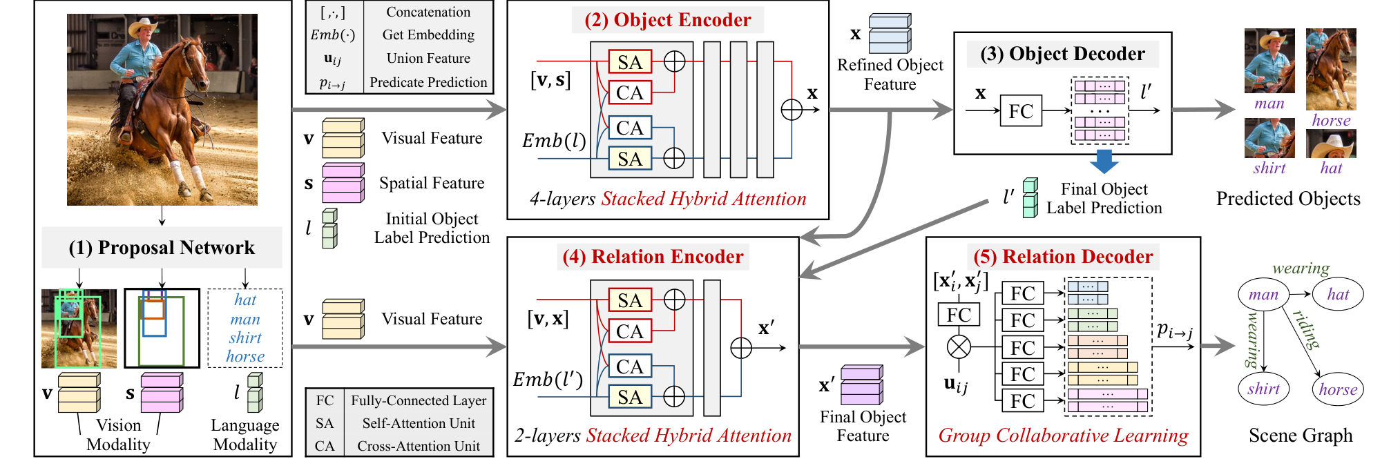
As illustrated in Figure 2, our framework is based on the common pipeline followed by typical SGG approacheszellers2018neural; tang2019learning; yan2020pcpl; yu2020cogtree, which is a regular encoder-decoder structure.
Proposal Network is actually a pre-trained object detector. Given an image , it generates a set of object predictions . For each object , it provides a visual feature , a spatial feature of the bounding box coordinates, and an initial object label prediction .
Object Encoder aims to obtain the refined object feature for further predictions, which is calculated as:
| (1) |
where represents the object encoder, which can be any feature refinement modules (e.g., BiLSTMs zellers2018neural and GNNschen2019knowledge), denotes the concatenation operation, represents a fully-connected layer, and refers to a pre-trained language model to acquire the semantic feature of based on its initial object label prediction .
Object Decoder aims to obtain the final object label prediction based on the refined object feature , which is calculated as:
| (2) |
where represents the object decoder, which is a single fully-connected layer.
Relation Encoder works on obtaining the final object feature for predicate predictions, which is calculated as:
| (3) |
where represents the relation encoder, which shares the same architecture with the object encoder.
Relation Decoder is responsible for predicting the predicate label based on the final object features of subject and object , which is calculated as:
| (4) |
where represents the relation decoder. We also follow zellers2018neural to employ the union feature of the object pair (, ) to enhance the predicate predictions.
It is worth noting that we improve three key components marked in red in Figure 2 to promote the unbiased SGG. Specifically, for the object encoder and the relation encoder, we propose the Stacked Hybrid-Attention (SHA) network to alleviate the insufficient modality fusion problem. Regarding the relation decoder, we devise the Group Collaborative Learning (GCL) strategy to address the intractable biased relationship prediction problem.

3.3 Encoder: Stacked Hybrid-Attention
Beyond understanding the visual contents (object proposals) of a given image, the semantic cues (refer to the class names in SGG) are also indispensable for robust relationship predictions. Unfortunately, most of the approaches in SGG simply fuse these two modal features by summing up directly or concatenation, which may be insufficient to mine the underlying inter-modal interaction, thus resulting in sub-optimal performance. To address this deficiency, we propose the Stacked Hybrid Attention (SHA) network, which is composed of several SHA layers. Each SHA layer contains two parallel Hybrid-Attention (HA) cells, and each HA cell is a composition of two types of attention units, i.e., the Self-Attention (SA) unit to facilitate the intra-modal refinement, and the Cross-Attention (CA) unit to model the inter-modal interaction. As shown in Figure 3, both the SA unit and CA unit are built upon a multi-head attention module and a feed-forward module based on the attention mechanismvaswani2017attention. The difference between SA and CA is whether the input features belong to the same modality.
Ultimately, we build our SHA network by cascading SHA layers in sequential order. For the -th SHA layer, the feature propagation process can be formulated as:
| (5) |
where and denote the self-attention and cross-attention computation, respectively. For the first SHA layer, we set its input feature and , where and denote the original visual feature and semantic feature, respectively. After obtaining the final visual feature and semantic feature generated by the last SHA layer, we sum them up to get the refined output, which contains rich multi-modal interaction information.
3.4 Decoder: Group Collaborative Learning
As aforementioned, when facing an extremely unbalanced dataset, a naive SGG model could hardly achieve a satisfactory prediction performance on all the predicate classes. Towards this end, we aim to deploy several classifiers which are expert in distinguishing different subsets of predicates, and organize these classifiers to cooperatively address the biased relationship predictions. Based on this “divide-conquer-cooperate” intention, we propose the Group Collaborative Learning (GCL) strategy. As shown in Figure 4, GCL contains five key steps as follows:
Predicate Class Grouping aims to split the unbalanced dataset into several relatively balanced groups, and then configure the classification space for all the classifiers. Based on the observation that the recognition capability would suffer from the biased data distribution, we aim to provide each classifier with a relatively balanced training set, thus it could adequately learn the discriminating representations towards a subset of predicates. Therefore, We first sort the predicate classes by their amount of training instances in descending order, obtaining a sorted set . We then divide into mutually exclusive groups according to the pre-defined threshold . The workflow is summarized in Algorithm 1, where denotes the amount of training instances towards the predicate . Line 3 in Algorithm 1 ensures that, for each group , the maximal amount of training instances will be no more than times of the minimal amount, thus the predicates in share a relatively equal amount.
We then borrow the idea from the class-incremental learning hu2020learning, and deploy a set of classifiers which follow a continuously growing classification space. Except for the first classifier , other classifiers should recognize the predicate classes from both previous and current groups, i.e., the classification space in is . Note that we only choose the last classifier to obtain the final predicate predictions in the evaluation stage.
Balanced Sample Preparation aims to achieve several balanced training sets provided for further joint optimization by re-sampling the instances. For each classifier that incorporates a newly-added group to extend the previous classification space as , we expect it could adequately learn the discriminating representations towards the predicates, particularly within the newly-added group . Therefore, for the predicates in the group , we should retain all of its training instances to facilitate the convergence. And for the predicates in the previous classification space , since they have more samples in the original dataset, we should under-sample their training instances to avoid biased predictions.
To implement this intention, we propose the Median Re-Sampling strategy to perform the re-sampling operation. For each classification space , we first calculate the median amount over all the classes within . For example, if is sorted in descending order and contains 9 predicate classes, the median amount is equal to . Then for each predicate class in , we calculate the sampling rate as follows:
| (6) |
By employing the above strategy, each classifier would be expert in distinguishing the predicates, particularly in the newly-added group. For example, since we would under-sample the instances in Group 3 for training the and classifiers, the classifier is more likely to achieve a better performance in distinguishing the predicates in Group 3, as we retain all the samples of this group to let the classifier adequately learn the discriminating representations.
Class Probability Prediction aims to parse the sampled instances into the class probability logits for further loss computation and model optimization. For an object pair chosen by the Median Re-Sampling strategy, after obtaining the subject feature , the object feature , and their union feature , the class probability prediction generated by the classifier is calculated as follows:
| (7) |
where denotes the element-wise product.
Parallel Classifier Optimization aims to regularize the final classifier by jointly optimizing all the classifiers. In the training stage, the parameters of all the predicate classifiers would be optimized simultaneously, where the objective function can be defined as:
| (8) |
where denotes the set of the object pairs chosen by the Median Re-Sampling strategy, denotes the length of the given set, denotes the ground-truth predicate label of the object pair , and is a regular Cross-Entropy cost function.
The Parallel Classifier Optimization can be seen as a “weak constraint” for Group Collaborative Learning, since we expect that gathering gradients from all the classifiers would facilitate the convergence of the final classifier .
Collaborative Knowledge Distillation aims to establish a knowledge transfer mechanism to promote the unbiased prediction capability of the final classifier . As aforementioned, each classifier specializes in distinguishing the predicates, particularly within the newly-added group. In order to preserve and translate this well-learned knowledge to compensate for the under-fitting on the head classes, we propose the Collaborative Knowledge Distillation (CKD), whose objective function is defined as:
| (9) |
where denotes the set of pairwise knowledge matching from the classifier to the classifier (). We provide two alternatives, namely Adjacent and Top-Down strategy, to configure the set (these two strategies are illustrated in Figure 6 and Parameter Analysis). Note that the output generated by the classifier incorporates new predicate classes which are not included in the previous classification space , we utilize to indicate the sliced output by cutting off the incrementally-added classes which are not included in , thus ensuring that shares the same dimension as . is a regular Kullback-Leibler Divergence loss, which is defined as:
| (10) |
By taking the previous predicate probability output from the classifier as the soft label, CKD forces the current classifier to mimic the prediction behaviour that is expert in, thus can be treated as a “strong constraint”.
Ultimately, the objective function of our proposed Group Collaborative Learning (GCL) is the combination of PCO and CKD, which is defined as:
| (11) |
where is the pre-defined hyper-parameters to weigh the total loss . By employing these two types of constraint, we effectively mitigate the overwhelming punishments to the tail classes and compensate for the under-fitting on the head ones, which benefits in establishing a reasonable trade-off during the predicate predictions.
| Model | PredCls | SGCls | SGDet | ||||||
|---|---|---|---|---|---|---|---|---|---|
| mR@20 | mR@50 | mR@100 | mR@20 | mR@50 | mR@100 | mR@20 | mR@50 | mR@100 | |
| IMP+† | - | 9.8 | 10.5 | - | 5.8 | 6.0 | - | 3.8 | 4.8 |
| KERN† | - | 17.7 | 19.2 | - | 9.4 | 10.0 | - | 6.4 | 7.3 |
| GPS-Net† | 17.4 | 21.3 | 22.8 | 10.0 | 11.8 | 12.6 | 6.9 | 8.7 | 9.8 |
| PCPL† | - | 35.2 | 37.8 | - | 18.6 | 19.6 | - | 9.5 | 11.7 |
| VTransE+ | 13.6 | 17.1 | 18.6 | 6.6 | 8.2 | 8.7 | 5.1 | 6.8 | 8.0 |
| SG-CogTree | 22.9 | 28.4 | 31.0 | 13.0 | 15.7 | 16.7 | 7.9 | 11.1 | 12.7 |
| BGNN | - | 30.4 | 32.9 | - | 14.3 | 16.5 | - | 10.7 | 12.6 |
| Motifs | 11.7 | 14.8 | 16.1 | 6.7 | 8.3 | 8.8 | 5.0 | 6.8 | 7.9 |
| Motifs + Reweightd | 14.3 | 17.3 | 18.6 | 9.5 | 11.2 | 11.7 | 6.7 | 9.2 | 10.9 |
| Motifs + TDEd | 18.5 | 25.5 | 29.1 | 9.8 | 13.1 | 14.9 | 5.8 | 8.2 | 9.8 |
| Motifs + CogTreed | 20.9 | 26.4 | 29.0 | 12.1 | 14.9 | 16.1 | 7.9 | 10.4 | 11.8 |
| Motifs + DLFEd | 22.1 | 26.9 | 28.8 | 12.8 | 15.2 | 15.9 | 8.6 | 11.7 | 13.8 |
| Motifs + EBMd | 14.2 | 18.0 | 28.8 | 8.2 | 10.2 | 11.0 | 5.7 | 7.7 | 9.3 |
| Motifs + GCL | 30.5 | 36.1 | 38.2 | 18.0 | 20.8 | 21.8 | 12.9 | 16.8 | 19.3 |
| VCTree | 13.1 | 16.7 | 18.1 | 9.6 | 11.8 | 12.5 | 5.4 | 7.4 | 8.7 |
| VCTree + Reweightd | 16.3 | 19.4 | 20.4 | 10.6 | 12.5 | 13.1 | 6.6 | 8.7 | 10.1 |
| VCTree + TDEd | 18.4 | 25.4 | 28.7 | 8.9 | 12.2 | 14.0 | 6.9 | 9.3 | 11.1 |
| VCTree + CogTreed | 22.0 | 27.6 | 29.7 | 15.4 | 18.8 | 19.9 | 7.8 | 10.4 | 12.1 |
| VCTree + DLFEd | 20.8 | 25.3 | 27.1 | 15.8 | 18.9 | 20.0 | 8.6 | 11.8 | 13.8 |
| VCTree + EBMd | 14.2 | 18.2 | 19.7 | 10.4 | 12.5 | 13.5 | 5.7 | 7.7 | 9.1 |
| VCTree + GCL | 31.4 | 37.1 | 39.1 | 19.5 | 22.5 | 23.5 | 11.9 | 15.2 | 17.5 |
| SHA | 14.4 | 18.8 | 20.5 | 8.7 | 10.9 | 11.6 | 5.7 | 7.8 | 9.1 |
| SHA + GCL (ours) | 35.6 | 41.6 | 44.0 | 19.6 | 23.0 | 24.3 | 14.2 | 17.9 | 20.9 |
| Model | PredCls | SGCls | SGDet |
|---|---|---|---|
| mR 50/100 | mR 50/100 | mR 50/100 | |
| VTransE | 14.0 / 15.0 | 8.1 / 8.7 | 5.8 / 6.6 |
| VTransE + GCL | 30.4 / 32.3 | 16.6 / 17.4 | 14.7 / 16.4 |
| Motifs | 16.4 / 17.1 | 8.2 / 8.6 | 6.4 / 7.7 |
| Motifs + GCL | 36.7 / 38.1 | 17.3 / 18.1 | 16.8 / 18.8 |
| VCTree | 16.6 / 17.4 | 7.9 / 8.3 | 6.5 / 7.4 |
| VCTree + GCL | 35.4 / 36.7 | 17.3 / 18.0 | 15.6 / 17.8 |
| SHA | 19.5 / 21.1 | 8.5 / 9.0 | 6.6 / 7.8 |
| SHA + GCL | 41.0 / 42.7 | 20.6 / 21.3 | 17.8 / 20.1 |
4 Experiments
4.1 Experimental Settings
Dataset. We present the experimental results on two datasets: Visual Genome (VG) krishna2016visual and GQA hudson2019gqa. VG is the most widely-used benchmark for SGG, which is composed of more than 108K images and 2.3M relation instances. Following the prior approaches xu2017scene; chen2019knowledge; lin2020gps; yan2020pcpl; zhang2017visual; li2021bipartite; zellers2018neural; tang2019learning; tang2020unbiased; yu2020cogtree; chiou2021recovering; suhail2021energy, we adopt the most widely-used VG150 split, which contains the most frequent 150 object classes and 50 predicate classes. GQA is another vision-and-language benchmark with more than 3.8M relation annotations. In order to achieve a representative split like VG150, we manually clean up a substantial fraction of annotations that have poor-quality or ambiguous meanings, and then select Top-200 object classes as well as Top-100 predicate classes by their frequency, thus establishing the GQA200 split. For both VG150 and GQA200, we use 70 of the images for training and the remaining 30 for testing. We also follow zellers2018neural to sample a 5K validation set from the training set for parameter tuning.
Tasks. To comprehensively evaluate the performance, we follow three conventional tasks: 1) Predicate Classification (PredCls) predicts the relationships of all the pairwise objects by employing the given ground-truth bounding boxes and classes; 2) Scene Graph Classification (SGCls) predicts the objects classes and their pairwise relationships by employing the given ground-truth object bounding boxes; and 3) Scene Graph Detection (SGDet) detects all the objects in an image, and predicts their bounding boxes, classes and pairwise relationships.
Evaluation Metrics. Following yan2020pcpl; lin2020gps; li2021bipartite; tang2020unbiased; yu2020cogtree; chiou2021recovering; suhail2021energy, we use mean Recall@K (mR@K)tang2019learning; chen2019knowledge, which computes the average Recall@K (R@K) for each predicate class, to evaluate the unbiased SGG. As R@K is easily dominated by the head classes due to the extremely unbiased dataset, mR@K could give a fair performance appraisal for both head and tail classes, which is widely used as an unbiased evaluation metric.
Implementation Details. We adopt a pre-trained Faster R-CNN Ren2017Faster with ResNeXt-101-FPNxie2017aggregated provided by tang2020unbiased as the object detector. We employ Glovepennington2014glove to obtain the semantic embedding. The object encoder and the relation encoder contain four and two SHA layers, respectively. We set the division threshold , and employ the Top-Down strategy (each classifier is forced to learn the prediction behavior from all its predecessors, see Figure 6 for more details) to construct the pairwise knowledge matching set . The hyper-parameter which balances the optimization objective is set to be 1.0. We optimize the proposed network by the Adam optimizer with a momentum of 0.9. For all three tasks, the total training stage lasts for 60,000 steps with a batch size of 8. The initial learning rate is 0.001, and we adopt the same warm-up and decayed strategy as tang2020unbiased. One RTX2080 Ti is used to conduct all the experiments.
4.2 Compared Methods
We want to declare that our proposed method is not only powerful in generating unbiased scene graphs, but also applicable for a variety of SGG approaches. For the former, we compare it with state-of-the-art approaches, including re-produced IMP+xu2017scene, KERNchen2019knowledge, GPS-Netlin2020gps, PCPLyan2020pcpl, re-produced VTransE+zhang2017visual and BGNNli2021bipartite. For the latter, we adopt two typical baselines, namely Motifszellers2018neural and VCTreetang2019learning, to give a fair comparison with other model-agnostic approaches, such as Reweightingchiou2021recovering, TDEtang2020unbiased, CogTreeyu2020cogtree, DLFEchiou2021recovering and EBMsuhail2021energy.
Table 1 and Table 2 present the performance of different approaches conducted on VG150 and GQA200, respectively. We have several observations as follows: 1) Our proposed SHA+GCL significantly outperforms all the baselines on all three tasks. To the best of our knowledge, our work is the first to breakthrough the 40% precision in both mR@50 and mR@100 on PredCls, and we also achieve the best performance on SGCls and SGDet. 2) Motifs+GCL and VCTree+GCL nearly double the performance in mean Recall on all three tasks compared with Motifs and VCTree. It demonstrates that the proposed GCL is model-agnostic and can largely enhance the unbiased relationship predictions. 3) Compared with Motifs+GCL and VCTree+GCL, we witness an obvious performance gain in SHA+GCL. It indicates that the proposed SHA module could facilitate both the intra-modal refinement and the inter-modal interaction, thus leading to more accurate predictions. In conclusion, SHA+GCL effectively addresses two aforementioned concerns in SGG, i.e., insufficient modality fusion and biased relationship predictions.
4.3 Ablation Study
As aforementioned, we propose the Stacked Hybrid Attention (SHA) network to improve the object encoder and the relation encoder, and propose the Group Collaborative Learning (GCL) strategy, which employs the Parallel Classifier Optimization (PCO) as the “weak constraint” and Collaborative Knowledge Distillation (CKD) as the “strong constraint”, to guide the training of the decoder. In order to prove the effectiveness of the above components, we test various ablation models on VG150 as follows:
- •
w/o-GCL: To evaluate the effectiveness of GCL, we let the relation decoder be a one-layer classifier, where a regular Cross-Entropy loss is performed.
- •
w/o PCO&CKD: To evaluate the effectiveness of PCO in GCL, we remove the PCO loss and CKD loss, and only employ the Median Re-Sampling strategy and a regular Cross-Entropy loss in the optimization step.
- •
w/o CKD: To evaluate the effectiveness of CKD in GCL, we remove the CKD loss but retain all the classifiers to compute the PCO loss.
- •
w/o CA or w/o SA: To evaluate the effectiveness of SHA, we remove either the Cross-Attention (CA) unit or the Self-Attention (SA) unit in every SHA layer.
| Model | PredCls | SGCls | SGDet |
|---|---|---|---|
| mR 50/100 | mR 50/100 | mR 50/100 | |
| w/o - GCL | 18.8 / 20.5 | 10.9 / 11.6 | 7.8 / 9.1 |
| w/o - PCO&CKD | 35.2 / 37.4 | 20.1 / 21.2 | 14.6 / 16.9 |
| w/o - CKD | 39.3 / 41.7 | 22.0 / 23.2 | 16.5 / 19.0 |
| w/o - CA | 39.8 / 42.5 | 22.6 / 23.6 | 16.8 / 19.3 |
| w/o - SA | 39.2 / 41.5 | 22.6 / 23.7 | 17.5 / 20.1 |
| SHA + GCL | 41.6 / 44.0 | 23.0 / 24.3 | 17.9 / 20.9 |
Table 3 presents the results of all the ablation models. We have several observations as follows: 1) Compared with w/o-GCL, SHA+GCL nearly doubles the performance. Moreover, in Figure 5(a), we compare w/o-GCL and SHA+GCL with respect to R@100 of all the predicate classes. As can be observed, SHA+GCL obviously improves the performance on most of the predicate classes, only with an acceptable decay on the head classes in Group 1 and Group 2, showing a powerful capability in generating unbiased scene graphs. 2) Compared with w/o-PCO&CKD, w/o-CKD evidently improves the prediction performance, demonstrating that the “weak constraint”, namely gathering gradients from all the classifiers, would facilitate the convergence of the final classifier. 3) Compared with w/o-CKD, we witness an obvious performance gain in SHA+GCL. Moreover, we compare w/o-CKD and SHA+GCL on the detailed precision towards every predicate class on VG150. As shown in Figure 5(b), CKD effectively prevents the model from sacrificing much on the head classes, as well as achieves a comparable performance towards the tail predictions. It demonstrates that the “strong constraint”, namely a knowledge transfer paradigm, could effectively compensate for the under-fitting on the head classes by preserving the discriminating capability learned previously, and thus benefits in achieving a reasonable trade-off. 4) From the last three rows in Table 3, we witness an obvious performance decay when removing either the CA unit or the SA unit. It verifies that combining both attentions would effectively alleviate the insufficient modality fusion, thus leading to more accurate predictions.
4.4 Parameter Analysis
As aforementioned, the threshold and the organization strategy would influence the performance of GCL. As Figure 6 illustrates, for the former, we set 3, 4, and 5, and obtain 6, 5, and 4 group divisions, respectively. For the latter, we provide two alternatives, namely Adjacent and Top-Down strategy, whose difference is whether each classifier could learn the knowledge from its nearest predecessor (Adjacent) or from all the predecessors (Top-Down).
| Model | PredCls | SGCls | SGDet | |
|---|---|---|---|---|
| Strategy | mR 50/100 | mR 50/100 | mR 50/100 | |
| 3 | Adjacent | 40.0 / 42.4 | 22.5 / 23.4 | 16.8 / 19.2 |
| 4 | Adjacent | 41.0 / 43.5 | 23.0 / 23.9 | 17.3 / 19.7 |
| 5 | Adjacent | 39.4 / 41.7 | 21.8 / 23.0 | 16.7 / 19.1 |
| 3 | Top-down | 40.9 / 43.2 | 22.9 / 23.8 | 17.0 / 19.9 |
| 4 | Top-down | 41.6 / 44.0 | 23.0 / 24.3 | 17.9 / 20.9 |
| 5 | Top-down | 39.7 / 42.0 | 23.1 / 23.8 | 16.9 / 19.6 |
Table 4 presents the performance comparisons, where and the Top-Down strategy is the best combination.
5 Conclusion
In this work, we declare two concerns that restrict the practical applications of SGG, namely insufficient modality fusion and biased relationship predictions. To address such deficiency, we propose the Stacked Hybrid-Attention network and the Group Collaborative Learning strategy. In this way, we establish a new state-of-the-art in the unbiased metric and provide a model-agnostic debiasing method. In the future, we plan to explore more robust group dividing methods and devise more knowledge distillation strategies.
Acknowledgments. This work is supported by the National Natural Science Foundation of China, No.: 62176137, No.:U1936203, and No.: 62006140; the Shandong Provincial Natural Science and Foundation, No.: ZR2020QF106; Beijing Academy of Artificial Intelligence(BAAI); Ant Group.
References
- (1) Haoli Bai, Jiaxiang Wu, Irwin King, and Michael Lyu. Few shot network compression via cross distillation. In Proceedings of the AAAI Conference on Artificial Intelligence, volume 34, pages 3203–3210, 2020.
- (2) Shizhe Chen, Qin Jin, Peng Wang, and Qi Wu. Say as you wish: Fine-grained control of image caption generation with abstract scene graphs. In Proceedings of the IEEE/CVF Conference on Computer Vision and Pattern Recognition, pages 9962–9971, 2020.
- (3) Tianshui Chen, Weihao Yu, Riquan Chen, and Liang Lin. Knowledge-embedded routing network for scene graph generation. In Proceedings of the IEEE/CVF Conference on Computer Vision and Pattern Recognition, pages 6163–6171, 2019.
- (4) Meng-Jiun Chiou, Henghui Ding, Hanshu Yan, Changhu Wang, Roger Zimmermann, and Jiashi Feng. Recovering the unbiased scene graphs from the biased ones. arXiv preprint arXiv:2107.02112, 2021.
- (5) Bo Dai, Yuqi Zhang, and Dahua Lin. Detecting visual relationships with deep relational networks. In Proceedings of the IEEE/CVF Conference on Computer Vision and Pattern Recognition, pages 3076–3086, 2017.
- (6) Helisa Dhamo, Azade Farshad, Iro Laina, Nassir Navab, Gregory D Hager, Federico Tombari, and Christian Rupprecht. Semantic image manipulation using scene graphs. In Proceedings of the IEEE/CVF Conference on Computer Vision and Pattern Recognition, pages 5213–5222, 2020.
- (7) Lingyun Feng, Minghui Qiu, Yaliang Li, Hai-Tao Zheng, and Ying Shen. Learning to augment for data-scarce domain bert knowledge distillation. arXiv preprint arXiv:2101.08106, 2021.
- (8) Mitchell A Gordon and Kevin Duh. Explaining sequence-level knowledge distillation as data-augmentation for neural machine translation. arXiv preprint arXiv:1912.03334, 2019.
- (9) Jianping Gou, Baosheng Yu, Stephen J Maybank, and Dacheng Tao. Knowledge distillation: A survey. International Journal of Computer Vision, 129(6):1789–1819, 2021.
- (10) Jiuxiang Gu, Shafiq Joty, Jianfei Cai, Handong Zhao, Xu Yang, and Gang Wang. Unpaired image captioning via scene graph alignments. In Proceedings of the IEEE/CVF International Conference on Computer Vision, pages 10323–10332, 2019.
- (11) Yutian Guo, Jingjing Chen, Hao Zhang, and Yu-Gang Jiang. Visual relations augmented cross-modal retrieval. In Proceedings of the 2020 International Conference on Multimedia Retrieval, pages 9–15, 2020.
- (12) Marcel Hildebrandt, Hang Li, Rajat Koner, Volker Tresp, and Stephan Günnemann. Scene graph reasoning for visual question answering. arXiv preprint arXiv:2007.01072, 2020.
- (13) Geoffrey Hinton, Oriol Vinyals, and Jeff Dean. Distilling the knowledge in a neural network. arXiv preprint arXiv:1503.02531, 2015.
- (14) Xinting Hu, Yi Jiang, Kaihua Tang, Jingyuan Chen, Chunyan Miao, and Hanwang Zhang. Learning to segment the tail. In Proceedings of the IEEE/CVF Conference on Computer Vision and Pattern Recognition, pages 14045–14054, 2020.
- (15) Drew A Hudson and Christopher D Manning. Gqa: A new dataset for real-world visual reasoning and compositional question answering. In Proceedings of the IEEE/CVF Conference on Computer Vision and Pattern Recognition, pages 6700–6709, 2019.
- (16) Ranjay Krishna, Yuke Zhu, Oliver Groth, Justin Johnson, Kenji Hata, Joshua Kravitz, Stephanie Chen, Yannis Kalantidis, Li-Jia Li, David A Shamma, et al. Visual genome: Connecting language and vision using crowdsourced dense image annotations. arXiv preprint arXiv:1602.07332, 2016.
- (17) Rongjie Li, Songyang Zhang, Bo Wan, and Xuming He. Bipartite graph network with adaptive message passing for unbiased scene graph generation. In Proceedings of the IEEE/CVF Conference on Computer Vision and Pattern Recognition, pages 11109–11119, 2021.
- (18) Kongming Liang, Yuhong Guo, Hong Chang, and Xilin Chen. Visual relationship detection with deep structural ranking. In Proceedings of the AAAI Conference on Artificial Intelligence, volume 32, 2018.
- (19) Wentong Liao, Bodo Rosenhahn, Ling Shuai, and Michael Ying Yang. Natural language guided visual relationship detection. In Proceedings of the IEEE/CVF Conference on Computer Vision and Pattern Recognition Workshops, pages 444–453, 2019.
- (20) Xin Lin, Changxing Ding, Jinquan Zeng, and Dacheng Tao. Gps-net: Graph property sensing network for scene graph generation. In Proceedings of the IEEE/CVF Conference on Computer Vision and Pattern Recognition, pages 3746–3753, 2020.
- (21) Cewu Lu, Ranjay Krishna, Michael Bernstein, and Li Fei-Fei. Visual relationship detection with language priors. In Proceedings of the European Conference on Computer Vision, pages 852–869, 2016.
- (22) Jiasen Lu, Dhruv Batra, Devi Parikh, and Stefan Lee. Vilbert: Pretraining task-agnostic visiolinguistic representations for vision-and-language tasks. arXiv preprint arXiv:1908.02265, 2019.
- (23) Seyed Iman Mirzadeh, Mehrdad Farajtabar, Ang Li, Nir Levine, Akihiro Matsukawa, and Hassan Ghasemzadeh. Improved knowledge distillation via teacher assistant. In Proceedings of the AAAI Conference on Artificial Intelligence, volume 34, pages 5191–5198, 2020.
- (24) Jeffrey Pennington, Richard Socher, and Christopher D Manning. Glove: Global vectors for word representation. In Proceedings of the Conference on Empirical Methods in Natural Language Processing, pages 1532–1543, 2014.
- (25) Shaoqing Ren, Kaiming He, Ross Girshick, and Jian Sun. Faster r-cnn: Towards real-time object detection with region proposal networks. IEEE Transactions on Pattern Analysis & Machine Intelligence, 39(6):1137–1149, 2017.
- (26) Sahand Sharifzadeh, Sina Moayed Baharlou, and Volker Tresp. Classification by attention: Scene graph classification with prior knowledge. arXiv preprint arXiv:2011.10084, 2020.
- (27) Zhiqiang Shen, Zechun Liu, Dejia Xu, Zitian Chen, Kwang-Ting Cheng, and Marios Savvides. Is label smoothing truly incompatible with knowledge distillation: An empirical study. arXiv preprint arXiv:2104.00676, 2021.
- (28) Xue Song, Jingjing Chen, Zuxuan Wu, and Yu-Gang Jiang. Spatial-temporal graphs for cross-modal text2video retrieval. IEEE Transactions on Multimedia, 2021.
- (29) Mohammed Suhail, Abhay Mittal, Behjat Siddiquie, Chris Broaddus, Jayan Eledath, Gerard Medioni, and Leonid Sigal. Energy-based learning for scene graph generation. In Proceedings of the IEEE/CVF Conference on Computer Vision and Pattern Recognition, pages 13936–13945, 2021.
- (30) Kaihua Tang, Yulei Niu, Jianqiang Huang, Jiaxin Shi, and Hanwang Zhang. Unbiased scene graph generation from biased training. In Proceedings of the IEEE/CVF Conference on Computer Vision and Pattern Recognition, pages 3716–3725, 2020.
- (31) Kaihua Tang, Hanwang Zhang, Baoyuan Wu, Wenhan Luo, and Wei Liu. Learning to compose dynamic tree structures for visual contexts. In Proceedings of the IEEE/CVF Conference on Computer Vision and Pattern Recognition, pages 6619–6628, 2019.
- (32) Damien Teney, Lingqiao Liu, and Anton van Den Hengel. Graph-structured representations for visual question answering. In Proceedings of the IEEE/CVF Conference on Computer Vision and Pattern Recognition, pages 1–9, 2017.
- (33) Ashish Vaswani, Noam Shazeer, Niki Parmar, Jakob Uszkoreit, Llion Jones, Aidan N Gomez, Lukasz Kaiser, and Illia Polosukhin. Attention is all you need. arXiv preprint arXiv:1706.03762, 2017.
- (34) Ji Wang, Weidong Bao, Lichao Sun, Xiaomin Zhu, Bokai Cao, and S Yu Philip. Private model compression via knowledge distillation. In Proceedings of the AAAI Conference on Artificial Intelligence, volume 33, pages 1190–1197, 2019.
- (35) Yinwei Wei, Xiang Wang, Weili Guan, Liqiang Nie, Zhouchen Lin, and Baoquan Chen. Neural multimodal cooperative learning toward micro-video understanding. IEEE Transactions on Image Processing, 29:1–14, 2019.
- (36) Yinwei Wei, Xiang Wang, Liqiang Nie, Xiangnan He, Richang Hong, and Tat-Seng Chua. Mmgcn: Multi-modal graph convolution network for personalized recommendation of micro-video. In Proceedings of the 27th ACM International Conference on Multimedia, pages 1437–1445, 2019.
- (37) Bin Wen, Jie Luo, Xianglong Liu, and Lei Huang. Unbiased scene graph generation via rich and fair semantic extraction. arXiv preprint arXiv:2002.00176, 2020.
- (38) Olivia Wiles, Sebastien Ehrhardt, and Andrew Zisserman. Co-attention for conditioned image matching. In Proceedings of the IEEE/CVF Conference on Computer Vision and Pattern Recognition, pages 15920–15929, 2021.
- (39) Saining Xie, Ross Girshick, Piotr Dollár, Zhuowen Tu, and Kaiming He. Aggregated residual transformations for deep neural networks. In Proceedings of the IEEE/CVF Conference on Computer Vision and Pattern Recognition, pages 1492–1500, 2017.
- (40) Danfei Xu, Yuke Zhu, Christopher B Choy, and Li Fei-Fei. Scene graph generation by iterative message passing. In Proceedings of the IEEE/CVF Conference on Computer Vision and Pattern Recognition, pages 5410–5419, 2017.
- (41) Pengfei Xu, Xiaojun Chang, Ling Guo, Po-Yao Huang, Xiaojiang Chen, and Alexander G Hauptmann. A survey of scene graph: Generation and application. IEEE Trans. Neural Netw. Learn. Syst, 2020.
- (42) Shaotian Yan, Chen Shen, Zhongming Jin, Jianqiang Huang, Rongxin Jiang, Yaowu Chen, and Xian-Sheng Hua. Pcpl: Predicate-correlation perception learning for unbiased scene graph generation. In Proceedings of the 28th ACM International Conference on Multimedia, pages 265–273, 2020.
- (43) Jing Yu, Yuan Chai, Yue Hu, and Qi Wu. Cogtree: Cognition tree loss for unbiased scene graph generation. arXiv preprint arXiv:2009.07526, 2020.
- (44) Zhou Yu, Jun Yu, Yuhao Cui, Dacheng Tao, and Qi Tian. Deep modular co-attention networks for visual question answering. In Proceedings of the IEEE/CVF Conference on Computer Vision and Pattern Recognition, pages 6281–6290, 2019.
- (45) Li Yuan, Francis EH Tay, Guilin Li, Tao Wang, and Jiashi Feng. Revisiting knowledge distillation via label smoothing regularization. In Proceedings of the IEEE/CVF Conference on Computer Vision and Pattern Recognition, pages 3903–3911, 2020.
- (46) Alireza Zareian, Svebor Karaman, and Shih-Fu Chang. Bridging knowledge graphs to generate scene graphs. In Proceedings of the European Conference on Computer Vision, pages 606–623, 2020.
- (47) Rowan Zellers, Mark Yatskar, Sam Thomson, and Yejin Choi. Neural motifs: Scene graph parsing with global context. In Proceedings of the IEEE Conference on Computer Vision and Pattern Recognition, pages 5831–5840, 2018.
- (48) Cheng Zhang, Wei-Lun Chao, and Dong Xuan. An empirical study on leveraging scene graphs for visual question answering. arXiv preprint arXiv:1907.12133, 2019.
- (49) Hanwang Zhang, Zawlin Kyaw, Shih-Fu Chang, and Tat-Seng Chua. Visual translation embedding network for visual relation detection. In Proceedings of the IEEE/CVF Conference on Computer Vision and Pattern Recognition, pages 5532–5540, 2017.
- (50) Lecheng Zheng, Yu Cheng, Hongxia Yang, Nan Cao, and Jingrui He. Deep co-attention network for multi-view subspace learning. In Proceedings of the Web Conference 2021, pages 1528–1539, 2021.
- (51) Yiwu Zhong, Liwei Wang, Jianshu Chen, Dong Yu, and Yin Li. Comprehensive image captioning via scene graph decomposition. In Proceedings of the European Conference on Computer Vision, pages 211–229, 2020.
1 Introduction
In this supplementary material, we present more analyses, experiments, and visualization results, as well as discuss the limitations and future work of our method.
2 Parameter Statistics
We compare the total number of parameters between three baseline methods (i.e., Motifs, VCTree, and SHA) and their enhanced versions that are equipped with our model-agnostic GCL in Table 5. As can be observed, compared with the original methods which possess a massive number of total trainable parameters (about 200M), GCL only additionally introduces a limited number of parameters (about 2M), which could hardly influence the overall training procedure.
3 Detailed Performance
We present the complete results of our experiments employing the regular Recall@Klu2016visual, the unbiased Mean Recall@Ktang2019learning; chen2019knowledge, and their meanlin2020gps on all three tasks (i.e., PredCls, SGCls, and SGDet) on VG150krishna2016visual and GQA200hudson2019gqa dataset in Table 6, where . Note that all the methods are implemented with a pre-trained Faster R-CNNRen2017Faster with ResNeXt-101-FPNxie2017aggregated provided by tang2020unbiased as the object detector, thus we could give a fair comparison to prove the superiority of our method.
From Table 6, we observe that 1) our proposed SHA+GCL achieves the best performance on all three tasks towards the unbiased metric mR@K in both two datasets. In VG150, we breakthrough the 40% precision in both mR@50 and mR@100 on PredCls, and 20% precision in mR@100 on both SGCls and SGDet, thus establishing a new state-of-the-art in the unbiased metric. 2) Our improvement towards the relation decoder, namely GCL strategy, is model-agnostic and could largely enhance the unbiased SGG. In both VG150 or GQA200, the method equipped with GCL nearly doubles the performance compared with the original one, showing the outstanding capability in generating unbiased scene graphs.
4 Visualization Results
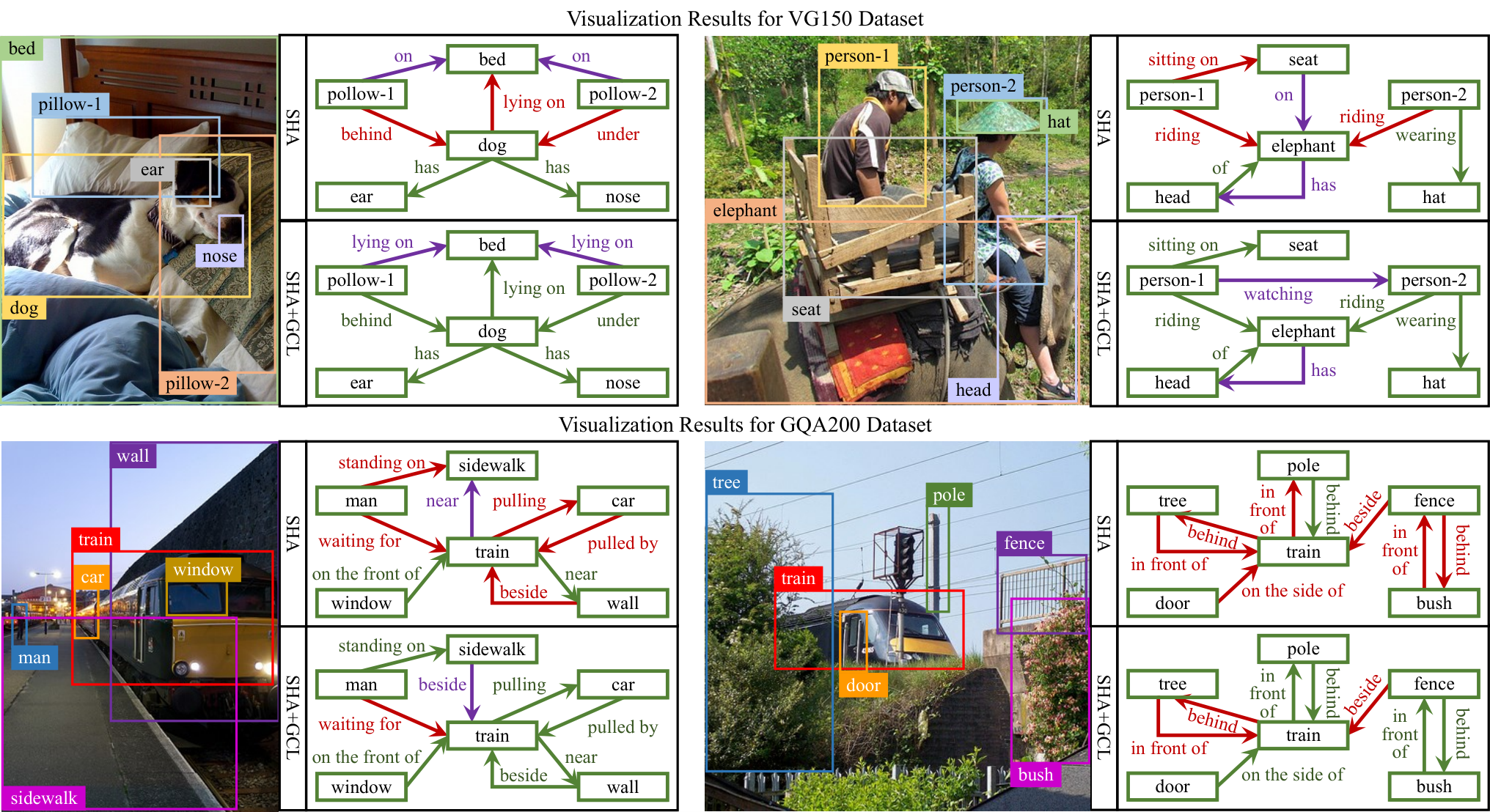
To get an intuitive perception of the superior performance in generating unbiased scene graphs of our proposed GCL, we visualize several PredCls examples generated from the biased SHA and the unbiased SHA+GCL. As shown in Figure 8, the model employing the proposed GCL strategy prefers to providing more informative and specific relationship predictions (e.g., lying on and riding) rather than common and trivial ones (e.g., on and has), e.g., “person1-riding-elephant” in the top-right example and “train-pulling-car” in the bottom-left example. Moreover, the model equipped with our model-agnostic GCL could also capture potential reasonable relationships, such as “person1-watching-person2” in the top-right example and “sidewalk-beside-train” in the bottom-left example. In a nutshell, the proposed GCL could enhance the unbiased relationship predictions, thus achieving more informative scene graphs to support various down-stream tasks.
5 Limitations and Future Work
In this section, we would like to discuss the limitations of our method, based on which we provide several potential directions to further improve our SHA+GCL.
5.1 More Configurations Could be Further Explored
As aforementioned, we follow the intuition of “divide-conquer-cooperate” to address the biased relationship predictions. In the second step, namely “conquer”, we borrow the idea from class-incremental learning hu2020learning and employ the group-incremental configuration. Actually, we employ this configuration mainly due to its simplicity and efficiency, as we could directly leverage the final classifier that covers all the candidate classes to obtain the predictions in the evaluation stage. However, we should argue that it is not the only alternative to fulfill the “conquer” step. Therefore, in the future, we aim to explore more robust group dividing methods as well as classifier configuration strategies to promote the unbiased SGG, e.g., the group-split configuration in Figure 7.
5.2 “Strong Constraint” Could be Further Enhanced
As aforementioned, in the “cooperate” step, we use the collaborative knowledge distillation to establish an effective knowledge transfer mechanism, where a regular Kullback-Leibler Divergence loss is employed. However, since various novel methods have been proposed in the knowledge distillation area, we could further enhance our GCL by devising more efficient strategies, thus strengthening the “Strong Constraint” and promoting the unbiased SGG.
| Model | Fixed | Trainable | Model | Fixed | Trainable | Model | Fixed | Trainable |
|---|---|---|---|---|---|---|---|---|
| Motifs | 158.7M | 208.5M | VCTree | 158.7M | 199.8M | SHA | 158.7M | 228.8M |
| Motifs + GCL | 158.7M | 210.5M | VCTree + GCL | 158.7M | 201.8M | SHA + GCL | 158.7M | 230.9M |
| Evaluation on Visual Genome Dataset | ||||||||
|---|---|---|---|---|---|---|---|---|
| Model | PredCls | SGCls | SGDet | MEAN | ||||
| R@50/100 | mR@50/100 | R@50/100 | mR@50/100 | R@50/100 | mR@50/100 | R-M | mR-M | |
| IMP† suhail2021energy | 61.1 / 63.1 | 11.0 / 11.8 | 37.4 / 38.3 | 6.4 / 6.7 | 23.6 / 28.7 | 3.3 / 4.1 | 42.0 | 7.2 |
| GPS-Net† li2021bipartite | 65.2 / 67.1 | 15.2 / 16.6 | 37.8 / 39.2 | 8.5 / 9.1 | 31.1 / 35.9 | 6.7 / 8.6 | 46.1 | 10.8 |
| SG-CogTree yu2020cogtree | 38.4 / 39.7 | 28.4 / 31.0 | 22.9 / 23.4 | 15.7 / 16.7 | 19.5 / 21.7 | 11.1 / 12.7 | 27.6 | 19.3 |
| BGNN li2021bipartite | 59.2 / 61.3 | 30.4 / 32.9 | 37.4 / 38.5 | 14.3 / 16.5 | 31.0 / 35.8 | 10.7 / 12.6 | 43.9 | 19.6 |
| VTransE tang2020unbiased | 65.7 / 67.6 | 14.7 / 15.8 | 38.6 / 39.4 | 8.2 / 8.7 | 29.7 / 34.3 | 5.0 / 6.0 | 45.9 | 9.7 |
| VTransE + TDE tang2020unbiased | 48.5 / 43.1 | 24.6 / 28.0 | 25.7 / 28.5 | 12.9 / 14.8 | 18.7 / 22.6 | 8.6 / 10.5 | 31.2 | 16.6 |
| VTransE + GCL | 35.4 / 37.3 | 34.2 / 36.3 | 25.8 / 26.9 | 20.5 / 21.2 | 14.6 / 17.1 | 13.6 / 15.5 | 26.2 | 23.5 |
| Motifs tang2020unbiased | 65.2 / 67.0 | 14.8 / 16.1 | 38.9 / 39.8 | 8.3 / 8.8 | 32.8 / 37.2 | 6.8 / 7.9 | 46.8 | 10.4 |
| Motifs + Reweight chiou2021recovering | 54.7 / 56.5 | 17.3 / 18.6 | 29.5 / 31.5 | 11.2 / 11.7 | 24.4 / 29.3 | 9.2 / 10.9 | 37.7 | 13.2 |
| Motifs + TDE tang2020unbiased | 46.2 / 51.4 | 25.5 / 29.1 | 27.7 / 29.9 | 13.1 / 14.9 | 16.9 / 20.3 | 8.2 / 9.8 | 32.1 | 16.8 |
| Motifs + PCPL† chiou2021recovering | 54.7 / 56.5 | 24.3 / 26.1 | 35.3 / 36.1 | 12.0 / 12.7 | 27.8 / 31.7 | 10.7 / 12.6 | 40.4 | 16.4 |
| Motifs + CogTree yu2020cogtree | 35.6 / 36.8 | 26.4 / 29.0 | 21.6 / 22.2 | 14.9 / 16.1 | 20.0 / 22.1 | 10.4 / 11.8 | 26.4 | 18.1 |
| Motifs + DLFE chiou2021recovering | 52.5 / 54.2 | 26.9 / 28.8 | 32.3 / 33.1 | 15.2 / 15.9 | 25.4 / 29.4 | 11.7 / 13.8 | 37.8 | 18.7 |
| Motifs + EMB suhail2021energy | 65.2 / 67.3 | 18.0 / 19.5 | 39.2 / 40.0 | 10.2 / 11.0 | 31.7 / 36.3 | 7.7 / 9.3 | 46.6 | 12.6 |
| Motifs + GCL | 42.7 / 44.4 | 36.1 / 38.2 | 26.1 / 27.1 | 20.8 / 21.8 | 18.4 / 22.0 | 16.8 / 19.3 | 30.1 | 25.5 |
| VCTree tang2020unbiased | 65.4 / 67.2 | 16.7 / 18.2 | 46.7 / 47.6 | 11.8 / 12.5 | 31.9 / 36.2 | 7.4 / 8.7 | 49.2 | 12.6 |
| VCTree + Reweight chiou2021recovering | 60.7 / 62.6 | 19.4 / 20.4 | 42.3 / 43.5 | 12.5 / 13.1 | 27.8 / 32.0 | 8.7 / 10.1 | 44.8 | 14.0 |
| VCTree + TDE tang2020unbiased | 47.2 / 51.6 | 25.4 / 28.7 | 25.4 / 27.9 | 12.2 / 14.0 | 19.4 / 23.2 | 9.3 / 11.1 | 32.5 | 16.8 |
| VCTree + PCPL† chiou2021recovering | 56.9 / 58.7 | 22.8 / 24.5 | 40.6 / 41.7 | 15.2 / 16.1 | 26.6 / 30.3 | 10.8 / 12.6 | 42.5 | 17.0 |
| VCTree + CogTree yu2020cogtree | 44.0 / 45.4 | 27.6 / 29.7 | 30.9 / 31.7 | 18.8 / 19.9 | 18.2 / 20.4 | 10.4 / 12.1 | 31.8 | 19.8 |
| VCTree + DLFE chiou2021recovering | 51.8 / 53.5 | 25.3 / 27.1 | 33.5 / 34.6 | 18.9 / 20.0 | 22.7 / 26.3 | 11.8 / 13.8 | 37.1 | 19.5 |
| VCTree + EMB suhail2021energy | 64.0 / 65.8 | 18.2 / 19.7 | 44.7 / 45.8 | 12.5 / 13.5 | 31.4 / 35.9 | 7.7 / 9.1 | 47.9 | 13.5 |
| VCTree + GCL | 40.7 / 42.7 | 37.1 / 39.1 | 27.7 / 28.7 | 22.5 / 23.5 | 17.4 / 20.7 | 15.2 / 17.5 | 29.6 | 25.8 |
| SHA | 64.3 / 66.4 | 18.8 / 20.5 | 38.0 / 39.0 | 10.9 / 11.6 | 30.6 / 34.9 | 7.8 / 9.1 | 45.5 | 13.1 |
| SHA + GCL | 35.1 / 37.2 | 41.6 / 44.1 | 22.8 / 23.9 | 23.0 / 24.3 | 14.9 / 18.2 | 17.9 / 20.9 | 25.4 | 28.6 |
| Evaluation on GQA Dataset | ||||||||
| Model | PredCls | SGCls | SGDet | MEAN | ||||
| R@50/100 | mR@50/100 | R@50/100 | mR@50/100 | R@50/100 | mR@50/100 | R-M | mR-M | |
| VTransE | 55.7 / 57.9 | 14.0 / 15.0 | 33.4 / 34.2 | 8.1 / 8.7 | 27.2 / 30.7 | 5.8 / 6.6 | 39.9 | 9.6 |
| VTransE + GCL | 35.5 / 37.4 | 30.4 / 32.3 | 22.9 / 23.6 | 16.6 / 17.4 | 15.3 / 18.0 | 14.7 / 16.4 | 25.4 | 21.4 |
| Motifs | 65.3 / 66.8 | 16.4 / 17.1 | 34.2 / 34.9 | 8.2 / 8.6 | 28.9 / 33.1 | 6.4 / 7.7 | 43.9 | 10.9 |
| Motifs + GCL | 44.5 / 46.2 | 36.7 / 38.1 | 23.2 / 24.0 | 17.3 / 18.1 | 18.5 / 21.8 | 16.8 / 18.8 | 29.7 | 24.2 |
| VCTree | 63.8 / 65.7 | 16.6 / 17.4 | 34.1 / 34.8 | 7.9 / 8.3 | 28.3 / 31.9 | 6.5 / 7.4 | 43.1 | 10.5 |
| VCTree + GCL | 44.8 / 46.6 | 35.4 / 36.7 | 23.7 / 24.5 | 17.3 / 18.0 | 17.6 / 20.7 | 15.6 / 17.8 | 29.6 | 23.6 |
| SHA | 63.3 / 65.2 | 19.5 / 21.1 | 32.7 / 33.6 | 8.5 / 9.0 | 25.5 / 29.1 | 6.6 / 7.8 | 41.6 | 12.1 |
| SHA + GCL | 42.7 / 44.5 | 41.0 / 42.7 | 21.4 / 22.2 | 20.6 / 21.3 | 14.8 / 17.9 | 17.8 / 20.1 | 27.3 | 27.3 |