Orientation Adaptive Minimal Learning Machine: Application to Thiolate-Protected Gold Nanoclusters and Gold-Thiolate RingsPreprint: AIP/123-QED
Abstract
Machine learning (ML) force fields are one of the most common applications of ML methods in the field of physical and chemical science. In the optimal case, they are able to reach accuracy close to the first principles methods with significantly lowered computational cost. However, often the training of the ML methods rely on full atomic structures alongside their potential energies, and applying the force information needs special modifications to standard algorithms. Here we apply distance-based ML methods to predict force norms and estimate the directions of the force vectors of the thiolate-protected gold nanoclusters. The method relies only on local structural information without energy evaluations. We apply the atomic ML forces on the structure optimization of the gold-thiolate rings, nanocluster and two known structural isomers of the nanocluster. The results demonstrate that the method is well-suited for the structural optimizations of the gold-thiolate systems, where the atomic bonding has a covalent nature in the ligand shell and at the metal-ligand interface. The methodology could be seen as an early attempt to introduce equivariant learning to distance-based ML methods.
Keywords:
Machine learning, distance-based, force vectors, clusters, goldI Introduction
Monolayer-protected clusters (MPCs) are chemically diverse nanostructures consisting of metallic core, protecting organic ligand layer and an interface structure between Tsukuda and Häkkinen 2015. The ligand layer stabilizes the metal particles, which would otherwise agglomerate or react with outside environment. Stabilization enables MPCs to have atomically precise structures. This chemically complex yet atomically well-defined nature of MPCs makes them an interesting research subject, where possible applications vary from catalysis and biological imaging to nanomedicine Tsukuda and Häkkinen 2015; Malola and Häkkinen 2021. Understanding the operational mechanisms of the MPCs in these applications requires development of efficient and reliable novel computational strategies.
Density functional theory (DFT) was introduced over half a century ago by Hohenberg and Kohn Hohenberg and Kohn 1964 and it has developed into the main tool in the field of computational nanoscience. However, DFT often requires lots of computational resources to be run in a reasonable amount of time. This has lead into development of various force fields, which accelerate the computations. For MPCs there have been developed, for example, ReaxFF Bae and Aikens 2013 and AMBER-GROMACS Pohjolainen et al. 2016 force fields. The drawback of these methods is that one has to compromise accuracy and often one still needs to do extensive parameter optimization. The introduction of machine learning (ML) methods to physical and chemical sciences have offered alternative approaches to atomic simulations. ML methods are not strictly bound by predefined mathematical functions imitating physical and chemical behavior but they are used to find underlying trends on given data. This has lead into numerous ML force fields, which are able to produce similar behavior of atoms as DFT in well-defined cases with fewer computational resources Noé et al. 2020; Unke et al. 2021a; Friederich et al. 2021. However, even if ML force fields are one of the most common applications of ML methods in the research field, underlying algorithms are general and their applications are not restricted on force fields. They also have many application in material informatics Schmidt et al. 2019; Schleder et al. 2019, catalysis research Toyao et al. 2020 and they can even be trained to build materials Jørgensen et al. 2019; Meldgaard et al. 2020; Christiansen et al. 2020.
MPCs form a challenging nanomaterial class for ML methods, because of their chemical complexity and general low-symmetry molecular structure. However, there have been some successful studies on the subject. For example, artificial neural networks and support vector machine have been used to study synthesis and properties of MPCs Li et al. 2019; Copp et al. 2020, a rule-based method has been utilized to compare local atomic environments and to construct metal-ligand interfaces Malola et al. 2019, and distance-based ML methods have been used to predict potential energies of nanocluster for finite temperature Monte Carlo simulations of their dynamical propertiesPihlajamäki et al. 2020. is also the focus of this study. This MPC has two known isomers: a cylindrical Q isomer Qian et al. 2010 and an oblate-like T Tian et al. 2015. The structures are visualized in FIG. 1.
The structural difference of these two isomers can be highlighted by writing their chemical formula using the "divide and protect" idea Häkkinen, Walter, and Grönbeck 2006. This means that the metallic core and protecting layer can be thought as separate entities and naturally notation should emphasize it. This way Q isomer could be written as Au23@SR-Au-SR-Au-SRSR-Au-SR and T isomer Au23@SR-Au-SR-Au-SR-Au-SRSR-Au-SR-Au-SRSR-Au-SRSR, where the superscript refers to a bridge site and R denotes the organic part of the thiolate. In this notation it is clear that both isomers have 23 gold atom core and protecting layers consisting of gold-thiolate oligomers or units of varying lengths. Both isomers have been found experimentally and Q isomer is thermodynamically more stable than T isomer as shown both by experiments and DFT calculations Tian et al. 2015; Juarez-Mosqueda, Malola, and Häkkinen 2019; Taylor and Mpourmpakis 2017. Having two distinct structural isomers makes this MPC a very appealing testing ground for ML methods, because one can use the data from both isomers to test the generalizability of the method.
In this study we present a local force-based ML approach to simulate atomic systems. There are already some ML methods that can be trained with forces only, such as GAP Bartók et al. 2010; Deringer et al. 2021, sGDML Chmiela et al. 2019, NequIP Batzner et al. 2022 and PaiNN Schütt, Unke, and Gastegger 2021. However, methods like GAP and sGDML rely on explicit derivatives applied to the kernel matrix. Derivatives can be costly to calculate, if analytic forms are not available. Sometimes calculation of the analytic derivatives is not feasible for variety of reasons. This might be because of the complexity of the mathematical expression but more often it is simply due to the practical reasons. One might be using for some part of the method a separate pre-made package, which does not have derivatives. In order to generate correct derivatives one would need to fully understand how the base method is implemented. In this case user might lack the resources to further explore technical details or the access to the source code might be limited by a commercial license.
Equivariant learning methods, such as NequIP Batzner et al. 2022 and PaiNN Schütt, Unke, and Gastegger 2021, address this in a different manner. They learn representations directly from the atomic numbers and coordinates in the spirit of SchNet framework Schütt et al. 2017a; Schütt et al. 2018; Schütt et al. 2019. Instead of just forming invariant representations, which are adequate to predict scalar values such as potential energy, they also preserve orientation information. This enables the prediction of directional output, such as force vectors and stress tensors. However, this kind of equivariant learning methods are currently relying on complex deep neural networks (NNs). Conventional kernel methods are still mostly utilizing derivatives.
Instead of training a ML method to predict potential energies for given configurations and then taking a gradient to obtain forces, we train our method to predict directly force vectors subjecting to individual atoms. According to the Hellman-Feynman theorem, if the Born-Oppenheimer approximation is valid, the forces are true quantum mechanical observables Hellman 1937; Feynman 1939. Hence, they can be solved analytically separately from the energy calculation, which justifies the approach to use ML to predict forces directly. The goal is to create a model that handles atoms locally, which gives it a great potential to be generalized over different systems with similar local features. This kind of an generalizability has shown to be achievable at least for methods predicting electron density Fabrizio et al. 2019; Grisafi et al. 2019.
Estimating force vector directly independent from the energy has some special advantages. Forces are local properties of an atomic system, therefore the developed ML method would naturally be local and have promising generalization possibilities. Many methods are designed to predict how much every atom contributes to the potential energy Bartók et al. 2010; Deringer et al. 2021; Schütt et al. 2017b; Schütt et al. 2017a; Schütt et al. 2018; Schütt et al. 2019; Chen et al. 2018; Batzner et al. 2022; Schütt, Unke, and Gastegger 2021; Unke et al. 2021b and it has become standard approach in many ML applications. However, training a model with energies is still dependent on full structures of the atomic systems, because potential energy cannot be unambiguously separated from the full structure. Hence, the ML method has to learn on its own to divide the energy into local contributions, which is not a trivial task. On contrary, the model focusing solely on forces is not constrained by the use of full atomic structures. One could freely collect data sets from various systems with similar chemical composition, which eases the data generation process. The disadvantage of this approach is that forces are not strictly energy conserving anymore, therefore one has to consider what applications are suitable for this kind of methods.
There have been attempts to predict directly force vectors from atomic data of metal nanoparticles and surfaces Botu and Ramprasad 2015; Botu et al. 2017; Pattnaik et al. 2020. However, these attempts use rotation variant representations of atomic environments instead of conventional rotation, translation and permutation invariant descriptors. This enables one to use conventional machine learning tools but introduces a new drawback: one has to somehow cover the orientation space. This is still a viable for lattice based systems with high symmetry. For low symmetry systems, this kind of an approach requires alignment of atomic environments and/or large amounts of rotated data. In order address this issue, the developed ML method would have to somehow utilize the idea of equivariance as mentioned above.
Our method uses conventional invariant descriptors and the ML method itself is made orientation adaptive. The approach enables fair comparison of chemical environments as the commonly used descriptors, such as Smooth Overlap of Atomic Positions (SOAP) Bartók, Kondor, and Csányi 2013, Atom-Centered Symmetry Functions (ACSF) Behler 2011, Many-Body Tensor Representation (MBTR) Huo and Rupp 2017 and numerous other descriptors Musil et al. 2021, are already well-known and tested. Our method breaks the force prediction task into two parts: (i) prediction of the norm of the force and (ii) estimation of the direction. Both parts utilize the so-called distance-based ML, which also enables elegant prediction of different attributes from the same similarity matrix. The similarity measure, as the name suggests, is the Euclidean distance. Our framework could be considered as a proto-equivariant method, because it uses invariant representations to predict properties and by orientation adaptivity it addresses the possible rotations of the system. It is an early attempt to implement equivariance into distance-based ML methods.
We trained and tested the method by using the data previously generated from DFT-level molecular dynamics (MD) simulations of the two structural isomers of nanocluster Juarez-Mosqueda, Malola, and Häkkinen 2019. This data has already been used to predict potential energies using distance-based ML Pihlajamäki et al. 2020, therefore this study provides a logical continuation to the previous research. We have tested extensively different parameters related to the method and applied it to the structure optimization of four different systems: gold-thiolate rings, with outstretched protecting units in its ligand shell and arbitrary configurations of the and two isomers of the . Gold-thiolate rings and are especially interesting test case as they are not explicitly included into the training data, hence they demonstrate the generalization possibilities of our ML approach. Furthermore, the existence of gold-thiolate rings in cluster synthesis has been verified experimentally Hostetler et al. 1998; Chen, Templeton, and Murray 2000; Corbierre and Lennox 2005 and they have also been studied theoretically Grönbeck, Walter, and Häkkinen 2006. The tests demonstrate the usefulness of our method for coarse optimization. It can guide optimization to the close vicinity of the local minimum, which can then be reached with finer optimization via DFT. The method allows breaking and making of chemical bonds, hence in the future it could be applied to the dynamic simulations where chemical reactions can take place.

II Computational methods
Here we go through the theoretical background of the ML approach. First the SOAP descriptor is presented briefly to explain its parameters, which are tested during the model development. Then the background of the distance-based ML methods is introduced and how they are applied to our systems at hand.
II.1 Smooth Overlap of Atomic Positions
SOAP is a local descriptor, which means that it is used to describe a local chemical environment of an atom or a single point. The basic idea is to present every atom as a 3D Gaussian function, then present these functions as a series expansion using radial basis functions and spherical harmonics and, finally, collecting coefficient from the expansion into a power spectrum Bartók, Kondor, and Csányi 2013; Himanen et al. 2020. We used the version implemented in DScribe package by Himanen et al. Himanen et al. 2020 and we follow their formalism to introduce main aspects of the SOAP.
The starting point of the SOAP is to represent every atom with a three dimensional Gaussian function. Every element is handled separately and the environment of the point is written as
| (1) |
Here is an atomic number and the summation goes over all atoms of that type. The positions of these atoms are denoted with . The elegant idea behind SOAP is to use radial basis functions and spherical harmonics to form a series expansion of the form
| (2) |
The coefficients are the heart of the whole description. They are solved via integration
| (3) |
and then collected into a power spectrum
| (4) |
The values are stored into a vector, which works as a local description of the point . The equation (4) is slightly different than the one in the original publication of Bartók et al. Bartók, Kondor, and Csányi 2013. In the DScribe package Himanen et al. use real (tesseral) spherical harmonics instead of complex ones and, in addition to this, they replace polynomial radial basis functions with Gaussian type orbitals
| (5) |
This simplifies the theory and makes programming the descriptor efficient. In practise, the summation in the series does not include all indices and but they are restricted to maximum values and , which are parameters of the descriptor. The index restricts the values integer , because same way as side quantum number restrict magnetic quantum numbers. Furthermore, only atoms within some pre-defined cut-off radius , which also is a parameter, are included in to the summation in 1. For further details, see references Bartók, Kondor, and Csányi 2013; Himanen et al. 2020. In this study, we tested the effects of four SOAP parameters: , , and Gaussian broadening .
II.2 Distance-based ML tools
The basic construct in the distance-based machine learning is to use Euclidean distances between reference and input data as a measure of similarity and to predict an output using these distances. There are two main distance-based ML methods: Minimal Learning Machine (MLM) de Souza Júnior et al. 2015 and Extreme Minimal Learning Machine (EMLM) Kärkkäinen 2019. Both of them are general ML tools and they have been used successfully to predict potential energies for nanoclusters Pihlajamäki et al. 2020. Distance-based methods are especially appealing methods to study complex nanostructures, because they have been shown to work well with high-dimensional data and even out-perform deep neural networks in some cases Linja et al. 2020. This is due to the distance matrix, which effectively hides the dimensionality of the data. The same feature also makes distance-based ML methods resistant to overfitting Hämäläinen et al. 2020. In addition to this, distance-based ML methods usually have only one hyperparameter: the number of reference points, which reduces parameter testing. When applying ML methods to nanosystems, there are often several parameters to tune, such as the ones of the descriptors. This means that the user have to optimize the way how the data is presented prior the actual model can be trained. The lack of hyperparameters reduces the need for complex model fitting with different parametrizations of the descriptor.
Recently, a variation of MLM, which specifically addresses the directions of the atomic forces, was proposed: Orientation Adaptive Minimal Learning Machine (OAMLM) Pihlajamäki et al. 2021. It takes the concept of using Euclidean distances as an input space similarity measure to perform predictions but instead of predicting corresponding distances to output space references, as MLM does de Souza Júnior et al. 2015, it predicts cosines of angles between reference vectors and a target vector. It can also produce estimates for the uncertainty of the predictions to provide interesting opportunities for different applications, where uncertainty might play a role.
We go through the theory behind the distance-based ML methods to form a basis for the discussion on OAMLM and the full force prediction framework. All of these methods start with the input data and corresponding output data . In our case, contains SOAP descriptions of the chemical environments of the atoms and information about the forces, either norms or unit vectors pointing to the directions of the force vectors. Let’s first consider the simplest method EMLM, which is used to predict the norms of the forces given in . From the input data , reference points are sampled forming a reference set . The training of EMLM is done via regularized least-squares optimization problem, which is used to find optimal weights to perform regression from Euclidean distances between points in and to predict Kärkkäinen 2019.
| (6) |
Vector contains Euclidean distances between th input data point and references. is a weight matrix, which does a linear regression from kernel space to output. Constant is used for regularization, which might be useful if one has noisy data. In our case, it is fixed to the square root of machine epsilon.
The minimum of the equation 6 can be found by writing it with full matrices and finding the zero point of the first derivative.
| (7) |
| (8) |
Matrix contains all Euclidean distances between training data and references. The equation (8) is now a simple representation of the training of EMLM and it can be easily solved numerically. To predict output for an arbitrary input, one has to calculate distances between the input and references forming and then compute matrix multiplication . This is analogous to Kernelized Ridge Regression (KRR), where one has a variety of choices for kernel functions Murphy 2012.
Next we shall go through the framework of the MLM presented by de Souza et al. de Souza Júnior et al. 2015 and proceed step by step to the direction prediction scheme of the OAMLM. The main difference between MLM and EMLM is that in addition to references in input space MLM also has references in output space. The idea is not to predict directly output for certain input but to form regression between the two distance spaces.
| (9) |
Here contains Euclidean distances between the input training data points in and reference points in . , on the other hand, consists of distances between training output data in and the output reference set . is a weight matrix that performs the linear regression and is a residual, which is assumed to be small. It is shown that the approximate solution for the weight matrix is de Souza Júnior et al. 2015
| (10) |
In order to calculate output with MLM, one first predicts distances between still unknown result and output space references using input space distances and just solved weights as . The result is found by solving multilateration problem, for which there are several methods Navidi, Jr., and Hereman 1998; Hämäläinen et al. 2020.
With these derivations at our disposal, let us proceed to the OAMLM. To remind, the input space training data contains SOAP descriptions of chemical environments, which do not include directional information. For this reason OAMLM also needs coordinates of neighboring atoms as an accompanying data. In the first row is the position of the studied atom itself followed by neighbors. For every training data point there are also their unit force vectors collected into , where for all values of . Similar to MLM, OAMLM also uses references both in input and output spaces. The reference data points used are sampled into for chemical descriptors, for coordinates of the neighboring atoms and for corresponding unit force vectors.
Atomic environments can be in any spatial orientation, therefore the directions of the forces cannot be compared directly. As a solution, the coordinates of neighboring atoms in and are used to align atomic environments. In this study we used Singular Value Decomposition (SVD) based method presented originally by Arun et al. Arun, Huang, and Blostein 1987. First the atoms, for which forces are predicted, are moved to the origin and their neighbors are translated together with them to preserve the general positioning. Then matrix is formed by calculating it as
| (11) |
Index refers to the th input and stands for the th reference. With SVD one can split this matrix as . These can be further used to get a rotation matrix , which will align points in and as well as possible, when the atoms are moved to the origin as in equation (11). It is important to notice that this alignment approach depends on the order of given neighborhood points, therefore one needs to form certain rules how the environments are aligned or go through all permutations. However, OAMLM is not restricted to the alignment approach used here. In principle, it is possible to define any alignment scheme suited for specific problems.
The rotation matrices are used to align atomic neighborhoods together, which then yields estimates of alignment accuracy as
| (12) |
or
| (13) |
The same rotation matrices are also used to rotate reference unit force vectors in to be comparable with data in . Dot products between these vectors are calculated as . This dot product is the cosine of the angle between two vectors, as we are working with unit vectors, and it is evaluated by OAMLM during the prediction phase Pihlajamäki et al. 2021. The and dot products are used to form matrices and respectively.
Now one has everything needed to train the OAMLM using the same training scheme as for MLM in equation (10). in is the same as before: Euclidean distances between datapoints in and . However, out is different. As mentioned in the reference Pihlajamäki et al. 2021, OAMLM has two weight matrices: c to predict dot products and g to predict alignment successes. To acquire those out in equation (10) is substituted with c or g correspondingly. However, in this study we do not use g, which could be used for uncertainty estimation. We use only c to predict dot products.
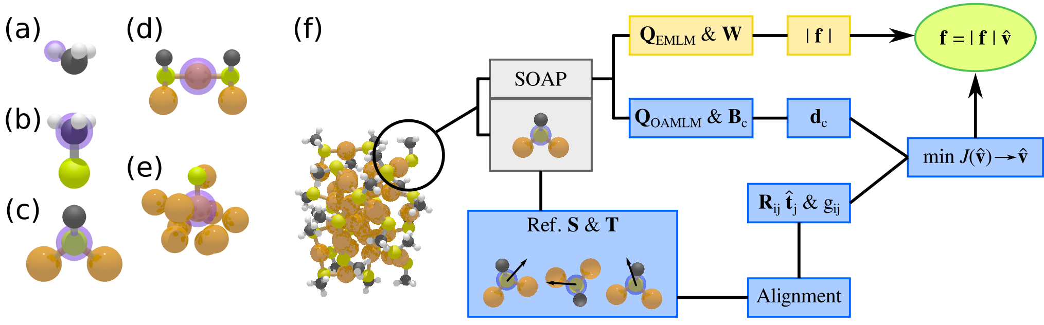
The output prediction procedure with OAMLM is similar to the methods in MLM. The schematic picture of the full force prediction process is shown in the FIG. 2. As an input, the method takes description i and its neighborhood coordinates i. Vector in is formed by calculating Euclidean distances between and the reference points in . The weight matrix is used to predict dot products as . Then reference neighborhood coordinates in are are aligned with yielding alignment accuracies and with corresponding rotation matrices reference unit vectors in are rotated accordingly. The last part of the prediction is similar to the multilateration problem. However, instead of minimizing the distance differences we minimize the difference between the predicted dot products and dot products of the rotated reference unit force vectors and yet unknown vector . There is no specific method to do this. In the reference Pihlajamäki et al. 2021 the was found numerically by using Sequential Quadratic Programming (SQP) to optimize cost function
| (14) |
We call this a numeric loss function. Here we do not make initial selection of the used reference data as in the original paper Pihlajamäki et al. 2021 but we simply use all references.
In this study we decided to also use more simple cost function as a comparison:
| (15) |
where
| (16) |
The advantage of equation (15) is that it can be solved analytically by taking a derivative over and as a result
| (17) |
The result is interestingly a weighted average of predicted projections. In practise, is not a unit vector, because there is always numeric error present in the values of c,j and , therefore one has to remember to divide it with its norm before using the result. We call equation (15) as an analytic loss function. In these two loss functions, and are parameters of the ML model and they are also tested during the model development.
II.3 Atomic force prediction scheme for
nanocluster, which is shown in FIG. 1, contains four different elements and has chemically various environments. There are covalently bound methyl thiolate ligands. There is a metallic gold core, where gold atoms are interacting with each other. On the surface of the core some gold atoms can also form bonds to the sulfur atoms. Within the metal-ligand interface structure, sulfur and gold atoms are bound with relatively covalent nature forming protecting units. Within these units the gold atoms are bound only to sulfur atoms, ideally forming two Au-S bonds. There are very diverse features determining the interactions between atoms, therefore it is a good idea to split the problem into smaller parts.
We classify the atoms into five categories: core gold atoms inside the metallic core, unit gold atoms in protecting units, sulfur, carbon and hydrogen. For every atom type we train one EMLM for force norms and one OAMLM for force directions. The norm prediction part is a straightforward standard ML problem, where the method predicts a scalar output according to a given input and the references. For the direction scheme, we have to define, which neighborhood atoms are used to align reference environments to an input environment. In principle, one could just select nearest neighbors and go through all permutations. However, this wastes computational resources by attempting many unfavorable permutations. Hence, we need to define certain rules according to physical and chemical understanding.
The most simple alignment scheme is for hydrogen. It uses only the nearest carbon, and two other nearest hydrogen atoms bound to the carbon as seen in the FIG. 2 (a). There are only two permutations of the hydrogen atoms to test. Aligning carbon is similar to the hydrogen scheme. It uses the nearest sulfur atom and three hydrogen atoms, as shown in the FIG. 2 (b), which results into six permutations of hydrogen atoms to be tested. The alignment of a sulfur atom neighborhood uses the nearest carbon and two nearest gold atoms shown in the FIG. 2 (c). There are only two permutations of the gold atoms to be tested.
The gold atoms have the most versatile chemical environments of all atoms in the cluster. Unit gold atoms use two blocks of atoms for alignment. The blocks contain the nearest sulfur atom and two other atoms bound to it: a carbon and another gold atom. Hence, there are two sulfur, two carbon and two gold atoms used to do the alignment. An example of the neighborhood structure is visualized in FIG. 2 (d). These atoms are handled as blocks, due to the linear nature of the S-Au-S bonding, therefore there are only two permutations to test.
The MD data used in model development is extremely dynamic and the nature of the Au-S bonds might change significantly. Hence, if a gold atom has only one sulfur within Å and there is no another gold atom within the same distance, the gold atom is considered to be just a half of an unit. This corresponds to a transition state where old unit is broken and new is going to be formed. In this case alignment is done by using only one block of sulfur, carbon and gold atoms. This kind of alignment is much more unstable than the standard way but fortunately breaking of S-Au bond is not a common phenomenon. For hydrogen, carbon, sulfur and unit gold atoms the alignment accuracy is calculated using the equation (12).
The environments in the metallic core gold atoms can be very homogeneous making alignment difficult. Within the core the gold atoms can be bound to a single sulfur atom and the rest of the interactions are metallic or another scenario is that all interactions are metallic. For every core gold there can be maximum of twelve neighboring atoms selected. If there is a sulfur atom within Å, it will be selected first. Then the rest are nearest gold atoms within Å from the nearest to the furthest. There can be less than twelve neighbors selected for a core gold atom, if there are not so many fulfilling the requirements as seen in the FIG. 2 (e). It is clear that there are too many neighboring atoms to go through all possible permutations in a reasonable amount of time. There can be maximum permutations for a single atomic neighborhood. In order to make the task feasible, we device two alignment schemes depending on whether the aligned gold atoms are bound to a sulfur atom or not. Alignment schemes use always the coordinates of the main gold atom itself and two neighbors, which reduces alignment time significantly. The goal is not to make perfect alignment but make as systematic as possible.
The first scenario for core gold is that both input and reference gold atoms have a sulfur atoms within their immediate vicinity. In this case, the alignment is done by using three points: gold atom itself, sulfur atom and one neighboring gold atom. For input environment we select the nearest neighboring gold atom as the third point. For reference environment the selection is the same except that in addition to the nearest neighboring gold atom we also go through all other possible neighboring gold atoms. These three atoms are used to make alignments and the accuracy is evaluated with equation (13).
The second scenario is that at least one of the environments does not contain sulfur. Here the alignment uses only three atoms similarly to the previous core gold scenario. For the input environment the three points are the atom itself and its two nearest neighbor gold atoms. For the reference environment, we use the atom itself and all possible pairs of the neighbors. Here the order does play a role, therefore one would get maximum of pairs.
These pairs together with the main gold atom form triangles, which are used to rule out some permutations. The reasoning for this ruling out is to reduce computation time. Comparing triangles is faster than making actual SVD alignments and measuring the accuracy. The difference between the th triangle of the reference environment and the triangle formed from input data is measured as
| (18) |
Here is the length of the th side of the triangle in Ångstroms and is an angle of the th corner in radians. The lower index refers to the reference data triangle and lower index to the input data triangle. Then triangles, for which the difference is the smallest, are selected. We decided to use . These triangles are used to make SVD alignments and the one yielding the smallest value of the equation (13) is selected. These two alignment schemes for core gold atoms are designed to be as similar as possible, because they will be used by the same OAMLM. If the alignment would vary much between different core gold atoms, it would make the direction estimation even more difficult for the method than it is currently.
As mentioned earlier, the number of neighborhood atoms for the core gold atoms is not constant. Hence, when the alignment success is estimated, it is required that every atom has some nearest neighbor distance. Let us clarify this via an example. If input environment has 6 neighbors and reference has 10, then after the alignment we measure the nearest neighbor distance for all 10 atoms in the reference environment and use them in the equation (13). It does not matter whether reference or input has more atoms but the accuracy is always estimated with the largest number of nearest neighbor distances. This is used to emphasize the differences between the atomic environments of the core gold atoms.
Implementing chemical rules and primary knowledge into the algorithm resembles the approach to construct metal-ligand interfaces by Malola et al. Malola et al. 2019. There authors used distances and angles to compare environments between reference structures and the environments of arbitrary points within unprotected metal clusters. This comparison enabled them to determine whether or not those points were suitable for interface atoms. Our force prediction method shows similar philosophy to the task but here we have to use actual spatial alignment in order to capture the orientation information.
II.4 Structure optimization via ML forces
As an usage example of ML forces, we perform structure optimization in different scenarios. The model does not yield values for potential energy of the system but the optimization is run solely with ML estimated forces. We used classic quasi-Newton method Broyden–Fletcher–Goldfarb–Shanno (BFGS) algorithm Broyden 1970; Fletcher 1970; Goldfarb 1970; Shanno 1970 to run structure optimization. The challenge is that ML predicted forces have always some level of uncertainty, which is seen in the optimization algorithm as a noise. In this study we do not explicitly address the uncertainty in the optimization algorithm but it is an aspect that should be considered in the future studies. The used BFGS implementation is based on the one included in Atomic Simulation Environment (ASE) package Larsen et al. 2017.
II.5 DFT methods
For reference calculations, we used the DFT code GPAW Enkovaara et al. 2010 as it was also used in the original MD simulations of by Juarez-Mosqueda et al. Juarez-Mosqueda, Malola, and Häkkinen 2019. The exchange-correlation functional was Perdew-Burke-Ernzerhof functional (PBE) Perdew, Burke, and Ernzerhof 1996 and we used real space grid spacing. BFGS structure optimization using GPAW computed potential energies and forces were run with the original implementation in ASE package Larsen et al. 2017. The DFT-level BFGS optimizations were considered to be converged if the maximum force of the atoms was .
III Results and discussion
The results are divided into six parts. First the effect of SOAP parameters to norm and direction prediction are shown. This way the optimal description parameters are found. They are used in the next two parts, where full EMLM models for norms and OAMLM models for directions are trained and tested. The last three parts focus on structure optimization. The used test cases are gold-thiolate rings, cluster structures with outstretched protecting units and snapshots from the MD simulations of the and of the both isomers of the nanocluster.
The training and testing of the models relies heavily on the DFT-level MD simulation data of the nanocluster from reference Juarez-Mosqueda, Malola, and Häkkinen 2019. In that study, authors run long MD simulations on both isomers of the , where the systems were heated from to so that they broke down. The less stable T isomer started to undergo significant structural changes very early and in the later stages highly deformed seven gold atom gold-thiolate ring broke out of the structure. These simulations resulted into over 12 000 configurations for both isomers, which serve as an ideal dataset for our study here.
III.1 Data and SOAP parameter selection
The data used to train and test our model was extracted from the DFT level MD simulations of published in the reference Juarez-Mosqueda, Malola, and Häkkinen 2019. For both isomers we sampled 1000 configurations logarithmically, which means that configurations were sampled sparsely from the beginning of the trajectory and more densely from the end in a similar fashion as log-scale graphs are plotted. This guaranteed that we got denser sampling from the high temperature region, where there are more changes in the structures, than from the low temperature region. This data contains 24 000 local environments for carbon and sulfur, 72 000 for hydrogen from both isomers. Q isomer data contains 22 836 core, 15 123 unit and 41 half unit gold atoms. T isomer data contains 22 055 core, 15 888 unit and 57 half unit gold atoms. Unit and half unit gold atoms are handled by the same EMLM and OAMLM models.
The importance of the level of description cannot be emphasized too much. If description is not accurate enough the prediction will be poor. However, if description is overly accurate, it will lead to a highly specialized model, which cannot be generalized and the risk of overfitting increases. We tested several SOAP parameters: , , and . This totals description sets for sulfur, carbon and hydrogen. For gold atoms we used only sets resulting SOAP parameter sets. In this article and its Supplemental Material, we show only a selected portion of the tests. The complete analysis of the parameter tests is available in (https://gitlab.jyu.fi/aneepihl/oamlm_forces.git).
First these sets were used to predict norms of the forces and to restrict the number of parameters to be tested in the direction prediction scheme. It is easier to predict norms than directions, therefore it is reasonable to assume that if norms are predicted inaccurately directions won’t be any better. For every parameter set we trained one EMLM with Q isomer data and one EMLM with T isomer data. Then we used Q model to predict norms from T set and vice versa. This is close to so-called cross validation approach often used when testing ML methods.
From every data set of a single isomer, 2500 points were selected with RS-maximin sampling Gonzalez 1985; Hämäläinen et al. 2020. Here data points refer to the local atomic environments and their corresponding forces. This data was used as a training data and all points were saved as references into the models. The SOAP data points were minmax scaled between 0 and 1. The performance was measured with root mean squared error (RMSE). Tests showed the most promising parameters to be , and with both and resulting to only six parameter sets to be tested with OAMLM. The results with and are shown in the Supplemental Material figures for sulfur, for carbon, for hydrogen, for unit gold and for core gold.
Testing with OAMLM was done in a similar fashion as with EMLM: models were trained with one isomer and then tested with another. As mentioned in the section II.2, the output direction estimation can be done via numeric or analytic loss function by using either equation (14) or (15). The initial tests were ran with both output estimation methods and their parameters were set as and . The performance was measured with weighted average of the angles between the estimated force directions and the corresponding DFT calculated force vectors. The squared norms of the DFT force vectors worked as weights. This emphasizes the handling of the large forces, for which it is more important to get directions correct than for the small ones. When the norm decreases the direction of the force vector becomes more and more elusive and sensitive to changes in the chemical environment.
The analytic loss function was performing better than the numeric one, which showed unstable performance. Parameters , , and showed satisfying performance for all atom types. The results with these parameters using numeric loss function are shown in Supplemental Material figure and analytic loss function results are shown in . The longer cut-off radius did not show a significant improvement compared to the selected one, therefore it is natural to use shorter one. There will be less atoms included into the description making it slightly faster to compute and it is more likely to results in generalizable method.
After finding the optimal SOAP parameters, we also tested how parameter affects the performance of the analytic loss function. In addition to the previously used value of , we also tested values and with previously acquired SOAP parameters. The results with these parameters are shown in Supplemental Material figures and . The tests do not show any significant effect to better or worse. For unit gold atoms the seem to be slightly better option than , because the weighted average angles were previously approximately and , and with smaller parameter the values decreased to about and . We settled on for unit gold atoms and for everything else .
III.2 Full EMLM force norm models
After determining suitable parameters for the SOAP description, we trained EMLM with combination of data from both Q and T isomers. From the combined data set, 5000 points for each atom type were selected with RS-maximin sampling Gonzalez 1985; Hämäläinen et al. 2020. This data was used as a training data and all points were saved as references. All descriptions were minmax scaled between 0 and 1. The models were tested with the remaining data from both isomers. The predictions are visualized in FIG. 3 along with RMSE values.
For unit gold, sulfur and hydrogen RMSEs are lower than and predictions correlate well with DFT force norms as seen in FIG. 3 (b), (c), (e), (g), (h) and (j). The largest RMSE values belong to core gold and methyl carbon model. It is expected that gold core is difficult to handle as it undergoes great deal of structural changes. Against expectations, methyl carbon proved to be difficult for the EMLM. The chemical environment of the carbon is mostly determined by its neighboring hydrogen atoms and a sulfur, therefore the changes are quite small due to the rigid covalent bonds. A logical explanation would be that the carbon needs more exact SOAP description with high sensitivity to small changes. This could be achieved by using even smaller value for Gaussian broadening parameter . However, the acquired accuracy is reasonable and can be used as a part of the simulations.

III.3 Full OAMLM force direction models
The OAMLM models were trained in same manner as EMLM but only 2500 data points were used in training and as references. The alignment of atomic environments is a relatively slow process, therefore having fewer references makes the model more feasible to use. During the predictions the weighting parameter in analytic loss function (15) was set as for unit gold atoms and for everything else . As an error measurement we used weighted average of angles between predicted force directions and DFT level force vectors. As a weights, we used the squared norms of the DFT forces the same way as before.
The results are plotted in the FIG. 4. The effects of small forces are visible in all plots. When the norm of the force is small, the direction is extremely difficult to be estimated, which leads to the increased deviation close to the zero. The weighted averages show similar trends as the RMSEs in the case of force norms. Unit gold, sulfur and hydrogen are the easiest to handle as seen in FIG. 4 (b), (c), (e), (g), (h) and (j). From these three atom types the largest the largest weighted average angle belongs to sulfur atoms of the isomer Q. The unit gold data contains some individual points, for which the angle is not as accurate as for the rest. This uncertainty is most likely caused by the inclusion of "half unit" gold atoms and possible classification difficulties. The classification rules mentioned in the section II.3 are approximate and especially the T isomer data might contain instances where classification is not clear.
For core gold atoms in the FIG. 4 (a) and (f) the points are more spread than the other atom types. This hints that the alignment of the core environment is not straightforward, which leads into difficult estimation of the direction. However, OAMLM still manages to yield reasonable estimates even with highly complex alignment situations. For the methyl carbons in the FIG. 4 (d) and (i), the origin of the uncertainty is likely the same as in the case of force norm prediction. It needs more exact SOAP description with small gaussian broadening parameter . On the other hand, it is not easy to make unambiguous alignment for the very symmetric methyl group. Hydrogen atoms do not make extreme movements, therefore all their permutations yield very similar alignments, which are difficult to distinguish without highly specialized structural descriptors.

III.4 Application to structure optimization
As we now have a full force estimation method combined from EMLMs and OAMLMs, the next step is to apply it to the structure optimization with BFGS. In the first test we leave the complicated metallic core out and focus on covalently bound parts by optimizing gold-thiolate rings. The second case is to optimize a stretched protecting unit attached to the cluster. The third one is the most difficult test, where we use our model and BFGS to optimize snapshots from the MD simulation trajectories of and .
III.4.1 Gold-thiolate rings
Testing the model with gold-thiolate rings is an interesting test case, because the model is not explicitly trained with them. In the MD trajectory of the T isomer there is an seven gold atom ring breaking out from the structure in the end Juarez-Mosqueda, Malola, and Häkkinen 2019 but there is no guarantee how much it has been sampled and the ring in MD is highly deformed. The starting structures were generated by making even geometric shapes, where sulfur atoms lie in the corners. Sulfur atoms were displaced from the plane up and down in turns. We focus on the rings containing four, five or six gold atoms. These structures are shown in FIG. 5.

Structures were optimized by both DFT and ML model using BFGS algorithm. Optimization with DFT used the default maximum step size of the ASE package. For ML forces the step size was set to half smaller value of . ML-based optimization ran 200 optimization step, which was its maximum number of iterations. The stopping criterion was that if maximum force is , the optimization would stop. However, due to the uncertainty in the model affecting the behavior of BFGS algorithm, optimization did not reach this limit. Even if the optimization is almost converged, BFGS will still propose improving steps. In some cases this might cause individual atoms to be moved slightly away from their local minimum increasing the forces. This is seen as a small fluctuation when the optimization is at the verge of convergence. After optimizations, potential energies were computed for ML optimization trajectories via single point DFT calculations.
The potential energies in FIG. 6 panels (a), (b) and (c) are decreasing during the optimization as supposed to. For four and five gold atom rings, the descending of the potential energy is effectively monotonous. With six gold atoms, the ML optimization initially manages to decrease the potential energy the same manner as before but after about 50 steps it adopts a geometry, which does not fully agree with DFT. The six gold atom ring contains more empty space in the middle of the ring than in the any configuration used to train the ML model, therefore it is expected that increasing the ring size increases the uncertainty of the model.
The comparison of the structures from DFT and ML optimization reveals intriguing differences. The four gold ring configuration, into which DFT optimization converged, is just slightly twisted clockwise out of the plane as seen in FIG. 6 (d). However, ML optimization has been twisted on the opposite direction in FIG. 6 (g). Similar trend is also seen with five gold atom ring in FIG. 6 panels (e) and (h). For six gold atom ring, the twisting is not very clear in FIG. 6 panels (f) and (i). There the hexagonal ring shape has been deformed towards the triangle, which is likely caused by the method preference to produce Au-S-Au angles locally as ML methods do not see the whole structure.
Due to the differences in the DFT and ML optimization results, we decided to optimize the final structures from the ML optimization with DFT. The results are shown in FIG. 6 panels (j), (k) and (l). It is surprising that in the case of four and six gold atom rings the potential energies of these newly optimized structures are slightly better than the ones from direct DFT optimization. The twisting has also been preserved, which indicates that the structural differences in plain DFT and ML optimizations are not defects but features of realistic local energy minima.
The structures optimized only with DFT settled to a local energy minimum close to the initial structures. ML method on the other hand passed this minimum and continued into another one resulting into an opposite twisting of the structure. It is likely that the firstly mentioned energy minimum is shallow compared to its surrounding potential energy landscape. The ML method either has not learned this kind of profile or the minimum was hidden by the uncertainty in the model. However, this behavior enabled the optimization to proceed close to an alternative energy minimum, which could possibly be even better. This demonstrates that our ML methodology can be utilized as a hybrid optimization tool, where ML executes coarse optimization and DFT is used in fine tuning.

III.4.2 Partial optimization of the nanocluster
The second test case is to optimize structures, which are otherwise DFT optimized except one long protecting unit is pulled outwards . This is done for both isomers. As seen in the FIG. 7 (a) for Q isomer the pulled unit lies on the corner of the cylindrical shape and for T isomer the pulled unit is in the middle of the structure presented in 7 (b). As a comparison to the ML optimization, we optimized the structure also with DFT forces and BFGS. During the optimization process only atoms belonging to stretched unit were allowed to move and others were fixed, therefore there were four gold, three sulfur, three carbon and nine hydrogen atoms that are moving. Two of the gold atoms were classified as belonging to the unit and two to the core.

Different maximum step sizes of the ML BFGS algorithm were compared by calculating single point DFT potential energies and by comparing structures with root-mean squared deviation (RMSD). We use term RMSE to refer prediction error in the case of testing force norm prediction with EMLM and with term RMSD we refer to the structural difference of atomic configurations. With terminology we want to distinguish that they are measuring two different kinds of differences. Here the RMSD is calculated between the final structure from the DFT level optimization and configurations of interest from ML optimization. Only moving atoms, except hydrogen atoms, are included into the RMSD calculation.
As the ML method has always some level of uncertainty in both force norms and directions, the maximum step size might affect the convergence. If for one element the force is overestimated, the optimization would scale all requested steps collectively letting the atom affected by the largest force be moved the most and the rest are moved just slightly. Hence, too large step size might lead to back and forth movement, when the atom with overestimated force overshoots and passes a minimum. A small step size reduces the possibility of overshooting and the BFGS approximation of Hessian matrix is updated with more modest rate than with a large maximum step size.
The potential energy comparison is shown in FIG. 8 (a) for Q isomer and (c) for T isomer. Some differences in the convergence and the fluctuation of the potential energy are observed between different step sizes. However, all curves have converged in the similar energy level and potential energy is decreasing with a good rate. In the FIG. 8 (a) maximum step size is giving the most stable performance and it reaches the lowest energy value, even tough it is higher than what DFT optimization yields. The optimization for T isomer shows more fluctuation in FIG. 8 (c) and the energy differences between DFT and ML optimizations are larger than in the case of Q isomer.
By looking at the structures and comparing them with RMSD, we can get some insight about the behavior of the ML optimization, which are not visible in potential energy. For Q isomer, the RMSD evolution in FIG. 8 (b) indicates that ML optimizations with different maximum step sizes converge to somewhat different configurations. Maximum step size manages to get closest to the DFT optimization results. This can also be seen in FIG. 7 (c) and (e), where the structures are visualized. They have very close resemblance.
The optimizations of the T isomers are seen to converge into very similar RMSD values in FIG. 8 (d). After about 80 optimization steps the differences start to emerge. This is caused mostly by the two core gold atoms. As seen in the FIG. 7 (d) and (f), during the ML optimization two core gold atoms are not placed as deep into the core as with DFT, which leaves protecting unit protruding from the cluster. As the convergence criterion is not reached and optimization continues, BFGS forces this unit to bend while trying to minimize the potential energy. However, even if DFT and ML optimizations lead to somewhat different structures, the potential energy is shown to be surprisingly stable.

III.4.3 Optimization of the MD snapshots of the and nanoclusters
The most challenging task is to optimize arbitrary configurations of the MPCs from MD simulations. The first structure to optimize is . The configuration is taken from the 1500th step of the MD simulation of the nanocluster with timestep of , which is the same as used originally for MD simulations of the isomers Juarez-Mosqueda, Malola, and Häkkinen 2019. The initial structure for MD was based on the experimentally found crystal structures of (PET= phenyl ethyl thiolate) Heaven et al. 2008; Zhu et al. 2008. However, our force estimation framework does not consider the charge, therefore the optimization was done with the neutral structure. Other two test system were extracted from the MD simulations of the isomers, from which the training data was collected. For Q isomer we used 1000th step and for T isomer 600th step from the original trajectories. The structures are visualized in FIG. 9.

First was optimized with four different approaches. The first one was to simply run BFGS and optimize the whole structure. The second approach was to fix core atoms and run optimization on outer layer only. This means that unit gold atoms, sulfur, carbon and hydrogen atoms are free to move but core gold atoms are not. The last two schemes were optimizing the structure in turns, first optimizing outer layer and then the gold core.
The most uncertain part of our ML framework is the gold core, therefore the running optimization in turns is justified. During the partwise optimization, the outer layer containing unit gold, sulfur, carbon and hydrogen atoms was optimized first 24 steps and core gold atoms were fixed. Next outer layer was fixed and core gold atoms were optimized 12 steps. This way the uncertainty inside the core does not affect directly the steps on outer layer and vice versa. The maximum step size was as it was shown to result into stable optimizations in the previous section.
On the other partwise optimization scheme, the uncertainty effects to the BFGS optimization were addressed. This was done by resetting the Hessian matrix approximation. Here resetting means that the Hessian matrix approximation is returned to the initial value. Optimization of MD configurations drives the ML method to its limits, therefore there is a risk that the simulations reach regions where the reliability of the method is compromised. This can affect the performance of the BFGS algorithm, because the usage of second order information via Hessian matrix approximation, makes it maximally affected by the noise and inaccuracies of the gradient. This is due to the ill-posedness of the noisy derivatives Wang, Wang, and Qiu 2015. Hence, readjusting the optimization might help to cope with uncertainty. The Hessian matrix approximation was reset after every 36 optimization steps (one round for both outer layer and core).
After BFGS optimization, single point DFT potential energies were calculated as before. The potential energy evolution for different optimization schemes of the are shown in FIG. 10. Initially all optimization schemes perform extremely well. After about 70 steps full optimization and optimization with fixed core start to deteriorate. After 90 steps the partwise optimization without resetting of Hessian matrix approximation also shows increase in potential energy. The main cause of this phenomenon is the uncertainty building up to the Hessian matrix approximation. This conclusion is supported by the behavior of the partwise optimization, where Hessian matrix was reset. The potential energy of that optimization run is not increasing but, in contrary, is almost saturated. However, resetting introduces fluctuation to the potential energy, because the initial step of the algorithm is not as optimal as the latter ones with improved step estimation.

The optimization of the showed that partwise optimization schemes are the most promising approaches to complicated configurations. Hence, we used them to optimize previously mentioned configurations. The results for the Q isomer are shown in FIG. 11 (a) and for the T isomer in FIG. 11 (b). The optimization of the Q isomer shows almost monotonous decreasing of the potential energy. However, without resetting the Hessian matrix approximation the potential energy starts to increase on the second round of the core optimization. As before, resetting improves the optimization but it introduces fluctuation to the outer layer optimization.
The optimization of the T isomer configuration is again more unstable than Q isomer as expected. The first optimization round decreased the potential energy by about but then the effects from the uncertainty accumulated into the Hessian matrix approximation start to emerge. This is seen as an increasing potential energy. Resetting the Hessian matrix minimizes the increase, but it fluctuations of the outer layer optimization are significant.
The results in 11 demonstrate the complexity of the optimization of the arbitrary configurations. However, our method combining EMLMs and OAMLMs manages to decrease the potential energy by about for Q isomer and for T isomer. The case is notably easier for the ML method than either of the isomers. The potential energy of the system was decreased approximately by . This is peculiar, because the model was trained with and not with . The most probable reason is that is more well-defined than isomers, therefore the simulation space is more restricted and the ML method could work on environments, which are close to its training/reference data. The optimization tests also show that the effect of uncertainty accumulated into Hessian matrix approximation could be reduced by resetting. This is valuable practical information, if one desires to use the method for real applications. Straightforward way to improve the optimization would be to add DFT-level optimization steps between the ML optimization rounds. If ML method is steered towards non-physical configurations because of the accumulated uncertainty or inputs outside the training region, the DFT optimization steps could help the overall process to converge towards a better configuration.

IV Conclusions
In this study we applied a novel concept of ML forces to optimize chemically complex protected , nanoclusters and gold-thiolate rings. The methodology was based on distance-based ML methods. The prediction of the atomic forces was divided into two parts. The prediction of the norms was done with conventional EMLM method, and the estimation of the force directions used a newly developed OAMLM method. Different parameters were tested extensively utilizing the two structural isomers of the nanocluster. First we tested the performance of the model by training it with the data from one isomer and then tested it with the other. After this, another training dataset was collected using both isomers and both norm and direction prediction methods were tested.
As an application of the ML method, we used a BFGS structure optimization algorithm to utilize atomic forces estimated with EMLM and OAMLM. The optimization was first tested with gold-thiolate rings, which showed surprisingly good performance as these structures were not explicitly included in the training data. Here the method shows a great promise of generalizability. The second testing case was to optimize stretched protecting units on both isomers of the . Especially the results of the isomer Q were in good agreement with the DFT. The greatest challenge was to optimize MD snapshots of and isomers with ML forces using different approaches to BFGS. The method performed especially well in the case of , which further supports the idea of transferability, and it managed to reasonably reduce the potential energies of the isomers. The tests also demonstrated that resetting of the Hessian matrix approximation is an effective approach to minimize the uncertainty effects.
Overall, the results are promising and suggest that the method could be useful for hybrid optimization method, where coarse optimization is done with ML and fine tuning with DFT. This would also help to drive ML-based optimization away from the regions were it is uncertain. The co-operation of ML and DFT structure optimization was already briefly shown to work for gold-thiolate rings. Furthermore, the method managed to handle deformed and nanoclusters with reasonable accuracy, which is an encouraging result suggesting that our methodology could be utilized on optimization of complex nanostructures.
Acknowledgements.
This work was supported by Academy of Finland through the AIPSE research program with grant 315549 to H.H. and 315550 to T.K., through the Universities Profiling Actions with grant 311877 to T.K. This work was also supported by "Antti ja Jenny Wihurin rahasto" via personal funding to A.P. ML computations were done at the FCCI node in the University of Jyväskylä (persistent identifier: urn:nbn:fi:research-infras-2016072533) and DFT computations at the CSC supercomputing center in Finland. We acknowledge J. Linja, J. Hämäläinen and P. Nieminen for numerous discussions on ML methods. J. Hämäläinen provided the basis for EMLM and RS-maximin codes.Data Availability Statement
The Supplementary Material is available free of charge at [URL will be inserted by publisher]. It contains detailed results for the SOAP parameter testing with EMLM (figures ) and OAMLM (figures ). The method is written in Python 3.6 and it relies on Numpy Harris et al. 2020, Scikit-learn Pedregosa et al. 2011, Atomic Simulation Environment Larsen et al. 2017, DScribe Himanen et al. 2020 and Scipy Virtanen et al. 2020 packages. The parallelization of the testing and training of the methods and the BFGS optimization are done via mpi4py package Dalcín, Paz, and Storti 2005; Dalcín et al. 2008; Dalcín et al. 2011; Dalcín and Fang 2021. The code, optimization data and complete parameter test visualizations are available at Gitlab https://gitlab.jyu.fi/aneepihl/oamlm_forces.git.
Author declarations
Conflict of Interest
The authors declare no competing financial interest.
References
- Tsukuda and Häkkinen (2015) T. Tsukuda and H. Häkkinen, Protected metal clusters: from fundamentals to applications (Elsevier, Amsterdam, Netherlands, 2015).
- Malola and Häkkinen (2021) S. Malola and H. Häkkinen, “Prospects and challenges for computer simulations of monolayer-protected metal clusters,” Nat. Commun. 12, 2197 (2021).
- Hohenberg and Kohn (1964) P. Hohenberg and W. Kohn, “Inhomogeneous electron gas,” Phys. Rev. 136, B864–B871 (1964).
- Bae and Aikens (2013) G.-T. Bae and C. M. Aikens, “Improved reaxff force field parameters for au-s-c-h systems,” J. Phys. Chem. A 117, 10438–10446 (2013).
- Pohjolainen et al. (2016) E. Pohjolainen, X. Chen, S. Malola, G. Groenhof, and H. Häkkinen, “A unified amber-compatible molecular mechanics force field for thiolate-protected gold nanoclusters,” J. Chem. Theory Comput. 12, 1342–1350 (2016).
- Noé et al. (2020) F. Noé, A. Tkatchenko, K.-R. Müller, and C. Clementi, “Machine learning for molecular simulation,” Annual Review of Physical Chemistry 71, 361–390 (2020).
- Unke et al. (2021a) O. T. Unke, S. Chmiela, H. E. Sauceda, M. Gastegger, I. Poltavsky, K. T. Schütt, A. Tkatchenko, and K.-R. Müller, “Machine learning force fields,” Chemical Reviews 121, 10142–10186 (2021a).
- Friederich et al. (2021) P. Friederich, F. Häse, J. Proppe, and A. Aspuru-Guzik, “Machine-learned potentials for next-generation matter simulations,” Nat. Mater. 20, 750–761 (2021).
- Schmidt et al. (2019) J. Schmidt, M. R. G. Marques, S. Botti, and M. A. L. Marques, “Recent advances and applications of machine learning in solid-state materials science,” npj Comput. Mater. 5, 83 (2019).
- Schleder et al. (2019) G. R. Schleder, A. C. M. Padilha, C. M. Acosta, M. Costa, and A. Fazzio, “From dft to machine learning: recent approaches to materials science–a review,” J. Phys. Mater. 2, 032001 (2019).
- Toyao et al. (2020) T. Toyao, Z. Maeno, S. Takakusagi, T. Kamachi, I. Takigawa, and K.-i. Shimizu, “Machine learning for catalysis informatics: Recent applications and prospects,” ACS Cat. 10, 2260–2297 (2020).
- Jørgensen et al. (2019) M. S. Jørgensen, H. L. Mortensen, S. A. Meldgaard, E. L. Kolsbjerg, T. L. Jacobsen, K. H. Sørensen, and B. Hammer, “Atomistic structure learning,” J. Chem. Phys. 151, 054111 (2019).
- Meldgaard et al. (2020) S. A. Meldgaard, H. L. Mortensen, M. S. Jørgensen1, and B. Hammer, “Structure prediction of surface reconstructions by deep reinforcement learning,” J. Phys. Condens. Mat. 32, 404005 (2020).
- Christiansen et al. (2020) M.-P. V. Christiansen, H. L. Mortensen, S. A. Meldgaard, and B. Hammer, “Gaussian representation for image recognition and reinforcement learning of atomistic structure,” J. Chem. Phys. 153, 044107 (2020).
- Li et al. (2019) J. Li, T. Chen, K. Lim, L. Chen, S. A. Khan, J. Xie, and X. Wang, “Deep learning accelerated gold nanocluster synthesis,” Adv. Intell. Syst. 1, 1900029 (2019).
- Copp et al. (2020) S. M. Copp, S. M. Swasey, A. Gorovits, P. Bogdanov, and E. G. Gwinn, “General approach for machine learning-aided design of dna-stabilized silver clusters,” Chem. Mater. 32, 430–437 (2020).
- Malola et al. (2019) S. Malola, P. Nieminen, A. Pihlajamäki, J. Hämäläinen, T. Kärkkäinen, and H. Häkkinen, “A method for structure prediction of metal-ligand interfaces of hybrid nanoparticles,” Nat. Commun. 10, 3973 (2019).
- Pihlajamäki et al. (2020) A. Pihlajamäki, J. Hämäläinen, J. Linja, P. Nieminen, S. Malola, T. Kärkkäinen, and H. Häkkinen, “Monte carlo simulations of nanocluster using distance-based machine learning methods,” J. Phys. Chem. A 124, 4827––4836 (2020).
- Qian et al. (2010) H. Qian, W. T. Eckenhoff, Y. Zhu, T. Pintauer, and R. Jin, “Total structure determination of thiolate-protected au38 nanoparticles,” J. Am. Chem. Soc. 132, 8280–8281 (2010).
- Tian et al. (2015) S. Tian, Y.-Z. Li, M.-B. Li, J. Yuan, J. Yang, Z. Wu, and R. Jin, “Structural isomerism in gold nanoparticles revealed by x-ray crystallography,” Nat. Commun. 6, 8667 (2015).
- Häkkinen, Walter, and Grönbeck (2006) H. Häkkinen, M. Walter, and H. Grönbeck, “Divide and Protect: Capping Gold Nanoclusters with Molecular Gold–Thiolate Rings,” J. Phys. Chem. B 110, 9927–9931 (2006).
- Juarez-Mosqueda, Malola, and Häkkinen (2019) R. Juarez-Mosqueda, S. Malola, and H. Häkkinen, “Ab initio molecular dynamics studies of isomers under heating,” Eur. Phys. J. D. 73, 62 (2019).
- Taylor and Mpourmpakis (2017) M. G. Taylor and G. Mpourmpakis, “Thermodynamic stability of ligand-protected metal nanoclusters,” Nat. Commun. 8, 15988 (2017).
- Bartók et al. (2010) A. P. Bartók, M. C. Payne, R. Kondor, and G. Csányi, “Gaussian approximation potentials: The accuracy of quantum mechanics, without the electrons,” Phys. Rev. Lett. 104, 136403 (2010).
- Deringer et al. (2021) V. L. Deringer, A. P. Bartók, N. Bernstein, D. M. Wilkins, M. Ceriotti, and G. Csányi, “Gaussian process regression for materials and molecules,” Chem. Rev. 121, 10073–10141 (2021).
- Chmiela et al. (2019) S. Chmiela, H. E. Sauceda, I. Poltavsky, K.-R. Müller, and A. Tkatchenko, “sgdml: Constructing accurate and data efficient molecular force fields using machine learning,” Comput. Phys. Commun. 240, 38–45 (2019).
- Batzner et al. (2022) S. Batzner, A. Musaelian, L. Sun, M. Geiger, J. P. Mailoa, M. Kornbluth, N. Molinari, T. E. Smidt, and B. Kozinsky, “E(3)-equivariant graph neural networks for data-efficient and accurate interatomic potentials,” Nat. Commun. 13, 2453 (2022).
- Schütt, Unke, and Gastegger (2021) K. Schütt, O. Unke, and M. Gastegger, “Equivariant message passing for the prediction of tensorial properties and molecular spectra,” in Proceedings of the 38th International Conference on Machine Learning, Proceedings of Machine Learning Research, Vol. 139, edited by M. Meila and T. Zhang (PMLR, 2021) pp. 9377–9388.
- Schütt et al. (2017a) K. Schütt, P.-J. Kindermans, H. E. Sauceda Felix, S. Chmiela, A. Tkatchenko, and K.-R. Müller, “Schnet: A continuous-filter convolutional neural network for modeling quantum interactions,” in Advances in Neural Information Processing Systems, Vol. 30, edited by I. Guyon, U. V. Luxburg, S. Bengio, H. Wallach, R. Fergus, S. Vishwanathan, and R. Garnett (Curran Associates, Inc., 2017).
- Schütt et al. (2018) K. T. Schütt, H. E. Sauceda, P.-J. Kindermans, A. Tkatchenko, and K.-R. Müller, “Schnet – a deep learning architecture for molecules and materials,” J. Chem. Phys. 148, 241722 (2018).
- Schütt et al. (2019) K. T. Schütt, P. Kessel, M. Gastegger, K. A. Nicoli, A. Tkatchenko, and K.-R. Müller, “Schnetpack: A deep learning toolbox for atomistic systems,” J. Chem. Theory Comput. 15, 448–455 (2019).
- Hellman (1937) H. Hellman, “Einführung in die quantenchemie,” Franz Deuticke, Leipzig 285 (1937).
- Feynman (1939) R. P. Feynman, “Forces in molecules,” Phys. Rev. 56, 340–343 (1939).
- Fabrizio et al. (2019) A. Fabrizio, A. Grisafi, B. Meyer, M. Ceriotti, and C. Corminboeuf, “Electron density learning of non-covalent systems,” Chem. Sci. 10, 9424–9432 (2019).
- Grisafi et al. (2019) A. Grisafi, A. Fabrizio, B. Meyer, D. M. Wilkins, C. Corminboeuf, and M. Ceriotti, “Transferable machine-learning model of the electron density,” ACS Cent. Sci. 5, 57–64 (2019).
- Schütt et al. (2017b) K. T. Schütt, F. Arbabzadah, S. Chmiela, K. R. Müller, and A. Tkatchenko, “Quantum-chemical insights from deep tensor neural networks,” Nat. Commun. 8, 13890 (2017b).
- Chen et al. (2018) X. Chen, M. S. Jørgensen, J. Li, and B. Hammer, “Atomic energies from a convolutional neural network,” J. Chem. Theory Comput. 14, 3933–3942 (2018).
- Unke et al. (2021b) O. T. Unke, S. Chmiela, M. Gastegger, K. T. Schütt, H. E. Sauceda, and K.-R. Müller, “Spookynet: Learning force fields with electronic degrees of freedom and nonlocal effects,” Nat. Commun. 12, 7273 (2021b).
- Botu and Ramprasad (2015) V. Botu and R. Ramprasad, “Learning scheme to predict atomic forces and accelerate materials simulations,” Phys. Rev. B 92, 094306 (2015).
- Botu et al. (2017) V. Botu, R. Batra, J. Chapman, and R. Ramprasad, “Machine learning force fields: Construction, validation, and outlook,” J. Phys. Chem. C 121, 511–522 (2017).
- Pattnaik et al. (2020) P. Pattnaik, S. Raghunathan, T. Kalluri, P. Bhimalapuram, C. V. Jawahar, and U. D. Priyakumar, “Machine learning for accurate force calculations in molecular dynamics simulations,” J. Phys. Chem. A 124, 6954–6967 (2020).
- Bartók, Kondor, and Csányi (2013) A. P. Bartók, R. Kondor, and G. Csányi, “On representing chemical environments,” Phys. Rev. B 87 (2013), 10.1103/PhysRevB.87.184115.
- Behler (2011) J. Behler, “Atom-centered symmetry functions for constructing high-dimensional neural network potentials,” J. Chem. Phys. 134, 074106 (2011).
- Huo and Rupp (2017) H. Huo and M. Rupp, “Unified representation of molecules and crystals for machine learning,” (2017), arXiv:1704.06439v3 [physics.chem-ph] .
- Musil et al. (2021) F. Musil, A. Grisafi, A. P. Bartók, C. Ortner, G. Csányi, and M. Ceriotti, “Physics-inspired structural representations for molecules and materials,” Chem. Rev. 121, 9759–9815 (2021).
- Hostetler et al. (1998) M. J. Hostetler, J. E. Wingate, C.-J. Zhong, J. E. Harris, R. W. Vachet, M. R. Clark, J. D. Londono, S. J. Green, J. J. Stokes, G. D. Wignall, G. L. Glish, M. D. Porter, N. D. Evans, and R. W. Murray, “Alkanethiolate gold cluster molecules with core diameters from 1.5 to 5.2 nm: Core and monolayer properties as a function of core size,” Langmuir 14, 17–30 (1998).
- Chen, Templeton, and Murray (2000) S. Chen, A. C. Templeton, and R. W. Murray, “Monolayer-protected cluster growth dynamics,” Langmuir 16, 3543–3548 (2000).
- Corbierre and Lennox (2005) M. K. Corbierre and R. B. Lennox, “Preparation of thiol-capped gold nanoparticles by chemical reduction of soluble au(i)-thiolates,” Chem. Mater. 17, 5691–5696 (2005).
- Grönbeck, Walter, and Häkkinen (2006) H. Grönbeck, M. Walter, and H. Häkkinen, “Theoretical characterization of cyclic thiolated gold clusters,” J. Am. Chem. Soc. 128, 10268–10275 (2006).
- Himanen et al. (2020) L. Himanen, M. O. J. Jäger, E. V. Morooka, F. Federici Canova, Y. S. Ranawat, D. Z. Gao, P. Rinke, and A. S. Foster, “Dscribe: Library of descriptors for machine learning in materials science,” Comput. Phys. Commun. 247, 106949 (2020).
- de Souza Júnior et al. (2015) A. H. de Souza Júnior, F. Corona, G. A. Barreto, Y. Miche, and A. Lendasse, “Minimal learning machine: A novel supervised distance-based approach for regression and classification,” Neurocomputing 164, 34–44 (2015).
- Kärkkäinen (2019) T. Kärkkäinen, “Extreme minimal learning machine: Ridge regression with distance-based basis,” Neurocomputing 342, 33–48 (2019).
- Linja et al. (2020) J. Linja, J. Hämäläinen, P. Nieminen, and T. Kärkkäinen, “Do randomized algorithms improve the efficiency of minimal learning machine?” Mach. Learn. Knowl. Extr. 2, 533–557 (2020).
- Hämäläinen et al. (2020) J. Hämäläinen, A. S. C. Alencar, T. Kärkkäinen, C. L. C. Mattos, A. H. Souza Júnior, and J. P. P. Gomes, “Minimal learning machine: Theoretical results and clustering-based reference point selection,” J. Mach. Learn. Res. 21, 1–29 (2020).
- Pihlajamäki et al. (2021) A. Pihlajamäki, J. Linja, J. Hämäläinen, P. Nieminen, S. Malola, T. Kärkkäinen, and H. Häkkinen, “Orientation adaptive minimal learning machine for directions of atomic forces,” in ESANN 2021: Proceedings of the 29th European Symposium on Artificial Neural Networks, Computational Intelligence and Machine Learning Online event (2021) pp. 529–534.
- Murphy (2012) K. P. Murphy, Machine learning: A probabilistic perspective (MIT Press, Cambridge, Massachusetts, 2012).
- Navidi, Jr., and Hereman (1998) W. Navidi, W. S. M. Jr., and W. Hereman, “Statistical methods in surveying by trilateration,” Comput. Stat. Data Anal. 27, 209–227 (1998).
- Arun, Huang, and Blostein (1987) K. S. Arun, T. S. Huang, and S. D. Blostein, “Least-squares fitting of two 3-d point sets,” IEEE T. Pattern Anal. PAMI-9, 698 – 700 (1987).
- Broyden (1970) C. G. Broyden, “The convergence of a class of double-rank minimization algorithms 1. general considerations,” IMA Journal of Applied Mathematics 6, 76–90 (1970).
- Fletcher (1970) R. Fletcher, “A new approach to variable metric algorithms,” The Computer Journal 13, 317–322 (1970).
- Goldfarb (1970) D. Goldfarb, “A family of variable-metric methods derived by variational means,” Math. Comp. 24, 23–26 (1970).
- Shanno (1970) D. F. Shanno, “Conditioning of quasi-newton methods for function minimization,” Math. Comp. 24, 647–656 (1970).
- Larsen et al. (2017) A. H. Larsen, J. J. Mortensen, J. Blomqvist, I. E. Castelli, R. Christensen, M. Dułak, J. Friis, M. N. Groves, B. Hammer, C. Hargus, E. D. Hermes, P. C. Jennings, P. B. Jensen, J. Kermode, J. R. Kitchin, E. L. Kolsbjerg, J. Kubal, K. Kaasbjerg, S. Lysgaard, J. B. Maronsson, T. Maxson, T. Olsen, L. Pastewka, A. Peterson, C. Rostgaard, J. Schiøtz, O. Schütt, M. Strange, K. S. Thygesen, T. Vegge, L. Vilhelmsen, M. Walter, Z. Zeng, and K. W. Jacobsen, “The atomic simulation environment—a python library for working with atoms,” J. Phys. Condens. Mat. 29, 273002 (2017).
- Enkovaara et al. (2010) J. Enkovaara, C. Rostgaard, J. J. Mortensen, J. Chen, M. Dułak, L. Ferrighi, J. Gavnholt, C. Glinsvad, V. Haikola, H. A. Hansen, H. H. Kristoffersen, M. Kuisma, A. H. Larsen, L. Lehtovaara, M. Ljungberg, O. Lopez-Acevedo, P. G. Moses, J. Ojanen, T. Olsen, V. Petzold, N. A. Romero, J. Stausholm-Møller, M. Strange, G. A. Tritsaris, M. Vanin, M. Walter, B. Hammer, H. Häkkinen, G. K. H. Madsen, R. M. Nieminen, J. K. Nørskov, M. Puska, T. T. Rantala, J. Schøtz, K. S. Thygesen, and K. W. Jacobsen, “Electronic structure calculations with gpaw: a real-space implementation of the projector augmented-wave method,” J. Phys.: Condens. Matter 22, 253202 (2010).
- Perdew, Burke, and Ernzerhof (1996) J. P. Perdew, K. Burke, and M. Ernzerhof, “Generalized gradient approximation made simple,” Phys. Rev. Lett. 77, 3865 (1996).
- Gonzalez (1985) T. F. Gonzalez, “Clustering to minimize the maximum intercluster distance,” Theor. Comput. Sci. 38, 293–306 (1985).
- Heaven et al. (2008) M. W. Heaven, A. Dass, P. S. White, K. M. Holt, and R. W. Murray, “Crystal structure of the gold nanoparticle ,” J. Am. Chem. Soc. 130, 3754–3755 (2008).
- Zhu et al. (2008) M. Zhu, C. M. Aikens, F. J. Hollander, G. C. Schatz, and R. Jin, “Correlating the crystal structure of a thiol-protected cluster and optical properties,” J. Am. Chem. Soc. 130, 5883–5885 (2008).
- Wang, Wang, and Qiu (2015) Z. Wang, H. Wang, and S. Qiu, “A new method for numerical differentiation based on direct and inverse problems of partial differential equations,” Appl. Math. Lett. 43, 61–67 (2015).
- Harris et al. (2020) C. R. Harris, K. J. Millman, S. J. van der Walt, R. Gommers, P. Virtanen, D. Cournapeau, E. Wieser, J. Taylor, S. Berg, N. J. Smith, R. Kern, M. Picus, S. Hoyer, M. H. van Kerkwijk, M. Brett, A. Haldane, J. F. del Río, M. Wiebe, P. Peterson, P. Gérard-Marchant, K. Sheppard, T. Reddy, W. Weckesser, H. Abbasi, C. Gohlke, and T. E. Oliphant, “Array programming with numpy,” Nature 585, 357–362 (2020).
- Pedregosa et al. (2011) F. Pedregosa, G. Varoquaux, A. Gramfort, V. Michel, B. Thirion, O. Grisel, M. Blondel, P. Prettenhofer, R. Weiss, V. Dubourg, J. Vanderplas, A. Passos, D. Cournapeau, M. Brucher, M. Perrot, and E. Duchesnay, “Scikit-learn: Machine learning in Python,” J. Mach. Learn. Res. 12, 2825–2830 (2011).
- Virtanen et al. (2020) P. Virtanen, R. Gommers, T. E. Oliphant, M. Haberland, T. Reddy, D. Cournapeau, E. Burovski, P. Peterson, W. Weckesser, J. Bright, S. J. van der Walt, M. Brett, J. Wilson, K. J. Millman, N. Mayorov, A. R. J. Nelson, E. Jones, R. Kern, E. Larson, C. J. Carey, İlhan Polat, Y. Feng, E. W. Moore, J. VanderPlas, D. Laxalde, J. Perktold, R. Cimrman, I. Henriksen, E. A. Quintero, C. R. Harris, A. M. Archibald, A. H. Ribeiro, F. Pedregosa, P. van Mulbregt, and S. . Contributors, “Scipy 1.0: fundamental algorithms for scientific computing in python,” Nat. Methods 17, 261–272 (2020).
- Dalcín, Paz, and Storti (2005) L. Dalcín, R. Paz, and M. Storti, “Mpi for python,” J. Parallel Distr. Com. 65, 1108–1115 (2005).
- Dalcín et al. (2008) L. Dalcín, R. Paz, M. Storti, and J. D’Elía, “Mpi for python: Performance improvements and mpi-2 extensions,” J. Parallel Distr. Com. 68, 655–662 (2008).
- Dalcín et al. (2011) L. D. Dalcín, R. R. Paz, P. A. Kler, and A. Cosimo, “Parallel distributed computing using python,” Adv. Water Resour. 34, 1124–1139 (2011), new Computational Methods and Software Tools.
- Dalcín and Fang (2021) L. Dalcín and Y.-L. L. Fang, “mpi4py: Status update after 12 years of development,” Comput. Sci. Eng. 23, 47–54 (2021).