Exact Anytime-valid Confidence Intervals for Contingency Tables and Beyond
Abstract
E-variables are tools for retaining type-I error guarantee with optional stopping. We extend E-variables for sequential two-sample tests to general null hypotheses and anytime-valid confidence sequences. We provide implementations for estimating risk difference, relative risk and odds-ratios in contingency tables.
Keywords:
confidence sequences , contingency tables , anytime-valid , effect size1 Introduction
We consider a setting where we collect samples from two distinct groups, denoted and . In both groups, data come in sequentially and are i.i.d. We thus have two data streams, i.i.d. and i.i.d. where we assume that , representing some parameterized underlying family of distributions, all assumed to have a probability density or mass function denoted by on some outcome space .
-variables (Grünwald et al. 2022; Vovk and Wang 2021) are a tool for constructing tests that keep their Type-I error control under optional stopping and continuation. Previously, Turner et al. 2021 developed -variables for testing equality of both data streams, i.e. with null hypothesis . Here we first generalize these -variables to more general null hypotheses in which we may have . We then use these generalized -variables to construct anytime-valid confidence sequences; these provide confidence sets that remain valid under optional stopping (Darling and Robbins 1967; Howard et al. 2021).
As in (Turner et al. 2021), we first design -variables for a single block of data , where a block is a set of data consisting of outcomes in group and outcomes in group , for some pre-specified and . An -variable is then, by definition, any nonnegative random variable such that
| (1) |
Turner et al. 2021 first defined such an -variable for so that it would tend to have high power against a given simple alternative . Their -variable is of the following simple form (with ):
| (2) |
These -variables can be extended to sequences of blocks by multiplication, and can be extended to composite alternatives by sequentially learning from the data, for example via a Bayesian prior on . The and used for the -th block are allowed to depend on past data, but they must be fixed before the first observation in block occurs. For simplicity, in this note we only consider the case with and that remain fixed throughout; extension to the general case is straightforward.
By a general property of -variables, at each point in time, the running product of block -variables observed so far is itself an -variable, and the random process of the products is known as a test martingale (Grünwald et al. 2022; Shafer 2021). An -variable-based test at level is a test which, in combination with any stopping rule , reports ‘reject’ if and only if the product of -values corresponding to all blocks that were observed at the stopping time and have already been completed, is larger than . Such a test has a type-I error probability bounded by irrespective of the stopping time that was used; see the aforementioned references for much more detailed introductions and, for example (Henzi and Ziegel 2021), for a practical application.
In case is convex, the -variable (2) has the so-called GRO-(growth-rate-optimality) property: it maximizes, over all -variables (i.e. over all nonnegative random variables satisfying (1)) the logarithmic growth rate
| (3) |
which implies that, under , the expected number of data points before the null can be rejected is minimized (Grünwald et al. 2022).
Below, in Theorem 1 in section 2, which generalizes Theorem 1 in Turner et al. 2021, we extend (2) to the case of general null hypotheses, , allowing for the case that the elements of have two different components, and provide a condition under which it has the GRO property. From then onwards we focus on what we call ‘the contingency table setting’ in which both streams are Bernoulli, denoting the probability of in group . For this case, Theorem 2 gives a simplified expression for the -variable and shows that the GRO property holds if is convex. Then we will extend this -variable to deal with composite and use this to define anytime-valid confidence sequences. We illustrate these through simulations. All proofs are in Appendix A.
2 General Null Hypotheses
In this section, we first construct an -variable for general null hypotheses that generalizes (2). We then instantiate the new result to the case. The following development and results require to be ‘nondegenerate’ in the sense that there exists such that for all , . This mild condition holds, for example, for exponential families; we tacitly assume nondegeneracy from now on.
Our goal is thus to define an -variable for a block of data points with points in group , . For notational convenience we define, for , as the joint distribution of and , so that so that we can write the null hypothesis as . Our strategy will be to first develop an –variable for a modified setting in which there is only a single outcome, falling with probability in group and in group . To this end, for , we define , all distributions with a ′ refering to the modified setting with just one outcome. We let be the set of all distributions on with finite support. For , we define . We set . We further define, for given alternative , , to be, if it exists, the conditional probability density satisfying
| (4) |
with the distribution for with . Clearly we can rephrase (4) equivalently as:
| (5) |
where is the KL divergence. Here we extended the conditional distributions and (corresponding to densities and ) to a joint distribution by setting (and similarly for ) and we extended . We have now constructed a modified null hypothesis of joint distributions for a single ‘group’ outcome and ‘data’ outcome . We let be the convex hull of .
The satisfying (5) is commonly called the reverse information projection of onto . Li 1999 shows that always exists under our nondegeneracy condition, though in some cases it may represent a sub-distribution (integrating to strictly less than one); see (Grünwald et al. 2022, Theorem 1) (re-stated for convenience in the supplementary material) who, building on Li’s work, established a general relation between reverse information projection and –variables. Part 1 of that theorem establishes that if the minimum in (4) (or (5)) is achieved by some then and, with , for all ,
| (6) |
This expresses that is an -variable for our modified problem, in which within a single block we observe a single outcome in group , with chosen with probability . If we were to interpret the –variable of the modified problem as in (6) as a likelihood ratio for a single outcome, its corresponding likelihood ratio for a single block of data in our original problem with outcomes in group would be:
| (7) |
The following theorem expresses that this ‘extension’ of the -variable in the modified problem gives us an -variable in our original problem:
Theorem 1.
as in (7) is an -variable, i.e. with , we have (1). Moreover, if (the null hypothesis for the modified problem) is a convex set of distributions and is finite (so that ) and furthermore is compact in the weak topology, then (a) for some and (b) is the -GRO -variable for the original problem, maximizing (3) among all -variables.
In the case that is not convex and compact, we do not have a simple expression for in general, and we may have to find it numerically by minimizing (4). In the table (Bernoulli ) case though, there are interesting for which the corresponding is convex, and we shall now see that this leads to major simplifications.
2.1 General Convex for the contingency table
In this subsection and the next, refers to the model again, with and denoting the probability of . We now let be any closed convex subset of that contains a point in the interior of . Again, note that the corresponding need not be convex; still, , the null hypothesis for the modified problem as defined above, must be convex if is convex, and this will allow us to design -variables for such . Let with in the interior of , and let
| (8) |
stand for the KL divergence between and restricted to a single block (note that in the previous subsection, KL divergence was defined for a single outcome ). The following result builds on Theorem 1:
Theorem 2.
is uniquely achieved by some . If , then . Otherwise, lies on the boundary of , but not on the boundary of . The –variable (7) is given by the distribution that puts all its mass on , i.e.
| (9) |
is an -variable. Moreover, this is the -GRO -variable relative to .
We can extend this -variable to the case of a composite by learning the true from the data (Turner et al. 2021). We thus replace, for each , for the block consisting of points in group and points in group , the ‘true’ for by an estimate based on the previous data blocks. The -variable corresponding to blocks of data then becomes
| (10) |
where, for , can be an arbitrary estimator (function from to ) and is defined to achieve . No matter what estimator we choose, (10) gives us an -variable. In Section 3, as in (Turner et al. 2021), we implement this estimator by fixing a prior and using the Bayes posterior mean, . Let us now illustrate Theorem 2 for two choices of .
with linear boundary
First, we let , for , stand for any straight line through
: .
This can be extended to and similarly to .
For example, we could take to be the solid line in Figure 1(a) (which would correspond to ), or the whole area underneath the line () including the line itself, or the whole area above it including the line itself ().
Now consider a that has nonempty intersection with the interior of and that is separated from the point alternative , i.e. . Simple differentiation gives that the minimum is achieved by the unique satisfying:
| (11) |
which can now be plugged into the -variable (9) if the alternative is the simple alternative, or otherwise into its sequential form (10). In the basic case in which }, the solution to (11) reduces to the familiar from Turner et al. 2021.
If lies above the line , then by Theorem 2, must lie on . Theorem 2 gives that it must be achieved by the satisfying (11). Similarly, if lies below the line , then is again achieved by the satisfying (11).


with log odds ratio boundary
Similarly, we can consider that correspond to a given log odds effect size . That is, we now take
For example, we could now take to be the area under the curve (including the curve boundary itself) in Figure 1(b), which would correspond to . Now let and point alternative be such that and is separated from , i.e. . Let . As Figure 1(b) suggests, is convex. Theorem 2 now tells us that is achieved by . Plugging these into (9) thus gives us an -variable. can easily be determined numerically. Similarly, if , is convex and closed and if is separated from , the minimizing KL on gives an -variable relative to .
3 Anytime-Valid Confidence for the case
We will now use the -variables defined above to construct anytime-valid confidence sequences. Let be a notion of effect size such as the log odds ratio (see above) or absolute risk or relative risk . A -anytime-valid (AV) confidence sequence (Darling and Robbins 1967; Howard et al. 2021) is a sequence of random (i.e. determined by data) subsets of , with being a function of the first data blocks , such that for all ,
We first consider the case in which for all values that can take, is a convex set, as it will be for absolute and relative risk. Fix a prior on . Based on (10) we can make an exact (nonasymptotic) AV confidence sequence
| (12) |
where
is defined as in (10) and is a valid -variable by Theorem 2. To see that really is an AV confidence sequence, note that, by definition of the , we have
is given by
by Ville’s inequality (Grünwald et al. 2022; Turner et al. 2021). Here the are not necessarily intervals, but, potentially loosing some information, we can make a AV confidence sequence consisting of intervals by defining to be the smallest interval containing . We can also turn any confidence sequences into an alternative AV confidence sequence with sets that are always a subset of by taking the running intersection
In this form, the confidence sequences can be interpreted as the set of ’s that have not yet been rejected in a setting in which, for each null hypothesis we stop and reject as soon as the corresponding -variable exceeds . The running intersection can also be applied to the intervals .
To simplify calculations, it is useful to take a prior under which and have independent beta distributions with parameters . We can, if we want, infuse some prior knowledge or hopes by setting these parameters to certain values — our confidence sequences will be valid irrespective of our choice (Howard et al. 2021). In case no such knowledge can be formulated (as in the simulations below), we advocate the prior, which, among all priors of the simple form asymptotically achieves the REGROW criterion (a criterion related to minimax log-loss regret, see (Grünwald et al. 2022)), i.e for the case we set to an independent beta prior on and with as was empirically found to be the ‘best’ value (Turner et al. 2021).
Log Odds Ratio Effect Size
The situation is slightly trickier if we take the log odds ratio as effect size, for is then not convex. Without convexity, Theorem 2 cannot be used and hence the validity of AV confidence sequences as constructed above breaks down. We can get nonasymptotic anytime-valid confidence sequences after all as follows. First, we consider a one-sided AV confidence sequence for the submodel of positive effect sizes , defining
where we note that is convex (since ) and also contains with . This confidence sequence can give a lower bound on . Analogously, we consider a one-sided AV confidence sequence for the submodel , defining
and derive an upper bound on . By Theorem 2, both sequences and are AV confidence sequences for the submodels with and respectively. Defining , we find, for with ,
and analogously for with . We have thus arrived at a confidence sequence that works for all , positive or negative.
3.1 Simulations
In this section some numerical examples of confidence sequences for the two types of effect sizes are given. All simulations were run with code available in our software package (Ly et al. 2022).
Risk difference
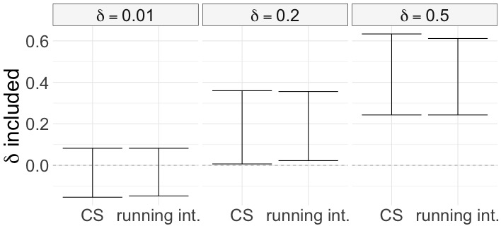
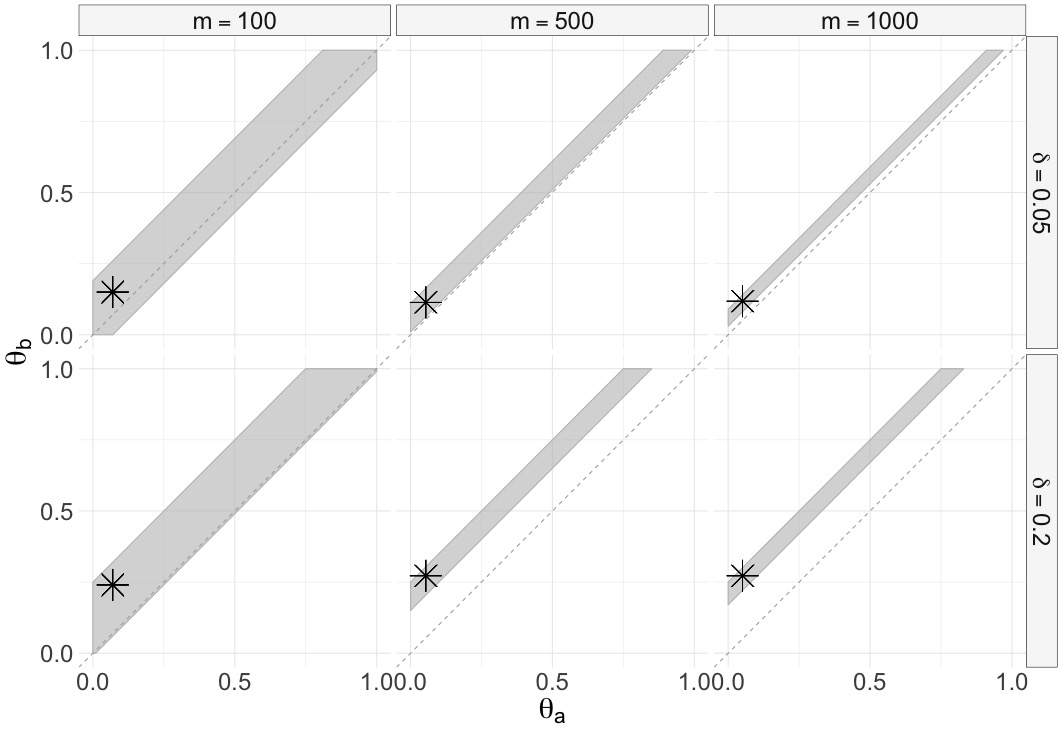
Risk difference is defined as the difference between success probabilities in the two streams: . Figure 2 shows running intersections of confidence sequences with as the risk difference for simulations for various distributions and stream lengths. These sequences are constructed by testing null hypotheses based on , with and . for the risk difference on is an interval, corresponding to the ‘beam’ of bounded by the lines and with being values such that . Figure B.1 in the Appendix illustrates that the running intersection indeed improves the confidence sequence, albeit slightly.
Relative risk
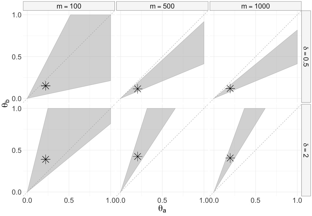
Relative risk is defined as the ratio between the success probabilities in group and : . Hence, confidence sequences for this effect size measure can again be constructed using the linear boundary form again, but now with and . Figure 2 shows running intersections of confidence sequences with as the relative risk.
Log odds ratio boundary
If the maximum likelihood estimate based on lies in the upper left corner as in Figure 3(a), the confidence sets we get at time have a one-sided shape such as the shaded region, or the shaded region in Figure 3(c), if the estimate lies in the lower right corner. Again, we can improve these confidence sequences by taking the running intersection; running intersections over time are illustrated in Figures 3(b) and 3(d).


4 Conclusion
We have shown how -variables for data streams can be extended to general null hypotheses and non-asymptotic always-valid confidence sequences. We specifically implemented the confidence sequences for the contingency tables setting; the resulting confidence sequences are efficiently computed and show quick convergence in simulations. For estimating risk differences or relative risk ratios between proportions in two groups, to our knowledge, such exact confidence sequences did not yet exist. For the log odds ratio we could also have used the sequential probability ratio (SPR) in Wald’s SPR test (Wald 1945) test, which can be re-interpreted as a (product of) -variables (Grünwald et al. 2022). However, the SPR does not satisfy the GRO property making it sub-optimal (see also (Adams 2020)); moreover, as should be clear from the development, our method for constructing confidence sequences can be implemented for any effect size notion with convex rejection sets and , not just the log odds ratio. A main goal for future work is to use Theorem 2 to provide such sequences for sequential two-sample settings that go beyond the table.
Acknowledgements
Funding: this work is part of the Enabling Personalized Interventions (EPI) project, which is supported by the Dutch Research Council (NWO) in the Commit2 - Data –Data2Person program under contract 628.011.028. Declarations of interest: none.
References
- Adams (2020) Reuben Adams. Safe hypothesis tests for 2 x 2 contingency table. Master’s thesis, Delft Technical University, 2020.
- Darling and Robbins (1967) D.A. Darling and H. Robbins. Confidence sequences for mean, variance, and median. Proc. National Academy of Sciences USA, 58(1):66, 1967.
- Grünwald et al. (2022) Peter Grünwald, Rianne de Heide, and Wouter Koolen. Safe testing. accepted, pending minor revision, for publication in Journal of the Royal Statistical Society: Series B, 2022.
- Henzi and Ziegel (2021) Alexander Henzi and Johanna F. Ziegel. Valid sequential inference on probability forecast performance. Biometrika, 2021.
- Howard et al. (2021) Steven R Howard, Aaditya Ramdas, Jon McAuliffe, and Jasjeet Sekhon. Uniform, nonparametric, non-asymptotic confidence sequences. Annals of Statistics, 2021.
- Li (1999) J.Q. Li. Estimation of Mixture Models. PhD thesis, Yale University, New Haven, CT, 1999.
- Ly et al. (2022) Alexander Ly, Rosanne Turner, and Judith Ter Schure. R-package safestats, 2022. CRAN.
- Shafer (2021) Glenn Shafer. The language of betting as a strategy for statistical and scientific communication. Journal of the Royal Statistical Society, Series A, 2021.
- Turner et al. (2021) Rosanne Turner, Alexander Ly, and Peter Grünwald. Generic e-variables for exact sequential k-sample tests that allow for optional stopping. arXiv preprint arXiv:2106.02693, 2021.
- Vovk and Wang (2021) Vladimir Vovk and Ruodu Wang. E-values: Calibration, combination, and applications. Annals of Statistics, 2021.
- Wald (1945) Abraham Wald. Sequential tests of statistical hypotheses. The Annals of Mathematical Statistics, 16(2):117–186, 1945.
Appendix A Proofs
Both proofs below use Theorem 1 of Grünwald et al. 2022 and a direct corollary (called Corollary 2 by Grünwald et al. 2022), which we re-state here, for convenience, combined as a single statement. Recall that we use notation .
Theorem (Theorem 1 of Grünwald et al. 2022)
Let be a random variable taking values in a set . Suppose is a probability distribution for with density that is strictly positive on all of and let be a set of distributions for where each has density . Let be the set of all distributions on . Assume . Then (a) there exists a (potentially sub-) distribution with density such that
is an -variable ( is called the Reverse Information Projection (RIPr) of onto ). Moreover, (b), satisfies
| (13) |
(where is the set of all -variables relative to null hypothesis ) and is thus the -GRO -variable for . If the minimum is achieved by some , i.e. , then . Moreover, (c), if there exists an -variable of the form for some then must achieve the infimum in (13) and must be essentially equal to in the sense that for all , . Similarly (d), if there exists a that achieves the infimum in (13) then is an -variable and is again essentially equal to .
Proof of Theorem 1
Part 1 The real idea behind the proof is the formulation of the modified testing problem in which only a single outcome per block is observed. This we already did in the main text. Linking the two is simply the last, very simple step, with analogies to the proof of Part 1 of Theorem 1 in Turner et al. 2021.
Let and let . Suppose that . Then , which follows immediately from applying Young’s inequality to but can also be derived directly by writing as function of and differentiating to .
Further, by independence, for ,
| (14) |
Combining the two facts stated above, (6) implies that the latter quantity is bounded by 1.
Part 2 By lower-semicontinuity of the KL divergence in its second argument (Posner’s theorem, used as in Grünwald et al. 2022) the infimum in (4) is achieved by some prior distribution so that by Theorem 1 of Grünwald et al. 2022 (part (b) in the formulation above), and hence also . By convexity of and finiteness of the support of , there must be some such that and hence also , which shows (a). This means that we have now created an -variable for the original problem which can be written as with a prior distribution on (namely, the one that puts mass on ). (b) is then an immediate consequence of Theorem 1 of Grünwald et al. 2022 (part (c) in the formulation above). (note that we cannot draw this conclusion if is not convex; for then the distribution may not correspond to the distribution in the original problem — this correspondence is only guaranteed if coincides with some .
Proof of Theorem 2
Recall that we assume that is convex and compact. We set where is the KL divergence as in (5), i.e. for the modified setting in which is a distribution on a single outcome, as discussed before Theorem 1. For the model this KL divergence can be written explicitly as
| (15) |
From (8) we now see that . We will prove the theorem with kl replaced by and by ; since the two KL’s agree up to a constant factor of , all results transfer to the kl mentioned in the theorem statement.
Since is compact in the Euclidean topology and all distributions in can be represented as 2-dimensional vectors, i.e. they have common and finite support, we must have that is compact in the weak topology so we can use the lower-semicontinuity of KL divergence in its second argument (Posner’s theorem) as in (Grünwald et al. 2022) to give us that the minimum KL divergence is achieved by some . Since KL divergence is strictly convex in its second argument and is convex (this is the place where we need to use rather than kl: may not be convex!), the minimum must be achieved uniquely. Since KL divergence is nonnegative and only if , it follows that if . Otherwise, since we assume to be in the interior of , iff lies on the boundary of . Thus, must lie in the interior of as well. cannot lie in the interior of though: for any point in the interior of we can draw a line segment between this point and . Differentiation along that line gives that monotonically decreases as we move towards , so the minimum within the closed set must lie on its boundary.
It remains to show that (9) is the -GRO -variable relative to . To see this, note that, by convexity of , from Theorem 1, we must have that the GRO -variable for this original problem is of the form
for some . The result then follows again by Theorem 1 of Grünwald et al. 2022 (part (c) in the formulation above): this shows that the distribution that puts mass 1 on minimizes, among all distributions on , . Since the set of such distributions includes all distributions that put mass on some , we must have that .
Appendix B Extended simulation results