The price of unfairness in linear bandits with biased feedback

Solenne Gaucher Thanks: solenne.gaucher@math.u-psud.fr Affiliation: Laboratoire de Mathématiques d’Orsay, Université Paris-Saclay Alexandra Carpentier Affiliation: University of Potsdam Christophe Giraud Affiliation: Laboratoire de Mathématiques d’Orsay, Université Paris-Saclay

Abstract

In this paper, we study the problem of fair sequential decision making with biased linear bandit feedback. At each round, a player selects an action described by a covariate and by a sensitive attribute. The perceived reward is a linear combination of the covariates of the chosen action, but the player only observes a biased evaluation of this reward, depending on the sensitive attribute. To characterize the difficulty of this problem, we design a phased elimination algorithm that corrects the unfair evaluations, and establish upper bounds on its regret. We show that the worst-case regret is smaller than $\mathcal{O}(\kappa_{*}^{1/3}\log(T)^{1/3}T^{2/3})$ , where $\kappa_{*}$ is an explicit geometrical constant characterizing the difficulty of bias estimation. We prove lower bounds on the worst-case regret for some sets of actions showing that this rate is tight up to a possible sub-logarithmic factor. We also derive gap-dependent upper bounds on the regret, and matching lower bounds for some problem instance. Interestingly, these results reveal a transition between a regime where the problem is as difficult as its unbiased counterpart, and a regime where it can be much harder.

1 Introduction

Artificial intelligence is increasingly used in a wide range of decision making scenarii with higher and higher stakes, with application in online advertisement [27], credit [3], health care [10], education [24] and job interviews [30], in the hope of improving accuracy and efficiency. Recent works have shown that the decisions made by algorithms can be dangerously biased against certain categories of people, and have endeavored to mitigate this behavior [19, 12, 6, 23]. Studies have underlined that the main cause of algorithmic unfairness is the presence of bias in the training set [23], which led to the development of methods aiming to guarantee the fairness of the algorithms. This paper, in lines with these works, addresses the problem of online decision making under biased feedback.

Linear bandits have become a very popular tool in online decision making problems, when side information on the actions is available in the form of covariates. In the present paper, we consider a variant of this problem, where the agent only has access to an unfair assessment of the action taken, that is systematically biased against a group of actions. For example, examiners may be prejudiced against people from a minority group, and give them lower grades; similarly, algorithms trained on biased data may produce unfair assessments of the credit risk of individuals belonging to a minority group. Note that not correcting biased evaluation can have adverse effects for all parties: on the one hand, actions disadvantaged by the evaluation mechanism will be unfairly discriminated against; on the other hand, the agent may spend his budget on an unfairly advantaged action that is actually sub-optimal. The problem of sequential decision making under biased feedback can be formalized as follows.

Biased linear bandit problem

A player is presented with a set of $k$ distinct actions characterized by covariates $x\in\mathcal{X}\subset\mathbb{R}^{d}$ , and by known sensitive attributes $z_{x}\in\{-1,1\}$ indicating the group of the action. At each round $t\leq T$ , the player chooses the action $x_{t}$ and receives an unobserved reward $x_{t}^{\top}\gamma^{*}$ , where $\gamma^{*}\in\mathbb{R}^{d}$ is the regression parameter specifying the true value of the action. The regret of the player is given by

R_{T}=\mathbb{E}\Big[\sum_{t\leq T}(x^{*}-x_{t})^{\top}\gamma^{*}\Big],\quad\text{ where }\quad x^{*}\in\argmax_{x\in\mathcal{X}}x^{\top}\gamma^{*}.

(1)

By contrast to the classical linear bandit, the player does not observe a noisy version of the unbiased reward $x_{t}^{\top}\gamma^{*}$ . Instead, she observes an unfair evaluation $y_{t}$ of the value of the action $x_{t}^{\top}\gamma^{*}$ , given by the following biased linear model:

y_{t}=x_{t}^{\top}\gamma^{*}+z_{x_{t}}\omega^{*}+\xi_{t}

where $\xi_{t}\overset{i.i.d}{\sim}\mathcal{N}(0,1)$ is a noise term. The evaluation are systematically biased against a certain group: this unequal treatment of the groups is captured by the bias parameter $\omega^{*}\in\mathbb{R}$ .

Preliminary discussion

The biased linear bandit is a variant of the linear bandit. By contrast, in the classical linear bandit model, the agent observes a noisy version of the reward. Obviously, applying directly an algorithm designed for linear bandit to biased linear bandits without correcting the evaluations would lead to a linear regret if the evaluation mechanism is prejudiced against the group of the best action in terms of reward, and if the best action in terms of feedback belongs to the advantaged group. To avoid this pitfall, one must estimate the bias in order to correct the evaluations. This implies a change in the exploration-exploitation trade-off, as exploration becomes more expensive. Indeed, in classical bandit problems, one can compare the rewards of two actions by repeatedly sampling them - or, to put it differently, one can find the best action by sampling only those actions that seem optimal. This does not hold in the biased linear bandit: if, at some point, the set of potentially optimal actions contains representatives from both groups, and does not span $\mathbb{R}^{d}$ , one is forced to sample sub-optimal actions to estimate the bias and improve the estimation of the unbiased rewards. For this reason, classical algorithm for linear bandit that only sample actions considered as potentially optimal, such as OFUL [1] or Phase Elimination [21], can suffer linear regret. This underlines the necessity to ensure sufficient estimation of the bias parameter, even when it implies sampling sub-optimal actions.

1.1 Related work

Fairness in bandit problems has mostly been studied from the perspective of fair budget allocation between actions. This problem is motivated by the fact that classical bandit algorithms select sub-optimal actions only a vanishing fraction of the time, which may be undesirable in many situations. To mitigate this problem and guarantee diversity in the actions selected, some papers [4, 25, 8, 13, 34] have proposed new algorithms ensuring fairness of the selection frequency of each action. The framework studied in this paper is different: we consider here that the mechanism for observing the rewards is unfair, and we aim at correcting it in order to maximize a (fair) true cumulative reward.

The biased linear model has been studied in the batch setting in [7], where the authors investigate the optimal trade-off between minimax risk and Demographic Parity. Detection of systematic bias, interpreted as a treatment effect, has been investigated in a batch setting in [15]. In [2], the authors consider a similar model, with unobserved sensitive attribute $z$ and known bias parameter $\omega^{*}$ , under additional assumption that the sensitive attribute $z$ is independent from the covariate $x$ . By contrast, we show that bias estimation is one of the main difficulties of the biased bandit problem.

The linear bandit with biased feedback can be viewed as a stochastic partial monitoring game. With the terminology of partial monitoring, the biased problem considered in the present paper is globally observable but not locally observable: in this case, the optimal worst-case regret rate typically increases as $\tilde{O}(T^{2/3})$ . This regret rate is for example achieved in the related problem of partial linear monitoring with linear feedback and linear reward using an Information Directed Sampling algorithm [17]. However, the dependence of the regret on the geometry of the action set and on the dimension $d$ remains in most cases an open question [22, 5, 17]. In this paper, we characterize the geometry of the biased linear bandit problem, and we investigate dependence of the regret on the gaps.

1.2 Contribution and outline

In this paper, we introduce the linear bandit problem with biased feedback. We design a new algorithm based on optimal design for this problem. We derive an upper bound on the worst case regret of this algorithm of order $\kappa_{*}^{1/3}\log(T)^{1/3}T^{2/3}$ for large $T$ , where $\kappa_{*}$ is an explicit constant depending on the geometry of the action set. We provide matching lower bounds on some problem instances, showing that the constant $\kappa_{*}$ characterizes the difficulty of the action set. Note that this regret is higher than the classical rates of order $\tilde{O}(dT^{1/2})$ obtained for $d$ -dimensional linear bandits: this increase corresponds to the price to pay for debiasing the unfair evaluations.

We also characterize the gap-depend regret, showing that it is of order $\left(\nicefrac{{d}}{{\Delta_{\min}}}\vee\nicefrac{{\kappa(\Delta)}}{{\Delta_{\neq}^{2}}}\right)\log(T)$ , where $\Delta_{\min}$ is the minimum gap, $\Delta_{\neq}$ is the gap between the best actions of the two groups, and $\kappa(\Delta)$ corresponds to the minimum regret to pay for estimating the bias with a given variance. This bound underlines the relative difficulties of the $d$ -dimensional linear bandit and of the bias estimation. When $\nicefrac{{d}}{{\Delta_{\min}}}\geq\nicefrac{{\kappa(\Delta)}}{{\Delta_{\neq}^{2}}}$ , i.e. when one group contains all near-optimal actions, the difficulty is dominated by that of the corresponding linear bandit problem. When both groups contain near-optimal actions, and $\nicefrac{{d}}{{\Delta_{\min}}}\leq\nicefrac{{\kappa(\Delta)}}{{\Delta_{\neq}^{2}}}$ , the regret corresponds to the price of debiasing the rewards.

The rest of the paper is organized as follows. In Section 2, we present the Fair Phased Elimination algorithm: we first discuss parameter estimation in Section 2.1, before presenting a sketch of the algorithm in Section 2.2 (a detailed version of this algorithm is provided in Appendix B). Then, in Section 3, we establish an upper bound on its worst-case regret. In Section 4, we derive a gap-dependent upper bound on the regret of our algorithm. In Section 5, we establish lower bounds on some action sets for both the worst-case and the gap-dependent regret, showing that these rates are sharp respectively up to a sub-logarithmic factor and an absolute multiplicative constant. Additional discussions on the geometry of bias estimation are postponed to Appendix A.

1.3 Notations and additional assumptions

We assume that all covariates $x\in\mathcal{X}$ are distinct, which implies that the group $z_{x}$ of action $x$ is well defined. We also assume that no group is empty, that the set $\{\left({x\atop z_{x}}\right)\ :\ x\in\mathcal{X}\}$ spans $\mathbb{R}^{d+1}$ (which guarantees identifiability of the parameters), and that the rewards are bounded: $\max_{x\in\mathcal{X}}|x^{\top}\gamma^{*}|\leq 1$ .

When necessary, we underline the dependence of the regret on the parameter $\theta$ by denoting it $R_{T}^{\theta}$ . We denote by $a_{x}=\left({x\atop z_{x}}\right)$ the vector describing an action and its group, by $\theta^{*}=\left({\gamma^{*}\atop\omega^{*}}\right)\in\mathbb{R}^{d+1}$ the unknown parameter, and by $\mathcal{A}=\left\{a_{x}:x\in\mathcal{X}\right\}$ the set of actions and of corresponding sensitive attributes. We denote by $\Delta=(\Delta_{x})_{x\in\mathcal{X}}$ the vector of gaps $\Delta_{x}=\max_{x^{\prime}\in\mathcal{X}}(x^{\prime}-x)^{\top}\gamma^{*}$ , and by $\mathcal{C}(\mathcal{X})=\left\{\gamma\in\mathbb{R}^{d}:\forall x\in\mathcal{X},|x^{\top}\gamma|\leq 1\right\}$ the set of admissible parameters. Note that for all $x\in\mathcal{C}(\mathcal{X})$ , $\Delta_{x}\leq 2$ . For $i\leq d+1$ , let $e_{i}$ be the $i$ -th vector of the canonical basis of $\mathbb{R}^{d+1}$ , and for any matrix $M$ , let $M^{+}$ be a generalized inverse of $M$ . We denote by $\mathcal{P}^{\mathcal{X}}$ the set of probability measures on $\mathcal{X}$ , and $\mathcal{M}^{\mathcal{X}}=\{\mu:\mathcal{X}\mapsto\mathbb{R}_{+}\}$ . For any $\mu\in\mathcal{P}^{\mathcal{X}}$ or $\mu\in\mathcal{M}^{\mathcal{X}}$ , we denote $V(\mu)=\sum_{x\in\mathcal{X}}\mu(x)a_{x}a_{x}^{\top}$ the covariance matrix corresponding to this allocation. Moreover, for $u\in\mathbb{R}^{d+1}$ (resp. $\mathcal{U}\in\mathbb{R}^{d+1}$ ), we denote by $\mathcal{P}^{\mathcal{X}}_{u}$ (resp. $\mathcal{M}^{\mathcal{X}}_{u}$ ) the measures $\mu$ in $\mathcal{P}^{\mathcal{X}}$ (resp. in $\mathcal{M}^{\mathcal{X}}$ ) such that $u\in\Image(V(\mu))$ . For $\mathcal{U}\subset\mathbb{R}^{d+1}$ , we denote by $\mathcal{P}^{\mathcal{X}}_{\mathcal{U}}$ (resp. $\mathcal{M}^{\mathcal{X}}_{\mathcal{U}}$ ) the measures $\mu$ such that $\mu\in\mathcal{P}^{\mathcal{X}}_{u}$ (resp. $\mathcal{M}^{\mathcal{X}}_{u}$ ) for all $u\in\mathcal{U}$ .

2 Fair Phased Elimination algorithm

The Fair Phased Elimination algorithm belongs to the category of sequential elimination algorithms. Classical sequential elimination algorithms typically proceed by phases, indexed by $l=1,2,\ldots$ . At phase $l$ , these algorithms consider a set of potentially optimal actions $\mathcal{X}_{l}$ . The rewards of all actions $x\in\mathcal{X}_{l}$ are then estimated with a given precision $O(\epsilon_{l})$ , typically chosen as $\epsilon_{l}=2^{2-l}$ , by sampling actions in $\mathcal{X}_{l}$ . Actions sub-optimal by a gap larger than the precision level are then removed from the set $\mathcal{X}_{l+1}$ of potentially optimal actions for the phase $l+1$ .

As underlined previously, sequential elimination algorithms may suffer linear regret in the biased linear bandit problem if actions allowing to estimate the bias are discarded by the algorithm before the best group is identified. To mitigate this problem, we first estimate the biased evaluations of the potentially optimal actions, using ordinary least squares estimation. We then debias the estimations using an estimator for the bias relying on independent observations, which may be obtained by sampling sub-optimal actions. Before presenting the algorithm, let us discuss the estimation of the evaluations and of the bias parameter.

2.1 Optimal design for parameter estimation in the biased linear bandit

G-optimal design for biased evaluation estimation

As in the Phased Elimination algorithm [21], we rely on G-optimal design to estimate the biased evaluations $a_{x}^{\top}\theta^{*}$ with small error uniformly over a set of actions $\mathcal{X}_{l}$ . More precisely, for a given set of potentially optimal actions $\mathcal{X}_{l}$ , we compute the G-optimal design solution to the problem

\underset{\pi\in\mathcal{P}_{\mathcal{X}_{l}}^{\mathcal{X}_{l}}}{\minimize}\ \underset{x\in\mathcal{X}_{l}}{\max}\ a_{x}^{\top}\left(V(\pi)\right)^{+}a_{x}\ .\ \ \ \ \ \ \ \ \ \ \ \ \ \ \text{(G-optimal design)}

(2)

This can be done using polynomial-time algorithms, relying for example on interior points method [32], or on mixed integer second-order cone programming [31]. The celebrated General Equivalence theorem of Kiefer [16] and Pukelsheim [29] states that the value of Equation (2) is bounded by $d+1$ . Let $\pi^{*}$ denote any design solution to the G-optimal design problem (2), and let $\widehat{\theta}$ denote the ordinary least square estimator obtained by sampling each action $x\in\mathcal{X}_{l}$ exactly $\left\lceil n\pi^{*}(x)\right\rceil$ times for a given $n>0$ . Then, for all $x\in\mathcal{X}_{l}$ , the General Equivalence theorem implies that the variance of the estimate $a_{x}^{\top}\widehat{\theta}$ is smaller than $\nicefrac{{(d+1)}}{{n}}$ . Moreover, the G-optimal design $\pi^{*}$ can be chosen so that it is supported by at most $\nicefrac{{(d+1)(d+2)}}{{2}}$ points, so the total number of samples is at most $n+\nicefrac{{(d+1)(d+2)}}{{2}}$ .

$\Delta$ -optimal design for bias evaluation

In this paragraph, we introduce the $\Delta$ -optimal design, which is discussed in greater depth in Appendix A.5. To estimate the bias parameter $\omega^{*}$ , we use the estimator $\widehat{\omega}=e_{d+1}^{\top}\widehat{\theta}$ , where $\widehat{\theta}$ is the ordinary least square estimator for the full parameter $\theta^{*}$ . Now, if we sample each action $x\in\mathcal{X}$ exactly $\mu(x)$ time, the variance of $\widehat{\omega}$ is equal to $e_{d+1}^{\top}V(\mu)^{+}e_{d+1}$ . Given the vector of gaps $\Delta$ , the design $\mu$ minimizing the regret of this exploration phase, while ensuring that the variance of $\widehat{\omega}$ is smaller than $1$ , is solution of the problem

\displaystyle\underset{\mu\in\mathcal{M}_{\mathcal{X}}^{e_{d+1}}}{\minimize}\ \sum_{x}\mu(x)\Delta_{x}\quad\text{such that }\quad e_{d+1}^{\top}V(\mu)^{+}e_{d+1}\leq 1.\quad\text{ ($\Delta$-optimal design)}

(3)

Let us denote $\mu^{\Delta}$ a minimizer of (3), and $\kappa(\Delta)={\sum}_{x\in\mathcal{X}}\mu^{\Delta}(x)\Delta_{x}$ . Lemma 9 in Appendix A explains how to compute the design $\mu^{\Delta}$ in polynomial time by adapting tools from $c$ -optimal design. This lemma also shows that the support of $\mu^{\Delta}$ can be chosen to be of cardinality at most $d+1$ . Then, choosing each action exactly $\lceil n\mu^{\Delta}(x)\rceil$ times for a given $n>0$ allows us to estimate the bias with variance lower than $n^{-1}$ and a regret no larger than $n\kappa(\Delta)+2(d+1)$ . Obviously, we do not know the gap vector $\Delta$ beforehand, so we must estimate it as we go.

2.2 Outline of the Fair Phased Elimination algorithm

The Fair Phased Elimination algorithm, sketched in Algorithm 3, relies on the following key ideas. First, note that within a group, the order of the true rewards and of the biased evaluations are the same. Hence, within a group, we can use classical algorithms for linear bandits to choose the actions and estimate the biased evaluations with a controlled within-group regret: this is done using $\mathbf{G}$ -exploration and elimination. Second, to compare actions belonging to different groups, we independently estimate the bias parameter $\omega^{*}$ , using $\mathbf{\Delta}$ -exploration and elimination. Finally, we underline that bias estimation may require to sample very sub-optimal actions. Therefore, it can be overly costly to estimate the bias up to the precision level required to identify the best group. To prevent this, we use a stopping criteria.

G-exploration and elimination

At each phase $l=1,2,...$ , we keep two sets of potentially optimal actions belonging to the groups $+1$ and $-1$ , denoted respectively $\mathcal{X}_{l}^{(+1)}$ and $\mathcal{X}_{l}^{(-1)}$ . If we have not identified the group containing the best action, we run a G-Exp-Elim routine 1 on each set $\mathcal{X}_{l}^{(z)}$ for $z=1$ and $z=-1$ . This routine samples actions according to a rounded G-optimal design on $\mathcal{X}_{l}^{(z)}$ , with a total number of observations chosen so that the biased evaluations of all actions in $\mathcal{X}_{l}^{(z)}$ are known with an error at most $\epsilon_{l}$ . The set $\mathcal{X}_{l+1}^{(z)}$ is obtained by removing from $\mathcal{X}_{l}^{(z)}$ actions whose estimated evaluations are sub-optimal by a gap larger than $3\epsilon_{l}$ , compared to the empirical best action in the group. This allows to ensure that only actions sub-optimal by a gap $\mathcal{O}(\epsilon_{l})$ remain in $\mathcal{X}_{l+1}^{(z)}$ , and to estimate the gap vector $\Delta$ with a precision sufficient for $\Delta$ -optimal estimation.

If the group containing the best action has been identified, we discard the other group, and run a G-Exp-Elim routine 1 on the set of potentially optimal actions in this group.

Routine 1 G-Exp-Elim (

\mathcal{X},n,\epsilon

)

1: Compute G-optimal design

\pi

solution of (2) on

\mathcal{X}

, with

|\supp(\pi)|\leq\nicefrac{{(d+1)(d+2)}}{{2}}

2: Sample

\left\lceil n\pi(x)\right\rceil

times each action

a_{x}

for

x\in\mathcal{X}

\triangleright

G-optimal parameter estimation

3: Compute the ordinary least square estimator

\widehat{\theta}

\mathcal{X}^{{}^{\prime}}\leftarrow\left\{x\in\mathcal{X}:\max_{x^{\prime}\in\mathcal{X}}(x^{\prime}-x)^{\top}\widehat{\theta}\leq 3\epsilon\right\}

\triangleright

Suboptimal actions elimination

5: return

\widehat{\theta}

and

\mathcal{X}^{\prime}

$\Delta$ -exploration and elimination

If the group of the best action has not been found before phase $l$ , we run the $\Delta$ -Exp-Elim routine 2. More precisely, relying on a previous estimate $\widehat{\Delta}^{l}$ of the gap vector $\Delta$ , we compute the $\widehat{\Delta}^{l}$ -optimal design $\widehat{\mu}$ . We then estimate the bias using actions sampled according to a rounded version of this design, with a total number of observations chosen so that the error of bias estimation is smaller than $\epsilon_{l}$ , and use it to debias the reward estimation. If the debiased evaluation of the best action of each group are separated by a gap larger than $4\epsilon_{l}$ , we consider that the best group is the one containing the empirical best action in terms of biased evaluation, and we discard the other group.

If we cannot find the best group, we rely on estimates of the bias and of the biased evaluations obtained during the previous round to update the estimate of the gap vector $\widehat{\Delta}^{l+1}$ .

Routine 2

\Delta

-Exp-Elim (

\mathcal{X},(\mathcal{X}^{(z)},\widehat{\theta}^{(z)})_{z\in\left\{-1,1\right\}},\widehat{\Delta},n,\epsilon

)

1: Compute

\widehat{\Delta}

-optimal design

\big(\hat{\mu},\kappa(\hat{\Delta})\big)

solution of (3) on

\mathcal{X}

, with

|\supp(\hat{\mu})|\leq d+1

2: Sample

\left\lceil n\hat{\mu}(x)\right\rceil

times each action

a_{x}

for

x\in\mathcal{X}

\triangleright

\widehat{\Delta}

-optimal bias estimation

3: Compute

\mbox{${\widehat{\omega}}$}=e_{d+1}^{\top}\widehat{\theta}

, where

\widehat{\theta}

is the ordinary least square estimator

4: for

z\in\left\{-1,1\right\}

and

x\in\mathcal{X}^{(z)}

\widehat{m}_{x}\leftarrow a_{x}^{\top}\widehat{\theta}^{(z)}-z\mbox{${\widehat{\omega}}$}

\triangleright

Debiased rewards estimation

5: if

\exists z\in\left\{-1,1\right\}

such that

\displaystyle{\max_{x\in\mathcal{X}^{(z)}}\widehat{m}_{x}\geq\max_{x\in\mathcal{X}^{(-z)}}\widehat{m}_{x}+4\epsilon}

then

\mathcal{Z}\leftarrow\left\{z\right\}

\triangleright

Group elimination

6: else

\widehat{\Delta}_{x}\leftarrow 2\wedge\left(\max_{x^{\prime}\in\mathcal{X}^{(-1)}\cup\mathcal{X}^{(1)}}\widehat{m}_{x^{\prime}}-\widehat{m}_{x}+4\epsilon\right)

for all

x\in\mathcal{X}^{(-1)}\cup\mathcal{X}^{(1)}

7: return

\mathcal{Z}

and

\widehat{\Delta}

Stopping criteria

As underlined previously, the $\Delta$ -Exp-Elim routine samples actions that can be very sub-optimal. As a consequence, when the gap between the best two actions of each group is small, finding the best group can be overly costly in terms of regret. To prevent this, if the best group has not been found at stage $l$ fulfilling $\epsilon_{l}\leq\big(\nicefrac{{\kappa(\widehat{\Delta}^{l})\log(T)}}{{T}}\big)^{1/3}$ , the bias estimation is stopped and the empirical best action in $\mathcal{X}^{(1)}_{l+1}\cup\mathcal{X}^{(-1)}_{l+1}$ is sampled for the remaining time (see Algorithm 3)

Algorithm 3 Fair Phased Elimination (sketched)

1: input:

\delta

T

\mathcal{X}

k=|\mathcal{X}|

\epsilon_{l}=2^{2-l}

for

l\geq 1

2: initialize:

\mathcal{X}_{1}^{(+1)}\leftarrow\{x:z_{x}=1\}

\mathcal{X}_{1}^{(-1)}\leftarrow\{x:z_{x}=-1\}

\mathcal{Z}_{1}\leftarrow\{-1,+1\}

\widehat{\Delta}^{1}\leftarrow\left(2,...,2\right)

l\leftarrow 0

4: while the budget is not spent do

l\leftarrow l+1

5: for

z\in\mathcal{Z}_{l}

\left(\widehat{\theta}^{(z)},\mathcal{X}_{l+1}^{(z)}\right)\leftarrow\textsc{G-Exp-Elim}\left(\mathcal{X}_{l}^{(z)},{2(d+1)\over\epsilon_{l}^{2}}\log\left(\frac{kl(l+1)}{\delta}\right),\epsilon_{l}\right)

7: if

\mathcal{Z}_{l}=\{-1,+1\}

then

8: if

\epsilon_{l}\leq\left(\kappa(\widehat{\Delta}^{l})\log(T)/T\right)^{1/3}

then

\triangleright

Stop bias estimation

9: Sample best action in

\mathcal{X}_{l+1}^{(-1)}\cup\mathcal{X}_{l+1}^{(+1)}

for the remaining time

10: else

11:

\left(\mathcal{Z}_{l+1},\widehat{\Delta}^{l+1}\right)\leftarrow\Delta\textsc{-Exp-Elim}\left(\mathcal{X},\Big(\mathcal{X}^{(z)}_{l+1},\widehat{\theta}_{l}^{(z)}\Big)_{z\in\left\{-1,1\right\}},\widehat{\Delta}^{l},{2\over\epsilon_{l}^{2}}\log\left(\frac{l(l+1)}{\delta}\right),\epsilon_{l}\right)

3 Upper bound on the worst-case regret of Fair Phased Elimination

The regret of the Fair Phased Elimination depends on the difficulty of estimating the bias parameter, captured by $\kappa(\Delta)$ . Lemma 7 in Appendix A.5 shows that for all parameter $\gamma^{*}\in\mathcal{X}$ , $\kappa(\Delta)$ is upper bounded by $2\kappa_{*}$ , where $\kappa_{*}$ is the minimal variance of the bias estimator given by

\kappa_{*}=\underset{\pi\in\mathcal{P}^{\mathcal{X}}_{e_{d+1}}}{\min}\ e_{d+1}^{\top}\left(V(\pi)\right)^{+}e_{d+1}.

The following theorem provides a bound on the worst case regret depending on $\kappa_{*}$ . Proofs are postponed to Appendix C.1.

Theorem 1.

For the choice $\delta=T^{-1}$ , there exists two numerical constants $C,C^{\prime}>0$ such that the following bound on the regret of the Fair Phased Elimination algorithm 4 holds

	$\displaystyle R_{T}$	$\displaystyle\leq C\left(\kappa_{}^{1/3}T^{2/3}\log(T)^{1/3}+(d\vee\kappa_{})\log(T)+d^{2}+d\kappa_{*}^{-1/3}T^{1/3}\log(kT)\log(T)^{-1/3}\right)$
		$\displaystyle\leq C^{\prime}\kappa_{}^{1/3}T^{2/3}\log(T)^{1/3}\quad\quad\textrm{for}\quad T\geq\frac{\left((d\vee\kappa_{})^{3/2}\log(T)\right)\vee d^{3}}{\sqrt{\kappa_{}}}\vee\frac{(d\log(kT))^{3}}{(\kappa_{}\log(T))^{2}}.$

In Section 5.1, we show that the upper bound obtained in Theorem 1 is sharp in some settings, up to the sub-logarithmic factor $\log(T)^{1/3}$ .

Theorem 1 shows that the worst-case regret of the Fair Phased Elimination algorithm asymptotically grows as $C\kappa^{1/3}_{*}T^{2/3}\log\left(T\right)^{1/3}$ . This worst-case regret rate is higher than the typical rate $Cd\log(T)T^{1/2}$ obtained under unbiased feedback on the rewards (see, e.g., [1]). This increase in the regret corresponds to the cost of learning from unfair evaluations. It is due to the fact that the algorithm may need to sample actions that are sub-optimal in order to estimate the bias parameter. Note that this rate $\widetilde{\mathcal{O}}(T^{2/3})$ is typical for globally observable bandit problems with partial linear monitoring, and can be obtained by applying results established in [17] for in the partial linear monitoring setting to the biased linear bandit problem.

By contrast to previous results, Theorem 1 characterizes precisely the dependence of the worst-case regret on the geometry of the action set. The relevant constant $\kappa_{*}$ is the minimal variance for estimating the bias, which appears when considering the related $c$ -optimal design problem. While the connection between G-optimal design and the linear bandit problem has already been exploited, it is to the best of our knowledge the first time that $c$ -optimal design is related to a partial monitoring problem.

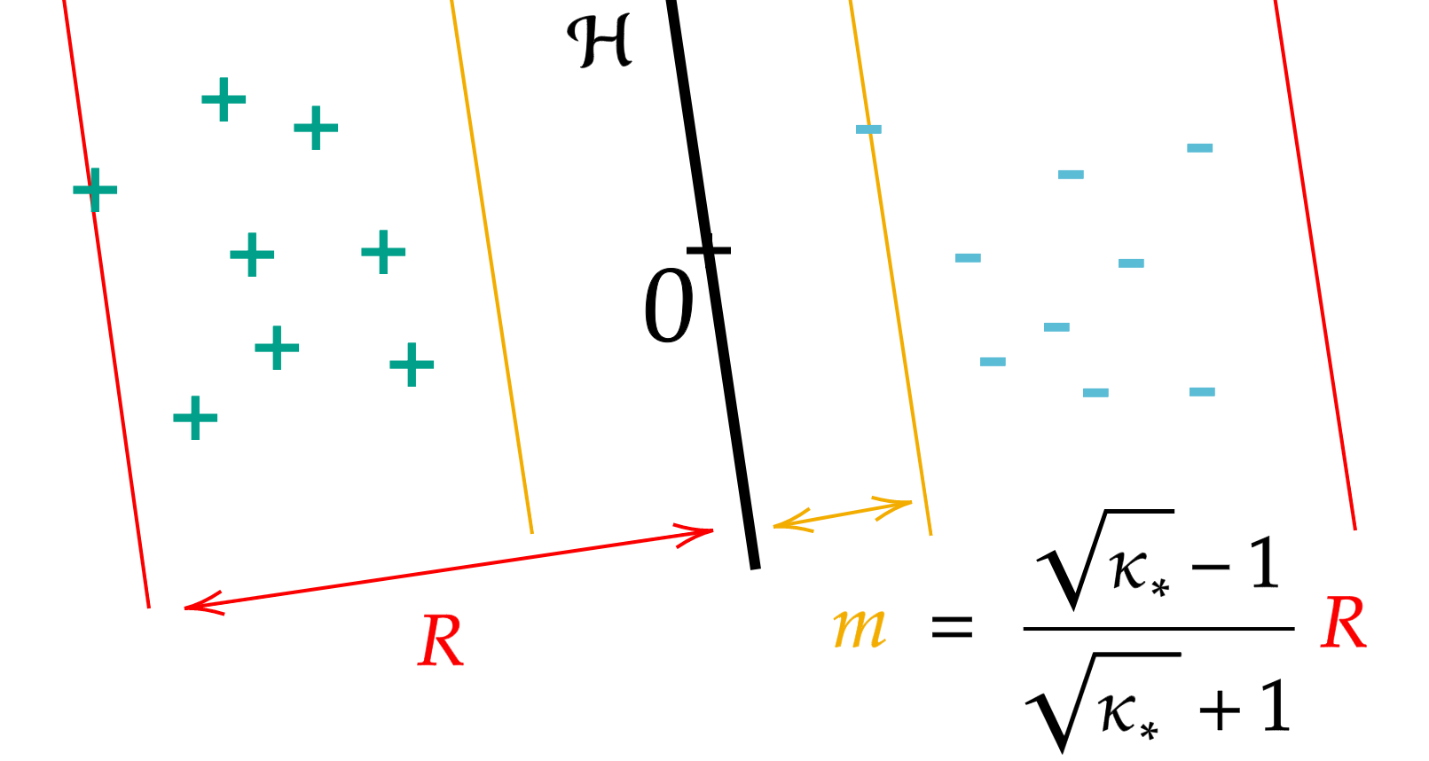
The constant $\kappa_{*}$ corresponds to the minimum number of samples required for estimating the bias with a variance equal to $1$ (up to rounding issues). Intuitively, if the actions are very correlated with their sensitive attributes, more samples will be needed to estimate the bias with the same precision. This situation corresponds to cases where $\kappa_{*}$ is large, and leads to a higher regret. Lemma 1, illustrated in Figure 1, relates $\kappa_{*}$ to the margin between the two groups of actions.

Lemma 1.

$\kappa_{*}$ is the largest constant $\kappa\geq 0$ such that, there exists an hyperplane $\mathcal{H}$ containing zero and separating the two groups, and such that, the margin to $\mathcal{H}$ is at least $\nicefrac{{\sqrt{\kappa}-1}}{{\sqrt{\kappa}+1}}$ times the maximum distance of all points to the hyperplane (see Figure 1). When no such hyperplane exists, then $\kappa_{*}=1$ .

Refer to caption — (a) The margin $m$ is equal to $\nicefrac{{\sqrt{\kappa_{*}}-1}}{{\sqrt{\kappa_{*}}+1}}$ times the maximum distance $R$ of any action to the hyperplane.

Interestingly, Lemma 1 underlines that under reasonable assumptions, the constant $\kappa_{*}$ may not depend on the ambient dimension $d$ , and it can even be equal to $1$ . By contrast, the previous bounds obtained for an Information Directed Sampling algorithm are of order $\alpha^{1/3}d^{1/2}T^{2/3}\log(kT)^{1/2}$ , where $\alpha$ is a measure of the complexity of the action set called the worst-case alignment constant. Lemma 6 in Appendix A shows that $\alpha$ is equivalent to the minimal variance of the bias estimator $\kappa_{*}$ . Hence, our bound improves over previous results by a factor $d^{1/2}\log(T)^{1/6}(\log(kT)/\log(T))^{1/2}$ .

The gaps are not involved in the definition of the minimal variance of bias estimation $\kappa_{*}$ . The reader may have expected to get, instead of $\kappa_{*}$ , the minimax regret for estimating the bias

\widetilde{\kappa}=\underset{\gamma\in\mathcal{C}(\mathcal{X}),x^{\prime}\in\mathcal{X}}{\max}\underset{x\in\mathcal{X}}{\sum}\widetilde{\mu}(x)(x^{\prime}-x)^{\top}\gamma,\quad\ \text{where}

\displaystyle\widetilde{\mu}=\underset{\mu}{\argmin}\underset{x^{\prime}\in\mathcal{X},\gamma\in\mathcal{C}(\mathcal{X})}{\max}\underset{x\in\mathcal{X}}{\sum}\mu(x)(x^{\prime}-x)^{\top}\gamma,\ \text{such that }\mu\in\mathcal{M}^{\mathcal{X}}_{e_{d+1}}\ \text{and }\ e_{d+1}^{\top}V(\mu)^{+}e_{d+1}\leq 1.

Next lemma shows that $\kappa_{*}$ and $\widetilde{\kappa}$ are in equivalent up to a factor 2. We refer the interested reader to Appendix A, where further discussions on the geometry of bias estimation are postponed, due to space constraints.

Lemma 2.

$\displaystyle\nicefrac{{\widetilde{\kappa}}}{{2}}\leq\kappa_{*}\leq 2\widetilde{\kappa}.$

4 Upper bound on the gap-depend regret of Fair Phased Elimination

In this section, we provide an upper bound on the worst-case regret that depends on the gap between the two best actions, and on the gap between the best actions of the two groups. Compared to instance-dependent bounds, established in the linear bandit problem in [20, 18], gap-dependent bounds characterize the dependence of the regret on a small number of parameters. They are typically less sharp than instance-dependent bounds, but allow to better highlight the influence of the parameters on the difficulty of the problem. The bound established in the following theorem relates the difficulty of the biased linear bandit to that of bias estimation, and to that of the corresponding $d$ -dimensional linear bandit. Proofs are postponed to Appendix C.1.

Theorem 2.

Assume that $x^{*}\in\argmax_{x\in\mathcal{X}}x^{\top}\gamma^{*}$ is unique. Then, there exists two numerical constants $C,C^{\prime}>0$ such that, for the choice $\delta=T^{-1}$ , the following bound on the regret of the Fair Phased Elimination algorithm 4 holds

	$\displaystyle R_{T}$	$\displaystyle\leq$	$\displaystyle C\left(\left(\frac{d}{\Delta_{\min}}\lor\frac{\kappa\big(\Delta\vee\Delta_{\neq}\vee\varepsilon_{T}\big)}{\Delta_{\neq}^{2}}\right)\log(T)+d^{2}+\frac{d}{\Delta_{\min}}\log\left(k\right)\right)$
		$\displaystyle\leq$	$\displaystyle C^{\prime}\left(\frac{d}{\Delta_{\min}}\lor\frac{\kappa\big(\Delta\vee\Delta_{\neq}\vee\varepsilon_{T}\big)}{\Delta_{\neq}^{2}}\right)\log(T)\quad\quad\textrm{for }\quad T\geq k\vee e^{d\Delta_{\min}}\$

where $\Delta_{\min}=\min_{x\in\mathcal{X}\setminus x^{*}}\Delta_{x}$ , $\Delta_{\neq}=\min_{x\in\mathcal{X}:z_{x}=-z_{x^{*}}}\Delta_{x}$ , and $\varepsilon_{T}=(\nicefrac{{\kappa_{*}\log(T)}}{{T}})^{1/3}.$

The term $\nicefrac{{d}}{{\Delta_{\min}}}\lor\nicefrac{{\kappa(\Delta\vee\Delta_{\neq}\vee\varepsilon_{T})}}{{\Delta_{\neq}^{2}}}$ highlights the two sources of difficulty of the problem. On the one hand, the term $\nicefrac{{d}}{{\Delta_{\min}}}$ is unavoidable: even if the algorithm knew beforehand the group containing the best action, it would still need to play a game of $d$ -dimensional linear bandits in this group, and suffer, in the worst-case, the corresponding gap-dependent regret [1]. Note that lower bounds on gap-depend regret of classical linear bandits follow from considering a setting with one near-optimal action with gap $\Delta_{\min}$ in each of the $d$ dimensions. Then, any algorithm needs to explore each dimension up to $\Delta_{\min}^{-2}\log(T)$ times in order to find the best action, but can do so by choosing the near-optimal actions, thus having a regret $\Delta_{\min}^{-1}\log(T)$ in each direction. By contrast, the term $\nicefrac{{\kappa(\Delta\vee\Delta_{\neq}\vee\varepsilon_{T})}}{{\Delta_{\neq}^{2}}}$ is characteristic of the biased linear bandit problem: it is due to the fact that the algorithm may need to sample very sub-optimal actions in order to find the group containing the best action. Indeed, to identify this group, one must estimate the bias with a precision $\Delta_{\neq}$ , i.e. sample sub-optimal actions with average regret $\kappa(\Delta)$ approximately $\Delta_{\neq}^{-2}\log(T)$ times.

When $\nicefrac{{d}}{{\Delta_{\min}}}\leq\nicefrac{{\kappa(\Delta\vee\Delta_{\neq}\vee\varepsilon_{T})}}{{\Delta_{\neq}^{2}}}$ , the regret corresponds to the regret of this bias estimation phase. In other words, when both groups contain near-optimal actions, the difficulty of the problem is dominated by the price to pay for debiasing the unfair evaluations. Interestingly, when $\nicefrac{{d}}{{\Delta_{\min}}}>\nicefrac{{\kappa(\Delta\vee\Delta_{\neq}\vee\varepsilon_{T})}}{{\Delta_{\neq}^{2}}}$ , the difficulty of the linear bandit with systematic bias is dominated by that of the classical $d$ -linear bandit. In this case, the algorithm is able to find the group containing the best action, and the problem reduces to a linear bandit in dimension $d$ . Thus, the linear bandit with systematic bias is a non trivial example of a globally observable game that can be locally observable around the best action.

Finally, we underline that the magnitude of the bias does not appear in the regret: intuitively, no matter its magnitude, the algorithm always need to estimate it up to the same precision (of order $\Delta_{\neq}$ ) in order to find the best group and to be optimal in terms of gap-depend regret. This indicates that our algorithm is robust against important discriminations in the evaluation mechanism.

5 Lower bounds on the regret

In this section, we derive lower bounds on the worst-case regret and the gap-dependent regret that respectively match the upper bounds established in Theorems 1 and 2 up to sub-logarithmic factors or numerical constants.

5.1 Lower bound on the worst-case regret

Theorems 1 and 2 underline the dependence of the regret on the geometry of the action set. Before stating our result, we begin by introducing the notion of $\kappa_{*}$ -correlated action set.

Definition 1 ( $\kappa_{*}$ -correlated action set).

For $\kappa_{*}\geq 1$ , a set of actions $\mathcal{A}$ is $\kappa_{*}$ -correlated if $\mathcal{A}\in\mathbf{A}_{\kappa_{*},d}$ , where

\mathbf{A}_{\kappa_{*},d}=\left\{\begin{tabular}[]{l}$\mathcal{A}=\left\{a_{1},...,a_{k}\right\}\subset\Big(\mathbb{R}^{d}\times\{-1,+1\}\Big)^{k}:$\\ $k\in\mathbb{N}^{*},\underset{\pi\in\mathcal{P}^{\mathcal{A}}_{e_{d+1}}}{\min}\left\{e_{d+1}^{\top}\Big(\underset{a\in\mathcal{A}}{\displaystyle\sum}\pi(a)aa^{\top}\Big)^{+}e_{d+1}\right\}\geq\kappa_{*}$\end{tabular}\right\}

is the set of actions sets such that the minimal variance of the bias estimator is larger than $\kappa_{*}$ .

In the following theorem, we establish a lower bound on the regret valid for all $\kappa_{*}\geq 1$ by designing $\kappa_{*}$ -correlated sets of actions $\mathcal{A}\in\mathbf{A}_{\kappa_{*},d}$ , and obtaining lower bounds on the regret of any algorithm on these sets of actions.

Theorem 3.

Let $\kappa_{*}\geq 1$ , $d\geq 2$ and $T\geq 4^{3}\kappa_{*}$ . There exists an action set $\mathcal{A}\in\mathbf{A}_{\kappa_{*},d}$ such that for any algorithm, there exists a bandit problem with parameter $\theta_{T}\in\mathbb{R}^{d+1}$ such that the regret of this algorithm on the problem characterized by $\theta_{T}$ satisfies $\displaystyle R_{T}^{\theta_{T}}\geq\nicefrac{{\kappa_{*}^{1/3}T^{2/3}}}{{8e}}.$

Previous lower bounds on the regret of linear bandits with partial monitoring, established in [17], state that the regret must be at least $c_{\mathcal{A}}T^{2/3}$ for some parameter $\theta_{T}\in\mathbb{R}^{d+1}$ , where $c_{\mathcal{A}}>0$ is a constant depending (not explicitly) on $\mathcal{A}$ . By contrast, Theorem 3 provides an explicit characterization of the dependence of the regret rate on the geometry of the problem, which matches the upper bound of Theorem 1 up to a sub-logarithmic factor. Note that the assumption $d\geq 2$ is necessary here: if $d=1$ , there are at most two potentially optimal actions (namely, $\max\{x:x\in\mathcal{X}\}$ and $\min\{x:x\in\mathcal{X}\}$ ). Then, the problem becomes locally observable, and regret of order $\widetilde{O}(T^{1/2})$ can be achieved [17].

5.2 Lower bound on the gap-dependent regret

We now present a lower bound on the gap-dependent regret. More precisely, for given values of $\Delta_{\min}$ and $\Delta_{\neq}$ , we establish a lower bound on the worst case regret among parameters $\theta$ verifying $\Delta_{\min}\leq\min_{x\in\mathcal{X}\setminus x^{*}}\Delta_{x}$ , and $\Delta_{\neq}\leq\min_{x\in\mathcal{X}:z_{x}=-z_{x^{*}}}\Delta_{x}$ . Before stating formally the result, let us define the corresponding parameter set. For an action set $\mathcal{A}\in\mathbf{A}_{\kappa_{*},d}$ , and for $\left(\Delta_{\min},\Delta_{\neq}\right)\in(0,1)^{2}$ such that $\Delta_{\min}\leq\Delta_{\neq}$ , we denote

\mathbf{\Theta}^{\mathcal{A}}_{\Delta_{\min},\Delta_{\neq}}=\left\{\begin{tabular}[]{l}$\theta=\left({\gamma\atop\omega}\right):\ \gamma\in\mathcal{C}(\mathcal{X}),\ \exists\ !\ \left({x^{*}\atop z_{x^{*}}}\right)\in\argmax_{\left({x\atop z_{x}}\right)\in\mathcal{A}}\{x^{\top}\gamma\},$\\ $\forall\left({x^{\prime}\atop z_{x^{\prime}}}\right)\in\mathcal{A}\text{ such that }x^{\prime}\neq x^{*},\left(x^{*}-x^{\prime}\right)^{\top}\gamma\geq\Delta_{\min},$\\ $\forall\left({x^{\prime}\atop z_{x^{\prime}}}\right)\in\mathcal{A}\text{ such that }z_{x^{\prime}}\neq z_{x^{*}},\left(x^{*}-x^{\prime}\right)^{\top}\gamma\geq\Delta_{\neq}$\end{tabular}\right\}

the set of parameters with minimum gap $\Delta_{\min}$ , and minimum between-group-gap $\Delta_{\neq}$ .

The upper bounds established in Theorem 2 underline the dependence of the gap-dependent regret on the minimal regret $\kappa(\Delta)$ for estimating the bias. Before stating our results, we define a class of problems $\mathbf{\Theta}^{\mathcal{A}}_{\Delta_{\min},\Delta_{\neq},\kappa}$ such that $\kappa(\Delta)\leq\kappa$ . For a parameter $\gamma\in\mathcal{C}(\mathcal{X})$ , let us denote $\Delta(\gamma)_{x}=\max_{x^{\prime}\in\mathcal{X}}(x^{\prime}-x)^{\top}\gamma$ , and $\Delta(\gamma)=\left(\Delta(\gamma)_{x}\right)_{x\in\mathcal{X}}$ . Moreover, for a given set $\mathcal{A}$ , let us denote

\mathbf{\Theta}^{\mathcal{A}}_{\Delta_{\min},\Delta_{\neq},\kappa}=\mathbf{\Theta}^{\mathcal{A}}_{\Delta_{\min},\Delta_{\neq}}\cap\left\{\theta=\left({\gamma\atop\omega}\right):\ \gamma\in\mathcal{C}(\mathcal{X}),\ \kappa(\Delta(\gamma))\leq\kappa\right\}.

Theorem 4.

For all $\kappa\geq 2$ and all $d\geq 4$ , there exists a set of actions $\mathcal{A}\in\mathbb{R}^{d+1}$ such that for all $(\Delta_{\min},\Delta_{\neq})\in(0,\nicefrac{{1}}{{8}})^{2}$ with $\Delta_{\min}\leq\Delta_{\neq}$ ,

\displaystyle\underset{T\rightarrow\infty}{\liminf}\underset{\theta\in\mathbf{\Theta}^{\mathcal{A}}_{\Delta_{\min},\Delta_{\neq},\kappa}}{\sup}\frac{R_{T}^{\theta}}{\log\left(T\right)}\geq\left[\frac{d}{10\Delta_{\min}}\right]\lor\left[\frac{\kappa+2}{8\Delta_{\neq}^{2}}\right].

(4)

Theorem 4 shows that for some action sets $\mathcal{A}$ , the gap-depend regret of the Fair Phased Elimination algorithm is asymptotically optimal up to a numerical constant. Note that the assumption $d\geq 4$ is necessary in our proof to design an action set $\mathcal{A}$ such that Equation (4) holds for all $\Delta_{\min},\Delta_{\neq}\in(0,\nicefrac{{1}}{{8}})$ . On the other hand, as discussed in Appendix C.5, for $d\geq 2$ , for all $\Delta_{\min},\Delta_{\neq}\in(0,1/8)$ , we can show that there exists action sets $\mathcal{A}$ and $\theta\in\mathbf{\Theta}^{\mathcal{A}}_{\Delta_{\min},\Delta_{\neq}}$ such that the lower bound in Equation (4) still holds, by considering separately the cases $\nicefrac{{d}}{{\Delta_{\min}}}>\nicefrac{{\kappa}}{{\Delta_{\neq}^{2}}}$ and $\nicefrac{{d}}{{\Delta_{\min}}}\leq\nicefrac{{\kappa}}{{\Delta_{\neq}^{2}}}$ .

6 Conclusion

In this paper, we addressed the problem of online decision making under biased bandit feedback. We designed a new algorithm based on $\Delta$ - and G-optimal design, and obtained worst-case and gap-dependent upper bounds on its regret. We obtained lower bounds on the regret for some problem instances showing that these rates are tight up to sub-logarithmic factors in some settings. These rates highlight two behaviors: on the one hand, the worst case rate $\mathcal{O}(\kappa_{*}^{1/3}\log(T)^{1/3}T^{2/3})$ highlights the cost induced by the biased feedback, and the need to select sub-optimal actions in order to debias it. On the other hand, the gap-dependent bound shows that for some instance, the problem can be locally observable around the best action: then, the difficulty of the problem is dominated by the difficulty of the corresponding linear bandit problem, and is no more difficult than this problem. When this is not the case, the regret scales as $\kappa(\Delta)\Delta_{\neq}^{-2}\log(T)$ , where $\Delta_{\neq}$ is the gap between the best actions of the two groups, and $\kappa(\Delta)$ is the minimum regret for estimating the bias with a given precision. This work paves the way for studying other bandit models with unfair feedback, considering for example continuous, multi-dimensional sensitive attributes.

References

[1] Y. Abbasi-Yadkori, D. Pál, and C. Szepesvári. Improved algorithms for linear stochastic bandits. In J. Shawe-Taylor, R. Zemel, P. Bartlett, F. Pereira, and K. Q. Weinberger, editors, Advances in Neural Information Processing Systems, volume 24. Curran Associates, Inc., 2011.
[2] A. Barik and J. Honorio. Fair sparse regression with clustering: An invex relaxation for a combinatorial problem. In Thirty-Fifth Conference on Neural Information Processing Systems, 2021.
[3] A. Byanjankar, M. Heikkilä, and J. Mezei. Predicting credit risk in peer-to-peer lending: A neural network approach. In 2015 IEEE Symposium Series on Computational Intelligence, pages 719–725, 2015.
[4] L. E. Celis, S. Kapoor, F. Salehi, and N. K. Vishnoi. An algorithmic framework to control bias in bandit-based personalization, 2018.
[5] S. Chaudhuri and A. Tewari. Phased exploration with greedy exploitation in stochastic combinatorial partial monitoring games. In D. Lee, M. Sugiyama, U. Luxburg, I. Guyon, and R. Garnett, editors, Advances in Neural Information Processing Systems, volume 29. Curran Associates, Inc., 2016.
[6] S. Chawla and M. Jagadeesan. Individual Fairness in Advertising Auctions Through Inverse Proportionality. In M. Braverman, editor, 13th Innovations in Theoretical Computer Science Conference (ITCS 2022), volume 215 of Leibniz International Proceedings in Informatics (LIPIcs), pages 42:1–42:21, Dagstuhl, Germany, 2022. Schloss Dagstuhl – Leibniz-Zentrum für Informatik.
[7] E. Chzhen and N. Schreuder. A minimax framework for quantifying risk-fairness trade-off in regression, 2020.
[8] H. Claure, Y. Chen, J. Modi, M. F. Jung, and S. Nikolaidis. Multi-armed bandits with fairness constraints for distributing resources to human teammates. 2020 15th ACM/IEEE International Conference on Human-Robot Interaction (HRI), pages 299–308, 2020.
[9] G. Elfving. Optimum Allocation in Linear Regression Theory. The Annals of Mathematical Statistics, 23(2):255 – 262, 1952.
[10] J. Fauw, J. Ledsam, B. Romera-Paredes, S. Nikolov, N. Tomasev, S. Blackwell, H. Askham, X. Glorot, B. O’Donoghue, D. Visentin, G. Driessche, B. Lakshminarayanan, C. Meyer, F. Mackinder, S. Bouton, K. Ayoub, R. Chopra, D. King, A. Karthikesalingam, and O. Ronneberger. Clinically applicable deep learning for diagnosis and referral in retinal disease. Nature Medicine, 24, 09 2018.
[11] J. Fellman. On the Allocation of Linear Observations. Commentationes physico-mathematicae. Societas Scientiarum Fennica, 1974.
[12] A. Fuster, P. Goldsmith-Pinkham, T. Ramadorai, and A. Walther. Predictably unequal? the effects of machine learning on credit markets. The Journal of Finance, 77(1):5–47, 2022.
[13] H. Hadiji, S. Gerchinovitz, J.-M. Loubes, and G. Stoltz. Diversity-Preserving K-Armed Bandits, Revisited. working paper or preprint, Oct. 2020.
[14] R. Harman and T. Jurík. Computing c-optimal experimental designs using the simplex method of linear programming. Computational Statistics & Data Analysis, 53(2):247–254, dec 2008.
[15] A. Khademi, S. Lee, D. Foley, and V. Honavar. Fairness in algorithmic decision making: An excursion through the lens of causality. In The World Wide Web Conference, WWW ’19, page 2907–2914, New York, NY, USA, 2019. Association for Computing Machinery.
[16] J. Kiefer. General Equivalence Theory for Optimum Designs (Approximate Theory). The Annals of Statistics, 2(5):849 – 879, 1974.
[17] J. Kirschner, T. Lattimore, and A. Krause. Information directed sampling for linear partial monitoring. In J. D. Abernethy and S. Agarwal, editors, Conference on Learning Theory, volume 125 of Proceedings of Machine Learning Research, pages 2328–2369. PMLR, 2020.
[18] J. Kirschner, T. Lattimore, C. Vernade, and C. Szepesvari. Asymptotically optimal information-directed sampling. In M. Belkin and S. Kpotufe, editors, Proceedings of Thirty Fourth Conference on Learning Theory, volume 134 of Proceedings of Machine Learning Research, pages 2777–2821. PMLR, 15–19 Aug 2021.
[19] A. Köchling and M. C. Wehner. Discriminated by an algorithm: a systematic review of discrimination and fairness by algorithmic decision-making in the context of hr recruitment and hr development. Business Research, pages 1–54, 2020.
[20] T. Lattimore and C. Szepesvari. The End of Optimism? An Asymptotic Analysis of Finite-Armed Linear Bandits. In A. Singh and J. Zhu, editors, Proceedings of the 20th International Conference on Artificial Intelligence and Statistics, volume 54 of Proceedings of Machine Learning Research, pages 728–737. PMLR, 20–22 Apr 2017.
[21] T. Lattimore and C. Szepesvári. Bandit Algorithms. Cambridge University Press, 2020.
[22] T. Lin, B. Abrahao, R. Kleinberg, J. Lui, and W. Chen. Combinatorial partial monitoring game with linear feedback and its applications. In E. P. Xing and T. Jebara, editors, Proceedings of the 31st International Conference on Machine Learning, number 2, pages 901–909, Bejing, China, 22–24 Jun 2014. PMLR.
[23] N. Mehrabi, F. Morstatter, N. Saxena, K. Lerman, and A. Galstyan. A survey on bias and fairness in machine learning. ACM Computing Surveys, 54(6), jul 2021.
[24] Z. Papamitsiou and A. A. Economides. Learning analytics and educational data mining in practice: A systematic literature review of empirical evidence. Journal of Educational Technology & Society, 17(4):49–64, 2014.
[25] V. Patil, G. Ghalme, V. Nair, and Y. Narahari. Achieving fairness in the stochastic multi-armed bandit problem. Proceedings of the AAAI Conference on Artificial Intelligence, 34(04):5379–5386, Apr. 2020.
[26] A. Pázman. Foundations of Optimum Experimental Design. Mathematics and its Applications. Springer Netherlands, 1986.
[27] C. Perlich, B. Dalessandro, T. Raeder, O. Stitelman, and F. Provost. Machine learning for targeted display advertising: transfer learning in action. Machine Learning, 95(1):103–127, 2014.
[28] L. Pronzato and G. Sagnol. Removing inessential points in c-and A-optimal design. Journal of Statistical Planning and Inference, 213:233–252, 2021.
[29] F. Pukelsheim. On linear regression designs which maximize information. Journal of statistical planning and inferrence, 4:339–364, 1980.
[30] M. Raghavan, S. Barocas, J. M. Kleinberg, and K. E. C. Levy. Mitigating bias in algorithmic hiring: evaluating claims and practices. Proceedings of the 2020 Conference on Fairness, Accountability, and Transparency, 2020.
[31] G. Sagnol and R. Harman. Computing exact d-optimal designs by mixed integer second order cone programming. The Annals of Statistics, 43, 07 2013.
[32] L. Vandenberghe, S. Boyd, and S.-P. Wu. Determinant maximization with linear matrix inequality constraints. SIAM Journal on Matrix Analysis and Applications, 19(2):499–533, 1998.
[33] M. Černý and M. Hladík. Two complexity results on c-optimality in experimental design. Computational Optimization and Applications, 51(3):1397–1408, apr 2012.
[34] L. Wang, Y. Bai, W. Sun, and T. Joachims. Fairness of exposure in stochastic bandits. In M. Meila and T. Zhang, editors, Proceedings of the 38th International Conference on Machine Learning, volume 139 of Proceedings of Machine Learning Research, pages 10686–10696. PMLR, 18–24 Jul 2021.

Appendix

The Appendix is organized as follows. We begin in Section A by further discussing the interpretation and computation of $\kappa_{*}$ and $\kappa(\Delta)$ , and their relation to the worst-case alignment constant of [17] and to the problem of optimal estimation of the bias against the worst parameter. Then, we provide in Section B a detailed version of the Fair Phased Elimination algorithm 3. Then, in Section C, we prove the main results of this paper.

Appendix A On the geometry of bias estimation

The constants $\kappa_{*}$ and $\kappa(\Delta)$ respectively characterize the difficulty of the worst-case problem, and of the gap-depend problem, and highlight the dependence of the regret on the geometry of the action set. In this section, we begin by discussing in Section A.1 the interpretation of the constant $\kappa_{*}$ as the variance of the $e_{d+1}$ -optimal design. Using Elfving’s characterization of the $e_{d+1}$ -optimal design, we then derive an alternative characterization of $\kappa_{*}$ in terms of separation of the actions of the two groups in Section A.2

A.1 Bias estimation as a $\mathbf{e_{d+1}}$ -optimal design problem

Recall that $\kappa_{*}$ is the minimal variance of the bias estimator related to the problem of $e_{d+1}$ -optimal design.

$\mathbf{e_{d+1}}$ -optimal design

Optimal design theory addresses the following problem: a scientist must design a set of $n$ experiments $\{x_{1},...,x_{n}\}\in\mathcal{X}^{n}$ so as to estimate at best a parameter of interest, where each experiment $x\in\mathcal{X}$ corresponds to a point $a_{x}\in\mathbb{R}^{d+1}$ . The aim of the scientist is to choose a design, i.e. a function $\mu:\mathcal{X}\mapsto\mathbb{N}$ indicating the budget $\mu(x)$ to be allocated to each experiment $x\in\mathcal{X}$ . Each experiment $x$ is then repeated exactly $\mu(x)$ times, and the corresponding observations $y_{x,1},...,y_{x,\mu(x)}$ are collected for each $x\in\mathcal{X}$ . The law of the observations corresponding to experiment $x$ at point $a_{x}$ is given by

y_{x,i}=a_{x}^{\top}\theta^{*}+\xi_{x,i},

where $\xi_{x,i}\sim\mathcal{N}(0,1)$ are independent noise terms, and $\theta^{*}\in\mathbb{R}^{d+1}$ is an unknown parameter. The aim of the scientist is to choose the design $\mu$ so as to best estimate (some features of) the parameter $\theta^{*}$ , under a constraint on the total number of experiments $\sum_{x\in\mathcal{X}}\mu(x)\leq n$ for some $n\in\mathbb{N}$ .

Different criteria can be used to characterize the optimality of a design $\mu$ . For example, one may need to estimate the full parameter $\theta^{*}$ , in order to predict the outcomes of the experiments $x\in\mathcal{X}$ with a small uniform error: this leads to the G-optimal design problem (2). Alternatively, for $c$ a vector in $\mathbb{R}^{d+1}$ , one may aim at finding the best design $\mu\in\mathcal{N}^{\mathcal{X}}$ for estimating the scalar product $c^{\top}\theta^{*}$ under a budget constraint $\underset{x\in\mathcal{X}}{\sum}\mu(x)\leq n$ , where $\mathcal{N}^{\mathcal{X}}=\left\{\mu:\mathcal{X}\rightarrow\mathbb{N}\right\}$ . This problem is known as $c$ -optimal design. Unbiased linear estimation of $c^{\top}\theta^{*}$ is possible only when $c$ belongs to the image of $V(\mu)$ , and in this case the best linear unbiased estimator of the scalar product $c^{\top}\theta^{*}$ is given by $c^{\top}\widehat{\theta}$ , where $\widehat{\theta}$ is the least-square estimator defined as

\widehat{\theta}=V(\mu)^{+}\sum_{x\in\mathcal{X}}a_{x}\left(\sum_{i\leq\mu(x)}y_{x,i}\right)\ \ \ \text{ for }\ \ \ V(\mu)=\sum_{x\in\mathcal{X}}\mu(x)a_{x}a_{x}^{\top}.

(5)

The variance of the estimator $c^{\top}\widehat{\theta}$ is then equal to $c^{\top}V(\mu)^{+}c$ .

Exact $c$ -optimal design aims at choosing the allocation $\mu\in\mathcal{N}^{\mathcal{X}}$ minimizing the variance of $c^{\top}\widehat{\theta}$ for a given budget $\sum_{x}\mu(x)\leq n$ , under the constraint that $c\in\Image(V(\mu))$ . Let us define the normalized design $\pi:x\in\mathcal{X}\mapsto\mu(x)/n$ , and let us underline that $\pi$ defines a probability on $\mathcal{X}$ . The variance of $c^{\top}\widehat{\theta}$ is then equal to $n^{-1}c^{\top}V(\pi)^{+}c$ . In the limit $n\rightarrow+\infty$ , the problem is equivalent to the problem of approximate $c$ -optimal design (sometimes simply referred to as $c$ -optimal design), that aims at finding a probability measure $\pi\in\mathcal{P}_{c}^{\mathcal{X}}:=\{\pi\in\mathcal{P}^{\mathcal{X}}:c\in\Image(V(\pi))\}$ solution to the following problem

\underset{\pi\in\mathcal{P}_{c}^{\mathcal{X}}}{\min}\ c^{\top}V(\pi)^{+}c\,.\ \ \ \ \ \ \ \ \ \ \ \ \ \ \text{($c$-optimal design)}

Note that when $\{a_{x}:x\in\mathcal{X}\}$ spans $\mathbb{R}^{d+1}$ , for any $c\in\mathbb{R}^{d+1}$ , there exists a design $\pi$ such that $c\in\Image(V(\pi))$ , and hence the $c$ -optimal design problem admits a solution.

Computation of the $\mathbf{e_{d+1}}$ -optimal design

Finding an exact optimal allocation $\mu\in\mathcal{N}^{\mathcal{X}}$ under the constraint that $\sum_{x\in\mathcal{X}}\mu(x)\leq n$ is unfortunately NP-complete. However, finding an approximate optimal design $\pi\in\mathcal{P}^{\mathcal{X}}_{c}$ can be done in polynomial time [33]. Several algorithms, including multiplicative algorithms [11] and a simplex method of linear programming [14], have been proposed to iteratively approximate the optimal design. More recently, [28] suggested using screening tests to remove inessential points to accelerate optimization algorithms.

Classical results from $e_{d+1}$ -optimal design show that there exists a $c$ -optimal design supported by at most $d+1$ points (see, e.g., [26, 14] for a proof of this result). The following Lemma indicates how to obtain an exact design by rounding an approximate design supported by at most $d+1$ points.

Lemma 3.

For any $\pi\in\mathcal{M}^{\mathcal{X}}_{e_{d+1}}$ and any $m>0$ , the estimator $e_{d+1}^{\top}\widehat{\theta}_{\mu}$ computed from the design $\mu:x\mapsto\left\lceil m\pi(x)\right\rceil$ is an unbiased estimator of $e_{d+1}^{\top}\theta$ and it has a variance at most $m^{-1}e_{d+1}^{\top}V(\pi)^{+}e_{d+1}$ .

Obviously, similar results also hold for G-optimal design.

Lemma 4.

Let $\pi$ be a solution of the G-optimal design problem (2). Then, for any $m>0$ and any $x\in\mathcal{X}$ , the estimator $a_{x}^{\top}\widehat{\theta}_{\mu}$ computed from the design $\mu:x\mapsto\left\lceil m\pi(x)\right\rceil$ is an unbiased estimator of the evaluation $a_{x}^{\top}\theta$ , and it has a variance

a_{x}^{\top}V(\mu)^{+}a_{x}\leq m^{-1}(d+1).

A.2 Interpretation of $\kappa_{*}$ in terms of separation of the groups

Next theorem, due to Elfving, characterizes solutions to the $c$ -optimal design problem.

Theorem 5 ([9]).

Let $\mathcal{S}=\text{convex hull}\left\{+a_{x},-a_{x}:x\in\mathcal{X}\right\}$ be the Elfving’s set of $\{a_{x}:x\in\mathcal{X}\}\subset\mathbb{R}^{d+1}$ , and let $\partial\mathcal{S}$ denote the boundary of $\mathcal{S}$ . A design $\pi\in\mathcal{P}_{c}^{\mathcal{X}}$ is $c$ -optimal for $c\in\mathbb{R}^{d+1}$ if and only if there exists $\zeta\in\{-1,+1\}^{\mathcal{X}}$ and $t>0$ such that

tc=\underset{x\in\mathcal{X}}{\sum}\pi(x)\zeta_{x}a_{x}\in\partial\mathcal{S}.

Moreover, $t^{-2}=c^{\top}\left(V(\pi)\right)^{+}c$ is value of the $c$ -optimal design problem.

Elfving’s characterization of the $e_{d+1}$ -optimal design allows us to derive the following equivalent characterization of $\kappa_{*}$ .

Lemma 5.

$\displaystyle\kappa_{*}=\max_{u\in\mathbb{R}^{d}}\frac{1}{\max_{x\in\mathcal{X}}\left(x^{\top}u+z_{x}\right)^{2}}$ .

Lemma 1 follows from the characterization in Lemma 5. When $\kappa_{*}>1$ , the vector $\tilde{u}$ defined as

$\tilde{u}=\argmax_{u\in\mathbb{R}^{d}}\frac{1}{\max_{x\in\mathcal{X}}\left(x^{\top}u+z_{x}\right)^{2}}$ is a normal vector of the separating hyperplane $\mathcal{H}$ in Figure 1. Moreover, as shown in the proof of Lemma 1, the margin is in this case equal to $1-\kappa_{*}^{-1/2}$ , while the maximum distance of all points to the hyperplane is $1+\kappa_{*}^{-1/2}$ .

Lemma 5 also allows us to compare the bound in Theorem 1 with previous results on linear bandit with partial monitoring, expressed in terms of the worst-case alignment constant.

A.3 Comparison to the worst-case alignment constant

Previous work on linear bandit with partial linear monitoring measures the difficulty of the bandit game using the worst-case alignment constant $\alpha$ , defined as

\alpha=\max_{u\in\mathbb{R}^{d}}\frac{\max_{x,x^{\prime}\in\mathcal{X}}((x-x^{\prime})^{\top}u)^{2}}{\max_{x\in\mathcal{X}}(z_{x}x^{\top}u+1)^{2}}.

The following Lemma shows that this constant is essentially equivalent to the minimal variance of the bias estimator $\kappa_{*}$ .

Lemma 6.

$\frac{\kappa_{*}}{3}\leq\alpha\leq 16\kappa_{*}$ .

On the one hand, Lemma 6 shows that $\kappa_{*}$ and $\alpha$ are essentially equivalent. In particular, Theorem 3 implies that the large $T$ regret is of order $\alpha^{1/3}\log(T)^{1/3}T^{2/3}$ . This improves over previous known rates, obtained in [17], by a factor $d^{1/2}\log(T)^{1/6}(\log(kT)/\log(T))^{1/2}$ .

On the other hand, as underlined, the constant $\kappa_{*}$ appears when considering the well-studied problem of $c$ -optimal design. Therefore, classical results and algorithms for optimal design can be used to characterize and compute this constant.

A.4 Optimal bias estimation against the worst parameter

The constant $\kappa_{*}$ also appears naturally when considering the related problem of optimal bias estimation against the worst parameter.

Regret of $e_{d+1}$ -optimal design

Recall that $\kappa_{*}$ denotes the minimal variance of the bias estimator, i.e. the value of the solution of the $e_{d+1}$ -optimal design problem

\kappa_{*}=\underset{\pi\in\mathcal{P}^{\mathcal{X}}_{e_{d+1}}}{\min}\ e_{d+1}^{\top}\left(V(\pi)\right)^{+}e_{d+1}\,,

The $e_{d+1}$ -optimal design can be equivalently defined as the solution of the problem

minimize

\displaystyle\underset{x\in\mathcal{X}}{\sum}\mu(x)\quad\text{such that }\mu\in\mathcal{M}^{\mathcal{X}}_{e_{d+1}}\ \text{and }\ e_{d+1}^{\top}V(\mu)^{+}e_{d+1}\leq\kappa_{*}.

(6)

The characterization given in Equation (6) underlines that the $e_{d+1}$ -optimal design provides (up to discretization issues) the minimal number of samples required for estimating $\omega^{*}$ with a variance $\kappa_{*}$ . Let us denote by $\mu^{*}$ the optimal design for estimating $\omega^{*}$ with a variance 1, defined as

\displaystyle\mu^{*}

\displaystyle=

\displaystyle\underset{\mu}{\argmin}\underset{x\in\mathcal{X}}{\sum}\mu(x)\quad\text{such that }\mu\in\mathcal{M}^{\mathcal{X}}_{e_{d+1}}\ \text{and }\ e_{d+1}^{\top}V(\mu)^{+}e_{d+1}\leq 1.

Note that from the definition of $\kappa_{*}$ , we have $\sum_{x}\mu^{*}(x)=\kappa_{*}$ .

A first (naive) approach to obtain an estimate of the bias parameter $\omega^{*}$ with precision level $\epsilon>0$ would consist in sampling actions according to $\epsilon^{-2}\mu^{*}$ , rounded according to the procedure defined in Lemma 3. Let us denote by $\Delta_{x}$ the gap $\Delta_{x}=\max_{x^{\prime}\in\mathcal{X}}(x^{\prime}-x)^{\top}\gamma^{*}$ between the (non-observed) reward of the best action and the reward of the action $x$ . The regret corresponding to this estimation phase would then be

\epsilon^{-2}\underset{x\in\mathcal{X}}{\sum}\mu^{*}(x)\Delta_{x},

which can be as large as $\kappa_{*}\epsilon^{-2}\max_{x}\Delta_{x}$ . Interestingly, we show that the regret corresponding to the $e_{d+1}$ -optimal design is equivalent (up to a small multiplicative constant) to the minimax regret.

Optimal worst-case estimation

The minimax regret corresponds to the regret of the best sampling scheme against the worst admissible parameter $\gamma$ . Note that, for a given design $\mu$ , this worst-case regret is given by

\max_{x^{\prime}\in\mathcal{X},\gamma\in\mathcal{C}(\mathcal{X})}\sum_{x}\mu(x)(x^{\prime}-x)^{\top}\gamma,

where we recall that $\mathcal{C}(\mathcal{X})=\left\{\gamma\in\mathbb{R}^{d}:\forall x\in\mathcal{X},|x^{\top}\gamma|\leq 1\right\}$ is the set of admissible parameters. To achieve the lowest regret against the worst parameter, we must use the minimax optimal design $\widetilde{\mu}$ solution to the problem

\displaystyle\widetilde{\mu}=\underset{\mu}{\argmin}\underset{x^{\prime}\in\mathcal{X},\gamma\in\mathcal{C}(\mathcal{X})}{\max}\underset{x\in\mathcal{X}}{\sum}\mu(x)(x^{\prime}-x)^{\top}\gamma\ \text{such that }\mu\in\mathcal{M}^{\mathcal{X}}_{e_{d+1}}\ \text{and }\ e_{d+1}^{\top}V(\mu)^{+}e_{d+1}\leq 1.

Lemma 2 underlines that the regret corresponding to the $e_{d+1}$ -optimal design is no larger than twice the minimax regret.

A.5 On the $\Delta$ -optimal design

Recall that for a vector of gaps $\Delta=\left(\Delta_{x}\right)_{x\in\mathcal{X}}$ , $\mu^{\Delta}$ denotes the $\Delta$ -optimal design, defined as the solution of the following problem

\displaystyle\mu^{\Delta}

\displaystyle=

\displaystyle\underset{\mu}{\argmin}\underset{x\in\mathcal{X}}{\sum}\mu(x)\Delta_{x}\quad\text{such that }\mu\in\mathcal{M}^{\mathcal{X}}_{e_{d+1}}\ \text{and }\ e_{d+1}^{\top}V(\mu)^{+}e_{d+1}\leq 1.\quad(\Delta\text{-optimal design})

If we knew the gaps $\Delta_{x}$ , we could sample the actions according to the $\Delta$ -optimal design $\mu^{\Delta}$ , and pay the regret $\epsilon^{-2}\kappa(\Delta)$ (up to rounding error) for estimating $\omega^{*}$ with an error smaller than $\epsilon$ , where

\kappa(\Delta)=\underset{x\in\mathcal{X}}{\sum}\mu^{\Delta}(x)\Delta_{x}.

Lemma 7.

If $\gamma^{*}\in\mathcal{C}(\mathcal{X})$ , then $\kappa(\Delta)\leq 2\kappa_{*}$

Proof.

Be definition of $\mathcal{C}(\mathcal{X})$ , for all $\gamma^{*}\in\mathcal{C}(X)$ , all $x,x^{\prime}\in\mathcal{X}$ , we have

(x-x^{\prime})^{\top}\gamma^{*}\leq|x^{\top}\gamma^{*}|+|x^{\prime\top}\gamma^{*}|\leq 2.

Then,

\displaystyle\kappa(\Delta)

\displaystyle\leq

\displaystyle 2\,\underset{\mu}{\min}\underset{x\in\mathcal{X}}{\sum}\mu(x)\quad\text{such that }\mu\in\mathcal{M}^{\mathcal{X}}_{e_{d+1}}\ \text{and }\ e_{d+1}^{\top}V(\mu)^{+}e_{d+1}\leq 1.

Let $\mu_{*}$ be the solution of the $e_{d+1}$ -optimal design problem

\displaystyle\underset{\mu}{\minimize}\ e_{d+1}^{\top}V(\mu)^{+}e_{d+1}\ \text{such that }\mu\in\mathcal{P}^{\mathcal{X}}_{e_{d+1}}.

By definition of $\kappa_{*}$ , we see that $e_{d+1}^{\top}V(\mu_{*})^{+}e_{d+1}=\kappa_{*}$ . This implies that the measure $\kappa_{*}\times\mu_{*}$ verifies the constraints $e_{d+1}^{\top}V(\kappa_{*}\times\mu_{*})^{+}e_{d+1}\leq 1$ and $\kappa_{*}\mu_{*}\in\mathcal{M}^{\mathcal{X}}_{e_{d+1}}$ . Thus,

\displaystyle\kappa(\Delta)

\displaystyle\leq

\displaystyle 2\underset{x\in\mathcal{X}}{\sum}\kappa_{*}\mu_{*}(x)=2\kappa_{*}.

∎

On the regret $\kappa(\Delta)$

The function $\kappa$ verifies the following properties.

Lemma 8.

For two vectors of gaps $\Delta$ , $\Delta^{\prime}$ , denote by $\Delta\land\Delta^{\prime}$ (respectively $\Delta\lor\Delta^{\prime}$ ) the vector of gaps given by $\left(\Delta\land\Delta^{\prime}\right)_{x}=\Delta_{x}\land\Delta^{\prime}_{x}$ (respectively $\left(\Delta\lor\Delta^{\prime}\right)_{x}=\Delta_{x}\lor\Delta^{\prime}_{x}$ ) for all $x\in\mathcal{X}$ . Moreover, denote $\Delta\leq\Delta^{\prime}$ if $\Delta_{x}\leq\Delta^{\prime}_{x}$ for all $x\in\mathcal{X}$ . Then, the following properties hold :

i)

for all $c>0$ , $\kappa(c\Delta)=c\kappa(\Delta)$ ;
ii)

if $\Delta\leq\Delta^{\prime}$ , then $\kappa(\Delta)\leq\kappa(\Delta^{\prime})$ ;
iii)

$\kappa(\Delta\lor\Delta^{\prime})\geq\kappa(\Delta)\lor\kappa(\Delta^{\prime});$
iv)

the function $\epsilon\mapsto\kappa(\Delta\vee\epsilon)$ is continuous at $0$ .

Computation of the $\Delta$ -optimal design

In practice, the $\Delta$ -optimal design can be computed by adapting algorithms designed for finding the $e_{d+1}$ -optimal design. Indeed, the next lemma shows that the computation of the $\Delta$ -optimal design amounts to computing an $e_{d+1}$ -optimal design for some rescaled features.

Lemma 9.

For any vector $\Delta\in(0,+\infty)^{\mathcal{X}}$ , let $\pi^{\Delta}$ be the $e_{d+1}$ -optimal design relative to the set $\mathcal{A}^{\Delta}=\left\{\Delta_{x}^{-1/2}\left({x\atop z_{x}}\right):x\in\mathcal{X}\right\}$ and let $\kappa^{\Delta}=e_{d+1}^{\top}V(\pi^{\Delta})^{+}e_{d+1}$ be the $e_{d+1}$ -optimal variance relative to $\mathcal{A}^{\Delta}$ . Then, the $\Delta$ -optimal design $\mu^{\Delta}$ is given by $\mu^{\Delta}(x)=\kappa^{\Delta}\pi^{\Delta}(x)\Delta_{x}^{-1}$ for all $x\in\mathcal{X}$ . In addition, the support of $\mu^{\Delta}$ can be chosen to be of cardinality at most $d+1$ .

Appendix B Detailed Fair Phased Elimination algorithm

We present the notations used in Algorithm 4. The phases are indexed by $l\in\mathbb{N}^{*}$ . The sets $\mathcal{X}_{l}^{(z)}$ for $z\in\{-1,+1\}$ corresponds to actions in group $z$ that are considered as potentially optimal in phase $l$ . The variable $\widehat{z^{*}_{l}}$ encodes the group determined as optimal: it is $0$ as long as this group has not been determined. The subscript $(z)$ refer to the group $z$ when $z\in\{-1,+1\}$ , and otherwise to the estimation of the bias $\omega^{*}$ : for example, the probability $\pi^{(z)}_{l}$ for $z\in\{-1,+1\}$ and $l>1$ corresponds to the approximate G-optimal design on $\mathcal{X}_{l}^{(z)}$ . Then, for $z\in\{-1,+1\}$ , allocations $\mu^{(z)}$ (resp. $\mu^{(0)}$ ) correspond to allocation of samples in the exploration phase Exp ${}_{l}^{(z)}$ (resp. Exp ${}_{l}^{(0)}$ ). Similarly, $V^{(z)}_{l}$ (resp $V^{(0)}_{l}$ ) denotes the variance matrix of the estimator $\left({\mbox{${\widehat{\gamma}}$}_{l}^{(z)}\atop\mbox{${\widehat{\omega}}$}_{l}^{(z)}}\right)$ (resp. $\mbox{${\widehat{\omega}}$}_{l}^{(0)}$ ) obtained from observations made during phase Exp ${}_{l}^{(z)}$ (resp. Exp ${}_{l}^{(0)}$ ). Finally, $\text{Explore}_{l}^{(z)}$ (resp. $\text{Explore}_{l}^{(0)}$ ) is a Boolean variable indicating whether the exploration at phase $l$ for group $z$ (resp. for the bias parameter) has been performed. It is used in the proofs to ensure that the corresponding estimators are well defined.

Algorithm 4 Fair Phased Elimination (detailed version)

1: Input:

\delta

T

k=|\mathcal{X}|

2: Initialize: Recovery

\leftarrow\emptyset

t\leftarrow 0

l\leftarrow 1

\widehat{z^{*}_{1}}\leftarrow 0

\mathcal{X}_{1}^{(+1)}\leftarrow\{x:z_{x}=1\}

\mathcal{X}_{1}^{(-1)}\leftarrow\{x:z_{x}=-1\}

\widehat{\Delta}_{x}^{1}\leftarrow 2

for

x\in\mathcal{X}

4: while

t<T

5: Initialize:

\epsilon_{l}\leftarrow 2^{2-l}

\widehat{z^{*}}_{l+1}\leftarrow\widehat{z^{*}}_{l}

\widehat{\Delta}^{l+1}\leftarrow\widehat{\Delta}^{l}

\text{Explore}_{l}^{(z)}\leftarrow\text{False}

for

z\in\{-1,0,+1\}

6: for

z\in\{-1,+1\}

such that

z\neq-\widehat{z^{*}_{l}}

\triangleright

G-optimal Exploration and Elimination

\pi^{(z)}_{l}\leftarrow\underset{\pi}{\argmin}\left\{\underset{x\in\mathcal{X}_{l}^{(z)}}{\max}a_{x}^{\top}V(\pi)^{+}a_{x}:\pi\in\mathcal{P}^{\mathcal{X}_{l}^{(z)}}_{\mathcal{X}_{l}^{(z)}},\ |\supp(\pi)|\leq\frac{(d+1)(d+2)}{2}\right\}

\mu^{(z)}_{l}(x)\leftarrow\left\lceil\frac{2(d+1)\pi^{(z)}_{l}(x)}{\epsilon_{l}^{2}}\log\left(\frac{kl(l+1)}{\delta}\right)\right\rceil

for all

x\in\mathcal{X}_{l}^{(z)}

n^{(z)}_{l}\leftarrow\underset{{x\in\mathcal{X}_{l}^{(z)}}}{\sum}\mu^{(z)}_{l}(x)

\text{Exp}_{l}^{(z)}\leftarrow\left\{t+1,...,T\land(t+n^{(z)}_{l})\right\}

10: if

t+n^{(z)}_{l}\leq T

then

11:

\text{Explore}_{l}^{(z)}\leftarrow\text{True}

, choose each action

x\in\mathcal{X}_{l}^{(z)}

exactly

\mu^{(z)}_{l}(x)

times

12:

V_{l}^{(z)}\leftarrow\sum_{t\in\text{Exp}_{l}^{(z)}}a_{x_{t}}a_{x_{t}}^{\top}

\mbox{${\widehat{\theta}}$}_{l}^{(z)}\leftarrow\left(V_{l}^{(z)}\right)^{+}\sum_{t\in\text{Exp}_{l}^{(z)}}y_{t}a_{x_{t}}

13:

\mathcal{X}_{l+1}^{(z)}\leftarrow\left\{x\in\mathcal{X}_{l}^{(z)}:\max_{x^{\prime}\in\mathcal{X}_{l}^{(z)}}\left(a_{x^{\prime}}-a_{x}\right)^{\top}\mbox{${\widehat{\theta}}$}_{l}^{(z)}\leq 3\epsilon_{l}\right\}

14: else for

t\in\text{Exp}_{l}^{(z)}

, sample empirical best action in

\mathcal{X}_{l}^{(z)}

15:

t\leftarrow t+n^{(z)}_{l}

16: if

\widehat{z^{*}_{l}}=0

then

17: compute the

\widehat{\Delta}^{l}

-optimal design

\widehat{\mu}_{l}

and the corresponding regret

\kappa(\widehat{\Delta}^{l})

18: if

\epsilon_{l}\leq\left(\kappa(\widehat{\Delta}^{l})\log(T)/T\right)^{1/3}

then

\triangleright

Recovery phase

19: Recovery

\leftarrow\{t,...,T\}

20: sample empirical best action in

\mathcal{X}_{l+1}^{(-1)}\cup\mathcal{X}_{l+1}^{(1)}

until the end of the budget,

t\leftarrow T

21: else

\triangleright

\widehat{\Delta}^{l}

-optimal Exploration and Elimination

22:

\mu_{l}^{(0)}(x)\leftarrow\left\lceil\frac{2\hat{\mu}_{l}(x)}{\epsilon_{l}^{2}}\log\left(\frac{l(l+1)}{\delta}\right)\right\rceil

for all

x\in\mathcal{X}

23:

n^{(0)}_{l}\leftarrow\underset{{x\in\mathcal{X}}}{\sum}\mu^{(0)}_{l}(x)

\text{Exp}_{l}^{(0)}\leftarrow\left\{t,...,T\land(t+n_{l}^{(0)})\right\}

24: if

t+n_{l}^{(0)}\leq T

then

25:

\text{Explore}_{l}^{(0)}\leftarrow\text{True}

, choose each action

x\in\mathcal{X}

exactly

\mu^{(0)}_{l}(x)

times

26:

V_{l}^{(0)}\leftarrow\sum_{t\in\text{Exp}_{l}^{(0)}}a_{x_{t}}a_{x_{t}}^{\top}

\mbox{${\widehat{\omega}}$}_{l}^{(0)}\leftarrow e_{d+1}^{\top}\left(V_{l}^{(0)}\right)^{+}\sum_{t\in\text{Exp}_{l}^{(0)}}y_{t}a_{x_{t}}

27: for

x\in\mathcal{X}_{l+1}^{(-1)}\cup\mathcal{X}_{l+1}^{(1)}

28:

\widehat{m}_{l,x}\leftarrow a_{x}^{\top}\mbox{${\widehat{\theta}}$}_{l}^{(z_{x})}-z_{x}\widehat{\omega}^{(0)}_{l}

29:

\widehat{\Delta}^{l+1}_{x}\leftarrow\left(\max_{x^{\prime}\in\mathcal{X}_{l+1}^{(-1)}\cup\mathcal{X}_{l+1}^{(1)}}\widehat{m}_{l,x^{\prime}}-\widehat{m}_{l,x}+4\epsilon_{l}\right)\wedge 2

30: for

z\in\{-1,+1\}

31: if

\underset{x\in\mathcal{X}_{l+1}^{(z)}}{\max}\widehat{m}_{l,x}-2\epsilon_{l}\geq\underset{x\in\mathcal{X}_{l+1}^{(-z)}}{\max}\widehat{m}_{l,x}+2\epsilon_{l}

then

\widehat{z^{*}}_{l+1}\leftarrow z

32: else sample empirical best action in

\mathcal{X}_{l+1}^{(-1)}\cup\mathcal{X}_{l+1}^{(1)}

until the end of the budget,

t\leftarrow T

33:

t\leftarrow t+n^{(0)}_{l}

34:

l\leftarrow l+1

Appendix C Proofs

For an event $\mathcal{F}$ such that $\mathbb{P}\left(\mathcal{F}\right)>0$ , we denote by $\mathbb{E}_{|\mathcal{F}}$ (resp. $\mathbb{P}_{|\mathcal{F}}$ ) the expectation (resp. the probability) conditionally on $\mathcal{F}$ .

C.1 Proof of Theorem 1

We begin by defining for $z\in\{-1,0,+1\}$

\displaystyle L^{(z)}

\displaystyle=\max\left\{l\geq 1:\text{Explore}_{l}^{(z)}=\text{True}\right\}

the largest integer $l$ such that Explore ${}^{(z)}_{l}=$ True. Recall that $\kappa_{*}$ is the $e_{d+1}$ -optimal variance. By definition of the algorithm, for all $l\leq L^{(0)}+1$ , $\widehat{\Delta}^{l}\leq 2$ , so $\kappa(\widehat{\Delta}^{l})\leq 2\kappa_{*}$ . Now, let us also define

\displaystyle L_{T}

\displaystyle=\max\left\{l\geq 1:\epsilon_{l}>\left(2\kappa_{*}\log(T)\over T\right)^{1/3}\right\}.

Then, if Recovery $\neq\emptyset$ , we must have $L^{(0)}\geq L_{T}$ . Moreover, we see that since $\epsilon_{L_{T}}=2^{2-L_{T}}$ , we have $L_{T}\leq 2+\frac{\log_{2}\left(T/(2\kappa_{*}\log(T))\right)}{3}\leq 3\log_{2}\left(T\right)$ when $T>1$ .

We define a "bad" event $\mathcal{F}$ , such that, on $\overline{\mathcal{F}}$ , our estimators $\mbox{${\widehat{\gamma}}$}_{l}^{(z)}$ and $\mbox{${\widehat{\omega}}$}_{l}^{(z)}$ are close to the true parameters $\gamma^{*}$ and $\omega^{*}$ for all rounds $l$ . More precisely, let

\displaystyle\mathcal{F}

\displaystyle=

\displaystyle\underset{l\geq 1}{\bigcup}\mathcal{F}_{l},

(7)

where for $l\geq 1$

	$\displaystyle\mathcal{F}_{l}$	$\displaystyle=$	$\displaystyle\left\{\exists z\in\{-1,1\}\text{ such that Explore}_{l}^{(z)}=\text{True, and }x\in\mathcal{X}_{l}^{(z)}\text{ such that }\ \left\|\left({\mbox{${\widehat{\gamma}}$}_{l}^{(z)}-\gamma^{}\atop\mbox{${\widehat{\omega}}$}_{l}^{(z)}-\omega^{}}\right)^{\top}\left({x\atop z_{x}}\right)\right\|\geq\epsilon_{l}\right\}$
			$\displaystyle\bigcup\left\{\text{Explore}_{l}^{(0)}=\text{True and }\left\|\mbox{${\widehat{\omega}}$}_{l}^{(0)}-\omega^{*}\right\|\geq\epsilon_{l}\right\}.$

Then, the regret decomposes as

R_{T}\leq\underset{t\leq T}{\sum}\mathbb{E}_{|\overline{\mathcal{F}}}\left[(x^{*}-x_{t})^{\top}\gamma^{*}\right]+2T\mathbb{P}\left[\mathcal{F}\right].

(8)

The following lemma relies on concentration of Gaussian variables to bound the probability of the event $\mathcal{F}$ .

Lemma 10.

$\mathbb{P}\left(\mathcal{F}\right)\leq 2\delta.$

Now, the first term of (8) can be decomposed as

\displaystyle\underset{t\leq T}{\sum}(x^{*}-x_{t})^{\top}\gamma^{*}

\displaystyle\leq

\displaystyle\underset{z\in\{-1,0,+1\}}{\sum}\overset{L^{(z)}+1}{\underset{l=1}{\sum}}\underset{t\in\text{Exp}^{(z)}_{l}}{\sum}(x^{*}-x_{t})^{\top}\gamma^{*}+\underset{t\in\text{Recovery}}{\sum}(x^{*}-x_{t})^{\top}\gamma^{*},

where we use as convention that the sum over an empty set is null. Note that for $z\in\{-1,+1\}$ , during the phase $\text{Exp}^{(z)}_{l}$ the algorithm only samples actions from $\mathcal{X}^{(z)}_{l}$ . By contrast, during the phase $\text{Exp}^{(0)}_{l}$ , even actions eliminated from the sets $\mathcal{X}_{l}^{(z)}$ can be sampled. Finally, if the algorithm stops during phase Exp ${}_{L^{(0)}+1}^{(0)}$ , but does not have enough budget to complete the last $\widehat{\Delta}^{l}$ -optimal Exploration and Elimination Phase, it samples the remaining actions in the set $\mathcal{X}_{L^{(0)}+2}^{(-1)}\cup\mathcal{X}_{L^{(0)}+2}^{(+1)}$ . Hence, the first term of (8) can be upper-bounded by

$\displaystyle\underset{t\leq T}{\sum}(x^{}-x_{t})^{\top}\gamma^{}$	$\displaystyle\leq$	$\displaystyle\underset{z\in\{-1,+1\}}{\sum}\overset{L_{T}}{\underset{l=1}{\sum}}\left(\underset{x\in\mathcal{X}_{l}^{(z)}}{\sum}\mu_{l}^{(z)}(x)\right)\underset{x\in\mathcal{X}_{l}^{(z)}}{\max}(x^{}-x)^{\top}\gamma^{}$	(9)
		$\displaystyle+\underset{z\in\{-1,+1\}}{\sum}\overset{L^{(z)}+1}{\underset{l=L_{T}+1}{\sum}}\underset{t\in\text{Exp}^{(z)}_{l}}{\sum}(x^{}-x_{t})^{\top}\gamma^{}+\underset{t\in\text{Recovery}}{\sum}(x^{}-x_{t})^{\top}\gamma^{}$
		$\displaystyle+\overset{L^{(0)}}{\underset{l=1}{\sum}}\underset{x\in\mathcal{X}}{\sum}\mu_{l}^{(0)}(x)\Delta_{x}+\mathds{1}\left\{\text{Explore}_{L^{(0)}+1}^{(0)}=\text{False}\right\}\underset{t\in\text{Exp}^{(0)}_{L^{(0)}+1}}{\sum}\underset{x\in\mathcal{X}_{L^{(0)}+2}^{(-1)}\cup\mathcal{X}_{L^{(0)}+2}^{(+1)}}{\max}(x^{}-x)^{\top}\gamma^{}.$

We begin by bounding the sum of the regret corresponding to the Recovery phase and to the phases Exp ${}_{L}^{(z)}$ for $z\in\{-1,+1\}$ and $l>L_{T}$ on the event $\overline{\mathcal{F}}$ .

Bound on

$\displaystyle\underset{z\in\{-1,+1\}}{\sum}\overset{L^{(z)}+1}{\underset{l=L_{T}+1}{\sum}}\underset{t\in\text{Exp}^{(z)}_{l}}{\sum}(x^{*}-x_{t})^{\top}\gamma^{*}+\underset{t\in\text{Recovery}}{\sum}(x^{*}-x_{t})^{\top}\gamma^{*}$ .

Lemma 11.

Let $x^{*}\in\argmax_{x\in\mathcal{X}}x^{\top}\gamma^{*}$ be an optimal action. Then, on the event $\overline{\mathcal{F}}$ defined in Equation (7), for $l\geq 1$ such that Explore ${}_{l}^{(z_{x^{*}})}=$ True,

\displaystyle\mathcal{X}_{l+1}^{(z_{x^{*}})}

\displaystyle\subset

\displaystyle\left\{x\in\mathcal{X}_{1}^{(z_{x^{*}})}:(x^{*}-x)^{\top}\gamma^{*}<10\epsilon_{l+1}\right\}.

(10)

Moreover, for $l\geq 1$ such that Explore ${}_{l}^{(-z_{x^{*}})}=$ True,

\displaystyle\mathcal{X}_{l+1}^{(-z_{x^{*}})}

\displaystyle\subset

\displaystyle\left\{x\in\mathcal{X}_{1}^{(-z_{x^{*}})}:(x^{*}-x)^{\top}\gamma^{*}<42\epsilon_{l+1}\right\}.

Recall that if Recovery $\neq\emptyset$ , $L^{(0)}\geq L_{T}$ . Then, all actions sampled during the Recovery phase belong to $\mathcal{X}_{l+1}^{(-1)}\cup\mathcal{X}_{l+1}^{(+1)}$ for some $l\geq L_{T}$ . Lemma 11 shows that, on $\overline{\mathcal{F}}$ , for $l\geq L_{T}$ , the actions in $\mathcal{X}_{l+1}^{(z)}$ are sub-optimal by at most $42\epsilon_{L_{T}+1}$ . Then, we get that on the event $\overline{\mathcal{F}}$ ,

	$\displaystyle\underset{z\in\{-1,+1\}}{\sum}\overset{L^{(z)}+1}{\underset{l=L_{T}+1}{\sum}}\underset{t\in\text{Exp}^{(z)}_{l}}{\sum}(x^{}-x_{t})^{\top}\gamma^{}+\underset{t\in\text{Recovery}}{\sum}(x^{}-x_{t})^{\top}\gamma^{}$	$\displaystyle\leq$	$\displaystyle T\times 42\epsilon_{L_{T+1}}$		(11)
		$\displaystyle\leq$	$\displaystyle 53\kappa_{*}^{1/3}T^{2/3}\log(T)^{1/3}.$		(11)

Bound on

$\overset{L^{(0)}}{\underset{l=1}{\sum}}\underset{x\in\mathcal{X}}{\sum}\mu_{l}^{(0)}(x)\Delta_{x}+\mathds{1}\left\{\text{Explore}_{L^{(0)}+1}^{(0)}=\text{False}\right\}\underset{t\in\text{Exp}^{(0)}_{L^{(0)}+1}}{\sum}\underset{x\in\mathcal{X}_{L^{(0)}+2}^{(-1)}\cup\mathcal{X}_{L^{(0)}+2}^{(+1)}}{\max}(x^{*}-x)^{\top}\gamma^{*}$ .
We begin by bounding $\mathds{1}\left\{\text{Explore}_{L^{(0)}+1}^{(0)}=\text{False}\right\}\underset{t\in\text{Exp}^{(0)}_{L^{(0)}+1}}{\sum}\underset{x\in\mathcal{X}_{L^{(0)}+2}^{(-1)}\cup\mathcal{X}_{L^{(0)}+2}^{(+1)}}{\max}(x^{*}-x)^{\top}\gamma^{*}.$ Recall that $n_{L^{(0)}+1}^{(0)}=\underset{x\in\mathcal{X}}{\sum}\mu_{L^{(0)}+1}^{(0)}(x)$ is the budget that would be necessary to complete the $\widehat{\Delta}^{l}$ -optimal Exploration and Elimination phase at phase $L^{(0)}+1$ . On the one hand, Lemma 11 implies that on the event $\overline{\mathcal{F}}$ ,

\displaystyle\mathds{1}\left\{\text{Explore}_{L^{(0)}+1}^{(0)}=\text{False}\right\}\underset{t\in\text{Exp}^{(0)}_{L^{(0)}+1}}{\sum}\underset{x\in\mathcal{X}_{L^{(0)}+2}^{(-1)}\cup\mathcal{X}_{L^{(0)}+2}^{(+1)}}{\max}(x^{*}-x)^{\top}\gamma^{*}\leq 42n_{L^{(0)}+1}^{(0)}\epsilon_{L^{(0)}+2}\leq 21n_{L^{(0)}+1}^{(0)}\epsilon_{L^{(0)}+1}.

On the other hand, for all $l\leq L^{(0)}+1$ , the definition of $\widehat{\Delta}^{l}$ implies that $\widehat{\Delta}^{l}_{x}\geq\epsilon_{l}$ for all $x\in\mathcal{X}$ . Therefore, $21n_{L^{(0)}+1}^{(0)}\epsilon_{L^{(0)}+1}\leq 21n_{L^{(0)}+1}^{(0)}\min_{x}\widehat{\Delta}^{L^{(0)}+1}_{x}$ . This implies that on $\overline{\mathcal{F}}$ ,

\displaystyle\mathds{1}\left\{\text{Explore}_{L^{(0)}+1}^{(0)}=\text{False}\right\}\underset{t\in\text{Exp}^{(0)}_{L^{(0)}+1}}{\sum}\underset{x\in\mathcal{X}_{L^{(0)}+2}^{(-1)}\cup\mathcal{X}_{L^{(0)}+2}^{(+1)}}{\max}(x^{*}-x)^{\top}\gamma^{*}\leq 21\underset{x\in\mathcal{X}}{\sum}\mu_{L^{(0)}+1}^{(0)}(x)\widehat{\Delta}^{L^{(0)}+1}_{x}.

(12)

Next, to bound the remaining terms of Equation (9), we bound the regret $\underset{x\in\mathcal{X}}{\sum}\mu_{l}^{(0)}(x)\Delta_{x}$ of exploration phase $\text{Exp}^{(0)}_{l}$ using the following lemma.

Lemma 12.

For all $l>0$ , and $z\in\{-1,+1\}$ , we have

\sum_{x\in\mathcal{X}_{l}^{(z)}}\mu_{l}^{(z)}(x)\leq\frac{2(d+1)}{\epsilon_{l}^{2}}\log\left(\frac{kl(l+1)}{\delta}\right)+\frac{(d+1)(d+2)}{2}.

and on $\overline{\mathcal{F}}$ , we have

\sum_{x\in\mathcal{X}}\mu_{l}^{(0)}(x)\Delta_{x}\leq\sum_{x\in\mathcal{X}}\mu_{l}^{(0)}(x)\widehat{\Delta}_{x}^{l}\leq\frac{2\kappa(\widehat{\Delta}^{l})}{\epsilon_{l}^{2}}\log\left(\frac{l(l+1)}{\delta}\right)+2(d+1).

Then, Equation (12) and Lemma 12 imply that on $\overline{\mathcal{F}}$

$\displaystyle\overset{L^{(0)}}{\underset{l=1}{\sum}}\underset{x\in\mathcal{X}}{\sum}\mu_{l}^{(0)}(x)\Delta_{x}+\mathds{1}\left\{\text{Explore}_{L^{(0)}+1}^{(0)}=\text{False}\right\}\underset{t\in\text{Exp}^{(0)}_{L^{(0)}+1}}{\sum}$	$\displaystyle\underset{x\in\mathcal{X}_{L^{(0)}+2}^{(-1)}\cup\mathcal{X}_{L^{(0)}+2}^{(+1)}}{\max}(x^{}-x)^{\top}\gamma^{}$
	$\displaystyle\leq 21\overset{L^{(0)}+1}{\underset{l=1}{\sum}}\underset{x\in\mathcal{X}}{\sum}\mu_{l}^{(0)}(x)\widehat{\Delta}^{l}_{x}$
	$\displaystyle\leq 42\overset{L^{(0)}+1}{\underset{l=1}{\sum}}\frac{\kappa(\widehat{\Delta}^{l})}{\epsilon_{l}^{2}}\log\left(\frac{l(l+1)}{\delta}\right)+42(d+1)(L^{(0)}+1)$	(13)

We rely on the following Lemma to bound $\kappa(\widehat{\Delta}^{l})$ .

Lemma 13.

On $\overline{\mathcal{F}}$ , we have for any $l\geq 1$ and any $\tau>0$

\kappa(\widehat{\Delta}^{l})\leq 513\left(1+{\epsilon_{l}\over\tau}\right)\kappa(\Delta\vee\tau).

and

\kappa(\widehat{\Delta}^{l})\geq\kappa(\Delta\vee\epsilon_{l}).

Lemma 12 and Lemma 13 with $\tau=\epsilon_{L^{(0)}}$ imply that on $\overline{\mathcal{F}}$ ,

$\displaystyle\overset{L^{(0)}+1}{\underset{l=1}{\sum}}\frac{\kappa(\widehat{\Delta}^{l})}{\epsilon_{l}^{2}}\log\left(\frac{l(l+1)}{\delta}\right)$	$\displaystyle\leq$	$\displaystyle 513\kappa(\Delta\vee\epsilon_{L^{(0)}})\log\left(\frac{(L^{(0)}+1)(L^{(0)}+2)}{\delta}\right)\left(\underset{l=1}{\overset{L^{(0)}+1}{\sum}}\frac{1}{\epsilon_{l}^{2}}+\underset{l=1}{\overset{L^{(0)}+1}{\sum}}\frac{1}{\epsilon_{l}\epsilon_{L^{(0)}}}\right)$	(14)
	$\displaystyle\leq$	$\displaystyle 513\kappa(\Delta\vee\epsilon_{L^{(0)}})\log\left(\frac{6L^{(0)}}{\delta}\right)\left(\frac{16}{\epsilon_{L^{(0)}}^{2}}+\frac{4}{\epsilon_{L^{(0)}}^{2}}\right)$
	$\displaystyle\leq$	$\displaystyle 10260\log\left(\frac{6L^{(0)}}{\delta}\right)\frac{\kappa(\widehat{\Delta}^{L^{(0)}})}{\epsilon_{L^{(0)}}^{2}}$

where the last line follows from the second claim of Lemma 13. Now, by definition of $L^{(0)}$ , $\epsilon_{L^{(0)}}\geq\left(\kappa(\widehat{\Delta}^{L^{(0)}})\log(T)/T\right)^{1/3}$ . Then, Equation (14) implies that

\displaystyle\overset{L^{(0)}+1}{\underset{l=1}{\sum}}\frac{\kappa(\widehat{\Delta}^{l})}{\epsilon_{l}^{2}}\log\left(\frac{l(l+1)}{\delta}\right)

\displaystyle\leq

\displaystyle 10260\log\left(\frac{6L^{(0)}}{\delta}\right)\kappa(\widehat{\Delta}^{L^{(0)}})^{1/3}\log(T)^{-2/3}T^{2/3}.

(15)

Moreover, we observe that during each phase $l$ , but the last one, we sample at least

\max_{z\in\left\{-1,1\right\}}\sum_{x\in\mathcal{X}^{(z)}_{l}}\tau_{l,x}^{(z)}\geq{2(d+1)\over\delta_{l}^{2}}\log(kl(l+1)/\delta)

actions during the G-optimal explorations, so the number of phases $L^{(0)}$ is never larger than

\ell_{T}=1\vee\log_{4}(T).

Using this remark, together with Equations (C.1) and (15), we find that on $\overline{\mathcal{F}}$

	$\displaystyle\overset{L^{(0)}}{\underset{l=1}{\sum}}\underset{x\in\mathcal{X}}{\sum}\mu_{l}^{(0)}(x)\widehat{\Delta}^{l}_{x}$	$\displaystyle+$	$\displaystyle\mathds{1}\left\{\text{Explore}_{L^{(0)}+1}^{(0)}=\text{False}\right\}\underset{t\in\text{Exp}^{(0)}_{L^{(0)}+1}}{\sum}\underset{x\in\mathcal{X}_{L^{(0)}+2}^{(-1)}\cup\mathcal{X}_{L^{(0)}+2}^{(+1)}}{\max}(x^{}-x)^{\top}\gamma^{}$		(16)
			$\displaystyle\leq 2^{19}\log\left(\frac{6L^{(0)}}{\delta}\right)\kappa(\widehat{\Delta}^{L^{(0)}})T^{2/3}\log(T)^{-2/3}+42\ell_{T}.$		(16)

Bound on $\underset{z\in\{-1,+1\}}{\sum}\overset{L_{T}}{\underset{l=1}{\sum}}\left(\underset{x\in\mathcal{X}_{l}^{(z)}}{\sum}\mu_{l}^{(z)}(x)\right)\underset{x\in\mathcal{X}_{l}^{(z)}}{\max}(x^{}-x)^{\top}\gamma^{}$ .

We bound the remaining term in Equation (9) using the first claim in Lemma 12 and Lemma 11. On $\overline{\mathcal{F}}$ ,

$\displaystyle\underset{z\in\{-1,+1\}}{\sum}\overset{L_{T}}{\underset{l=1}{\sum}}\left(\underset{x\in\mathcal{X}_{l}^{(z)}}{\sum}\mu_{l}^{(z)}(x)\right)\underset{x\in\mathcal{X}_{l}^{(z)}}{\max}(x^{}-x)^{\top}\gamma^{}$	$\displaystyle\leq$	$\displaystyle 2\underset{l=1}{\overset{L_{T}}{\sum}}\left(\frac{2(d+1)}{\epsilon_{l}^{2}}\log\left(\frac{kl(l+1)}{\delta}\right)+\frac{(d+1)(d+2)}{2}\right)42\epsilon_{l}$	(17)
	$\displaystyle\leq$	$\displaystyle\frac{336(d+1)}{\epsilon_{L_{T}}}\log\left(\frac{kL_{T}(1+L_{T})}{\delta}\right)+168(d+1)(d+2)$
	$\displaystyle\leq$	$\displaystyle 267(d+1)\kappa_{*}^{-1/3}T^{1/3}\log(T)^{-1/3}\log\left(\frac{kL_{T}(1+L_{T})}{\delta}\right)$
		$\displaystyle+168(d+1)(d+2).$

Combing Equations (8), (9), (11), (16), and (17), and using $\delta=T^{-1}$ , $\kappa(\widehat{\Delta}^{L^{(0)}})\leq\kappa_{*}$ and $L_{T}\leq 4T/\log(2)$ , we get for all $T\geq 1$

R_{T}\leq C\left(\kappa_{*}^{1/3}T^{2/3}\log(T)^{1/3}+(d\vee\kappa_{*})\log(T)+d^{2}+d\kappa_{*}^{-1/3}T^{1/3}\log(kT)\log(T)^{-1/3}\right)

for some absolute constant $C>0$ . Finally, for

T\geq\frac{\left((d\vee\kappa_{*})^{3/2}\log(T)\right)\vee d^{3}}{\sqrt{\kappa_{*}}}\vee\frac{(d\log(kT))^{3}}{(\kappa_{*}\log(T))^{2}},

we get

R_{T}\leq C^{\prime}\kappa_{*}^{1/3}T^{2/3}\log(T)^{1/3}.

C.2 Proof of Theorem 2

The beginning of the proof of Theorem 2 follows the same lines as the proof of Theorem 1. We begin by decomposing the regret as

R_{T}\leq\underset{t\leq T}{\sum}\mathbb{E}_{|\overline{\mathcal{F}}}\left[(x^{*}-x_{t})^{\top}\gamma^{*}\right]+2T\mathbb{P}\left[\mathcal{F}\right].

(18)

where $\mathcal{F}$ is defined in Equation (7). On the one hand, Lemma 10 implies $T\mathbb{P}\left[\mathcal{F}\right]\leq 2\delta T$ . Then, Equation (18) implies

	$\displaystyle R_{T}$	$\displaystyle\leq$	$\displaystyle 4\delta T+\mathbb{E}_{\|\overline{\mathcal{F}}}\left[\underset{z\in\{-1,+1\}}{\sum}\overset{L^{(z)}+1}{\underset{l\geq 1}{\sum}}\underset{t\in\text{Exp}^{(z)}_{l}}{\sum}(x^{}-x_{t})^{\top}\gamma^{}\right]+\mathbb{E}_{\|\overline{\mathcal{F}}}\left[\underset{t\in\text{Recovery}}{\sum}(x^{}-x_{t})^{\top}\gamma^{}\right]$		(19)
			$\displaystyle+\mathbb{E}_{\|\overline{\mathcal{F}}}\left[\overset{L^{(0)}}{\underset{l=1}{\sum}}\underset{x\in\mathcal{X}}{\sum}\mu_{l}^{(0)}(x)\Delta_{x}\right]+\mathbb{E}_{\|\overline{\mathcal{F}}}\left[\mathds{1}\left\{\text{Explore}_{L^{(0)}+1}^{(0)}=\text{False}\right\}\underset{t\in\text{Exp}^{(0)}_{L^{(0)}+1}}{\sum}\underset{x\in\mathcal{X}_{L^{(0)}+2}^{(-1)}\cup\mathcal{X}_{L^{(0)}+2}^{(+1)}}{\max}(x^{}-x)^{\top}\gamma^{}\right]$		(19)

where $\mathcal{F}$ is defined in Equation (7), and where we used the convention that the sum over an empty set is null.

Bound on

$\mathds{1}\left\{\text{Explore}_{L^{(0)}+1}^{(0)}=\text{False}\right\}\underset{t\in\text{Exp}^{(0)}_{L^{(0)}+1}}{\sum}\underset{x\in\mathcal{X}_{L^{(z)}}+1}{\max}(x^{*}-x)^{\top}\gamma^{*}$ .
Similarly to the proof of Theorem 1, we use Lemma 11 and Lemma 13 to show that on $\overline{\mathcal{F}}$

\displaystyle\mathds{1}\left\{\text{Explore}_{L^{(0)}+1}^{(0)}=\text{False}\right\}\underset{t\in\text{Exp}^{(0)}_{L^{(0)}+1}}{\sum}\underset{x\in\mathcal{X}_{L^{(z)}}+1}{\max}(x^{*}-x)^{\top}\gamma^{*}\leq 21\underset{x\in\mathcal{X}}{\sum}\mu_{L^{(0)+1}}^{(0)}(x)\widehat{\Delta}^{L^{(0)}+1}_{x}.

(20)

Bound on

$\underset{z\in\{-1,+1\}}{\sum}\overset{L^{(z)}+1}{\underset{l\geq 1}{\sum}}\underset{t\in\text{Exp}^{(z)}_{l}}{\sum}(x^{*}-x_{t})^{\top}\gamma^{*}.$
Lemma 11 shows that for $l\leq L^{(z)}$ , the actions in $\mathcal{X}_{l+1}^{(z)}$ are sub-optimal by at most an additional factor at most $21\epsilon_{l}$ . Let us set $l_{\Delta_{\min}}=\lceil-\log_{2}(\Delta_{\min}/21)\rceil$ , so that

{\Delta_{\min}\over 42}\leq\epsilon_{l_{\Delta_{\min}}}\leq{\Delta_{\min}\over 21}.

For $l\geq l_{\Delta_{\min}}$ , we have $\mathcal{X}_{l+1}^{(-1)}\cup\mathcal{X}_{l+1}^{(+1)}=\{x_{z^{*}}\}$ . Thus, $l^{(-z_{x^{*}})}\leq l_{\Delta_{\min}}$ , and for $l\geq l_{\Delta_{\min}}$ , the algorithm selects only $x^{*}$ during the phase Exp ${}_{l}^{(z^{*})}$ . Then, combining Lemmas 12 and 11, and the fact that $L^{(z)}+1\leq\ell_{T}$ , we find that, on $\overline{\mathcal{F}}$ ,

$\displaystyle\underset{z\in\{-1,+1\}}{\sum}\overset{L^{(z)}+1}{\underset{l=1}{\sum}}\underset{t\in\text{Exp}^{(z)}_{l}}{\sum}(x^{}-x_{t})^{\top}\gamma^{}$	$\displaystyle\leq$	$\displaystyle\underset{z\in\{-1,+1\}}{\sum}\overset{l_{\Delta_{\min}}+1\land\ell_{T}}{\underset{l=1}{\sum}}\left(\underset{x\in\mathcal{X}_{l}^{(z)}}{\sum}\mu_{l}^{(z)}(x)\right)\underset{x\in\mathcal{X}_{l}^{(z)}}{\max}(x^{}-x)^{\top}\gamma^{}$	(21)
	$\displaystyle\leq$	$\displaystyle 2\underset{l=1}{\overset{l_{\Delta_{\min}}+1\land\ell_{T}}{\sum}}\left(\frac{2(d+1)}{\epsilon_{l}^{2}}\log\left(\frac{kl(l+1)}{\delta}\right)+\frac{(d+1)(d+2)}{2}\right)42\epsilon_{l}$
	$\displaystyle\leq$	$\displaystyle 84(d+1)(d+2)+\epsilon_{l_{\Delta_{\min}}}^{-1}\times 672(d+1)\log\left(\frac{k(1+\ell_{T})(2+\ell_{T})}{\delta}\right)$
	$\displaystyle\leq$	$\displaystyle 84(d+1)(d+2)+\frac{28224(d+1)}{\Delta_{\min}}\log\left(\frac{k(1+\ell_{T}))(2+\ell_{T}))}{\delta}\right).$

Bound on

$\displaystyle\underset{t\in\text{Recovery}}{\sum}(x^{*}-x_{t})^{\top}\gamma^{*}+\overset{L^{(0)}}{\underset{l=1}{\sum}}\underset{x\in\mathcal{X}}{\sum}\mu_{l}^{(0)}(x)\Delta_{x}+\underset{x\in\mathcal{X}}{\sum}\mu_{L^{(0)}+1}^{(0)}(x)\widehat{\Delta}^{L^{(0)}+1}_{x}.$

We use the following lemma to bound the number of phases necessary to eliminate the sub-optimal group.

Lemma 14.

On the event $\overline{\mathcal{F}}$ defined in Equation (7), for $l\geq 1$ such that $\epsilon_{l}\leq\frac{\Delta_{\neq}}{8}$ and Explore ${}_{L}^{(0)}=$ True, $\widehat{z^{*}}_{l+1}=z_{x^{*}}$ .

Let $l_{\Delta_{\neq}}=\lceil-\log(\Delta_{\neq}/8)/\log(2)\rceil$ be such that

{\Delta_{\neq}\over 16}\leq\epsilon_{l_{\Delta_{\neq}}}\leq{\Delta_{\neq}\over 8}.

(22)

Lemma 14 implies that on $\overline{\mathcal{F}}$ , $L^{(0)}\leq l_{\Delta_{\neq}}$ .

To bound the remaining terms, we consider two cases, corresponding to Recovery $=\emptyset$ and Recovery $\neq\emptyset$ .

Case 1: Recovery $=\emptyset$ . Our case assumption implies that

\underset{t\in\text{Recovery}}{\sum}(x^{*}-x_{t})^{\top}\gamma^{*}=0.

(23)

Lemma 13 implies that

\displaystyle\overset{L^{(0)}}{\underset{l=1}{\sum}}\underset{x\in\mathcal{X}}{\sum}\mu_{l}^{(0)}(x)\Delta_{x}+\underset{x\in\mathcal{X}}{\sum}\mu_{L^{(0)}+1}^{(0)}(x)\widehat{\Delta}^{L^{(0)}+1}_{x}\leq\overset{L^{(0)}+1}{\underset{l=1}{\sum}}\underset{x\in\mathcal{X}}{\sum}\mu_{l}^{(0)}(x)\widehat{\Delta}^{l}_{x}.

Moreover, $L^{(0)}\leq l_{\Delta_{\neq}}\land\ell_{T}$ , so on $\overline{\mathcal{F}}$

\displaystyle\overset{L^{(0)}+1}{\underset{l=1}{\sum}}\underset{x\in\mathcal{X}}{\sum}\mu_{l}^{(0)}(x)\widehat{\Delta}^{l}_{x}

\displaystyle\leq

\displaystyle\overset{(l_{\Delta_{\neq}}\land\ell_{T})+1}{\underset{l=1}{\sum}}\underset{x\in\mathcal{X}}{\sum}\mu_{l}^{(0)}(x)\widehat{\Delta}^{l}_{x}.

Using Lemma 12, we find that on $\overline{\mathcal{F}}$

	$\displaystyle\overset{(l_{\Delta_{\neq}}\land\ell_{T})+1}{\underset{l=1}{\sum}}\underset{x\in\mathcal{X}}{\sum}\mu_{l}^{(0)}(x)\widehat{\Delta}^{l}_{x}$	$\displaystyle\leq\sum_{l=1}^{(l_{\Delta_{\neq}}\land\ell_{T})+1}\frac{2\kappa(\widehat{\Delta}^{l})}{\epsilon_{l}^{2}}\log\left(\frac{l(l+1)}{\delta}\right)+2(d+1)(\ell_{T}+1)$
		$\displaystyle\leq 2\log\left(\frac{(\ell_{T}+1)(\ell_{T}+2)}{\delta}\right)\sum_{l=1}^{l_{\Delta_{\neq}}+1}\frac{\kappa(\widehat{\Delta}^{l})}{\epsilon_{l}^{2}}+2(d+1)(\ell_{T}+1).$

Using Lemma 13 with $\tau=\Delta_{\neq}$ and (22), we have on $\overline{\mathcal{F}}$

	$\displaystyle\sum_{l=1}^{l_{\Delta_{\neq}}+1}\frac{\kappa(\widehat{\Delta}^{l})}{\epsilon_{l}^{2}}$	$\displaystyle\leq 513\kappa(\Delta\vee\Delta_{\neq})\sum_{l=1}^{l_{\Delta_{\neq}}+1}\left(\epsilon_{l}^{-2}+\epsilon_{l}^{-1}/\Delta_{\neq}\right)$
		$\displaystyle\leq{2^{18}\kappa(\Delta\vee\Delta_{\neq})\over\Delta_{\neq}^{2}}.$

We obtain on $\overline{\mathcal{F}}$

\displaystyle\overset{L^{(0)}+1}{\underset{l=1}{\sum}}\underset{x\in\mathcal{X}}{\sum}\mu_{l}^{(0)}(x)\widehat{\Delta}^{l}_{x}

\displaystyle\leq

\displaystyle 2^{19}\log\left(\frac{(\ell_{T}+1)(\ell_{T}+2)}{\delta}\right){\kappa(\Delta\vee\Delta_{\neq})\over\Delta_{\neq}^{2}}+2(d+1)(\ell_{T}+1).

(24)

Combining Equations (21), (20), (23), and (24), we find that on $\overline{\mathcal{F}}$ , when Recovery $=\emptyset$ , there exsists an absolute constant $c>0$ such that for $\delta=T^{-1}$ ,

$\displaystyle\underset{z\in\{-1,+1\}}{\sum}\overset{L^{(z)}+1}{\underset{l\geq 1}{\sum}}\underset{t\in\text{Exp}^{(z)}_{l}}{\sum}(x^{}-x_{t})^{\top}\gamma^{}+$	$\displaystyle\underset{t\in\text{Recovery}}{\sum}(x^{}-x_{t})^{\top}\gamma^{}+\overset{L^{(0)}}{\underset{l=1}{\sum}}\underset{x\in\mathcal{X}}{\sum}\mu_{l}^{(0)}(x)\Delta_{x}$	(25)
$\displaystyle+\mathds{1}\big\{\text{Explore}_{L^{(0)}+1}^{(0)}=\text{False}\big\}$	$\displaystyle\underset{t\in\text{Exp}^{(0)}_{L^{(0)}+1}}{\sum}\underset{x\in\mathcal{X}_{L^{(0)}+2}^{(-1)}\cup\mathcal{X}_{L^{(0)}+2}^{(+1)}}{\max}(x^{}-x)^{\top}\gamma^{}$
$\displaystyle\leq c\bigg(d^{2}+$	$\displaystyle\left(\frac{d}{\Delta_{\min}}\vee\frac{\kappa(\Delta\vee\Delta_{\neq})}{\Delta_{\neq}^{2}}\right)\log(T)+\frac{d}{\Delta_{\min}}\log(k)\bigg).$

Case 2: Recovery $\neq\emptyset$ . In this case, the algorithm enters Recovery at phase $L^{(0)}$ , so $\text{Explore}_{L^{(0)}+1}^{(0)}=$ False and $\text{Exp}^{(0)}_{L^{(0)}+1}=\emptyset$ , and

\mathds{1}\big\{\text{Explore}_{L^{(0)}+1}^{(0)}=\text{False}\big\}\underset{t\in\text{Exp}^{(0)}_{L^{(0)}+1}}{\sum}\underset{x\in\mathcal{X}_{L^{(0)}+2}^{(-1)}\cup\mathcal{X}_{L^{(0)}+2}^{(+1)}}{\max}(x^{*}-x)^{\top}\gamma^{*}=0.

(26)

Using Lemma 11, we see that

\underset{t\in\text{Recovery}}{\sum}(x^{*}-x_{t})^{\top}\gamma^{*}\leq 21T\epsilon_{L^{(0)}+1}.

On the other hand, in the Recovery phase, $\epsilon_{L^{(0)}+1}\leq\left(\kappa(\widehat{\Delta}^{L^{(0)}+1})\log(T)/T)\right)^{1/3}$ . Thus,

\underset{t\in\text{Recovery}}{\sum}(x^{*}-x_{t})^{\top}\gamma^{*}\leq\frac{21\kappa(\widehat{\Delta}^{L^{(0)}+1})\log(T)}{\epsilon_{L^{(0)}+1}^{2}}.

Now, Lemma 12 show that

\overset{L^{(0)}}{\underset{l=1}{\sum}}\underset{x\in\mathcal{X}}{\sum}\mu_{l}^{(0)}(x)\Delta_{x}\leq 4\log(2L^{(0)}\delta^{-1})\overset{L^{(0)}}{\underset{l=1}{\sum}}\frac{\kappa(\widehat{\Delta}^{l})}{\epsilon_{l}^{2}}+4dL^{(0)}.

Combining these results, and using $L^{(0)}\leq\ell_{T}$ , we see that

\underset{t\in\text{Recovery}}{\sum}(x^{*}-x_{t})^{\top}\gamma^{*}+\overset{L^{(0)}}{\underset{l=1}{\sum}}\underset{x\in\mathcal{X}}{\sum}\mu_{l}^{(0)}(x)\Delta_{x}\leq 4dL^{(0)}+\left(4\log(2\ell_{T}\delta^{-1})\vee 21\log(T)\right)\overset{L^{(0)}+1}{\underset{l=1}{\sum}}\frac{\kappa(\widehat{\Delta}^{l})}{\epsilon_{l}^{2}}.

(27)

Using Lemma 13 with $\tau=\epsilon_{L^{(0)}}$ , we see that

	$\displaystyle\overset{L^{(0)}+1}{\underset{l=1}{\sum}}\frac{\kappa(\widehat{\Delta}^{l})}{\epsilon_{l}^{2}}$	$\displaystyle\leq$	$\displaystyle 513\overset{L^{(0)}+1}{\underset{l=1}{\sum}}\frac{\kappa(\Delta\vee\epsilon_{L^{(0)}})}{\epsilon_{l}^{2}}+513\overset{L^{(0)}+1}{\underset{l=1}{\sum}}\frac{\kappa(\Delta\vee\epsilon_{L^{(0)}})}{\epsilon_{L^{(0)}}\epsilon_{l}}$
			$\displaystyle\leq 10260\frac{\kappa(\Delta\vee\epsilon_{L^{(0)}})}{\epsilon_{L^{(0)}}^{2}}.$

Now, the algorithm enters the Recovery phase before finding the best group, so we must have $L^{(0)}\leq l_{\Delta_{\neq}}$ . This implies that

\displaystyle\overset{L^{(0)}+1}{\underset{l=1}{\sum}}\frac{\kappa(\widehat{\Delta}^{l})}{\epsilon_{l}^{2}}

\displaystyle\leq

\displaystyle 2^{18}\frac{\kappa(\Delta\vee\epsilon_{L^{(0)}})}{\Delta_{\neq}^{2}}.

Finally, note that $L^{(0)}\geq L_{T}$ , so $\epsilon_{L^{(0)}}\leq\epsilon_{L_{T}}=\varepsilon_{T}$ , and

\displaystyle\overset{L^{(0)}+1}{\underset{l=1}{\sum}}\frac{\kappa(\widehat{\Delta}^{l})}{\epsilon_{l}^{2}}

\displaystyle\leq

\displaystyle 2^{18}\frac{\kappa(\Delta\vee\varepsilon_{T})}{\Delta_{\neq}^{2}}.

(28)

Combining Equations (21), (26), (27), and (28), we find that on $\overline{\mathcal{F}}$ , when Recovery $\neq\emptyset$ , there exists an absolute constant $c>0$ such that for $\delta=T^{-1}$ ,

$\displaystyle\underset{z\in\{-1,+1\}}{\sum}\overset{L^{(z)}+1}{\underset{l\geq 1}{\sum}}\underset{t\in\text{Exp}^{(z)}_{l}}{\sum}(x^{}-x_{t})^{\top}\gamma^{}+$	$\displaystyle\underset{t\in\text{Recovery}}{\sum}(x^{}-x_{t})^{\top}\gamma^{}+\overset{L^{(0)}}{\underset{l=1}{\sum}}\underset{x\in\mathcal{X}}{\sum}\mu_{l}^{(0)}(x)\Delta_{x}$	(29)
$\displaystyle+\mathds{1}\big\{\text{Explore}_{L^{(0)}+1}^{(0)}=\text{False}\big\}$	$\displaystyle\underset{t\in\text{Exp}^{(0)}_{L^{(0)}+1}}{\sum}\underset{x\in\mathcal{X}_{L^{(0)}+2}^{(-1)}\cup\mathcal{X}_{L^{(0)}+2}^{(+1)}}{\max}(x^{}-x)^{\top}\gamma^{}$
$\displaystyle\leq c\bigg(d^{2}+$	$\displaystyle\left(\frac{d}{\Delta_{\min}}\vee\frac{\kappa(\Delta\vee\varepsilon_{T})}{\Delta_{\neq}^{2}}\right)\log(T)+\frac{d\log(k)}{\Delta_{\min}}\bigg).$

Conclusion

We conclude the proof of Theorem 2 by combining Equations (19), (25) and (29).

C.3 Proof of Theorem 3

Consider the actions $\mathcal{A}$ defined in the following lemma.

Lemma 15.

Let the action set be given by $\mathcal{A}=\left\{\left({x_{1}\atop z_{x_{1}}}\right),...,\left({x_{d+1}\atop z_{x_{d+1}}}\right)\right\}$ , where $\left({x_{1}\atop z_{x_{1}}}\right)=e_{1}+e_{d+1}$ , $\left({x_{i}\atop z_{x_{i}}}\right)=e_{i}-e_{d+1}$ for $i\in\{2,...,d\}$ , and $\left({x_{d+1}\atop z_{x_{d+1}}}\right)=-\left(1-\frac{2}{\sqrt{\kappa_{*}}+1}\right)e_{1}-e_{d+1}$ . It holds that

\underset{\pi\in\mathcal{P}^{\mathcal{A}}}{\min}\left\{e_{d+1}^{\top}\left(\underset{\left({x\atop z}\right)\in\mathcal{A}}{\displaystyle\sum}\pi_{x}\left({x\atop z_{x}}\right)\left({x\atop z_{x}}\right)^{\top}\right)^{+}e_{d+1}\right\}=\kappa.

By Lemma 15, $\mathcal{A}\in\mathbf{A}_{\kappa_{*},d}$ . We will introduce two bandit problems characterized by two parameters $\theta^{(1)}_{T}$ and $\theta^{(2)}_{T}$ - assuming that the noise $\xi_{t}$ is Gaussian and i.i.d. - and we prove that for any algorithm, the regret for one of those two problems must be of larger order than $\kappa_{*}^{1/3}T^{2/3}$ .

We also consider the following two alternative problems. For a small $1/4>\rho_{T}>0$ where $\rho_{T}=T^{-1/3}\kappa_{*}^{1/3}$ (satisfied since $T>4^{3}\kappa_{*}$ ), the two alternative action parameters are defined as:

	$\displaystyle\gamma^{(1)}_{T}$	$\displaystyle=$	$\displaystyle\frac{1+\rho_{T}}{2}e_{1}+\frac{1-\rho_{T}}{2}e_{2}-\frac{\rho_{T}}{2}\left(\sum_{3\leq j\leq d}e_{j}\right)$
	$\displaystyle\gamma^{(2)}_{T}$	$\displaystyle=$	$\displaystyle\frac{1-\rho_{T}}{2}e_{1}+\frac{1+\rho_{T}}{2}e_{2}+\frac{\rho_{T}}{2}\left(\sum_{3\leq j\leq d}e_{j}\right).$

On top of this, two bias parameters are defined as $\omega^{(1)}_{T}=-\frac{\rho_{T}}{2}$ and $\omega^{(2)}_{T}=\frac{\rho_{T}}{2}$ . Through this, we define the two bandit problems of the sketch of proof of Lemma 15 characterized by $\theta^{(1)}_{T}=\left({\gamma^{(1)}_{T}\atop\omega^{(1)}_{T}}\right)$ and $\theta^{(2)}_{T}=\left({\gamma^{(2)}_{T}\atop\omega^{(2)}_{T}}\right)$ - and where the distribution of the noise $\xi_{t}$ is supposed to be Gaussian and i.i.d. We refer to these two problems respectively as Problem 1 and Problem 2. We write $R_{T}^{(1)}$ , $\mathbb{P}^{(1)}$ and $\mathbb{E}^{(1)}$ (respectively $R_{T}^{(2)}$ , $\mathbb{P}^{(2)}$ and $\mathbb{E}^{(2)}$ ) for the regret, probability and expectation for the first bandit problem, when the parameter is $\theta^{(1)}_{T}$ (respectively the second bandit problem with $\theta^{(2)}_{T}$ ). We also write $\mathbb{P}^{(i)}_{j}$ for the distribution of a sample received in Problem i when sampling action $x_{j}$ at any given time $t$ - note that by definition of the bandit problems, this distribution does not depend on $t$ and on the past samples given that action $x_{j}$ is sampled.

The three following facts hold on these two bandit problems:

Fact 1

The parameters $\gamma^{(1)}_{T}$ and $\gamma^{(2)}_{T}$ are chosen so that $x_{1}$ is the unique best action for Problem 1, and $x_{2}$ is the unique best action for Problem 2. Choosing any sub-optimal action induces an instantaneous regret of at least $\rho_{T}$ , and choosing the very sub-optimal action $x_{d+1}$ induces an instantaneous regret of at least $1/2$ .
Fact 2

Because of the chosen bias parameters, the distributions of the evaluations of all actions but $x_{d+1}$ are exactly the same under the two bandit problems characterized by $\theta^{(1)}$ and $\theta^{(2)}_{T}$ - i.e. exactly the same data is observed under the two alternative bandit problems defined by the two alternative parameters for all actions but $x_{d+1}$ . More precisely, for $i\in\{1,2\}$ , in Problem i and at any time $t$ , when sampling action $x_{i}$ where $i\leq 2$ , we observe a sample distributed according to $\mathcal{N}(1/2,1)$ - i.e. $\mathbb{P}^{(i)}_{j}$ is $\mathcal{N}(1/2,1)$ - and when sampling action $x_{i}$ where $2<i\geq d+1$ , we observe a sample distributed according to $\mathcal{N}(0,1)$ - i.e. $\mathbb{P}^{(i)}_{j}$ is $\mathcal{N}(0,1)$ .
Fact 3

The distributions of the outcomes of the evaluation of action $x_{d+1}$ differs in the two bandit problems. Set $\alpha=2/(\sqrt{\kappa_{*}}+1)$ . In Problem 1, $\mathbb{P}^{(1)}_{d+1}$ is $\mathcal{N}(-\frac{1-\alpha-\rho_{T}\alpha}{2},1)$ . In Problem 2, $\mathbb{P}^{(2)}_{d+1}$ is $\mathcal{N}(-\frac{1-\alpha+\rho_{T}\alpha}{2},1)$ . So that the difference between the means of the evaluations of action $x_{d+1}$ in the two bandit problems is $\bar{\Delta}=\rho_{T}\alpha=\frac{2\rho_{T}}{\sqrt{\kappa_{*}}+1}\leq\frac{2\rho_{T}}{\sqrt{\kappa_{*}}}$ .

For $i\leq d+1$ , we write $N_{i}(T)$ for the number of times that action $x_{i}$ has been selected before time $T$ . In Problem 1, choosing the action $x_{d+1}$ leads to an instantaneous regret larger than $\frac{1}{2}$ (Fact 1), so that

R_{T}^{(1)}\geq\frac{\mathbb{E}^{(1)}\left[N_{x_{d+1}}(T)\right]}{2}.

If $\mathbb{E}^{(1)}\left[N_{d+1}(T)\right]\geq\frac{T^{2/3}\kappa_{*}^{1/3}}{2}$ , then Theorem 1 follows immediately; we therefore consider from now on the case when

\mathbb{E}^{(1)}\left[N_{d+1}(T)\right]\leq\frac{T^{2/3}\kappa_{*}^{1/3}}{2}.

(30)

Now, let us define the event

F=\left\{N_{1}(T)\geq\frac{T}{2}\kappa_{*}^{1/3}\right\}.

Note that action $x_{1}$ is optimal for Problem 1 and that action $x_{2}$ is optimal for Problem 2 (Fact 1). Since choosing an action that is sub-optimal leads to an instantaneous regret larger than $\rho_{T}$ (Fact 1), we also have

R_{T}^{(1)}\geq\frac{T\rho_{T}}{2}\mathbb{P}^{(1)}\left(\overline{F}\right)

and

R_{T}^{(2)}\geq\frac{T\rho_{T}}{2}\mathbb{P}^{(2)}\left(F\right).

Then, Bretagnolle-Huber inequality (see, e.g., Theorem 14.2 in [21]) implies that

R_{T}^{(1)}+R_{T}^{(2)}\geq\frac{T\rho_{T}}{4}\exp\left(-KL\left(\mathbb{P}^{(1)},\mathbb{P}^{(2)}\right)\right).

For the choice $\rho_{T}=T^{-1/3}\kappa_{*}^{1/3}$ , this implies that

R_{T}^{(1)}+R_{T}^{(2)}\geq\frac{T^{2/3}\kappa_{*}^{1/3}}{4}\exp\left(-KL\left(\mathbb{P}^{(1)},\mathbb{P}^{(2)}\right)\right).

(31)

Now, the Kullback-Leibler divergence between $\mathbb{P}^{(1)}$ and $\mathbb{P}^{(2)}$ can be rewritten as follows (see, e.g., Lemma 15.1 in [21]) :

\displaystyle KL(\mathbb{P}^{(1)},\mathbb{P}^{(2)})

\displaystyle=

\displaystyle\frac{1}{2}\underset{j\leq d+1}{\sum}\mathbb{E}^{(1)}\left[N_{j}(T)\right]KL(\mathbb{P}^{(1)}_{j},\mathbb{P}^{(2)}_{j}).

By Fact 2, we have that for any $j\leq d$ , $\mathbb{P}^{(1)}_{j}=\mathbb{P}^{(2)}_{j}$ . So that

\displaystyle KL(\mathbb{P}^{(1)},\mathbb{P}^{(2)})

\displaystyle=

\displaystyle\frac{1}{2}\mathbb{E}^{(1)}\left[N_{d+1}(T)\right]KL(\mathbb{P}^{(1)}_{d+1},\mathbb{P}^{(2)}_{d+1}).

By the characterization of $\mathbb{P}^{(1)}_{d+1},\mathbb{P}^{(2)}_{d+1}$ in Fact 3, and recalling that the Kullback-Leibler divergence between two normalized Gaussian distributions is given by the squared distance between their means, we find that

\displaystyle KL(\mathbb{P}^{(1)},\mathbb{P}^{(2)})

\displaystyle=

\displaystyle\frac{1}{2}\mathbb{E}^{(1)}\left[N_{d+1}(T)\right]\bar{\Delta}^{2}.

Thus, by the definition of $\bar{\Delta}$ in Fact 3 and by Equation (30)

KL\left(\mathbb{P}^{(1)},\mathbb{P}^{(2)}\right)=\frac{1}{2}\mathbb{E}^{(1)}\left[N_{d+1}(T)\right]\left(\frac{2\rho_{T}}{\sqrt{\kappa_{*}}+1}\right)^{2}\leq\frac{T^{2/3}\kappa_{*}^{1/3}}{4}\times\frac{4\rho_{T}^{2}}{\kappa_{*}}=1,

(32)

reminding that $\rho_{T}=T^{-1/3}\kappa_{*}^{1/3}$ .

Combining Equations (31) and (32) implies that

\max\left\{R_{T}^{(1)},R_{T}^{(2)}\right\}\geq\frac{T^{2/3}\kappa^{1/3}}{8}\exp(-1),

which concludes the proof of Theorem 3.

C.4 Proof of Theorems 4

Theorems 4 follows directly from the next Theorem.

Theorem 6.

For all $\kappa_{*}\geq 1$ and all $d\geq 4$ , there exists an action set $\mathcal{A}\in\mathbf{A}_{\kappa_{*},d}$ , such that for all bandit algorithms, for all $(\Delta_{\min},\Delta_{\neq})\in(0,\nicefrac{{1}}{{8}})^{2}$ with $\Delta_{\min}\leq\Delta_{\neq}$ , and for all budget $T\geq 2$ , there exists a problem characterized by $\theta\in\mathbf{\Theta}^{\mathcal{A}}_{\Delta_{\min},\Delta_{\neq}}$ such that the regret of the algorithm on the problem satisfies

	$\displaystyle R_{T}^{\theta}$	$\displaystyle\geq$	$\displaystyle\left[\frac{d}{10\Delta_{\min}}\log\left(T\right)\left[1-\frac{\log\left(\frac{8d\log\left(T\right)}{\Delta_{\min}^{2}}\right)}{\log\left(T\right)}\right]\right]\lor\left[\frac{\kappa_{}+1}{4\Delta_{\neq}^{2}}\log\left(T\right)\left[1-\frac{\log\left(\frac{8\kappa_{}\log\left(T\right)}{\Delta_{\neq}^{3}}\right)}{\log\left(T\right)}\right]\right]$		(33)
			$\displaystyle\vee\left[\frac{\kappa_{}}{4\Delta_{\neq}^{2}}\left[1\land\log\left(\frac{T\Delta_{\neq}^{3}}{8\kappa_{}}\right)\right]\right].$		(33)

Moreover, on this problem, $\kappa(\Delta)\in\left[\nicefrac{{\kappa_{*}}}{{8}},2\kappa_{*}\right]$ .

Remark 1.

Note that Theorem 6 allows us to recover a lower bound similar to that of Theorem 3 by choosing $\Delta_{\neq}$ and $\Delta_{\min}$ of the order $\kappa_{*}^{1/3}T^{-1/3}$ , however this bound only holds for $d$ larger than 4.

We prove Theorem 6 for the following set of actions $\mathcal{A}$ : $\mathcal{A}=\left\{\left({x_{1}\atop z_{x_{1}}}\right),...,\left({x_{d+1}\atop z_{x_{d+1}}}\right)\right\}$ , where $\left({x_{i}\atop z_{x_{i}}}\right)=e_{i}+e_{d+1}$ , for $i\in\{2,...,\lfloor d/2\rfloor\}$ , $\left({x_{i}\atop z_{x_{i}}}\right)=e_{i}-e_{d+1}$ for $i\in\{\lfloor d/2\rfloor+1,...,d\}$ , and $\left({x_{d+1}\atop z_{x_{d+1}}}\right)=-\left(1-\frac{2}{\sqrt{\kappa_{*}}+1}\right)e_{1}-e_{d+1}$ . Then, by Lemma 16, for this choice of action set, we have $\mathcal{A}\in\mathbf{A}_{\kappa_{*},d}$ .

We consider the following set of bandit problems: for $i\in\{1,...,\lfloor d/2\rfloor+1\}$ Problem i is characterized by the parameter $\theta^{(i)}$ , where $\theta^{(i)}=\left({\gamma^{(i)}\atop\omega^{(i)}}\right)$ is defined as:

$\displaystyle\gamma^{(1)}$	$\displaystyle=$	$\displaystyle\frac{1+\Delta_{\neq}-\Delta_{\min}}{2}\left(\sum_{1\leq j\leq\lfloor d/2\rfloor}e_{j}\right)+\frac{1-\Delta_{\neq}-\Delta_{\min}}{2}\left(\sum_{\lfloor d/2\rfloor+1\leq j\leq d}e_{j}\right)+\Delta_{\min}e_{1}+\Delta_{\min}e_{\lfloor d/2\rfloor+1}$
$\displaystyle\gamma^{(i)}$	$\displaystyle=$	$\displaystyle\gamma^{(1)}+2\Delta_{\min}e_{i}+2\Delta_{\min}e_{\lfloor d/2\rfloor+i}\ \ \ \forall i\in\{2,...,\lfloor d/2\rfloor\}$
$\displaystyle\gamma^{(\lfloor d/2\rfloor+1)}$	$\displaystyle=$	$\displaystyle\frac{1-\Delta_{\neq}-\Delta_{\min}}{2}\left(\sum_{1\leq j\leq\lfloor d/2\rfloor}e_{j}\right)+\frac{1+\Delta_{\neq}-\Delta_{\min}}{2}\left(\sum_{\lfloor d/2\rfloor+1\leq j\leq d}e_{j}\right)+\Delta_{\min}e_{1}+\Delta_{\min}e_{\lfloor d/2\rfloor+1},$

and the bias parameters are defined as $\omega^{(i)}=-\frac{\Delta_{\neq}}{2}$ $\forall i\in\{1,...,\lfloor d/2\rfloor\}$ , and otherwise $\omega^{(\lfloor d/2\rfloor+1)}=\frac{\Delta_{\neq}}{2}$ . We write $\mathbb{E}^{(i)},\mathbb{P}^{(i)},R^{(i)}_{T}$ for resp. the probability, expectation, and regret, in Problem i. Note that this choice of parameters ensures that $\forall i\in\{1,...,\lfloor d/2\rfloor+1\}$ , $\theta^{(i)}\in\mathbf{\Theta}^{\mathcal{A}}_{\Delta_{\min},\Delta_{\neq}}$ .

Set $\mathcal{A}=\left\{\left({x_{1}\atop z_{x_{1}}}\right),...,\left({x_{d+1}\atop z_{x_{d+1}}}\right)\right\}$ , where $\left({x_{i}\atop z_{x_{i}}}\right)=e_{i}+e_{d+1}$ , for $i\in\{2,...,\lfloor d/2\rfloor\}$ , $\left({x_{i}\atop z_{x_{i}}}\right)=e_{i}-e_{d+1}$ for $i\in\{\lfloor d/2\rfloor+1,...,d\}$ , and $\left({x_{d+1}\atop z_{x_{d+1}}}\right)=-\left(1-\frac{2}{\sqrt{\kappa_{*}}+1}\right)e_{1}-e_{d+1}$ . Then, Lemma 16 shows that $\mathcal{A}\in\mathbf{A}_{\kappa_{*},d}$ .

Lemma 16.

It holds that

\underset{\pi\in\mathcal{P}^{\mathcal{A}}_{e_{d+1}}}{\min}\left\{e_{d+1}^{\top}\left(\underset{\left({x\atop z}\right)\in\mathcal{A}}{\displaystyle\sum}\pi(x)\left({x\atop z_{x}}\right)\left({x\atop z_{x}}\right)^{\top}\right)^{+}e_{d+1}\right\}=\kappa_{*}.

The following facts hold:

Fact 1

For any $i\in\{1,...,\lfloor d/2\rfloor+1\}$ , action $x_{i}$ is the unique optimal action in Problem i. Since $1/2\geq\Delta_{\neq}\geq\Delta_{\min}$ , sampling any other (sub-optimal) action leads to an instantaneous regret of at least $\Delta_{\min}$ . Moreover, choosing an action in the group $-z_{i}$ leads to an instantaneous regret of at least $\Delta_{\neq}$ .
Fact 2

In Problem i for any $i\in\{1,...,\lfloor d/2\rfloor+1\}$ , action $d+1$ is very sub-optimal and sampling it leads to an instantaneous regret higher than $(1-2/(\sqrt{\kappa_{*}}+1))(1-\Delta_{\neq}+\Delta_{\min})+(1+\Delta_{\neq}+\Delta_{\min})/2\geq 1/2$ , since $\kappa_{*}\geq 1$ and $1/2\geq\Delta_{\neq}\geq\Delta_{\min}$ .

Fact 3

In Problem i, for $i\in\{1,...,\lfloor d/2\rfloor+1\}$ , when sampling action $x_{j}$ at time, $t$ the distribution of the observation does not depend on $t$ or on the past (except through the choice of $x_{j}$ ) and is $\mathbb{P}_{j}^{(i)}$ . It is characterized as:

		$\displaystyle\forall i\in\{1,...,\lfloor d/2\rfloor+1\},\mathbb{P}_{1}^{(i)},\mathbb{P}_{\lfloor d/2\rfloor+1}^{(i)}\penalty\ \penalty\ \penalty\ \mathrm{are}\penalty\ \penalty\ \penalty\ \mathcal{N}((1+\Delta_{\min})/2,1)$
		$\displaystyle\forall i\in\{1,...,\lfloor d/2\rfloor+1\},\forall j\in\{2,...,d\}\setminus\{\lfloor d/2\rfloor+1,i,\lfloor d/2\rfloor+i\},\mathbb{P}_{j}^{(i)}\penalty\ \penalty\ \penalty\ \mathrm{is}\penalty\ \penalty\ \penalty\ \mathcal{N}((1-\Delta_{\min})/2,1),$
		$\displaystyle\forall i\in\{2,\lfloor d/2\rfloor\},\mathbb{P}_{i}^{(i)}\penalty\ \penalty\ \penalty\ \mathrm{is}\penalty\ \penalty\ \penalty\ \mathcal{N}((1+3\Delta_{\min})/2,1)\penalty\ \penalty\ \penalty\ \penalty\ \mathbb{P}_{\lfloor d/2\rfloor+i}^{(i)}\penalty\ \penalty\ \penalty\ \mathrm{is}\penalty\ \penalty\ \penalty\ \mathcal{N}((1+3\Delta_{\min})/2,1)$
		$\displaystyle\forall i\in\{1,\lfloor d/2\rfloor\},\mathbb{P}_{d+1}^{(i)}\penalty\ \penalty\ \penalty\ \mathrm{is}\penalty\ \penalty\ \penalty\ \penalty\ \mathcal{N}(-(1-\alpha)(1+\Delta_{\neq}+\Delta_{\min})/2+\Delta_{\neq}/2,1),$
		$\displaystyle\mathbb{P}_{d+1}^{(\lfloor d/2\rfloor+1)}\penalty\ \penalty\ \penalty\ \penalty\ \mathrm{is}\penalty\ \penalty\ \penalty\ \penalty\ \mathcal{N}(-(1-\alpha)(1-\Delta_{\neq}+\Delta_{\min})/2-\Delta_{\neq}/2,1)\penalty\ \penalty\ \penalty\ \mathrm{where}\penalty\ \penalty\ \alpha=2/(\sqrt{\kappa_{*}}+1).$

So that:

Fact 3.1

For any $i\in\{2,...,\lfloor d/2\rfloor\}$ , between Problem 1 and Problem i, the only actions that provide different evaluations when sampled are action $i$ and action $\lfloor d/2\rfloor+i$ , and the mean gaps in both cases is $2\Delta_{\min}$ .
Fact 3.2

Between Problem 1 and Problem $\lfloor d/2\rfloor+1$ , the only action that provide different evaluation when sampled is action $d+1$ , and the mean gap in this case is $\alpha\Delta_{\neq}$ .

For $j\leq d+1$ , we write $N_{j}(T)$ for the total number of times action $x_{j}$ has been selected before time $T$ . Then, for $j\in\{1,...,\lfloor d/2\rfloor\}$ , let $E^{(j)}=\left\{N_{i}(T)\leq T/2\right\}$ . Note that for $i\in\{1,...,\lfloor d/2\rfloor\}$ , in Problem i the action $x_{i}$ is the optimal action. Therefore, for any efficient algorithm, for all $i\in\{1,...,\lfloor d/2\rfloor\}$ the event $E^{(i)}$ should have a low probability under $\mathbb{P}^{(i)}$ . Indeed, for $i\in\{1,...,\lfloor d/2\rfloor\}$ , the regret of the algorithm under Problem i can be lower-bounded as follows - see Facts 1 and 2:

\displaystyle R_{T}^{(i)}

\displaystyle\geq

\displaystyle\underset{j\leq\lfloor d/2\rfloor,\ j\neq i}{\sum}\mathbb{E}^{(i)}\left[N_{j}(T)\right]\Delta_{\min}+\underset{\lfloor d/2\rfloor+1\leq j\leq d}{\sum}\mathbb{E}^{(i)}\left[N_{j}(T)\right]\Delta_{\neq}+\frac{\mathbb{E}^{(i)}\left[N_{d+1}(T)\right]}{2}.

(34)

Since $\sum_{j}\mathbb{E}^{(i)}\left[N_{j}(T)\right]=T$ and $\Delta_{\min}\leq\Delta_{\neq}\leq\frac{1}{2}$ , this implies together with Facts 1:

\displaystyle R_{T}^{(i)}

\displaystyle\geq

\displaystyle\left(T-\mathbb{E}^{(i)}\left[N_{i}(T)\right]\right)\Delta_{\min}

Using the definition of $E^{(i)}$ , we find that

\displaystyle R_{T}^{(i)}

\displaystyle\geq

\displaystyle\frac{T\Delta_{\min}}{2}\mathbb{P}^{(i)}\left(E^{(i)}\right).

(35)

In particular for Problem 1, for any $i\in\{1,...,\lfloor d/2\rfloor\}$ ,

\displaystyle R_{T}^{(1)}

\displaystyle\geq\frac{T\Delta_{\min}}{2}\mathbb{P}^{(1)}\left(\overline{E^{(i)}}\right).

(36)

since $E^{(1)}\supset\overline{E^{(i)}}$ .

Similarly, let us also define the event $F=\left\{\underset{i\leq\lfloor d/2\rfloor}{\sum}N_{i}(T)\geq T/2\right\}$ . Then, in Problem 1, the group $1$ contains the optimal action, and so for any efficient algorithm, the event $F$ should have a low probability under $\mathbb{P}^{(1)}$ . Indeed, Equation (34) also implies

\displaystyle R_{T}^{(1)}

\displaystyle\geq

\displaystyle\left(T-\mathbb{E}^{(1)}\left[\underset{i\leq\lfloor d/2\rfloor}{\sum}N_{i}(T)\right]\right)\Delta_{\neq}\geq\frac{T\Delta_{\neq}}{2}\mathbb{P}^{(1)}\left(\overline{F}\right).

(37)

On the other hand, for any efficient algorithm, the event $F$ should have high probability under $\mathbb{P}^{(\lfloor d/2\rfloor+1)}$ . Indeed,under problem Problem $\mathbf{\lfloor d/2\rfloor+1}$ , the regret can be lower-bounded as follows - see Facts 1 and 2:

\displaystyle R_{T}^{(\lfloor d/2\rfloor+1)}

\displaystyle\geq

\displaystyle\underset{j\leq\lfloor d/2\rfloor}{\sum}\mathbb{E}^{(\lfloor d/2\rfloor+1)}\left[N_{j}(T)\right]\Delta_{\neq}+\underset{\lfloor d/2\rfloor+2\leq j\leq d}{\sum}\mathbb{E}^{(\lfloor d/2\rfloor+1)}\left[N_{j}(T)\right]\Delta_{\min}+\frac{\mathbb{E}^{(\lfloor d/2\rfloor+1)}\left[N_{d+1}(T)\right]}{2}.

which implies that

\displaystyle R_{T}^{(\lfloor d/2\rfloor+1)}

\displaystyle\geq

\displaystyle\underset{j\leq\lfloor d/2\rfloor}{\sum}\mathbb{E}^{(\lfloor d/2\rfloor+1)}\left[N_{j}(T)\right]\Delta_{\neq}\geq\frac{T\Delta_{\neq}}{2}\mathbb{P}^{(\lfloor d/2\rfloor+1)}\left(F\right).

(38)

Now, Bretagnolle-Huber inequality (see, e.g., Theorem 14.2 in [21]) implies that for all $i\in\{2,...,\lfloor d/2\rfloor\}$ ,

\displaystyle\frac{1}{2}\exp\left(-KL\left(\mathbb{P}^{(1)},\mathbb{P}^{(i)}\right)\right)

\displaystyle\leq

\displaystyle\mathbb{P}^{(i)}\left(E^{(i)}\right)+\mathbb{P}^{(1)}\left(\overline{E^{(i)}}\right)

(39)

and that

\displaystyle\frac{1}{2}\exp\left(-KL\left(\mathbb{P}^{(1)},\mathbb{P}^{(\lfloor d/2\rfloor+1)}\right)\right)

\displaystyle\leq

\displaystyle\mathbb{P}^{(\lfloor d/2\rfloor+1)}\left(F\right)+\mathbb{P}^{(1)}\left(\overline{F}\right).

(40)

On the one hand, Equation (39) implies that for any $i\in\{2,...,\lfloor d/2\rfloor\}$ ,

	$\displaystyle KL\left(\mathbb{P}^{(1)},\mathbb{P}^{(i)}\right)$	$\displaystyle\geq$	$\displaystyle-\log\left(2\mathbb{P}^{(i)}\left(E^{(i)}\right)+2\mathbb{P}^{(1)}\left(\overline{E^{(i)}}\right)\right)$		(41)
		$\displaystyle\geq$	$\displaystyle\log\left(T\right)-\log\left(2T\mathbb{P}^{(i)}\left(E^{(i)}\right)+2T\mathbb{P}^{(1)}\left(\overline{E^{(i)}}\right)\right).$		(41)

Combining Equations (35), (36), and (41), we find that

\displaystyle KL\left(\mathbb{P}^{(1)},\mathbb{P}^{(i)}\right)

\displaystyle\geq

\displaystyle\log\left(T\right)-\log\left(\frac{4(R_{T}^{(i)}+R_{T}^{(1)})}{\Delta_{\min}}\right).

(42)

On the other hand, Equation (40) implies that

	$\displaystyle KL\left(\mathbb{P}^{(1)},\mathbb{P}^{(\lfloor d/2\rfloor+1)}\right)$	$\displaystyle\geq$	$\displaystyle-\log\left(2\mathbb{P}^{(\lfloor d/2\rfloor+1)}\left(F\right)+2\mathbb{P}^{(1)}\left(\overline{F}\right)\right)$		(43)
		$\displaystyle\geq$	$\displaystyle\log\left(T\right)-\log\left(2T\mathbb{P}^{(\lfloor d/2\rfloor+1)}\left(F\right)+2T\mathbb{P}^{(1)}\left(\overline{F}\right)\right).$		(43)

Combining Equations (35), (36), and (43), we find that

\displaystyle KL\left(\mathbb{P}^{(1)},\mathbb{P}^{(\lfloor d/2\rfloor+1)}\right)

\displaystyle\geq

\displaystyle\log\left(T\right)-\log\left(\frac{4(R_{T}^{(\lfloor d/2\rfloor+1)}+R_{T}^{(1)})}{\Delta_{\neq}}\right).

(44)

Also, note that for all $i\in\{2,...,\lfloor d/2\rfloor+1\}$ , the Kullback-Leibler divergence between $\mathbb{P}^{(1)}$ and $\mathbb{P}^{(i)}$ can be decomposed as follows (see, e.g., Lemma 15.1 in [21]) :

\displaystyle KL(\mathbb{P}^{(1)},\mathbb{P}^{(i)})

\displaystyle=

\displaystyle\underset{j\leq d+1}{\sum}\mathbb{E}^{(1)}\left[N_{j}(T)\right]KL(\mathbb{P}^{(1)}_{j},\mathbb{P}^{(i)}_{j}).

(45)

Lower bound in $d\Delta_{\min}^{-1}\log T$ .

By design, for $i\in\{2,...,\lfloor d/2\rfloor\}$ , all actions but $x_{i}$ and $x_{\lfloor d\rfloor+i}$ have the same distribution under $\mathbb{P}^{(1)}$ and $\mathbb{P}^{(i)}$ - see Fact 3.1. Then, Equation (45) becomes from Fact 3.1 and from the expression of KL divergence between standard Gaussian distributions:

\displaystyle KL(\mathbb{P}^{(1)},\mathbb{P}^{(i)})

\displaystyle=

\displaystyle\frac{4\Delta_{\min}^{2}}{2}\mathbb{E}^{(1)}\left[N_{i}(T)\right]+\frac{4\Delta_{\min}^{2}}{2}\mathbb{E}^{(1)}\left[N_{\lfloor{d}\rfloor+i}(T)\right].

So that, summing over $i\in\{2,...,\lfloor d/2\rfloor\}$ , and by Fact 1:

\displaystyle\sum_{i\in\{2,...,\lfloor d/2\rfloor\}}KL(\mathbb{P}^{(1)},\mathbb{P}^{(i)})

\displaystyle\leq

\displaystyle 2\Delta_{\min}R_{T}^{(1)}.

So that by Equation (42) (summing over $i\in\{2,...,\lfloor d/2\rfloor\}$ ):

	$\displaystyle 2\Delta_{\min}R_{T}^{(1)}$	$\displaystyle\geq$	$\displaystyle\sum_{i\in\{2,...,\lfloor d/2\rfloor\}}\left[\log\left(T\right)-\log\left(\frac{4(R_{T}^{(i)}+R_{T}^{(1)})}{\Delta_{\min}}\right)\right]$
		$\displaystyle=$	$\displaystyle(\lfloor d/2\rfloor-1)\log\left(T\right)-\sum_{i\in\{2,...,\lfloor d/2\rfloor\}}\log\left(\frac{4(R_{T}^{(i)}+R_{T}^{(1)})}{\Delta_{\min}}\right).$

Let us assume that our algorithm satisfies $\max_{i\leq\lfloor d/2\rfloor}R_{T}^{(i)}\leq\frac{d\log\left(T\right)}{\Delta_{\min}}$ - otherwise the bound immediately follows for this algorithm. Then

	$\displaystyle R_{T}^{(1)}$	$\displaystyle\geq$	$\displaystyle\frac{1}{2\Delta_{\min}}(\lfloor d/2\rfloor-1)\log\left(T\right)-\frac{1}{2\Delta_{\min}}\sum_{i\in\{2,...,\lfloor d/2\rfloor\}}\log\left(\frac{8d\log T}{\Delta_{\min}^{2}}\right)$		(46)
		$\displaystyle\geq$	$\displaystyle\frac{1}{2\Delta_{\min}}(\lfloor d/2\rfloor-1)\left[\log\left(T\right)-\log\left(\frac{8d\log\left(T\right)}{\Delta_{\min}^{2}}\right)\right].$		(46)

Sine $d\geq 4$ , we note that $\lfloor d/2\rfloor-1\geq d/5$ . This concludes the proof for this part of the bound.

Lower bound in $\kappa_{*}\Delta_{\neq}^{-2}\log T$ .

By design, all actions but $x_{d+1}$ have the same evaluation under Problem 1 and Problem $\lfloor d/2\rfloor+1$ - see Fact 3.2. Then, by Fact 3.2 and the expression between the KL divergence of standard Gaussians, Equation (45) becomes

\displaystyle KL(\mathbb{P}^{(1)},\mathbb{P}^{(\lfloor d/2\rfloor+1)})

\displaystyle=

\displaystyle\mathbb{E}^{(1)}\left[N_{d+1}(T)\right]\frac{\left(\alpha\Delta_{\neq}\right)^{2}}{2}=\frac{1}{2}\mathbb{E}^{(1)}\left[N_{d+1}(T)\right]\left(\frac{2\Delta_{\neq}}{\sqrt{\kappa_{*}}+1}\right)^{2}.

Combined with equation (44), this implies that

\displaystyle\frac{1}{2}\mathbb{E}^{(1)}\left[N_{d+1}(T)\right]\left(\frac{2\Delta_{\neq}}{\sqrt{\kappa_{*}}+1}\right)^{2}

\displaystyle\geq

\displaystyle\log\left(T\right)-\log\left(\frac{4(R_{T}^{(\lfloor d/2\rfloor+1)}+R_{T}^{(1)})}{\Delta_{\neq}}\right).

(47)

Let us assume that our algorithm satisfies $\max_{i\leq\lfloor d/2\rfloor+1}R_{T}^{(i)}\leq\frac{\kappa_{*}\log\left(T\right)}{\Delta_{\neq}^{2}}$ - otherwise the bound immediately follows for this algorithm. We then have

\displaystyle\frac{1}{2}\mathbb{E}^{(1)}\left[N_{d+1}(T)\right]\left(\frac{2\Delta_{\neq}}{\sqrt{\kappa_{*}}+1}\right)^{2}

\displaystyle\geq

\displaystyle\log\left(T\right)-\log\left(\frac{8\kappa_{*}\log\left(T\right)}{\Delta_{\neq}^{3}}\right).

Using Equation (34), we find that

\displaystyle R_{T}^{(1)}

\displaystyle\geq

\displaystyle\frac{\kappa_{*}+1}{4\Delta_{\neq}^{2}}\left[\log\left(T\right)-\log\left(\frac{8\kappa_{*}\log\left(T\right)}{\Delta_{\neq}^{3}}\right)\right].

(48)

Lower bound in $\kappa_{*}\Delta_{\neq}^{-2}$ .

Let us assume that our algorithm satisfies $\max_{i\leq\lfloor d/2\rfloor+1}R_{T}^{(i)}\leq\frac{\kappa_{*}}{\Delta_{\neq}^{2}}$ - otherwise the bound immediately follows for this algorithm. Then, Equation (47) implies

\displaystyle\frac{1}{2}\mathbb{E}^{(1)}\left[N_{d+1}(T)\right]\left(\frac{2\Delta_{\neq}}{\sqrt{\kappa_{*}}}\right)^{2}

\displaystyle\geq

\displaystyle\log\left(T\right)-\log\left(\frac{8\kappa_{*}}{\Delta_{\neq}^{3}}\right).

Using again Equation (34), we find that

\displaystyle R_{T}^{(1)}

\displaystyle\geq

\displaystyle\frac{\kappa_{*}+1}{4\Delta_{\neq}^{2}}\log\left(\frac{T\Delta_{\neq}^{3}}{8\kappa_{*}}\right).

(49)

We conclude the proof of Theorem 6 by combining Equations (46), (48) and (49).

Bounds on $\kappa(\Delta)$

Finally, the following lemma allows to express $\kappa(\Delta)$ as a function of $\kappa_{*}$ .

Lemma 17.

For any $i\in\{1,...,\lfloor d/2\rfloor+1\}$ , the gap vector $\Delta$ verifies

\kappa(\Delta)=\frac{(1+\sqrt{\kappa_{*}})^{2}\Delta_{d+1}}{4}

where $\Delta_{d+1}=\max_{i}(x_{i}-x_{d+1})^{\top}\gamma^{(i)}.$

On the one hand, since $\kappa_{*}\geq 1$ , we see that $\kappa_{*}\leq(1+\sqrt{\kappa_{*}})^{2}\leq 4\kappa_{*}$ . On the other hand, $1/2\leq\Delta_{d+1}\leq 2$ , so $\kappa(\Delta)\in\left[\frac{\kappa_{*}}{8},2\kappa_{*}\right]$ .

C.5 Extension of the gap-dependent lower bounds to $d=2,3$

Theorem 4 can be extended to $d\in\{2,3\}$ by considering separately the cases $\frac{d}{\Delta_{\min}}\geq\frac{\kappa}{\Delta_{\neq}^{2}}$ and $\frac{d}{\Delta_{\min}}<\frac{\kappa}{\Delta_{\neq}^{2}}$ .

Case 1 : $\frac{d}{\Delta_{\min}}\geq\frac{\kappa}{\Delta_{\neq}^{2}}$

Let us consider the set of actions defined by $\mathcal{A}=\left\{\left({x_{1}\atop z_{x_{1}}}\right),...,\left({x_{d+1}\atop z_{x_{d+1}}}\right)\right\}$ , where $\left({x_{i}\atop z_{x_{i}}}\right)=e_{1}+e_{d+1}$ for $i\in\{1,...,d\}$ , and $\left({x_{d+1}\atop z_{x_{d+1}}}\right)=-\left(1-\frac{2}{\sqrt{\kappa_{*}}+1}\right)e_{1}-e_{d+1}$ . Using the same proof as in Lemma 15, we see that

\underset{\pi\in\mathcal{P}^{\mathcal{A}}}{\min}\left\{e_{d+1}^{\top}\left(\underset{\left({x\atop z}\right)\in\mathcal{A}}{\displaystyle\sum}\pi_{x}\left({x\atop z_{x}}\right)\left({x\atop z_{x}}\right)^{\top}\right)^{+}e_{d+1}\right\}=\kappa.

Then, we consider the following problems : for $i\leq d$ , Problem i is characterized by the parameter $\theta^{(i)}$ , where $\theta^{(i)}=\left({\gamma^{(i)}\atop\omega^{(i)}}\right)$ is defined as:

	$\displaystyle\gamma^{(1)}$	$\displaystyle=$	$\displaystyle\frac{1-\Delta_{\min}}{2}\underset{i\leq d}{\sum}e_{i}+\Delta_{\min}e_{1}$
	$\displaystyle\gamma^{(i)}$	$\displaystyle=$	$\displaystyle\frac{1-\Delta_{\min}}{2}\underset{i\leq d}{\sum}e_{i}+\Delta_{\min}e_{1}+\Delta_{\min}e_{i}\quad\text{ for i >1}$

and the bias parameters are defined as $\omega^{(i)}=0$ for $i\leq d$ . The following facts hold:

Fact 1

For any $i\in\{1,...,d\}$ , action $x_{i}$ is the unique optimal action in Problem i. Sampling any other (sub-optimal) action leads to an instantaneous regret of at least $\Delta_{\min}$ .

Fact 2

In Problem i, for $i\in\{1,...,d\}$ , when sampling action $x_{j}$ at time, $t$ the distribution of the observation does not depend on $t$ or on the past (except through the choice of $x_{j}$ ) and is $\mathbb{P}_{j}^{(i)}$ . It is characterized as:

		$\displaystyle\forall i\in\{1,...,d\},\mathbb{P}_{1}^{(i)}\penalty\ \penalty\ \penalty\ \mathrm{is}\penalty\ \penalty\ \penalty\ \mathcal{N}((1+\Delta_{\min})/2,1)$
		$\displaystyle\forall i\in\{1,...,d\},\mathbb{P}_{d+1}^{(1)}\penalty\ \penalty\ \penalty\ \mathrm{is}\penalty\ \penalty\ \penalty\ \penalty\ \mathcal{N}(-(1-\frac{2}{\sqrt{\kappa_{*}}+1})(1+\Delta_{\min})/2,1)$
		$\displaystyle\forall i\in\{2,...,d\},\mathbb{P}_{i}^{(i)}\penalty\ \penalty\ \penalty\ \mathrm{is}\penalty\ \penalty\ \penalty\ \mathcal{N}((1+3\Delta_{\min})/2,1)$
		$\displaystyle\forall i,j\in\{2,...,d\},i\neq j:\mathbb{P}_{j}^{(i)}\penalty\ \penalty\ \penalty\ \mathrm{is}\penalty\ \penalty\ \penalty\ \mathcal{N}((1-\Delta_{\min})/2,1)$

So that for any $i\in\{2,...,d\}$ , between Problem 1 and Problem i, the only action that provides different evaluations when sampled is action $i$ , and the mean gap is $2\Delta_{\min}$ .

Since $\Delta_{\neq}\leq\frac{1}{8}$ , this choice of parameters ensures that $\forall i\in\{1,...,d\}$ , $\theta^{(i)}\in\mathbf{\Theta}^{\mathcal{A}}_{\Delta_{\min},\Delta_{\neq},\kappa_{*}}$ . Adapting the proof of Lemma 15, we note that the minimal variance of bias estimation is at least $\kappa_{*}$ . This proves that $\mathcal{A}\in\mathbf{\Theta}^{\mathcal{A}}_{\Delta_{\min},\Delta_{\neq},\kappa_{*}}$ . Now, the lower bound

R_{T}\geq\frac{d-1}{2\Delta_{\min}}\left[\log\left(T\right)-\log\left(\frac{8d\log\left(T\right)}{\Delta_{\min}^{2}}\right)\right]

follows directly using arguments from the proof of Theorem 6.

Case 2 : $\frac{d}{\Delta_{\min}}>\frac{\kappa}{\Delta_{\neq}^{2}}$

	$\displaystyle\gamma^{(1)}$	$\displaystyle=$	$\displaystyle\frac{1+\Delta_{\neq}}{2}e_{1}+\frac{1-\Delta_{\neq}}{2}e_{2}-\frac{\Delta_{\neq}}{2}e_{3}$
	$\displaystyle\gamma^{(2)}$	$\displaystyle=$	$\displaystyle\frac{1-\Delta_{\neq}}{2}e_{1}+\frac{1+\Delta_{\neq}}{2}e_{2}+\frac{\Delta_{\neq}}{2}e_{3}.$

On top of this, two bias parameters are defined as $\omega^{(1)}=-\frac{\Delta_{\neq}}{2}$ and $\omega^{(2)}=\frac{\Delta_{\neq}}{2}$ .

The following facts hold:

Fact 1

For any $i\in\{1,2\}$ , action $x_{i}$ is the unique optimal action in Problem i. Since $1/2\geq\Delta_{\neq}$ , sampling any other (sub-optimal) action leads to an instantaneous regret of at least $\Delta_{\neq}$ .

Fact 2

		$\displaystyle\forall i\in\{1,2\},\forall j\in\{1,2\},\mathbb{P}_{j}^{(i)}\penalty\ \penalty\ \penalty\ \mathrm{is}\penalty\ \penalty\ \penalty\ \mathcal{N}(1/2,1)$
		$\displaystyle\forall i\in\{1,2\},\mathbb{P}_{3}^{(1)}\penalty\ \penalty\ \penalty\ \mathrm{is}\penalty\ \penalty\ \penalty\ \penalty\ \mathcal{N}(0,1)$
		$\displaystyle\mathbb{P}_{d+1}^{(1)}\penalty\ \penalty\ \penalty\ \mathrm{is}\penalty\ \penalty\ \penalty\ \mathcal{N}\left(\left(1-\frac{2}{\sqrt{\kappa_{*}}+1}\right)\left(\frac{1+\Delta_{\neq}}{2}\right)+\frac{\Delta_{\neq}}{2},1\right)$
		$\displaystyle\mathbb{P}_{d+1}^{(2)}\penalty\ \penalty\ \penalty\ \mathrm{is}\penalty\ \penalty\ \penalty\ \mathcal{N}\left(\left(1-\frac{2}{\sqrt{\kappa_{*}}+1}\right)\left(\frac{1-\Delta_{\neq}}{2}\right)-\frac{\Delta_{\neq}}{2},1\right)$

So that, between Problem 1 and Problem 2, the only action that provides different evaluations when sampled is action $1$ , and the mean gaps in both cases is $\frac{2\Delta_{\neq}}{\sqrt{\kappa_{*}}+1}$ .

Note that the minimum gap for these parameters is $\Delta_{\neq}\geq\Delta_{\min}$ . Thus, this choice of parameters ensures that $\forall i\in\{1,...,d\}$ , $\theta^{(i)}\in\mathbf{\Theta}^{\mathcal{A}}_{\Delta_{\min},\Delta_{\neq},\kappa_{*}}$ . Adapting the proof of Lemma 15, we note that the minimal variance of bias estimation is at least $\kappa_{*}$ .This proves that $\mathcal{A}\in\mathbf{\Theta}^{\mathcal{A}}_{\Delta_{\min},\Delta_{\neq},\kappa_{*}}$ . Then, the lower bound

R_{T}\geq\frac{\kappa_{*}+1}{4\Delta_{\neq}^{2}}\left[\log\left(T\right)-\log\left(\frac{8\kappa_{*}\log\left(T\right)}{\Delta_{\neq}^{3}}\right)\right].

follows directly using arguments from the proof of Theorem 6.

C.6 Auxiliary Lemmas

C.6.1 Proof of Lemma 1

Lemma 1 follows from the characterization of $\kappa_{*}$ given in Lemma 5. We begin by proving the first statement. Assume that $\kappa_{*}>1$ (otherwise the first statement is void). Note that for all $u\in\mathbb{R}^{d}$ , $\underset{\lambda\rightarrow+\infty}{\text{lim}}(\max_{x\in\mathcal{X}}\left(x^{\top}(\lambda u)+z_{x}\right)^{2})^{-1}=0,$ so the minimum over $u\in\mathbb{R}^{d}$ of $(\max_{x\in\mathcal{X}}\left(x^{\top}(\lambda u)+z_{x}\right)^{2})^{-1}$ is attained for some vector $\tilde{u}\in\mathbb{R}^{d}$ . Since $\kappa_{*}>1$ , $\tilde{u}$ is not null. Moreover, $\max_{x\in\mathcal{X}}(1+z_{x}x^{\top}\tilde{u})^{2}<1$ , so $\max_{x\in\mathcal{X}}z_{x}x^{\top}\tilde{u}<0$ . Thus, for all $x\in\mathcal{X}$ , $x^{\top}\tilde{u}$ and $z_{x}$ are of opposite sign, and $x^{\top}\tilde{u}\neq 0$ . This implies that the hyperplane containing 0 with normal vector $\tilde{u}$ contains no action, and separates the two groups. Moreover,

\kappa_{*}^{-1/2}=\max_{x\in\mathcal{X}}|z_{x}x^{\top}\tilde{u}+1|.

We denote $x^{(1)}\in\argmax_{x\in\mathcal{X}}z_{z}x^{\top}\tilde{u}$ , and $x^{(2)}\in\argmin_{x\in\mathcal{X}}z_{z}x^{\top}\tilde{u}$ . Let us show that $(z_{x^{(1)}}{x^{(1)}}^{\top}\tilde{u}+1)=-\left(1+z_{x^{(2)}}{x^{(2)}}^{\top}\tilde{u}\right)$ , i.e that $z_{x^{(1)}}{x^{(1)}}^{\top}\tilde{u}+z_{x^{(2)}}{x^{(2)}}^{\top}\tilde{u}=-2$ . Indeed, note that

\kappa_{*}^{-1/2}=(z_{x^{(1)}}{x^{(1)}}^{\top}\tilde{u}+1)\vee-(1+z_{x^{(2)}}{x^{(2)}}^{\top}\tilde{u}).

Then, for $u^{\prime}=\frac{-2}{\left(z_{x^{(1)}}{x^{(1)}}+z_{x^{(2)}}{x^{(2)}}\right)^{\top}\tilde{u}}\tilde{u}$ , we see that

z_{x^{(1)}}{x^{(1)}}^{\top}u^{\prime}+1=-\left(1+z_{x^{(2)}}{x^{(2)}}^{\top}u^{\prime}\right)=\max_{x\in\mathcal{X}}|z_{x}x^{\top}u^{\prime}+1|.

By contradiction, let us first assume that $z_{x^{(1)}}{x^{(1)}}^{\top}\tilde{u}+z_{x^{(2)}}{x^{(2)}}^{\top}\tilde{u}<-2$ . Then,

\max_{x\in\mathcal{X}}|z_{x}x^{\top}u^{\prime}+1|=z_{x^{(1)}}{x^{(1)}}^{\top}u^{\prime}+1<z_{x^{(1)}}{x^{(1)}}^{\top}\tilde{u}+1=\kappa_{*}^{-1/2}

which contradicts the definition of $\kappa_{*}$ .

Similarly, if we assume that $z_{x^{(1)}}{x^{(1)}}^{\top}\tilde{u}+z_{x^{(2)}}{x^{(2)}}^{\top}\tilde{u}>-2$ , then

\max_{x\in\mathcal{X}}|z_{x}x^{\top}u^{\prime}+1|=-(z_{x^{(2)}}{x^{(2)}}^{\top}u^{\prime}+1)<-(z_{x^{(2)}}{x^{(2)}}^{\top}\tilde{u}+1)=\kappa_{*}^{-1/2}

which contradicts again the definition of $\kappa_{*}$ . Therefore,

(z_{x^{(1)}}{x^{(1)}}^{\top}\tilde{u}+1)=-\left(1+z_{x^{(2)}}{x^{(2)}}^{\top}\tilde{u}\right)=\kappa_{*}^{-1/2}.

Then, the hyperplane containing $0$ with normal vector $\tilde{u}$ separates the actions of the two groups. Moreover, the margin is $-z_{x^{(1)}}{x^{(1)}}^{\top}\tilde{u}=1-\kappa_{*}^{-1/2}$ , while the maximum distance of all points is $-z_{x^{(2)}}{x^{(2)}}^{\top}\tilde{u}=1+\kappa_{*}^{-1/2}$ . Thus, there exists $\tilde{u}$ such that the hyperplane containing $0$ with normal vector $\tilde{u}$ separates the actions of the two groups, with margin equal to $\frac{\sqrt{\kappa_{*}}-1}{\sqrt{\kappa_{*}}+1}$ times the maximum distance of all points to the hyperplane.

Conversely, assume that there exists $\kappa>\kappa_{*}$ such that there exists $u\in\mathbb{R}^{d}$ such that the hyperplane containing $0$ with normal vector $u$ separates the actions of the two groups, with margin equal to $\frac{\sqrt{\kappa}-1}{\sqrt{\kappa}+1}=\frac{1-\kappa^{-1/2}}{1+\kappa^{-1/2}}$ times the maximum distance of all points to the hyperplane, denoted hereafter $d$ . Since the hyperplane separates the points, we can assume without loss of generality that for all $x\in\mathcal{X}$ , $z_{x}x^{\top}u<0$ . Similarly, up to a renormalization, we can assume without loss of generality that $d=1+\kappa^{-1/2}$ . Then,

	$\displaystyle\max_{x\in\mathcal{X}}\|z_{x}x^{\top}u+1\|$	$\displaystyle=$	$\displaystyle(\max_{x\in\mathcal{X}}z_{x}x^{\top}u+1)\vee-(\min_{x\in\mathcal{X}}z_{x}x^{\top}u+1)$
		$\displaystyle=$	$\displaystyle\left(-\frac{1-\kappa^{-1/2}}{1+\kappa^{-1/2}}\times(1+\kappa^{-1/2})+1\right)\vee-(1-\kappa^{-1/2}-1)=\kappa^{-1/2}<\kappa_{*}^{-1/2}$

which contradicts the definition of $\kappa_{*}$ . This concludes the proof of the first statement.

To prove the second statement, let us assume that no separating hyperplane containing zero exists. Then, for all $u\in\mathbb{R}^{d}$ , there exists $x\in\mathcal{X}$ such that $z_{x}x^{\top}u\geq 0$ . This implies that $\min_{u\in\mathbb{R}^{d}}\max_{x\in\mathcal{X}}(z_{x}x^{\top}u+1)\geq 1$ , so $\kappa_{*}\leq 1$ . Choosing $u=0$ , we see that $\kappa_{*}\geq 1$ , which implies that $\kappa_{*}=1$ .

C.6.2 Proof of Lemma 2

Since for all $\gamma\in\mathcal{X}$ and all $x\in\mathcal{X}$ , $|x^{\top}\gamma|\leq 1$ , it is easy to see that the gaps are bounded by $2$ , and that $\widetilde{\kappa}\leq 2\kappa_{*}$ .

Let us now show that $\widetilde{\kappa}\geq\nicefrac{{\kappa_{*}}}{{2}}$ .

$\displaystyle\left(x^{(1)},x^{(2)},\widetilde{\gamma}\right)$	$\displaystyle\in$	$\displaystyle\underset{(x,x^{\prime})\in\mathcal{X},\gamma\in\mathcal{C}(\mathcal{X})}{\argmax}(x-x^{\prime})^{\top}\gamma$
$\displaystyle\overline{x}$	$\displaystyle=$	$\displaystyle\frac{1}{2}(x^{(1)}+x^{(2)})$
$\displaystyle\widetilde{n}$	$\displaystyle=$	$\displaystyle\sum_{x\in\mathcal{X}}\widetilde{\mu}(x)$
$\displaystyle\text{and }\ \ \ \widetilde{x}$	$\displaystyle=$	$\displaystyle\frac{1}{\widetilde{n}}\sum_{x\in\mathcal{X}}\widetilde{\mu}(x)x.$

Recall that $\kappa_{*}$ can equivalently be defined as the budget necessary to estimate the bias with a variance smaller than $1$ . Therefore, we have

\widetilde{n}\geq\kappa_{*}.

(50)

Let us define $\Delta_{\max}$ as $\Delta_{\max}=(x^{(1)}-x^{(2)})^{\top}\widetilde{\gamma}=\underset{(x,x^{\prime})\in\mathcal{X},\gamma\in\mathcal{C}(\mathcal{X})}{\max}(x-x^{\prime})^{\top}\gamma$ . By definition of $\widetilde{\kappa}$ and $\widetilde{\mu}$ ,

	$\displaystyle\widetilde{\kappa}$	$\displaystyle\geq$	$\displaystyle\underset{x\in\mathcal{X}}{\sum}\widetilde{\mu}(x)(x^{(1)}-x)^{\top}\widetilde{\gamma}$
		$\displaystyle=$	$\displaystyle\widetilde{n}(x^{(1)}-\widetilde{x})^{\top}\widetilde{\gamma}.$

Using Equation (50), we find that

	$\displaystyle\frac{\widetilde{\kappa}}{\kappa_{*}}$	$\displaystyle\geq$	$\displaystyle(x^{(1)}-\overline{x})^{\top}\widetilde{\gamma}+(\overline{x}-\widetilde{x})^{\top}\widetilde{\gamma}$		(51)
		$\displaystyle=$	$\displaystyle\frac{\Delta_{\max}}{2}+(\overline{x}-\widetilde{x})^{\top}\widetilde{\gamma}.$		(51)

Now, since $\widetilde{\gamma}\in\mathcal{C}(\mathcal{X})$ , we also have $-\widetilde{\gamma}\in\mathcal{C}(\mathcal{X})$ , and therefore

	$\displaystyle\widetilde{\kappa}$	$\displaystyle\geq$	$\displaystyle\underset{x\in\mathcal{X}}{\sum}\widetilde{\mu}(x)(x^{(2)}-x)^{\top}(-\widetilde{\gamma})$
		$\displaystyle=$	$\displaystyle\widetilde{n}(\widetilde{x}-x^{(2)})^{\top}\widetilde{\gamma}$

Using again Equation (50), we find that

	$\displaystyle\frac{\widetilde{\kappa}}{\kappa_{*}}$	$\displaystyle\geq$	$\displaystyle(\widetilde{x}-\overline{x})^{\top}\widetilde{\gamma}+(\overline{x}-x^{(2)})^{\top}\widetilde{\gamma}$		(52)
		$\displaystyle=$	$\displaystyle(\widetilde{x}-\overline{x})^{\top}\widetilde{\gamma}+\frac{\Delta_{\max}}{2}.$		(52)

Combining Equations (51) and (52), we find that

\displaystyle\frac{\widetilde{\kappa}}{\kappa_{*}}

\displaystyle\geq

\displaystyle\frac{\Delta_{\max}}{2}+|(\overline{x}-\widetilde{x})^{\top}\widetilde{\gamma}|.

This implies in particular that $\widetilde{\kappa}\geq\frac{\Delta_{\max}\kappa_{*}}{2}$ .

To conclude the proof of the Lemma, we show that $\Delta_{\max}\geq 1$ . By contradiction, assume that $\Delta_{\max}<1$ .

For all non-zero vector $u\in\mathbb{R}^{d}$ , let us denote $x_{u}=\argmax_{x\in\mathcal{X}}|x^{\top}u|$ . Since $\mathcal{X}$ spans $\mathbb{R}^{d}$ , we necessarily have $|x_{u}^{\top}u|>0$ , so we can define the normalized vector $\tilde{u}=u/|x_{u}^{\top}u|$ such that $\tilde{u}$ belongs to the set $\mathcal{C}(\mathcal{X})$ . Finally, denote $x_{u}^{(1)},x_{u}^{(2)}\in\argmax_{x,x^{\prime}\in\mathcal{X}}(x_{u}^{(1)}-x_{u}^{(2)})^{\top}\tilde{u}$ . Note that by definition of $\Delta_{\max}$ , we always have $(x_{u}^{(1)}-x_{u}^{(2)})^{\top}\tilde{u}\leq\Delta_{\max}<1$ .

Case 1 : $x_{u}^{\top}\tilde{u}>0$ Then, by definition of $x_{u}$ and $x_{u}^{(1)}$ , we see that ${x_{u}^{(1)}}^{\top}\tilde{u}=x_{u}^{\top}\tilde{u}=1$ . Then, $(x_{u}^{(1)}-x_{u}^{(2)})^{\top}\tilde{u}<1$ implies that $1-{x_{u}^{(2)}}^{\top}\tilde{u}<1$ , so ${x_{u}^{(2)}}^{\top}\tilde{u}>0$ , and in particular ${x_{u}^{(2)}}^{\top}u>0$ .

Case 2 : $x_{u}^{\top}u<0$ Then, by definition of $x_{u}$ and $x_{u}^{(2)}$ , we see that ${x_{u}^{(2)}}^{\top}\tilde{u}=x_{u}^{\top}u=-1$ . Then $(x_{u}^{(1)}-x_{u}^{(2)})^{\top}\tilde{u}<1$ implies that ${x_{u}^{(1)}}^{\top}\tilde{u}+1<1$ , so ${x_{u}^{(1)}}^{\top}\tilde{u}<0$ , and in particular ${x_{u}^{(1)}}^{\top}u<0$ .

Putting together Case 1 and Case 2, we see that ${x_{u}^{(1)}}^{\top}u$ and ${x_{u}^{(2)}}^{\top}u$ are of the same sign and are not null. By definition of $x_{u}^{(1)}$ and $x_{u}^{(2)}$ , we conclude that for all $x\in\mathcal{X}$ , the sign of $x^{\top}u$ is the same, and that $x^{\top}u$ is not $0$ . Since this is true for all non-zero vector $u$ , this implies in particular that no hyperplane containing the origin can separate the actions, which contradicts the assumption that $\mathcal{X}$ spans $\mathbb{R}^{d}$ .

C.6.3 Proof of Lemmas 3 and 4

We begin by proving Lemma 4. Recall that $\pi$ is a G-optimal design for the set $\{a_{x}:x\in\mathcal{X}\}$ , and that $\mu$ is defined as $\mu(x)=\lceil m\pi(x)\rceil$ for all $x\in\mathcal{X}$ .

We first observe that $V(\pi)=A_{\pi}^{\top}A_{\pi}$ , where $A_{\pi}$ is the matrix with lines given by $[\sqrt{\pi(x)}a_{x}^{\top}]_{x\in\mathcal{X}}$ . Since the supports of $\mu$ and $\pi$ are the same, we get that $\Image(A_{\pi}^{\top})=\Image(A_{\mu}^{\top})$ . As a consequence

\Image(V(\pi))=\Image(A_{\pi}^{\top})=\Image(A_{\mu}^{\top})=\Image(V(\mu)),

and $x\in\Image(V(\mu))$ for all $x\in\mathcal{X}$ . This ensures that $a_{x}^{\top}\widehat{\theta}_{\mu}$ is an unbiased estimator of $a_{x}^{\top}\theta^{*}$ .

Furthermore $V(\mu)\succcurlyeq mV(\pi)$ , so the variance $a_{x}^{\top}V(\mu)^{+}a_{x}$ of $a_{x}^{\top}\widehat{\theta}_{\mu}$ is upper-bounded by $a_{x}^{\top}V(\mu)^{+}a_{x}\leq m^{-1}a_{x}^{\top}V(\pi)^{+}a_{x}$ . Now, the General Equivalence Theorem of Kiefer and Pukelshein shows that $\max_{x\in\mathcal{X}}a_{x}^{\top}V(\pi)^{+}a_{x}\leq d+1$ . Thus, $a_{x}^{\top}V(\pi)^{+}a_{x}\leq m^{-1}(d+1)$ .

We now prove Lemma 3. Recall that $\pi\in\mathcal{M}^{\mathcal{X}}_{e_{d+1}}$ is such that $e_{d+1}\in\Image V(\pi)$ , and that $\mu$ is defined as $\mu(x)=\lceil m\pi(x)\rceil$ for all $x\in\mathcal{X}$ . Using similar arguments, we can show that $e_{d+1}\in\Image(V(\mu))$ , which ensures that $e_{d+1}^{\top}\widehat{\theta}_{\mu}$ is an unbiased estimator of $e_{d+1}^{\top}\theta^{*}$ . The second part of the Lemma follows directly using that $V(\mu)\succcurlyeq mV(\pi)$ .

C.6.4 Proof of Lemma 5

Elfving’s set $\mathcal{S}$ for estimating the bias in the biased linear bandit problem is given by

\mathcal{S}=convex\ hull\left\{\left({x\atop z_{x}}\right),\left({-x\atop-z_{x}}\right):x\in\mathcal{X}\right\},

or equivalently by

\mathcal{S}=convex\ hull\left\{\pm\left({z_{x}x\atop 1}\right):x\in\mathcal{X}\right\}.

Now, Theorem 5 indicates that $\kappa_{*}^{-\nicefrac{{1}}{{2}}}e_{d+1}$ belongs to a supporting hyperplane of $\mathcal{S}$ . We first show that when $\mathcal{A}$ spans $\mathbb{R}^{d+1}$ , any normal vector $w\in\mathbb{R}^{d+1}$ to this hyperplane is such that $w^{\top}e_{d+1}\neq 0$ .

By contradiction, let us assume that $\kappa_{*}^{-\nicefrac{{1}}{{2}}}e_{d+1}$ belongs to some supporting hyperplane $\mathcal{H}$ of $\mathcal{S}$ parametrized as $\mathcal{H}=\left\{a\in\mathbb{R}^{d+1}:a^{\top}w=b\right\}$ , where the normal vector $w$ is of the form $w=\left({u\atop 0}\right)$ . Then, $\kappa_{*}^{-\nicefrac{{1}}{{2}}}e_{d+1}\in\mathcal{H}$ , so $\kappa_{*}^{-\nicefrac{{1}}{{2}}}e_{d+1}^{\top}w=b$ , and thus $b=0$ . Now, $\mathcal{H}$ is a supporting hyperplane of $\mathcal{S}$ , so for all $a\in\mathcal{S}$ we see that $a^{\top}w\leq b$ . In particular, for all $x\in\mathcal{X}$ , $x^{\top}u\leq 0$ and $-x^{\top}u\leq 0$ , so $x^{\top}u=0$ . This implies that $\mathcal{X}$ is supported by an hyperplane in $\mathbb{R}^{d}$ with normal vector $u$ , which contradicts our assumption that $\mathcal{A}$ spans $\mathbb{R}^{d+1}$ . Thus, the supporting hyperplane of $\mathcal{S}$ containing $\kappa_{*}^{-1/2}e_{d+1}$ has a normal vector $w\in\mathbb{R}^{d+1}$ such that $w^{\top}e_{d+1}\neq 0$ . In particular, we can parameterize this hyperplane as $\mathcal{H}_{u,b}=\left\{a\in\mathbb{R}^{d+1}:a^{\top}\left({u\atop 1}\right)=b\right\}$ for some $b\in\mathbb{R}$ and $u\in\mathbb{R}^{d}$ .

Now, if $\mathcal{H}_{u,b}$ is a supporting hyperplane of $\mathcal{S}$ , then, by definition, $\mathcal{S}$ is contained in the half space $\left\{a\in\mathbb{R}^{d+1}:a^{\top}\left({u\atop 1}\right)\leq b\right\}$ . In particular, for all $x\in\mathcal{X}$ , one must have $z_{x}x^{\top}u+1\leq b$ and $-z_{x}x^{\top}u-1\leq b$ : therefore, for all $x\in\mathcal{X}$ , $|z_{x}x^{\top}u+1|\leq b$ . Moreover, $\mathcal{H}_{u,b}$ is a supporting hyperplane of $\mathcal{S}$ , so there exists an extreme point $a\in\mathcal{S}$ such that $a\in\mathcal{H}_{u,b}$ . Note that $\mathcal{S}$ is the convex hull of $\left\{\pm\left({z_{x}x\atop 1}\right):x\in\mathcal{X}\right\}$ , so the extreme points of $\mathcal{S}$ are in $\left\{\pm\left({z_{x}x\atop 1}\right):x\in\mathcal{X}\right\}$ . In particular, this implies that $b=\max\left\{|z_{x}x^{\top}u+1|:x\in\mathcal{X}\right\}$ . Thus, the supporting hyperplane of $\mathcal{S}$ containing $\kappa_{*}^{-1/2}e_{d+1}$ is necessarily of the form $\mathcal{H}_{u,\max\left\{|z_{x}x^{\top}u+1|:x\in\mathcal{X}\right\}}$ .

On the one hand, $\kappa_{*}^{-\nicefrac{{1}}{{2}}}$ belongs to the boundary of $\mathcal{S}$ and therefore to a supporting hyperplane $\mathcal{H}_{u,\max\left\{|z_{x}x^{\top}u+1|:x\in\mathcal{X}\right\}}$ of $\mathcal{S}$ . Then, there exists $u\in\mathbb{R}^{d}$ such that $\kappa_{*}^{-\nicefrac{{1}}{{2}}}=\max\left\{|z_{x}x^{\top}u+1|:x\in\mathcal{X}\right\}$ .

On the other hand, it is easy to verify that for all $u\in\mathbb{R}^{d}$ , $\mathcal{H}_{u,\max\left\{|z_{x}x^{\top}u+1|:x\in\mathcal{X}\right\}}$ is a supporting hyperplane of $\mathcal{S}$ . Now, $\kappa_{*}^{-\nicefrac{{1}}{{2}}}e_{d+1}$ belongs to $\mathcal{S}$ , so $\kappa_{*}^{-\nicefrac{{1}}{{2}}}e_{d+1}^{\top}\left({u\atop 1}\right)\leq\max\left\{|z_{x}x^{\top}u+1|:x\in\mathcal{X}\right\}$ .

These two results imply that

\kappa_{*}^{-\nicefrac{{1}}{{2}}}=\min_{u\in\mathbb{R}^{d}}\max_{x\in\mathcal{X}}|z_{x}x^{\top}u+1|

which proves the Lemma.

C.6.5 Proof of Lemma 6

We prove that $2(\sqrt{\kappa_{*}}-1)^{2}\vee 1\leq\alpha\leq 8(\kappa_{*}+1)$ . Lemma 6 follows directly by noticing that $\alpha\geq 1$ and $\kappa_{*}\geq 1$ .

Let us begin by proving that $2(\sqrt{\kappa_{*}}-1)^{2}\leq\alpha$ for $\kappa_{*}>1$ (otherwise this inequality is automatically verified). Note that for all $u\in\mathbb{R}^{d}$ , $\underset{\lambda\rightarrow+\infty}{\text{lim}}\frac{1}{\max_{x\in\mathcal{X}}\left(x^{\top}(\lambda u)+z_{x}\right)^{2}}=0,$ so the minimum over $u\in\mathbb{R}^{d}$ of $\frac{1}{\max_{x\in\mathcal{X}}\left(x^{\top}u+z_{x}\right)^{2}}=0$ is attained for some vector $\tilde{u}\in\mathbb{R}^{d}$ . Let us also denote $\tilde{x}\in\argmax_{x\in\mathcal{X}}(z_{x}x^{\top}\tilde{u}+1)^{2}$ , such that

\kappa_{*}=\frac{1}{\left(z_{\tilde{x}}\tilde{x}^{\top}\tilde{u}+1\right)^{2}}.

With these notations, we see that for all $x\in\mathcal{X}$ ,

(z_{x}x^{\top}\tilde{u}+1)^{2}\leq(z_{\tilde{x}}\tilde{x}^{\top}\tilde{u}+1)^{2}=\kappa_{*}^{-1}<1.

This implies that for all $x\in\mathcal{X}$ ,

z_{x}x^{\top}\tilde{u}\leq-1+\kappa_{*}^{-1/2}<0.

Now, let us denote $x^{(1)},x^{(2)}\in\argmax_{x,x^{\prime}\in\mathcal{X}}(x-x^{\prime})^{\top}\tilde{u}$ . By definition of $\alpha$ , we see that

\alpha\geq\frac{\left((x^{(1)}-x^{(2)})^{\top}\tilde{u}\right)^{2}}{\left(z_{\tilde{x}}\tilde{x}^{\top}\tilde{u}+1\right)^{2}}=\left((x^{(1)}-x^{(2)})^{\top}\tilde{u}\right)^{2}\times\kappa_{*}.

Since $z_{x}x^{\top}\tilde{u}<0$ for all $x\in\mathcal{X}$ , and since no group is empty, we can conclude that there exists $x,x^{\prime}\in\mathcal{X}$ such that $x^{\top}\tilde{u}>0$ and $x^{\prime\top}\tilde{u}<0$ . In particular, by definition of $x^{(1)}$ and $x^{(2)}$ , we see that $(x^{(1)})^{\top}\tilde{u}>0$ and $(x^{(2)})^{\top}\tilde{u}<0$ . Then,

\left((x^{(1)}-x^{(2)})^{\top}\tilde{u}\right)^{2}\geq\left((x^{(1)})^{\top}\tilde{u}\right)^{2}+\left((x^{(2)})^{\top}\tilde{u}\right)^{2}\geq 2(1-\kappa_{*}^{-1/2})^{2}.

This implies that

\alpha\geq 2(1-\kappa_{*}^{-1/2})^{2}\times\kappa_{*}=2(\sqrt{\kappa_{*}}-1)^{2}.

Let us now prove that $\alpha\geq 1$ . Note that by assumption, $\mathcal{X}$ spans $\mathbb{R}^{d}$ , and in particular there exists $\tilde{u}\in\mathbb{R}^{d}$ and $x,x^{\prime}\in\mathcal{X}$ such that $\max_{x\in\mathcal{X}}x^{\top}\tilde{u}>0$ and $\min_{x\in\mathcal{X}}x^{\top}\tilde{u}\leq 0$ . Thus, $\max_{x,x^{\prime}\in\mathcal{X}}((x-x^{\prime})^{\top}\tilde{u})^{2}\geq\max_{x\in\mathcal{X}}(x^{\top}\tilde{u})^{2}$ . For any $\lambda>0$ , choosing $u=\lambda\tilde{u}$ in the definition of $\alpha$ implies that

\alpha\geq\frac{\lambda^{2}\max_{x\in\mathcal{X}}(x^{\top}u)^{2}}{\max_{x\in\mathcal{X}}(\lambda z_{x}x^{\top}u+1)^{2}}.

Letting $\lambda$ go to infinity, we find that $\alpha\geq 1$ .

Finally, we prove that $\alpha\leq 8(\kappa_{*}+1)$ . For all $u\in\mathbb{R}^{d}$ , we see that

\frac{\max_{x,x^{\prime}\in\mathcal{X}}((x-x^{\prime})^{\top}u)^{2}}{\max_{x\in\mathcal{X}}(z_{x}x^{\top}u+1)^{2}}\leq\frac{4\max_{x\in\mathcal{X}}(z_{x}x^{\top}u)^{2}}{\max_{x\in\mathcal{X}}(z_{x}x^{\top}u+1)^{2}}.

Now, we see that

\frac{\max_{x\in\mathcal{X}}(z_{x}x^{\top}u)^{2}}{\max_{x\in\mathcal{X}}(z_{x}x^{\top}u+1)^{2}}\leq\frac{2\max_{x\in\mathcal{X}}(z_{x}x^{\top}u+1)^{2}+2}{\max_{x\in\mathcal{X}}(z_{x}x^{\top}u+1)^{2}}\leq 2+\frac{2}{\max_{x\in\mathcal{X}}(z_{x}x^{\top}u+1)^{2}}.

This in turn implies that for all $u\in\mathbb{R}^{d}$ ,

\frac{\max_{x,x^{\prime}\in\mathcal{X}}((x-x^{\prime})^{\top}u)^{2}}{\max_{x\in\mathcal{X}}(z_{x}x^{\top}u+1)^{2}}\leq 8(1+\kappa_{*}),

which finally implies that $\alpha\leq 8(1+\kappa_{*}).$

C.6.6 Proof of Lemma 8

Proof of Claim i) The proof of the first claim is immediate by definition of $\kappa$ . Indeed, let $\widetilde{\mathcal{M}}=\left\{\mu\in\mathcal{M}^{\mathcal{X}}_{e_{d+1}}:e_{d+1}^{\top}V(\mu)^{+}e_{d+1}\leq 1\right\}$ be the set of measures $\mu$ admissible for estimating $\omega^{*}$ with a precision level $1$ . Then,

\displaystyle\kappa(c\Delta)

\displaystyle=

\displaystyle\min_{\mu\in\widetilde{\mathcal{M}}}\sum_{x}\mu(x)c\Delta_{x}=c\min_{\mu\in\widetilde{\mathcal{M}}}\sum_{x}\mu(x)\Delta_{x}=c\kappa(\Delta).

Proof of Claim ii) The proof of the second claim is also straightforward. If $\Delta\leq\Delta^{\prime}$ , then for all $\mu\in\widetilde{\mathcal{M}}$ , $\sum_{x}\mu(x)\Delta_{x}\leq\sum_{x}\mu(x)\Delta^{\prime}_{x}$ . Recall that $\mu^{\Delta^{\prime}}=\argmin_{\mu\in\widetilde{\mathcal{M}}}\sum_{x}\mu(x)\Delta^{\prime}_{x}$ . Then,

\displaystyle\kappa(\Delta^{\prime})

\displaystyle=

\displaystyle\sum_{x}\mu^{\Delta^{\prime}}(x)\Delta^{\prime}_{x}\geq\sum_{x}\mu^{\Delta^{\prime}}(x)\Delta_{x}\geq\min_{\mu\in\widetilde{\mathcal{M}}}\sum_{x}\mu(x)\Delta_{x}=\kappa(\Delta).

Proof of Claim iii) To prove the third claim, note that

$\displaystyle\kappa(\Delta\lor\Delta^{\prime})$	$\displaystyle=$	$\displaystyle\min_{\mu\in\widetilde{\mathcal{M}}}\sum_{x}\mu(x)\left(\Delta_{x}\lor\Delta_{x}\right)$
	$\displaystyle\geq$	$\displaystyle\min_{\mu\in\widetilde{\mathcal{M}}}\left(\sum_{x}\mu(x)\Delta_{x}\lor\sum_{x}\mu(x)\Delta^{\prime}_{x}\right)$
	$\displaystyle\geq$	$\displaystyle\left(\min_{\mu\in\widetilde{\mathcal{M}}}\sum_{x}\mu(x)\Delta_{x}\right)\lor\left(\min_{\mu\in\widetilde{\mathcal{M}}}\sum_{x}\mu(x)\Delta^{\prime}_{x}\right)$
	$\displaystyle\geq$	$\displaystyle\kappa(\Delta)\lor\kappa(\Delta^{\prime}).$

Proof of Claim iv) Recall that

\kappa(\Delta)=\min_{\mu\in\widetilde{\mathcal{M}}}\sum_{x}\mu(x)\Delta_{x}.

Let us define a sequence $(\mu_{n})_{n\in\mathbb{N}}\in\widetilde{\mathcal{M}}^{\mathbb{N}}$ such that $\sum_{x}\mu_{n}(x)\Delta_{x}\underset{n\rightarrow\infty}{\rightarrow}\kappa(\Delta),$ and let us denote $\kappa_{n}=\sum_{x}\mu_{n}(x)\Delta_{x}$ . According to Claim ii), we have

\kappa(\Delta)\leq\kappa(\Delta\vee\epsilon)=\min_{\mu\in\widetilde{\mathcal{M}}}\sum_{x}\mu(x)\left(\Delta_{x}\vee\epsilon\right)\leq\sum_{x}\mu_{n}(x)\Delta_{x}+\epsilon\sum_{x}\mu_{n}(x).

It follows that for all $n$ ,

\kappa(\Delta)\leq\liminf_{\epsilon\to 0^{+}}\kappa(\Delta\vee\epsilon)\leq\limsup_{\epsilon\to 0^{+}}\kappa(\Delta\vee\epsilon)\leq\kappa_{n}.

Letting $n$ go to infinity, we get that $\lim_{\epsilon\to 0^{+}}\kappa(\Delta\vee\epsilon)=\kappa(\Delta)$ .

C.6.7 Proof of Lemma 9

Setting $\mu\cdot\Delta=(\mu(x)\Delta_{x})_{x\in\mathcal{X}}$ and

V_{\Delta}(\lambda)=\sum_{x\in\mathcal{X}}\lambda_{x}\left({\Delta_{x}^{-1/2}x\atop\Delta_{x}^{-1/2}z_{x}}\right)\left({\Delta_{x}^{-1/2}x\atop\Delta_{x}^{-1/2}z_{x}}\right)^{\top},

we observe that $V_{\Delta}(\mu\cdot\Delta)=V(\mu)$ . Hence,

\kappa(\Delta)=\min_{\begin{subarray}{c}\mu\in\mathcal{M}^{+}\\ e_{d+1}^{\top}V_{\Delta}(\mu\cdot\Delta)^{+}e_{d+1}\leq 1\end{subarray}}\ \sum_{x\in\mathcal{X}}(\mu\cdot\Delta)_{x}.

We observe that $e_{d+1}\in\Image(V(\mu))$ is equivalent to $e_{d+1}\in\Image(V_{\Delta}(\mu\cdot\Delta))$ . Hence, $\mu^{\Delta}\cdot\Delta=\lambda^{\Delta}$ where

\lambda^{\Delta}\in\argmin_{\begin{subarray}{c}\lambda\in\mathbb{R}_{+}^{\mathcal{X}}\\ e_{d+1}\in\Image(V_{\Delta}(\lambda))\\ e_{d+1}^{\top}V_{\Delta}(\lambda)^{+}e_{d+1}\leq 1\end{subarray}}\ \sum_{x\in\mathcal{X}}\lambda_{x}.

The conclusion then follows by noticing that by homogeneity, $\lambda^{\Delta}=\kappa^{\Delta}\pi^{\Delta}$ .

C.6.8 Proof of Lemma 10

Lemma 10 follows directly from Lemmas 18 and 19.

Lemma 18.

\mathbb{P}\left(\exists l\geq 1,z\in\{-1,1\}\text{ such that Explore}_{l}^{(z)}=\text{True}\text{, and }x\in\mathcal{X}_{l}^{(z)}\text{ such that }\ \left|\left({\mbox{${\widehat{\gamma}}$}_{l}^{(z)}-\gamma^{*}\atop\mbox{${\widehat{\omega}}$}_{l}^{(z)}-\omega^{*}}\right)^{\top}\left({x\atop z_{x}}\right)\right|\geq\epsilon_{l}\right)\leq\delta.

Lemma 19.

\mathbb{P}\left(\exists l\geq 1\text{ such that Explore}_{l}^{(0)}=\text{True and }\left|\mbox{${\widehat{\omega}}$}_{l}^{(0)}-\omega^{*}\right|\geq\epsilon_{l}\right)\leq\delta.

C.6.9 Proof of Lemma 11

To prove Lemma 11, we rely on the following key lemma. This lemma proves that on $\overline{\mathcal{F}}$ , i.e. when the error bounds hold, the algorithm never eliminates the best action or the best group.

Lemma 20.

On the event $\overline{\mathcal{F}}$ , for all $x^{*}\in\argmax_{x\in\mathcal{X}}x^{\top}\gamma^{*}$ and all $l$ such that Explore ${}_{l}^{(z_{x^{*}})}=$ True, $x^{*}\in\mathcal{X}_{l+1}^{(z_{x^{*}})}$ . Moreover, on the event $\overline{\mathcal{F}}$ , for all $l$ such that Explore ${}_{l}^{(0)}=$ True, there exists $x^{*}\in\argmax_{x\in\mathcal{X}}x^{\top}\gamma^{*}$ such that $\widehat{z^{*}}_{l+1}\neq-z_{x^{*}}$ .

Let $l\geq 1$ be such that Explore ${}_{l}^{(z_{x^{*}})}=$ True. Then, on $\overline{\mathcal{F}}$ , $x^{*}\in\mathcal{X}_{l+1}^{(z_{x^{*}})}$ by Lemma 20. Moreover, for all $x\in\mathcal{X}_{l+1}^{(z_{x^{*}})}$ , by definition of $\mathcal{X}_{l+1}^{(z_{x^{*})}}$ , we have that on $\overline{\mathcal{F}}$

\left(\left({x^{*}\atop z_{x^{*}}}\right)-\left({x\atop z_{x^{*}}}\right)\right)^{\top}\left({\mbox{${\widehat{\gamma}}$}_{l}^{(z)}\atop\mbox{${\widehat{\omega}}$}_{l}^{(z)}}\right)\leq 3\epsilon_{l}.

which implies that

\left(\left({x^{*}\atop z_{x^{*}}}\right)-\left({x\atop z_{x^{*}}}\right)\right)^{\top}\left({\gamma^{*}\atop\omega^{*}}\right)\leq 3\epsilon_{l}+\left|\left({x^{*}\atop z_{x^{*}}}\right)^{\top}\left({\mbox{${\widehat{\gamma}}$}_{l}^{(z)}-\gamma^{*}\atop\mbox{${\widehat{\omega}}$}_{l}^{(z)}-\omega^{*}}\right)\right|+\left|\left({x\atop z_{x^{*}}}\right)^{\top}\left({\mbox{${\widehat{\gamma}}$}_{l}^{(z)}-\gamma^{*}\atop\mbox{${\widehat{\omega}}$}_{l}^{(z)}-\omega^{*}}\right)\right|.

Thus, on the event $\overline{\mathcal{F}}$ , for all $x\in\mathcal{X}_{l+1}^{(z_{x^{*}})}$

\left(x^{*}-x\right)^{\top}\gamma^{*}<5\epsilon_{l}\,,

which proves Equation (10). To prove the second claim of Lemma 11, assume that for all $x^{\prime}\in\argmax_{x\in\mathcal{X}}x^{\top}\gamma^{*}$ , $z_{x^{\prime}}=z_{x^{*}}$ (when this does not hold, the second claim follows from Equation (10)). Now, let $l\geq 1$ be such that Explore ${}_{l}^{(-z_{x^{*}})}=$ True. By Lemma 20, on $\overline{\mathcal{F}}$ , $x^{*}\in\mathcal{X}_{l}^{(z_{x^{*}})}$ and $\widehat{z^{*}_{l}}=0$ . Then, the algorithm is unable to determine the group containing the best set during the phase Exp ${}_{l-1}^{(0)}$ , so there must exist $x^{\prime}\in\mathcal{X}_{l}^{(-z_{x^{*}})}$ such that

\left({x^{*}\atop z_{x^{*}}}\right)^{\top}\left({\mbox{${\widehat{\gamma}}$}_{l-1}^{(z_{x^{*}})}\atop\mbox{${\widehat{\omega}}$}_{l-1}^{(z_{x^{*}})}}\right)\leq\left({x^{\prime}\atop-z_{x^{*}}}\right)^{\top}\left({\mbox{${\widehat{\gamma}}$}_{l-1}^{(-z_{x^{*}})}\atop\mbox{${\widehat{\omega}}$}_{l-1}^{(-z_{x^{*}})}}\right)+2z_{x^{*}}\mbox{${\widehat{\omega}}$}_{l-1}^{(0)}+4\epsilon_{l-1}.

It follows that

\left({x^{*}-x^{\prime}\atop 2z_{x^{*}}}\right)^{\top}\left({\gamma^{*}\atop\omega^{*}}\right)\leq\left({x^{*}\atop z_{x^{*}}}\right)^{\top}\left({\gamma^{*}-\mbox{${\widehat{\gamma}}$}_{l-1}^{(z_{x^{*}})}\atop\omega^{*}-\mbox{${\widehat{\omega}}$}_{l-1}^{(z_{x^{*}})}}\right)+\left({x^{\prime}\atop-z_{x^{*}}}\right)^{\top}\left({\mbox{${\widehat{\gamma}}$}_{l-1}^{(-z_{x^{*}})}-\gamma^{*}\atop\mbox{${\widehat{\omega}}$}_{l-1}^{(-z_{x^{*}})}-\omega^{*}}\right)+2z_{x^{*}}\mbox{${\widehat{\omega}}$}_{l-1}^{(0)}+4\epsilon_{l-1}.

On $\overline{\mathcal{F}}$ , this implies that

\left({x^{*}-x^{\prime}\atop 2z_{x^{*}}}\right)^{\top}\left({\gamma^{*}\atop\omega^{*}}\right)<2z_{x^{*}}\mbox{${\widehat{\omega}}$}_{l-1}^{(0)}+6\epsilon_{l-1}

\left(x^{*}-x^{\prime}\right)^{\top}\gamma^{*}\leq 2z_{x^{*}}\left(\mbox{${\widehat{\omega}}$}^{(0)}_{l-1}-\omega^{*}\right)+6\epsilon_{l-1}<8\epsilon_{l-1}=16\epsilon_{l}.

(53)

Moreover, for all $x\in\mathcal{X}_{l+1}^{(-z_{x^{*}})}$ we have $(a_{x^{\prime}}-a_{x})^{\top}\widehat{\theta}_{l}^{(-z_{x^{*}})}\leq 3\epsilon_{l}$ , so following the same lines as for the first claim, we get $(x^{\prime}-x)^{\top}\gamma^{*}<5\epsilon_{l}$ . Combining this bound with (53), we get

\max_{x\in\mathcal{X}_{l+1}^{(-z_{x^{*}})}}(x^{*}-x)^{\top}\gamma^{*}<21\epsilon_{l}.

This concludes the proof of Lemma 11.

C.6.10 Proof of Lemma 12

For $z\in\{-1,+1\}$ and $l>0$ ,

\sum_{x}\mu^{(z)}_{l}(x)\leq\sum_{x}\frac{2(d+1)\pi^{(z)}_{l}(x)}{\epsilon_{l}^{2}}\log\left(\frac{kl(l+1)}{\delta}\right)+|\supp(\pi^{(z)}_{l})|.

Now, $\supp(\pi^{(z)}_{l})\leq\frac{(d+1)(d+2)}{2}$ and $\sum_{x}\pi^{(z)}_{l}(x)=1$ , so

\sum_{x}\mu^{(z)}_{l}(x)\leq\frac{2(d+1)}{\epsilon_{l}^{2}}\log\left(\frac{kl(l+1)}{\delta}\right)+\frac{(d+1)(d+2)}{2}

which proves the first claim of Lemma 12.

To prove the second claim, we bound the regret for bias estimation at stage $l$ as follows. On $\overline{\mathcal{F}}$ , we have $\Delta_{x}\leq\widehat{\Delta}_{x}^{l}$ for all $x\in\mathcal{X}$ and $l\geq 1$ , so

\displaystyle\sum_{x\in\mathcal{X}}\mu_{l}^{(0)}(x)\Delta_{x}

\displaystyle\ \leq\ \sum_{x\in\mathcal{X}}\mu_{l}^{(0)}(x)\widehat{\Delta}_{x}^{l}.

Recall that $\hat{\mu}_{l}$ is the $\widehat{\Delta}^{l}$ -optimal design, and that for all $x\in\mathcal{X}$ , $\mu^{(0)}_{l}(x)=\lceil\frac{2\hat{\mu}_{l}(x)}{\epsilon_{l}^{2}}\log\left(\frac{l(l+1)}{\delta}\right)\rceil$ . Since $\widehat{\Delta}_{x}^{l}\leq 2$ for all $x\in\mathcal{X}$ , we have

\sum_{x\in\mathcal{X}}\mu^{(0)}_{l}(x)\widehat{\Delta}_{x}^{l}\leq\sum_{x\in\mathcal{X}}\frac{2\hat{\mu}_{l}(x)}{\epsilon_{l}^{2}}\log\left(\frac{l(l+1)}{\delta}\right)\widehat{\Delta}_{x}^{l}+2|\supp(\mu^{(0)}_{l})|

and $|\supp(\mu^{(0)}_{l})|\leq d+1$ , so

\sum_{x}\mu^{(0)}_{l}(x)\Delta_{x}\leq\frac{2}{\epsilon_{l}^{2}}\log\left(\frac{l(l+1)}{\delta}\right)\sum_{x\in\mathcal{X}}\hat{\mu}_{l}(x)\widehat{\Delta}_{x}^{l}+2(d+1).

By definition of $\hat{\mu}_{l}(x)$ , we have that

\displaystyle\sum_{x\in\mathcal{X}}\widehat{\mu}_{l}(x)\widehat{\Delta}_{x}^{l}=\kappa(\widehat{\Delta}^{l}).

It follows that, on $\overline{\mathcal{F}}$ ,

\sum_{x}\mu^{(0)}_{l}(x)\Delta_{x}\leq\sum_{x}\mu^{(0)}_{l}(x)\widehat{\Delta}^{l}_{x}\leq\frac{2}{\epsilon_{l}^{2}}\log\left(\frac{l(l+1)}{\delta}\right)\kappa(\widehat{\Delta}^{l})+2(d+1).

C.6.11 Proof of Lemma 13

For the first claim, we rely on the next lemma.

Lemma 21.

Let us set $\ell_{x}=\max\left\{l\geq 1:x\in\mathcal{X}_{l}^{(-1)}\cup\mathcal{X}_{l}^{(1)}\right\}$ . On $\overline{\mathcal{F}}$ , we have for any $l\geq 1$

1.

$\widehat{\Delta}^{l}_{x}\leq\Delta_{x}+16\epsilon_{l}$ for all $x\in\mathcal{X}_{l}^{(-1)}\cup\mathcal{X}_{l}^{(1)}$ (i.e. for all $x$ such that $l\leq\ell_{x}$ );
2.

if $\Delta_{x}\geq 21\epsilon_{l}$ then $\ell_{x}\leq l$ ;
3.

$\epsilon_{\ell_{x}}<\Delta_{x}$ for all $x\in\mathcal{X}$ .

Lemma 13 relies on the following remarks : if $\Delta,\Delta^{\prime}$ are such that $\Delta_{x}\leq\Delta^{\prime}_{x}$ for all $x\in\mathcal{X}$ , then by Lemma 8 (ii)), $\kappa(\Delta)\leq\kappa(\Delta^{\prime})$ . Let us now prove that for all $l\geq 1$ and all $x\in\mathcal{X}$ , $\widehat{\Delta}_{x}^{l}\leq 513(\Delta\lor\epsilon_{l})$ .

Case $\epsilon_{l}\geq\Delta_{x}$ . On $\overline{\mathcal{F}}$ , we have $l\leq\ell_{x}-1$ according to the third claim of Lemma 21. So, on $\overline{\mathcal{F}}$ ,

\widehat{\Delta}^{l}_{x}\leq\Delta_{x}+16\epsilon_{l}\leq 17(\Delta_{x}\vee\epsilon_{l}).

Case $\epsilon_{l}<\Delta_{x}$ . Then, on $\overline{\mathcal{F}}$ , we have $32\epsilon_{l+5}<\Delta_{x}$ and so $l+5\geq\ell_{x}$ according to the second claim of Lemma 21. Hence, on $\overline{\mathcal{F}}$ , according to Lemma 21, we have

	$\displaystyle\widehat{\Delta}_{x}^{l}$	$\displaystyle\leq\max_{k=0,\ldots,5}\widehat{\Delta}_{x}^{\ell_{x}-k}\leq\Delta_{x}+16\epsilon_{\ell_{x}-5}$
		$\displaystyle\leq\Delta_{x}+512\epsilon_{\ell_{x}}\leq 513\Delta_{x}.$

Thus, for all $l\geq 1$ and all $x\in\mathcal{X}$ ,

\widehat{\Delta}_{x}^{l}\leq 513(\Delta\lor\epsilon_{l}).

Now, let $\widetilde{\mathcal{M}}=\left\{\mu\in\mathcal{M}^{\mathcal{X}}_{e_{d+1}}:e_{d+1}^{\top}V(\mu)^{+}e_{d+1}\geq 1\right\}$ the measures $\mu$ admissible for estimating $\omega^{*}$ with a precision level $1$ . Note that for all $a,b,c>0$ ,

(1+ab^{-1})(c\vee b)=(c+cab^{-1})\vee(a+b)\geq c\vee(a+b)\geq c\vee a.

(54)

Using Equation (54) with $a=\Delta_{x}$ , $b=\tau$ and $c=\epsilon$ , we see that

\displaystyle\kappa(\Delta\vee\epsilon)

\displaystyle=

\displaystyle\min_{\mu\in\widetilde{\mathcal{M}}}\sum_{x}\mu(x)(\Delta_{x}\vee\epsilon)\leq(1+\epsilon/\tau)\min_{\mu\in\widetilde{\mathcal{M}}}\sum_{x}\mu(x)(\Delta_{x}\vee\tau)=(1+\epsilon/\tau)\kappa(\Delta\vee\tau).

Using Lemma 8 together with $\widehat{\Delta}_{x}^{l}\leq 513(\Delta\lor\epsilon_{l})$ , we find that

\displaystyle\kappa(\widehat{\Delta}_{x}^{l})\leq 513\kappa(\Delta\lor\epsilon_{l})\leq 513(1+\epsilon_{l}/\tau)\kappa(\Delta\vee\tau).

This proves the first claim of Lemma 13.

To prove the second claim, we use Lemma 8 and the fact that for all $x$ , $\widehat{\Delta}_{x}^{l}\geq\epsilon_{l}$ . Moreover, on $\overline{\mathcal{F}}$ , $\widehat{\Delta}_{x}^{l}\geq\Delta_{x}$ for all $x\in\mathcal{X}$ . Then, $\kappa(\widehat{\Delta})\geq\kappa(\epsilon_{l}\lor\Delta)$ by Lemma 8 (iii)).

C.6.12 Proof of Lemmas 14

To prove Lemma 14, let us consider $l$ such that $\epsilon_{l}\leq\frac{\Delta_{\neq}}{8}$ . According to Lemma 20, on $\overline{\mathcal{F}}$ we know that $\widehat{z^{*}_{l}}\neq-z_{x^{*}}$ . When $\widehat{z^{*}}_{l}=z_{x^{*}}$ , then we also have $\widehat{z^{*}}_{l+1}=z_{x^{*}}$ and the conclusion follows immediately. Let us consider now the case where $\widehat{z^{*}_{l}}=0$ . By definition of $\Delta_{\neq}$ , for all $x^{\prime}\in\mathcal{X}_{l+1}^{(-z_{x^{*}})}$ ,

\left(x^{*}-x^{\prime}\right)^{\top}\gamma^{*}\geq\Delta_{\neq}.

This implies that

$\displaystyle\left({x^{}\atop z_{x^{}}}\right)^{\top}\left({\mbox{${\widehat{\gamma}}$}_{l}^{(z_{x^{}})}\atop\mbox{${\widehat{\omega}}$}_{l}^{(z_{x^{}})}}\right)-z_{x^{*}}\mbox{${\widehat{\omega}}$}_{l}^{(0)}$	$\displaystyle\geq$	$\displaystyle\underset{x\in\mathcal{X}_{l+1}^{(-z_{x^{}})}}{\max}\left({x\atop-z_{x^{}}}\right)^{\top}\left({\mbox{${\widehat{\gamma}}$}_{l}^{(-z_{x^{}})}\atop\mbox{${\widehat{\omega}}$}_{l}^{(-z_{x^{}})}}\right)+z_{x^{*}}\mbox{${\widehat{\omega}}$}_{l}^{(0)}$
		$\displaystyle+\left({x^{}\atop z_{x^{}}}\right)^{\top}\left({\mbox{${\widehat{\gamma}}$}_{l}^{(z_{x^{}})}-\gamma^{}\atop\mbox{${\widehat{\omega}}$}_{l}^{(z_{x^{}})}-\omega^{}}\right)+\underset{x\in\mathcal{X}_{l+1}^{(-z_{x^{}})}}{\min}\left({x\atop-z_{x^{}}}\right)^{\top}\left({\gamma^{}-\mbox{${\widehat{\gamma}}$}_{l}^{(-z_{x^{}})}\atop\omega^{}-\mbox{${\widehat{\omega}}$}_{l}^{(-z_{x^{}})}}\right)$
		$\displaystyle+\Delta_{\neq}+2z_{x^{}}\left(\omega^{}-\mbox{${\widehat{\omega}}$}_{l}^{(0)}\right).$

On $\overline{\mathcal{F}}$ , it follows that

\displaystyle\left({x^{*}\atop z_{x^{*}}}\right)^{\top}\left({\mbox{${\widehat{\gamma}}$}_{l}^{(z_{x^{*}})}\atop\mbox{${\widehat{\omega}}$}_{l}^{(z_{x^{*}})}}\right)-z_{x^{*}}\mbox{${\widehat{\omega}}$}_{l}^{(0)}-2\epsilon_{l}

\displaystyle\geq

\displaystyle\underset{x\in\mathcal{X}_{l+1}^{(-z_{x^{*}})}}{\max}\left({x\atop-z_{x^{*}}}\right)^{\top}\left({\mbox{${\widehat{\gamma}}$}_{l}^{(-z_{x^{*}})}\atop\mbox{${\widehat{\omega}}$}_{l}^{(-z_{x^{*}})}}\right)+z_{x^{*}}\mbox{${\widehat{\omega}}$}_{l}^{(0)}-6\epsilon_{l}+\Delta_{\neq}.

When $\Delta_{\neq}\geq 8\epsilon_{l}$ , this implies that $\widehat{z^{*}_{l+1}}=z_{x^{*}}$ .

C.6.13 Proof of Lemmas 16 and 15

We prove Lemma 16. The proof of Lemma 15 follows by noticing that the two actions sets are equal up to a permutation of the direction of some basis vectors. To prove Lemma 15, we rely on Elfving’s characterization of $c$ -optimal design, given in Theorem 5. Theorem 5 shows that for $\pi\in\mathcal{P}^{\{1,..,d+1\}}$ to be $e_{d+1}$ -optimal, there must exist $t>0$ and $\zeta\in\{-1,+1\}^{d+1}$ such that

$\displaystyle\underset{1\leq i\leq d+1}{\sum}\pi_{i}$	$\displaystyle=$	$\displaystyle 1$
$\displaystyle 0$	$\displaystyle=$	$\displaystyle\pi_{1}\zeta_{1}-(1-\frac{2}{\sqrt{\kappa_{*}}+1})\pi_{{d+1}}\zeta_{{d+1}}$
$\displaystyle\forall i\in\{2,...,d\},\ 0$	$\displaystyle=$	$\displaystyle\pi_{i}\zeta_{i}$
$\displaystyle t$	$\displaystyle=$	$\displaystyle\underset{1\leq i\leq\lfloor d/2\rfloor}{\sum}\pi_{i}\zeta_{i}-\underset{\lfloor d/2\rfloor+1\leq i\leq d+1}{\sum}\pi_{i}\zeta_{i}.$

Solving this system, we find that $t^{-2}=\kappa_{*}$ . Note that the unicity of the solution for the corresponding probability measure $\pi$ guarantees that $te_{d+1}$ belongs to the boundary of $\mathcal{S}$ .

C.6.14 Proof of Lemma 17

For a given parameter $\gamma^{*}$ , let us denote by $\Delta_{i}$ the gap corresponding to the action $i$ . To compute $\kappa(\Delta)$ , we could want to rely on Lemma 9 to find the $\Delta$ -optimal design, corresponding to the $e_{d+1}$ -optimal design on the rescaled features $\Delta_{x}^{-1/2}\left({x\atop z_{x}}\right)$ . Theorem 5 indeed allows us to compute such a design, as seen in the proof of Lemma 16. Unfortunately, we cannot rescale the features using the true gaps, since $\Delta_{x^{*}}=0$ . To circumvent this problem, we rely on the following reasoning :

1.

We use Lemma 9 and Theorem 5 to compute the design $\mu^{\Delta\vee\epsilon}$ for $\epsilon\in(0,\Delta_{\min})$ ; and the corresponding regret $\kappa(\Delta\vee\epsilon)$ ;
2.

We find the value of $\kappa(\Delta)$ by noticing that $\epsilon\mapsto\kappa(\Delta\vee\epsilon)$ is continuous at 0.

For $\epsilon\in(0,\Delta_{\min})$ , define $\overline{\Delta}=\Delta\vee\epsilon$ , and $\overline{x}=\overline{\Delta}_{x}^{-1/2}x$ . Let $\overline{\pi}$ denote the $e_{d+1}$ -optimal design for the rescaled features $\overline{x}$ , and let $\overline{\kappa_{*}}$ denote its variance. Then, Lemma 9 ensures that $\kappa(\overline{\Delta})=\overline{\kappa_{*}}$ .

Now, Theorem 5 shows that there exists $\zeta\in\{-1,+1\}^{d+1}$ such that

$\displaystyle\underset{1\leq i\leq d+1}{\sum}\overline{\pi}_{i}$	$\displaystyle=$	$\displaystyle 1$
$\displaystyle 0$	$\displaystyle=$	$\displaystyle\overline{\pi}_{1}\zeta_{1}\overline{\Delta}_{1}^{-1/2}-(1-\frac{2}{\sqrt{\kappa_{*}}+1})\overline{\pi}_{{d+1}}\zeta_{{d+1}}\overline{\Delta}_{d+1}^{-1/2}$
$\displaystyle\forall i\in\{2,...,d\},\ 0$	$\displaystyle=$	$\displaystyle\overline{\pi}_{i}\zeta_{i}\overline{\Delta}^{-1/2}_{i}$
$\displaystyle\overline{\kappa_{*}}^{-1/2}$	$\displaystyle=$	$\displaystyle\underset{1\leq i\leq\lfloor d/2\rfloor}{\sum}\overline{\pi}_{i}\zeta_{i}\overline{\Delta}^{-1/2}_{i}-\underset{\lfloor d/2\rfloor+1\leq i\leq d+1}{\sum}\overline{\pi}_{i}\zeta_{i}\overline{\Delta}^{-1/2}_{i}$

and $\overline{\kappa_{*}}^{-1/2}e_{d+1}$ belongs to the boundary of $\mathcal{S}$ . Solving this system, we find that

\kappa(\overline{\Delta})^{-1/2}=\overline{\kappa_{*}}^{-1/2}=\frac{\left(\frac{2}{\sqrt{\kappa_{*}}+1}\right)\overline{\Delta}^{-1/2}_{d+1}}{1+\left(1-\frac{2}{\sqrt{\kappa_{*}}+1}\right)\overline{\Delta}^{-1/2}_{d+1}\overline{\Delta}_{1}^{1/2}}.

As in Lemma 16, the unicity of the solution for the corresponding probability measure $\overline{\pi}$ guarantees that $\overline{\kappa_{*}}^{-1/2}e_{d+1}$ belongs to the boundary of the Elfving’s set. Now, $\epsilon\leq\Delta_{\min}$ , so

\kappa(\overline{\Delta})^{-1/2}=\kappa(\Delta\vee\epsilon)^{-1/2}=\frac{\left(\frac{2}{\sqrt{\kappa_{*}}+1}\right){\Delta}^{-1/2}_{d+1}}{1+\left(1-\frac{2}{\sqrt{\kappa_{*}}+1}\right){\Delta}^{-1/2}_{d+1}{\epsilon}^{1/2}}.

The fourth claim of Lemma 8 ensures that $\kappa(\Delta\vee\epsilon)\underset{\epsilon\rightarrow 0}{\rightarrow}\kappa(\Delta)$ . Therefore,

\kappa(\Delta)=\underset{\epsilon\rightarrow 0}{\text{lim}}\left(\frac{\left(\frac{2}{\sqrt{\kappa_{*}}+1}\right){\Delta}^{-1/2}_{d+1}}{1+\left(1-\frac{2}{\sqrt{\kappa_{*}}+1}\right){\Delta}^{-1/2}_{d+1}{\epsilon}^{1/2}}\right)^{-2}=\frac{(\sqrt{\kappa_{*}}+1)^{2}{\Delta}_{d+1}}{4}.

C.6.15 Proof of Lemma 18

Recall that $\xi_{t}=y_{t}-x_{t}^{\top}\gamma^{*}-z_{x_{t}}\omega^{*}$ . For $l\geq 0$ and $z\in\{-1,+1\}$ , when $\text{ Explore}_{l}^{(z)}=\text{True}$ , the least square estimator $\left({\mbox{${\widehat{\gamma}}$}_{l}^{(z)}\atop\mbox{${\widehat{\omega}}$}_{l}^{(z)}}\right)$ is given by

	$\displaystyle\left({\mbox{${\widehat{\gamma}}$}_{l}^{(z)}\atop\mbox{${\widehat{\omega}}$}_{l}^{(z)}}\right)$	$\displaystyle=$	$\displaystyle\left(V^{(z)}_{l}\right)^{+}\sum_{t\in\text{Exp}_{l}^{(z)}}\left(\left({x_{t}\atop z_{x_{t}}}\right)^{\top}\left({\gamma^{}\atop\omega^{}}\right)+\xi_{t}\right)\left({x_{t}\atop z_{x_{t}}}\right)$
		$\displaystyle=$	$\displaystyle\left(V^{(z)}_{l}\right)^{+}\left(V^{(z)}_{l}\right)\left({\gamma^{}\atop\omega^{}}\right)+\left(V^{(z)}_{l}\right)^{+}\sum_{t\in\text{Exp}_{l}^{(z)}}\xi_{t}\left({x_{t}\atop z_{x_{t}}}\right),$

where $\left(V^{(z)}_{l}\right)^{+}$ is a generalized inverse of $V^{(z)}_{l}$ . Since $V^{(z)}_{l}\left(V^{(z)}_{l}\right)^{+}V^{(z)}_{l}=V^{(z)}_{l}$ , multiplying the left and right hand side of the last equation by $V^{(z)}_{l}$ , we find that

\displaystyle V^{(z)}_{l}\left({\mbox{${\widehat{\gamma}}$}_{l}^{(z)}-\gamma^{*}\atop\mbox{${\widehat{\omega}}$}_{l}^{(z)}-\omega^{*}}\right)

\displaystyle=

\displaystyle V^{(z)}_{l}\left(V^{(z)}_{l}\right)^{+}\sum_{t\in\text{Exp}_{l}^{(z)}}\xi_{t}\left({x_{t}\atop z_{x_{t}}}\right).

(55)

By Lemma 4, for all $x\in\mathcal{X}_{l}^{(z)}$ , $\left({x\atop z_{x}}\right)\in\Image\left(V^{(z)}_{l}\right)$ , so

V^{(z)}_{l}\left(V^{(z)}_{l}\right)^{+}\left({x\atop z_{x}}\right)=\left({x\atop z_{x}}\right).

(56)

Then,

$\displaystyle\left({\mbox{${\widehat{\gamma}}$}_{l}^{(z)}-\gamma^{}\atop\mbox{${\widehat{\omega}}$}_{l}^{(z)}-\omega^{}}\right)^{\top}\left({x\atop z_{x}}\right)$	$\displaystyle=$	$\displaystyle\left({\mbox{${\widehat{\gamma}}$}_{l}^{(z)}-\gamma^{}\atop\mbox{${\widehat{\omega}}$}_{l}^{(z)}-\omega^{}}\right)^{\top}V^{(z)}_{l}\left(V^{(z)}_{l}\right)^{+}\left({x\atop z_{x}}\right)$
	$\displaystyle=$	$\displaystyle\sum_{t\in\text{Exp}_{l}^{(z)}}\left({x_{t}\atop z_{x_{t}}}\right)^{\top}\left(V^{(z)}_{l}\right)^{+}V^{(z)}_{l}\left(V^{(z)}_{l}\right)^{+}\left({x\atop z_{x}}\right)\xi_{t}$
	$\displaystyle=$	$\displaystyle\sum_{t\in\text{Exp}_{l}^{(z)}}\left({x_{t}\atop z_{x_{t}}}\right)^{\top}\left(V^{(z)}_{l}\right)^{+}\left({x\atop z_{x}}\right)\xi_{t},$

where the first and third lines follow from Equation (56), and the second line follows from Equation (55). By definition of our algorithm, conditionally on $\mathcal{X}_{l}^{(z)}$ and $\text{ Explore}_{l}^{(z)}=\text{True}$ , the variables $\left(\xi_{t}\right)_{t\in\text{Exp}^{(z)}_{l}}$ are independent centered normal gaussian variables. Then,

\displaystyle\mathbb{P}_{|\mathcal{X}_{l}^{(z)},\text{ Explore}_{l}^{(z)}=\text{True}}\left(\left|\left({\mbox{${\widehat{\gamma}}$}_{l}^{(z)}-\gamma^{*}\atop\mbox{${\widehat{\omega}}$}_{l}^{(z)}-\omega^{*}}\right)^{\top}\left({x\atop z_{x}}\right)\right|\geq\sqrt{2\sum_{t\in\text{Exp}_{l}^{(z)}}\left(\left({x_{t}\atop z_{x_{t}}}\right)^{\top}\left(V^{(z)}_{l}\right)^{+}\left({x\atop z_{x}}\right)\right)^{2}\log\left(\frac{kl(l+1)}{\delta}\right)}\right)\leq\frac{\delta}{kl(l+1)}.

Expanding $\left(\left({x_{t}\atop z_{x_{t}}}\right)^{\top}\left(V^{(z)}_{l}\right)^{+}\left({x\atop z_{x}}\right)\right)^{2}=\left({x\atop z_{x}}\right)^{\top}\left(V^{(z)}_{l}\right)^{+}\left({x_{t}\atop z_{x_{t}}}\right)\left({x_{t}\atop z_{x_{t}}}\right)^{\top}\left(V^{(z)}_{l}\right)^{+}\left({x\atop z_{x}}\right)$ , and using the definition of $V^{(z)}_{l}$ , we find that

\displaystyle\mathbb{P}_{|\mathcal{X}_{l}^{(z)},\text{ Explore}_{l}^{(z)}=\text{True}}\left(\left|\left({\mbox{${\widehat{\gamma}}$}_{l}^{(z)}-\gamma^{*}\atop\mbox{${\widehat{\omega}}$}_{l}^{(z)}-\omega^{*}}\right)^{\top}\left({x\atop z_{x}}\right)\right|\geq\sqrt{2\left({x\atop z_{x}}\right)^{\top}\left(V^{(z)}_{l}\right)^{+}V^{(z)}_{l}\left(V^{(z)}_{l}\right)^{+}\left({x\atop z_{x}}\right)\log\left(\frac{kl(l+1)}{\delta}\right)}\right)\leq\frac{\delta}{kl(l+1)}

which in turn implies (using Equation (56))

\displaystyle\mathbb{P}_{|\mathcal{X}_{l}^{(z)},\text{ Explore}_{l}^{(z)}=\text{True}}\left(\left|\left({\mbox{${\widehat{\gamma}}$}_{l}^{(z)}-\gamma^{*}\atop\mbox{${\widehat{\omega}}$}_{l}^{(z)}-\omega^{*}}\right)^{\top}\left({x\atop z_{x}}\right)\right|\geq\sqrt{2\left\|\left({x\atop z_{x}}\right)\right\|_{\left(V^{(z)}_{l}\right)^{+}}^{2}\log\left(\frac{kl(l+1)}{\delta}\right)}\right)\leq\frac{\delta}{kl(l+1)}

Now, using Lemma 4 and the definition of $\mu_{l}^{z}$ , we see that for all $x\in\mathcal{X}_{l}^{(z)}$ ,

\left({x\atop z_{x}}\right)^{\top}\left(V^{(z)}_{l}\right)^{+}\left({x\atop z_{x}}\right)\leq\frac{\epsilon_{l}^{2}}{2\log\left(kl(l+1)/\delta\right)}.

Finally, for all $x\in\mathcal{X}_{l}^{(z)}$ ,

	$\displaystyle\mathbb{P}_{\|\mathcal{X}_{l}^{(z)},\text{ Explore}_{l}^{(z)}=\text{True}}\left(\left\|\left({\mbox{${\widehat{\gamma}}$}_{l}^{(z)}-\gamma^{}\atop\mbox{${\widehat{\omega}}$}_{l}^{(z)}-\omega^{}}\right)^{\top}\left({x\atop z_{x}}\right)\right\|\geq\epsilon_{l}\right)$
		$\displaystyle\leq$	$\displaystyle\mathbb{P}_{\|\mathcal{X}_{l}^{(z)},\text{ Explore}_{l}^{(z)}=\text{True}}\left(\left\|\left({\mbox{${\widehat{\gamma}}$}_{l}^{(z)}-\gamma^{}\atop\mbox{${\widehat{\omega}}$}_{l}^{(z)}-\omega^{}}\right)^{\top}\left({x\atop z_{x}}\right)\right\|\geq\sqrt{2\left\\|\left({x\atop z_{x}}\right)\right\\|_{\left(V^{(z)}_{l}\right)^{+}}^{2}\log\left(\frac{kl(l+1)}{\delta}\right)}\right)\leq\frac{\delta}{kl(l+1)}\,.$

Integrating out the conditioning on the value of $\mathcal{X}^{(z)}_{l}$ and $\text{ Explore}_{l}^{(z)}$ and using a union bound yields the desire result.

C.6.16 Proof of Lemma 19

The proof is similar to that of Lemma 18. If $\text{Explore}_{l}^{(0)}=\text{True}$ , then $\mbox{${\widehat{\omega}}$}_{l}$ is defined as

\displaystyle\mbox{${\widehat{\omega}}$}_{l}^{(0)}

\displaystyle=

\displaystyle e_{d+1}^{\top}\left(V^{(0)}_{l}\right)^{+}\sum_{t\in\text{Exp}_{l}^{(0)}}\left(\left({x_{t}\atop z_{x_{t}}}\right)^{\top}\left({\gamma^{*}\atop\omega^{*}}\right)+\xi_{t}\right)\left({x_{t}\atop z_{x_{t}}}\right).

Since $\left({x\atop z_{x}}\right)_{x\in\mathcal{X}}$ spans $\mathbb{R}^{d+1}$ , $\mu$ is finite and $e_{d+1}\in\Image\left(V(\hat{\mu}_{l})\right)$ . Then, according to Lemma 3, for every round $l$ , we have $e_{d+1}\in\Image\left(V^{(0)}_{l}\right)$ , so $V^{(0)}_{l}\left(V^{(0)}_{l}\right)^{+}e_{d+1}=e_{d+1}$ . This implies that

\displaystyle\mbox{${\widehat{\omega}}$}_{l}^{(0)}-\omega^{*}

\displaystyle=

\displaystyle\sum_{t\in\text{Exp}_{l}^{(0)}}e_{d+1}^{\top}\left(V^{(0)}_{l}\right)^{+}\left({x_{t}\atop z_{x_{t}}}\right)\xi_{t}.

By definition of our algorithm, conditionally on $\text{Explore}_{l}^{(0)}=\text{True}$ , the variables $\left(\xi_{t}\right)_{t\in\text{Exp}_{l}^{(0)}}$ are independent centered normal gaussian variables. Then,

\mathbb{P}_{|\text{Explore}_{l}^{(0)}=\text{True}}\left(\left|\mbox{${\widehat{\omega}}$}_{l}^{(0)}-\omega^{*}\right|\geq\sqrt{2\sum_{t\in\text{Exp}_{l}^{(z)}}\left(e_{d+1}^{\top}\left(V^{(0)}_{l}\right)^{+}\left({x_{t}\atop z_{x_{t}}}\right)\right)^{2}\log\left(\frac{l(l+1)}{\delta}\right)}\right)\leq\frac{\delta}{l(l+1)}.

Using again $V^{(0)}_{l}\left(V^{(0)}_{l}\right)^{+}e_{d+1}=e_{d+1}$ and the definition of $V^{(0)}_{l}$ , we find that

\mathbb{P}_{|\text{Explore}_{l}^{(0)}=\text{True}}\left(\left|\mbox{${\widehat{\omega}}$}_{l}^{(0)}-\omega^{*}\right|\geq\sqrt{2e_{d+1}^{\top}\left(V^{(0)}_{l}\right)^{+}e_{d+1}\log\left(\frac{l(l+1)}{\delta}\right)}\right)\leq\frac{\delta}{l(l+1)}.

(57)

Now, Lemma 3 and the definition of $\mu_{l}^{(0)}$ imply that

e_{d+1}^{\top}\left(V^{(0)}_{l}\right)^{+}e_{d+1}\leq\frac{\epsilon_{l}^{2}}{2\log\left(l(l+1)/\delta\right)}.

Finally, Equation (57) implies that

\mathbb{P}_{|\text{Explore}_{l}^{(0)}=\text{True}}\left(\left|\mbox{${\widehat{\omega}}$}_{l}^{(0)}-\omega^{*}\right|\geq\epsilon_{l}\right)\leq\frac{\delta}{l(l+1)}.

Using a union bound over the phases $\text{Exp}^{(0)}_{l}$ yields the result.

C.6.17 Proof of Lemma 20

To prove Lemma 20, we begin by showing that it is enough to prove that for $l\geq 1$ ,

$\displaystyle\mathcal{F}_{l}\supset$		$\displaystyle\left\{\exists x^{}\in\argmax_{x\in\mathcal{X}}x^{\top}\gamma^{}:\text{Explore}_{l}^{(z_{x^{}})}=\text{ True and }x^{}\notin\mathcal{X}_{l+1}^{(z_{x^{*}})}\right\}$	(58)
	$\displaystyle\bigcup$	$\displaystyle\Bigg\{\bigcap_{l^{\prime}\leq l}\overline{\left\{\exists x^{}\in\argmax_{x\in\mathcal{X}}x^{\top}\gamma^{}:\text{Explore}_{l^{\prime}}^{(z_{x^{}})}=\text{ True and }x^{}\notin\mathcal{X}_{l^{\prime}+1}^{(z_{x^{*}})}\right\}}$
		$\displaystyle\ \ \ \bigcap\left\{\text{Explore}_{l}^{(0)}=\text{ True and }\forall x^{}\in\argmax_{x\in\mathcal{X}}x^{\top}\gamma^{},\widehat{z^{}}_{l+1}=-z_{x^{}}\right\}\ \ \ \Bigg\}.$

Indeed, denoting $\mathcal{F}_{l}^{(1)}=\left\{\exists x^{*}\in\argmax_{x\in\mathcal{X}}x^{\top}\gamma^{*}:\text{Explore}_{l}^{(z_{x^{*}})}=\text{ True and }x^{*}\notin\mathcal{X}_{l+1}^{(z_{x^{*}})}\right\}$ and
$\mathcal{F}_{l}^{(2)}=\left\{\text{Explore}_{l}^{(0)}=\text{ True and }\forall x^{*}\in\argmax_{x\in\mathcal{X}}x^{\top}\gamma^{*},\widehat{z^{*}}_{l+1}=-z_{x^{*}}\right\}$ , we see that Equation (58) would then be rewritten as

\displaystyle\mathcal{F}_{l}

\displaystyle\supset

\displaystyle\mathcal{F}_{l}^{(1)}\bigcup\left\{\bigcap_{l^{\prime}\leq l}\overline{\mathcal{F}_{l^{\prime}}^{(1)}}\bigcap\mathcal{F}_{l}^{(2)}\right\}

which implies

\displaystyle\bigcup_{l\geq 1}\mathcal{F}_{l}\ \ \supset\ \ \ \bigcup_{l\geq 1}\left\{\mathcal{F}_{l}^{(1)}\bigcup\left\{\left\{\bigcap_{l^{\prime}\leq l}\overline{\mathcal{F}_{l^{\prime}}^{(1)}}\bigcap\mathcal{F}_{l}^{(2)}\right\}\bigcup_{l^{\prime}\leq l}\mathcal{F}_{l^{\prime}}^{(1)}\right\}\right\}\ \ \ \ \supset\ \ \ \bigcup_{l\geq 1}\left\{\mathcal{F}_{l}^{(1)}\cup\mathcal{F}_{l}^{(2)}\right\}.

Then, Equation (58) would imply that

\displaystyle\overline{\mathcal{F}}\ =\ \overline{\bigcup_{l\geq 1}\mathcal{F}_{l}}\ \subset\ \overline{\bigcup_{l\geq 1}\left\{\mathcal{F}_{l}^{(1)}\bigcup\mathcal{F}_{l}^{(2)}\right\}}\ =\ \bigcap_{l\geq 1}\left\{\overline{\mathcal{F}_{l}^{(1)}}\bigcap\overline{\mathcal{F}_{l}^{(2)}}\right\},

thus proving Lemma 20. To prove Equation (58), we show that both $\mathcal{F}^{(1)}_{l}$ and $\bigcap_{l^{\prime}\leq l}\overline{\mathcal{F}_{l^{\prime}}^{(1)}}\bigcap\mathcal{F}_{l}^{(2)}$ imply $\mathcal{F}_{l}$ .

If $\mathcal{F}^{(1)}_{l}$ is true: then $\exists x^{*}\in\argmax_{x\in\mathcal{X}}:$ Explore ${}_{l}^{(z_{x^{*}})}=$ True and $x^{*}\notin\mathcal{X}_{l+1}^{(z_{x^{*}})}$ .
Without loss of generality, assume that $l>1$ is the smallest integer such that Explore ${}_{l}^{(z_{x^{*}})}=$ True and $x^{*}\notin\mathcal{X}_{l+1}^{(z_{x^{*}})}$ . Then, necessarily $x^{*}\in\mathcal{X}_{l}^{(z_{x^{*}})}$ (because either $l=1$ , or Explore ${}_{l-1}^{(z_{x^{*}})}=$ True). Now, because $x^{*}\in\mathcal{X}^{(z_{x^{*}})}_{l}\setminus\mathcal{X}^{(z_{x^{*}})}_{l+1}$ , there exists $x\in\mathcal{X}^{(z_{x^{*}})}_{l}$ such that

(x-x^{*})^{\top}\mbox{${\widehat{\gamma}}$}_{l}^{(z_{x^{*}})}\geq 3\epsilon_{l}

and in particular

x^{\top}\mbox{${\widehat{\gamma}}$}_{l}^{(z_{x^{*}})}-\epsilon_{l}>(x^{*})^{\top}\mbox{${\widehat{\gamma}}$}_{l}^{(z_{x^{*}})}+\epsilon_{l}.

Recall that by definition of $x^{*}$ , $(\gamma^{*})^{\top}(x^{*}-x)\geq 0$ . This in turn implies that

\left({x\atop z_{x^{*}}}\right)^{\top}\left({\mbox{${\widehat{\gamma}}$}_{l}^{(z_{x^{*}})}-\gamma^{*}\atop\mbox{${\widehat{\omega}}$}_{l}^{(z_{x^{*}})}-\omega^{*}}\right)-\epsilon_{l}>\left({x^{*}\atop z_{x^{*}}}\right)^{\top}\left({\mbox{${\widehat{\gamma}}$}_{l}^{(z_{x^{*}})}-\gamma^{*}\atop\mbox{${\widehat{\omega}}$}_{l}^{(z_{x^{*}})}-\omega^{*}}\right)+\epsilon_{l}.

The last equation implies that either $\left({x\atop z_{x}}\right)^{\top}\left({\gamma_{l}^{(z)}-\gamma^{*}\atop\mbox{${\widehat{\omega}}$}_{l}^{(z)}-\omega^{*}}\right)>\epsilon_{l}$ or $\left({x^{*}\atop z_{x^{*}}}\right)^{\top}\left({\gamma_{l}^{(z)}-\gamma^{*}\atop\mbox{${\widehat{\omega}}$}_{l}^{(z)}-\omega^{*}}\right)<-\epsilon_{l}$ , which in turn implies $\mathcal{F}_{l}$ .

If $\bigcap_{l^{\prime}\leq l}\overline{\mathcal{F}_{l^{\prime}}^{(1)}}\bigcap\mathcal{F}_{l}^{(2)}$ is true: then $\text{Explore}_{l}^{(0)}=\text{ True and }\forall x^{*}\in\argmax_{x\in\mathcal{X}}x^{\top}\gamma^{*},\widehat{z^{*}_{l+1}}=-z_{x^{*}}$ . Moreover, for all $l^{\prime}\leq l$ , $\text{Explore}_{l^{\prime}}^{(z_{x^{*}})}=\text{ False or }x^{*}\in\mathcal{X}_{l^{\prime}+1}^{(z_{x^{*}})}$ .
Note that this case can only hold if all optimal actions $x^{*}$ belong to the same group $z_{x^{*}}$ . Without loss of generality, assume that $l>1$ is the smallest integer such that $\text{Explore}_{l}^{(0)}=\text{ True and }\widehat{z^{*}_{l+1}}=-z_{x^{*}}$ , and for all $l^{\prime}\leq l$ , $\text{Explore}_{l^{\prime}}^{(z_{x^{*}})}=\text{ False or }x^{*}\in\mathcal{X}_{l^{\prime}+1}^{(z_{x^{*}})}$ . Note that because $\text{Explore}_{l}^{(0)}=$ True, necessarily $\text{Explore}_{l^{\prime}}^{(z_{x^{*}})}=$ True for all $l^{\prime}\leq l$ , and in particular $x^{*}\in\mathcal{X}^{(z_{x^{*}})}_{l+1}$ .

Then, there exists $x\in\mathcal{X}_{l+1}^{(-z_{x^{*}})}$ such that

\left({x\atop-z_{x^{*}}}\right)^{\top}\left({\mbox{${\widehat{\gamma}}$}_{l}^{(-z_{x^{*}})}\atop\mbox{${\widehat{\omega}}$}_{l}^{(-z_{x^{*}})}}\right)-\left({x^{*}\atop z_{x^{*}}}\right)^{\top}\left({\mbox{${\widehat{\gamma}}$}_{l}^{(z_{x^{*}})}\atop\mbox{${\widehat{\omega}}$}_{l}^{(z_{x^{*}})}}\right)+2z_{x^{*}}\mbox{${\widehat{\omega}}$}_{l}^{(0)}\geq 4\epsilon_{l}.

Recall that all optimal actions $x^{*}$ are in the same group $z_{x^{*}}$ , so $(\gamma^{*})^{\top}(x^{*}-x)>0$ . This in turn implies that

\left({x\atop-z_{x^{*}}}\right)^{\top}\left({\mbox{${\widehat{\gamma}}$}_{l}^{(-z_{x^{*}})}-\gamma^{*}\atop\mbox{${\widehat{\omega}}$}_{l}^{(-z_{x^{*}})}-\omega^{*}}\right)-\left({x^{*}\atop z_{x^{*}}}\right)^{\top}\left({\mbox{${\widehat{\gamma}}$}_{l}^{(z_{x^{*}})}-\gamma^{*}\atop\mbox{${\widehat{\omega}}$}_{l}^{(z_{x^{*}})}-\omega^{*}}\right)+2z_{x^{*}}(\mbox{${\widehat{\omega}}$}_{l}^{(0)}-\omega^{*})\geq 4\epsilon_{l}.

The last equation implies that either $\left({x\atop-z_{x^{*}}}\right)^{\top}\left({\mbox{${\widehat{\gamma}}$}_{l}^{(-z_{x^{*}})}-\gamma^{*}\atop\mbox{${\widehat{\omega}}$}_{l}^{(-z_{x^{*}})}-\omega^{*}}\right)\geq\epsilon_{l}$ , or $\left({x^{*}\atop z_{x^{*}}}\right)^{\top}\left({\mbox{${\widehat{\gamma}}$}_{l}^{(z_{x^{*}})}-\gamma^{*}\atop\mbox{${\widehat{\omega}}$}_{l}^{(z_{x^{*}})}-\omega^{*}}\right)\leq-\epsilon_{l}$ , or $z_{x^{*}}(\mbox{${\widehat{\omega}}$}_{l}^{(0)}-\omega^{*})\geq\epsilon_{l}$ , which in turn implies $\mathcal{F}_{l}$ .

C.6.18 Proof of Lemma 21

The first claim holds for $l=1$ . For $l\geq 1$ , for any $x\in\mathcal{X}_{l+1}^{(-1)}\cup\mathcal{X}_{l+1}^{(1)}$ , we have $\widehat{\Delta}^{l+1}_{x}\leq\Delta_{x}+8\epsilon_{l}$ on $\overline{\mathcal{F}}$ according to the definition of $\widehat{\Delta}^{l+1}$ and $\mathcal{F}$ . The first claim then follows.

For the second claim, Lemma 11 gives that, on $\overline{\mathcal{F}}$ , $\Delta_{x}<21\epsilon_{l}$ for any $x\in\mathcal{X}_{l+1}^{(-1)}\cup\mathcal{X}_{l+1}^{(1)}$ . So $\Delta_{x}\geq 21\epsilon_{l}$ implies $x\notin\mathcal{X}_{l+1}^{(-1)}\cup\mathcal{X}_{l+1}^{(1)}$ and hence $l\geq\ell_{x}$ on $\overline{\mathcal{F}}$ .

For the third claim, we notice that

\max_{x^{\prime}\in\mathcal{X}^{(z_{x})}_{\ell_{x}}}(a_{x^{\prime}}-a_{x})^{\top}\widehat{\theta}^{(z_{x})}_{\ell_{x}}>3\epsilon_{\ell_{x}},

since $x\notin\mathcal{X}_{\ell_{x}+1}$ . Since the left-hand side is smaller than $\Delta_{x}+2\epsilon_{\ell_{x}}$ on $\overline{\mathcal{F}}$ , we get $\Delta_{x}>\epsilon_{\ell_{x}}$ .

$\displaystyle\left({x^{}\atop z_{x^{}}}\right)^{\top}\left({\mbox{${\widehat{\gamma}}$}_{l}^{(z_{x^{}})}\atop\mbox{${\widehat{\omega}}$}_{l}^{(z_{x^{}})}}\right)-z_{x^{*}}\mbox{${\widehat{\omega}}$}_{l}^{(0)}$	$\displaystyle\geq$	$\displaystyle\underset{x\in\mathcal{X}_{l+1}^{(-z_{x^{}})}}{\max}\left({x\atop-z_{x^{}}}\right)^{\top}\left({\mbox{${\widehat{\gamma}}$}_{l}^{(-z_{x^{}})}\atop\mbox{${\widehat{\omega}}$}_{l}^{(-z_{x^{}})}}\right)+z_{x^{*}}\mbox{${\widehat{\omega}}$}_{l}^{(0)}$
		$\displaystyle+\left({x^{}\atop z_{x^{}}}\right)^{\top}\left({\mbox{${\widehat{\gamma}}$}_{l}^{(z_{x^{}})}-\gamma^{}\atop\mbox{${\widehat{\omega}}$}_{l}^{(z_{x^{}})}-\omega^{}}\right)+\underset{x\in\mathcal{X}_{l+1}^{(-z_{x^{}})}}{\min}\left({x\atop-z_{x^{}}}\right)^{\top}\left({\gamma^{}-\mbox{${\widehat{\gamma}}$}_{l}^{(-z_{x^{}})}\atop\omega^{}-\mbox{${\widehat{\omega}}$}_{l}^{(-z_{x^{}})}}\right)$
		$\displaystyle+\Delta_{\neq}+2z_{x^{}}\left(\omega^{}-\mbox{${\widehat{\omega}}$}_{l}^{(0)}\right).$

The price of unfairness in linear bandits with biased feedback

Abstract

1 Introduction

Biased linear bandit problem

Preliminary discussion

1.1 Related work

1.2 Contribution and outline

1.3 Notations and additional assumptions

2 Fair Phased Elimination algorithm

2.1 Optimal design for parameter estimation in the biased linear bandit

G-optimal design for biased evaluation estimation

Δ\Delta-optimal design for bias evaluation

2.2 Outline of the Fair Phased Elimination algorithm

G-exploration and elimination

Δ\Delta-exploration and elimination

Stopping criteria

3 Upper bound on the worst-case regret of Fair Phased Elimination

Theorem 1.

Lemma 1.

Lemma 2.

4 Upper bound on the gap-depend regret of Fair Phased Elimination

Theorem 2.

5 Lower bounds on the regret

5.1 Lower bound on the worst-case regret

Definition 1 (κ∗\kappa_{*}-correlated action set).

Theorem 3.

5.2 Lower bound on the gap-dependent regret

Theorem 4.

6 Conclusion

References

Appendix

Appendix A On the geometry of bias estimation

A.1 Bias estimation as a 𝐞𝐝+𝟏\mathbf{e_{d+1}}-optimal design problem

𝐞𝐝+𝟏\mathbf{e_{d+1}}-optimal design

Computation of the 𝐞𝐝+𝟏\mathbf{e_{d+1}}-optimal design

Lemma 3.

Lemma 4.

A.2 Interpretation of κ∗\kappa_{*} in terms of separation of the groups

Theorem 5 ([9]).

Lemma 5.

A.3 Comparison to the worst-case alignment constant

Lemma 6.

A.4 Optimal bias estimation against the worst parameter

Regret of ed+1e_{d+1}-optimal design

Optimal worst-case estimation

A.5 On the Δ\Delta-optimal design

Lemma 7.

Proof.

On the regret κ⁡(Δ)\kappa(\Delta)

Lemma 8.

Computation of the Δ\Delta-optimal design

Lemma 9.

Appendix B Detailed Fair Phased Elimination algorithm

Appendix C Proofs

C.1 Proof of Theorem 1

Lemma 10.

Bound on

Lemma 11.

Bound on

Lemma 12.

Lemma 13.

C.2 Proof of Theorem 2

Bound on

Bound on

Bound on

Lemma 14.

Conclusion

C.3 Proof of Theorem 3

Lemma 15.

C.4 Proof of Theorems 4

Theorem 6.

Remark 1.

Lemma 16.

Lower bound in d​Δmin−1​log⁡Td\Delta_{\min}^{-1}\log T.

Lower bound in κ∗​Δ≠−2​log⁡T\kappa_{*}\Delta_{\neq}^{-2}\log T.

Lower bound in κ∗​Δ≠−2\kappa_{*}\Delta_{\neq}^{-2}.

Bounds on κ⁡(Δ)\kappa(\Delta)

Lemma 17.

C.5 Extension of the gap-dependent lower bounds to d=2,3d=2,3

Case 1 : dΔmin≥κΔ≠2\frac{d}{\Delta_{\min}}\geq\frac{\kappa}{\Delta_{\neq}^{2}}

$\Delta$ -optimal design for bias evaluation

$\Delta$ -exploration and elimination

Definition 1 ( $\kappa_{*}$ -correlated action set).

A.1 Bias estimation as a $\mathbf{e_{d+1}}$ -optimal design problem

$\mathbf{e_{d+1}}$ -optimal design

Computation of the $\mathbf{e_{d+1}}$ -optimal design

A.2 Interpretation of $\kappa_{*}$ in terms of separation of the groups

Regret of $e_{d+1}$ -optimal design

A.5 On the $\Delta$ -optimal design

On the regret $\kappa(\Delta)$

Computation of the $\Delta$ -optimal design

Lower bound in $d\Delta_{\min}^{-1}\log T$ .

Lower bound in $\kappa_{*}\Delta_{\neq}^{-2}\log T$ .

Lower bound in $\kappa_{*}\Delta_{\neq}^{-2}$ .

Bounds on $\kappa(\Delta)$

C.5 Extension of the gap-dependent lower bounds to $d=2,3$

Case 1 : $\frac{d}{\Delta_{\min}}\geq\frac{\kappa}{\Delta_{\neq}^{2}}$

Case 2 : $\frac{d}{\Delta_{\min}}>\frac{\kappa}{\Delta_{\neq}^{2}}$