跳到论文正文
W Papers独立论文阅读器 arXiv:2203.09726 论文正文 计算阅读时间 · 0%
引用这篇论文根据当前论文元数据生成,正式投稿前建议核对。


License: CC BY-SA 4.0
arXiv:2203.09726v1 [stat.ME] 18 Mar 2022

Note

Efficient Estimation of the Additive Risks Model for Interval-Censored Data

Tong Wang1,3, Dipankar Bandyopadhyay2 and Samiran Sinha3,†

1 School of Statistics and Data Science, Nankai University, Tianjin, China

2 Department of Biostatistics, Virginia Commonwealth University, Richmond, VA, USA

3 Department of Statistics, Texas A&M University, College Station, TX, USA

†email: sinha@stat.tamu.edu

Abstract

In contrast to the popular Cox model which presents a multiplicative covariate effect specification on the time to event hazards, the semiparametric additive risks model (ARM) offers an attractive additive specification, allowing for direct assessment of the changes or the differences in the hazard function for changing value of the covariates. The ARM is a flexible model, allowing the estimation of both time-independent and time-varying covariates. It has a nonparametric component and a regression component identified by a finite-dimensional parameter. This chapter presents an efficient approach for maximum-likelihood (ML) estimation of the nonparametric and the finite-dimensional components of the model via the minorize-maximize (MM) algorithm for case-II interval-censored data. The operating characteristics of our proposed MM approach are assessed via simulation studies, with illustration on a breast cancer dataset via the R package MMIntAdd. It is expected that the proposed computational approach will not only provide scalability to the ML estimation scenario but may also simplify the computational burden of other complex likelihoods or models.

Key Words: Additive risks model; Interval-censored data; MM algorithm; Newton-Raphson method; Optimization; Survival function.

1 Introduction

Interval-censoring (Bogaerts et al. 2018), which occurs when the failure time is only known to lie in an interval instead of being observed precisely, abounds in demographical, sociological, and biomedical studies (Zhang and Sun 2010). There are broadly two main types of interval-censored data: case-I and case-II interval-censored data. Case-I interval-censored data, also called current status data (Martinussen and Scheike 2002), is not the focus of this chapter. Here, we focus on case-II interval censoring, where the time to events are a mixture of left-, right-, and interval-censoring. Specifically, case-2 interval-censored data consists of some left-censored time-to-events, some right-censored time to-events, and some interval-censored time-to-events, and the proportion of interval-censored time-to-events never goes to zero as the sample size increases. This work aims to present an efficient algorithm for maximum likelihood (ML) estimation of the additive risks model (Lin and Ying 1994b), henceforth ARM, for the case-II interval-censored data.

The ARM is specified by the hazard function

h⁡(t|X⁡(t))=λ⁡(t)+β⊤​X​(t),\displaystyle h(t|X(t))=\lambda(t)+\beta^{\top}X(t), (1)

where, X⁡(t)X(t) denotes a vector of possibly time-dependent covariate, β\beta is the corresponding regression parameter, and λ⁡(t)\lambda(t) is the baseline hazard function. In this model, the effect of a covariate can be measured via the difference in the hazard function for different covariate values at any given time. In (1), the effect of a covariate is assumed to be constant on the hazard function. However, it can be relaxed to any known parametric form that is possibly time-dependent. Lin and Ying 1994a used this ARM to analyze right-censored data. Under case-II interval-censoring, Zeng et al. 2006 proposed an ML method to estimate both the baseline hazard function and regression parameters of the model. In contrast, Wang et al. 2010 considered a martingale-based estimation procedure, focusing only on the estimation of the regression parameters bypassing baseline hazard estimation – a critical component to study the event of interest. Furthermore, Martinussen and Scheike 2002 and Wang et al. 2020 proposed to use a sieve ML approach to model the baseline hazard λ⁡(t)\lambda(t) under current status and case-II interval-censoring, respectively. The sieve method requires an appropriate choice of the sieve parameter space and the number of knots.

In our ML approach of fitting the ARM to the interval-censored data, the baseline survival function was modeled as a nonparametric step function with a jump at the observed inspection time points. The computation of the ML estimates through direct maximization of the observed data likelihood function is problematic due to a large number of parameters. Note, although the regression parameter is finite-dimensional, the baseline hazard function contributes a large number of parameters that tend to increase with the sample size when the inspection time is continuous (Zeng et al. 2006). To circumvent this computational difficulty in high-dimensional ML maximization, we develop a novel Minorize-Maximization (MM) algorithm (Hunter and Lange 2004; Wu and Lange 2010). The proposed method can handle both time-independent and time-dependent covariates. By applying this technique, the original high-dimensional optimization problem reduces to a simple Newton-Raphson update of the parameters. Moreover, in each step of the Newton-Raphson method, we do not need to invert any high-dimensional matrix. All these are possible with a clever choice of the surrogate function, and details of this choice are discussed in the next section. Extensive simulation studies confirm that the proposed MM algorithm can estimate the parameters adequately, with a significantly reduced computation time than direct maximization.

The efficiency of an MM algorithm relies on choosing an appropriate minorizing function that requires understanding and applying mathematical inequalities in the right places. MM algorithms have been developed in quantile regression (Hunter and Lange 2000), variable selection (Hunter and Li 2005), and in various areas of machine-learning; see the review article by Nguyen 2017, and the references therein. This algorithm has been used in analyzing censored time-to-event data with the proportional odds model (Hunter and Lange 2002), clustered time-to-event data with the Gamma frailty model (Huang et al. 2019), and recently in analyzing clustered current status data with the generalized odds ratio model Wang et al. 2022. This book chapter presents our maiden attempt to employ the MM algorithm for inference under the ARM for interval-censored data to the best of our knowledge. The novelty of the work lies in developing an efficient ML estimation procedure for this semiparametric ARM for analyzing case-II interval-censored data. For the consistency and asymptotic normality of the ML estimator, we refer to Zeng et al. 2006.

The remainder of the chapter is organized as follows. After specifying the notations and hazard specifications, Section 2 presents the likelihood of our proposed ARM. Section 3.1 presents the relevant details of the proposed MM algorithm, including variance estimation, and complexity analysis. The finite-sample performances of our estimators are evaluated via simulation studies using synthetic data in Section 4. Section 5 illustrates our proposed methodology via application to a well-known breast cosmesis data with interval-censored endpoints. Relevant model-fitting and implementation using our R package MMIntAdd are presented in Section 6. Finally, Section 7 concludes, alluding to some future work.

2 Statistical Model

2.1 Notations and Setup

Let TiT_{i} denote the time-to-event for the iith subject. Our observed interval-censored data from nn independent subjects are given by {Li,Ri,Xi,ΔL,i,ΔI,i,ΔR,i}\{L_{i},R_{i},X_{i},\Delta_{L,i},\Delta_{I,i},\Delta_{R,i}\}, i=1,…,ni=1,\dots,n, where LiL_{i} and RiR_{i} are left- and right-endpoints of the intervals, XiX_{i} is a p×1p\times 1 vector of time-dependent covariates, and ΔL,i\Delta_{L,i}, ΔI,i\Delta_{I,i} and ΔR,i\Delta_{R,i} represent the left-, interval-, and right-censoring indicators, respectively. If TiT_{i} is left-censored, then TiT_{i} falls in (0,Li](0,L_{i}] and ΔL,i=1\Delta_{L,i}=1 while ΔI,i=ΔR,i=0\Delta_{I,i}=\Delta_{R,i}=0. If TiT_{i} is interval-censored, then TiT_{i} falls in (Li,Ri](L_{i},R_{i}] and ΔL,i=ΔR,i=0\Delta_{L,i}=\Delta_{R,i}=0 while ΔI,i=1\Delta_{I,i}=1. Finally, if TiT_{i} is right censored, then TiT_{i} falls in (Ri,∞)(R_{i},\infty) and ΔL,i=ΔI,i=0\Delta_{L,i}=\Delta_{I,i}=0 while ΔR,i=1\Delta_{R,i}=1. As a placeholder, we can set RiR_{i} to any number larger than LiL_{i} for left censored time-to-event, and LiL_{i} to any number smaller than RiR_{i} for right-censored time-to-event.

With the hazard function of the ARM given in (1), the cumulative hazard is H⁡(t,X)=Λ⁡(t)+β⊤​Zx​(t)H(t;X)=\Lambda(t)+\beta^{\top}Z_{x}(t), where Λ⁡(t)=∫0tλ⁡(s)​𝑑s\Lambda(t)=\int_{0}^{t}\lambda(s)ds and Zx​(t)=∫0tX⁡(s)​𝑑sZ_{x}(t)=\int^{t}_{0}X(s)ds. When the covariate is time independent, Zx​(t)=∫0tX⁡(s)​𝑑s=X​tZ_{x}(t)=\int^{t}_{0}X(s)ds=Xt. Given the covariates, the survival probability is

S⁡(t,X)=exp⁡[−{Λ⁡(t)+β⊤​Zx​(t)}].\displaystyle S(t;X)=\exp[-\{\Lambda(t)+\beta^{\top}Z_{x}(t)\}].

For the nonparametric ML estimation, assume that Λ⁡(t)\Lambda(t) is a step function with jump λk\lambda_{k} at tk​(k=0,…,m)t_{k}\;(k=0,\ldots,m), i.e., Λ(t)=∑k:tk≤tλk\Lambda(t)=\sum_{k:t_{k}\leq t}\lambda_{k}, where t1<⋯<tmt_{1}<\cdots<t_{m}, denote the unique inspection time points. In the example below, we further illustrate the calculation of Λ⁡(t)\Lambda(t) for the interval-censored scenario.

Example 1

Consider a hypothetical dataset with interval-censored time to events from eight subjects, (0,0.5](0,0.5], (0,5](0,5], (2,5](2,5], (1,2.5](1,2.5], (1.5,2.25](1.5,2.25], (3,4.2](3,4.2], (2,∞)(2,\infty), (3.2,∞)(3.2,\infty), where the first two are left-censored, the next four are interval-censored and the last two are right-censored. Then the unique inspection time points (t1,t2,…,t10)⊤=(0.5,1,1.5,2,2.25,2.5,3,3.2,4.2,5)⊤(t_{1},t_{2},\ldots,t_{10})^{\top}=(0.5,1,1.5,2,2.25,2.5,3,3.2,4.2,5)^{\top}. Let (λ1,λ2,…,λ10)⊤(\lambda_{1},\lambda_{2},\ldots,\lambda_{10})^{\top} are the jumps corresponding to tt’s. Then Λ⁡(1.75)=λ1+λ2+λ3\Lambda(1.75)=\lambda_{1}+\lambda_{2}+\lambda_{3} and likewise Λ⁡(3.5)=λ1+⋯+λ7+λ8\Lambda(3.5)=\lambda_{1}+\cdots+\lambda_{7}+\lambda_{8}.

2.2 Likelihood

It is assumed that that distribution of the window of the inspection time (L,R)(L,R) is independent of the time-to-event TT, and the support of (L,R)(L,R) is Ω={(l,r):0<l0≤l<r≤r0<∞}\Omega=\{(l,r):0<l_{0}\leq l<r\leq r_{0}<\infty\}. The density function of (L,R)(L,R) is assumed to be positive over Ω\Omega and pr​(T<l0|X)\hbox{pr}(T<l_{0}|X) and pr​(T>r0|X)\hbox{pr}(T>r_{0}|X) have a positive lower bound that is strictly greater than zero. Like Zeng et al. 2006, β\beta is assumed to lie in a compact set of multidimensional Euclidean space, Λ⁡(0)=0\Lambda(0)=0 and Λ⁡(t)>0\Lambda(t)>0 is assumed to be a non-decreasing function, and the covariates are assumed to lie in a compact set of multidimensional Euclidean space. Let λ=(λ1,…,λm)⊤\lambda=(\lambda_{1},\ldots,\lambda_{m})^{\top}, then the observed likelihood and the log-likelihood functions are

ℒ⁡(λ,β)=∏i=1n{1−S⁡(Li,Xi)}ΔL,i​{S⁡(Li,Xi)−S⁡(Ri,Xi)}ΔI,i​{S⁡(Ri,Xi)}ΔR,i,\displaystyle\mathcal{L}(\lambda,\beta)=\prod_{i=1}^{n}\{1-S(L_{i};X_{i})\}^{\Delta_{L,i}}\{S(L_{i};X_{i})-S(R_{i};X_{i})\}^{\Delta_{I,i}}\{S(R_{i};X_{i})\}^{\Delta_{R,i}},

and

ℓ⁡(λ,β)\displaystyle\ell(\lambda,\beta) =\displaystyle= ∑i=1n[ΔL,ilog{1−S(Li;Xi)}+ΔI,ilog{S(Li;Xi)−S(Ri;Xi)}+ΔR,ilog{S(Ri;Xi)}]\displaystyle\sum_{i=1}^{n}\biggl[\Delta_{L,i}{\rm log}\{1-S(L_{i};X_{i})\}+\Delta_{I,i}{\rm log}\{S(L_{i};X_{i})-S(R_{i};X_{i})\}+\Delta_{R,i}{\rm log}\{S(R_{i};X_{i})\}\biggl] (2)
=\displaystyle= ∑i=1n[ΔL,ilog{1−S(Li;Xi)}+ΔI,ilog{S(Li;Xi)}+ΔI,ilog{1−S−1(Li;Xi)S(Ri;Xi)}\displaystyle\sum_{i=1}^{n}\biggl[\Delta_{L,i}{\rm log}\{1-S(L_{i};X_{i})\}+\Delta_{I,i}{\rm log}\{S(L_{i};X_{i})\}+\Delta_{I,i}{\rm log}\{1-S^{-1}(L_{i};X_{i})S(R_{i};X_{i})\}
+ΔR,ilog{S(Ri,Xi)}]\displaystyle+\Delta_{R,i}{\rm log}\{S(R_{i},X_{i})\}\biggl]
=\displaystyle= ℓ1​(λ,β)+ℓ2​(λ,β)+ℓ3​(λ,β)+ℓ4​(λ,β),\displaystyle\ell_{1}(\lambda,\beta)+\ell_{2}(\lambda,\beta)+\ell_{3}(\lambda,\beta)+\ell_{4}(\lambda,\beta),

where

ℓ1​(λ,β)\displaystyle\ell_{1}(\lambda,\beta) =\displaystyle= ∑i=1nΔL,ilog{1−S(Li|Xi)}=∑i=1nΔL,ilog[1−exp{−∑k:tk≤Liλk−β⊤Zxi(Li)}],\displaystyle\sum_{i=1}^{n}\Delta_{L,i}{\rm log}\{1-S(L_{i}|X_{i})\}=\sum_{i=1}^{n}\Delta_{L,i}{\rm log}[1-\exp\{-\sum_{k:t_{k}\leq L_{i}}\lambda_{k}-\beta^{\top}Z_{x_{i}}(L_{i})\}],
ℓ2​(λ,β)\displaystyle\ell_{2}(\lambda,\beta) =\displaystyle= ∑i=1nΔI,ilog{S(Li|Xi)}=−∑i=1nΔI,i{∑k:tk≤Liλk+β⊤Zxi(Li)},\displaystyle\sum_{i=1}^{n}\Delta_{I,i}{\rm log}\{S(L_{i}|X_{i})\}=-\sum_{i=1}^{n}\Delta_{I,i}\left\{\sum_{k:t_{k}\leq L_{i}}\lambda_{k}+\beta^{\top}Z_{x_{i}}(L_{i})\right\},
ℓ3​(λ,β)\displaystyle\ell_{3}(\lambda,\beta) =\displaystyle= ∑i=1nΔI,i​log​{1−S−1​(Li|Xi)​S​(Ri|Xi)}\displaystyle\sum_{i=1}^{n}\Delta_{I,i}{\rm log}\{1-S^{-1}(L_{i}|X_{i})S(R_{i}|X_{i})\}
=\displaystyle= ∑i=1nΔI,ilog(1−exp[−∑k:Li<tk≤Riλk−β⊤{Zxi(Ri)−Zxi(Li)}]),\displaystyle\sum_{i=1}^{n}\Delta_{I,i}{\rm log}\Bigg(1-\exp\bigg[-\sum_{k:L_{i}<t_{k}\leq R_{i}}\lambda_{k}-\beta^{\top}\{Z_{x_{i}}(R_{i})-Z_{x_{i}}(L_{i})\}\bigg]\Bigg),
ℓ4​(λ,β)\displaystyle\ell_{4}(\lambda,\beta) =\displaystyle= ∑i=1nΔR,ilog{S(Ri|Xi)}=−∑i=1nΔR,i{∑k:tk≤Riλk+β⊤Zxi(Ri)}.\displaystyle\sum_{i=1}^{n}\Delta_{R,i}{\rm log}\{S(R_{i}|X_{i})\}=-\sum_{i=1}^{n}\Delta_{R,i}\left\{\sum_{k:t_{k}\leq R_{i}}\lambda_{k}+\beta^{\top}Z_{x_{i}}(R_{i})\right\}.

It is understood that maximization of ℓ⁡(λ,β)\ell(\lambda,\beta) is not straight-forward due to the presence of λ\lambda and β\beta in a non-separable functional form. Therefore, in the next section, we develop an efficient optimization technique aided by the MM algorithm to estimate λ\lambda and β\beta.

3 Estimation

3.1 MM algorithm

For developing a computationally efficient MM algorithm, we need to find a suitable minorization function. To develop such a minorization function, we use a result from the recent literature (Wang et al. 2022) along with some standard mathematical inequalities. Define λ0=(λ10,…,λm​0)⊤\lambda_{0}=(\lambda_{10},\ldots,\lambda_{m0})^{\top} and u0(Li,Xi)=∑k:tk≤Liλk​0+β0⊤Zxi(Li)u_{0}(L_{i},X_{i})=\sum_{k:t_{k}\leq L_{i}}\lambda_{k0}+\beta_{0}^{\top}Z_{x_{i}}(L_{i}), u0(Ri,Xi)=∑k:tk≤Riλk​0+β0⊤Zxi(Ri)u_{0}(R_{i},X_{i})=\sum_{k:t_{k}\leq R_{i}}\lambda_{k0}+\beta^{\top}_{0}Z_{x_{i}}(R_{i}) and u0(Li,Ri,Xi)=∑k:Li<tk≤Riλk​0+β0⊤{Zxi(Ri)−Zxi(Li)}u_{0}(L_{i},R_{i},X_{i})=\sum_{k:L_{i}<t_{k}\leq R_{i}}\lambda_{k0}+\beta_{0}^{\top}\{Z_{x_{i}}(R_{i})-Z_{x_{i}}(L_{i})\}. We now present the main result in the following theorem, whose proof is given in the Appendix.

Theorem 1

The minorization function for ℓ⁡(λ,β)\ell(\lambda,\beta) is ℓ†(λ,β|λ0,β0)\ell_{\dagger}(\lambda,\beta|\lambda_{0},\beta_{0}), such that ℓ(λ,β)≥ℓ†(λ,β|λ0,β0)\ell(\lambda,\beta)\geq\ell_{\dagger}(\lambda,\beta|\lambda_{0},\beta_{0}) ∀λ,λ0>0\forall\lambda,\lambda_{0}>0 and β,β0∈ℛp\beta,\beta_{0}\in\mathcal{R}^{p} and the equality holds when λ=λ0\lambda=\lambda_{0} and β=β0\beta=\beta_{0}, and

ℓ†(λ,β|λ0,β0)≡∑k=1mℳ1,k(λk|λ0,β0)+ℳ2(β|λ0,β0)+ℳ3(λ0,β0),\displaystyle\ell_{\dagger}(\lambda,\beta|\lambda_{0},\beta_{0})\equiv\sum_{k=1}^{m}\mathcal{M}_{1,k}(\lambda_{k}|\lambda_{0},\beta_{0})+\mathcal{M}_{2}(\beta|\lambda_{0},\beta_{0})+\mathcal{M}_{3}(\lambda_{0},\beta_{0}),

where

ℳ1,k​(λk|λ0,β0)\displaystyle\mathcal{M}_{1,k}(\lambda_{k}|\lambda_{0},\beta_{0})
≡\displaystyle\equiv −λk​02λk∑i=1n{ΔL,iu0​(Li,Xi)I(tk≤Li)+ΔI,iu0​(Li,Ri,Xi)I(Li<tk≤Ri)}\displaystyle-\frac{\lambda_{k0}^{2}}{\lambda_{k}}\sum^{n}_{i=1}\left\{\frac{\Delta_{L,i}}{u_{0}(L_{i},X_{i})}I(t_{k}\leq L_{i})+\frac{\Delta_{I,i}}{u_{0}(L_{i},R_{i},X_{i})}I(L_{i}<t_{k}\leq R_{i})\right\}
+λk∑i=1n[ΔL,i{A1(u0(Li,Xi))+2A2(u0(Li,Xi))u0(Li,Xi)−1u0​(Li,Xi)}I(tk≤Li)\displaystyle+\lambda_{k}\sum_{i=1}^{n}\biggl[\Delta_{L,i}\left\{A_{1}(u_{0}(L_{i},X_{i}))+2A_{2}(u_{0}(L_{i},X_{i}))u_{0}(L_{i},X_{i})-\frac{1}{u_{0}(L_{i},X_{i})}\right\}I(t_{k}\leq L_{i})
+ΔI,i​{A1​(u0​(Li,Ri,Xi))+2​A2​(u0​(Li,Ri,Xi))​u0​(Li,Ri,Xi)−1u0​(Li,Ri,Xi)}\displaystyle\hskip 28.45274pt+\Delta_{I,i}\left\{A_{1}(u_{0}(L_{i},R_{i},X_{i}))+2A_{2}(u_{0}(L_{i},R_{i},X_{i}))u_{0}(L_{i},R_{i},X_{i})-\frac{1}{u_{0}(L_{i},R_{i},X_{i})}\right\}
×I(Li<tk≤Ri)−ΔI,iI(tk≤Li)−ΔR,iI(tk≤Ri)]\displaystyle\hskip 28.45274pt\times I(L_{i}<t_{k}\leq R_{i})-\Delta_{I,i}I(t_{k}\leq L_{i})-\Delta_{R,i}I(t_{k}\leq R_{i})\biggl]
−λk2λk​0∑i=1n{ΔL,iA2(u0(Li,Xi))u0(Li,Xi)I(tk≤Li)\displaystyle-\frac{\lambda_{k}^{2}}{\lambda_{k0}}\sum^{n}_{i=1}\biggl\{\Delta_{L,i}A_{2}(u_{0}(L_{i},X_{i}))u_{0}(L_{i},X_{i})I(t_{k}\leq L_{i})
+ΔI,iA2(u0(Li,Ri,Xi))u0(Li,Ri,Xi)I(Li<tk≤Ri)},k=1,…,m\displaystyle\hskip 28.45274pt+\Delta_{I,i}A_{2}(u_{0}(L_{i},R_{i},X_{i}))u_{0}(L_{i},R_{i},X_{i})I(L_{i}<t_{k}\leq R_{i})\biggl\},\quad k=1,\ldots,m
ℳ2​(β|λ0,β0)\displaystyle\mathcal{M}_{2}(\beta|\lambda_{0},\beta_{0})
≡\displaystyle\equiv −∑i=1n[ΔL,iu0​(Li,Xi)×{β0⊤​Zxi​(Li)}2β⊤​Zxi​(Li)+ΔI,iu0​(Li,Ri,Xi)×{β0⊤​(Zxi​(Ri)−Zxi​(Li))}2β⊤​(Zxi​(Ri)−Zxi​(Li))]\displaystyle-\sum_{i=1}^{n}\biggl[\frac{\Delta_{L,i}}{u_{0}(L_{i},X_{i})}\times\frac{\{\beta_{0}^{\top}Z_{x_{i}}(L_{i})\}^{2}}{\beta^{\top}Z_{x_{i}}(L_{i})}+\frac{\Delta_{I,i}}{u_{0}(L_{i},R_{i},X_{i})}\times\frac{\{\beta_{0}^{\top}(Z_{x_{i}}(R_{i})-Z_{x_{i}}(L_{i}))\}^{2}}{\beta^{\top}(Z_{x_{i}}(R_{i})-Z_{x_{i}}(L_{i}))}\biggl]
+∑i=1n[ΔL,i{A1(u0(Li,Xi))+2A2(u0(Li,Xi))u0(Li,Xi)−1u0​(Li,Xi)}β⊤Zxi(Li)\displaystyle+\sum_{i=1}^{n}\biggl[\Delta_{L,i}\left\{A_{1}(u_{0}(L_{i},X_{i}))+2A_{2}(u_{0}(L_{i},X_{i}))u_{0}(L_{i},X_{i})-\frac{1}{u_{0}(L_{i},X_{i})}\right\}\beta^{\top}Z_{x_{i}}(L_{i})
+ΔI,i​{A1​(u0​(Li,Ri,Xi))+2​A2​(u0​(Li,Ri,Xi))​u0​(Li,Ri,Xi)−1u0​(Li,Ri,Xi)}\displaystyle\hskip 28.45274pt+\Delta_{I,i}\left\{A_{1}(u_{0}(L_{i},R_{i},X_{i}))+2A_{2}(u_{0}(L_{i},R_{i},X_{i}))u_{0}(L_{i},R_{i},X_{i})-\frac{1}{u_{0}(L_{i},R_{i},X_{i})}\right\}
×β⊤{Zxi(Ri)−Zxi(Li)}−ΔI,iβ⊤Zxi(Li)−ΔR,iβ⊤Zxi(Ri)]\displaystyle\hskip 28.45274pt\times\beta^{\top}\{Z_{x_{i}}(R_{i})-Z_{x_{i}}(L_{i})\}-\Delta_{I,i}\beta^{\top}Z_{x_{i}}(L_{i})-\Delta_{R,i}\beta^{\top}Z_{x_{i}}(R_{i})\biggl]
−∑i=1n(ΔL,iA2(u0(Li,Xi))u0​(Li,Xi)β0⊤​Zxi​(Li){β⊤Zxi(Li)}2\displaystyle-\sum_{i=1}^{n}\biggl(\Delta_{L,i}A_{2}(u_{0}(L_{i},X_{i}))\frac{u_{0}(L_{i},X_{i})}{\beta_{0}^{\top}Z_{x_{i}}(L_{i})}\{\beta^{\top}Z_{x_{i}}(L_{i})\}^{2}
OPEN+ΔI,i​A2​(u0​(Li,Ri,Xi))​{u0​(Li,Ri,Xi)β0⊤​(Zxi​(Ri)−Zxi​(Li))}​[β⊤​{Zxi​(Ri)−Zxi​(Li)}]2),\displaystyle\hskip 28.45274pt+\Delta_{I,i}A_{2}(u_{0}(L_{i},R_{i},X_{i}))\left\{\frac{u_{0}(L_{i},R_{i},X_{i})}{\beta_{0}^{\top}(Z_{x_{i}}(R_{i})-Z_{x_{i}}(L_{i}))}\right\}[\beta^{\top}\{Z_{x_{i}}(R_{i})-Z_{x_{i}}(L_{i})\}]^{2}\bigg),

A1​(u)=exp⁡(−u)/{1−exp⁡(−u)}A_{1}(u)=\exp(-u)/\{1-\exp(-u)\}, A2​(u)=exp⁡(−u)/2​{1−exp⁡(−u)}2A_{2}(u)=\exp(-u)/2\{1-\exp(-u)\}^{2} and the expression of ℳ3​(λ0,β0)\mathcal{M}_{3}(\lambda_{0},\beta_{0}) is given in the appendix.

As opposed to a direct maximization of ℓ⁡(λ,β)\ell(\lambda,\beta), for a given (λ0,β0)(\lambda_{0},\beta_{0}), the MM algorithm maximizes ℓ†(λ,β|λ0,β0)\ell_{\dagger}(\lambda,\beta|\lambda_{0},\beta_{0}) with respect to λ\lambda and β\beta. In the next step, these new estimates replaces (λ0,β0)(\lambda_{0},\beta_{0}), followed by the maximization of ℓ†(λ,β|λ0,β0)\ell_{\dagger}(\lambda,\beta|\lambda_{0},\beta_{0}) with respect to (λ,β)(\lambda,\beta). The iteration continues, until (λ,β)(\lambda,\beta) and (λ0,β0)(\lambda_{0},\beta_{0}) are sufficiently close. It is important to note that although the MM and EM algorithms appear similar in their iterative way of function maximization, they differ in terms of the objective function that is being maximized. The paper by Zhou and Zhang 2012 nicely articulates the similarities and differences between the EM and MM algorithms via a case study. In the EM algorithm, a conditional expectation of the complete data likelihood is maximized, whereas, in the MM, the minorization function of the log-likelihood is maximized. Most importantly, our specific choice of the minorization function allows separation of the parameters, thereby easing the maximization process. Furthermore, ℳ1,k​(λk|λ0,β0)\mathcal{M}_{1,k}(\lambda_{k}|\lambda_{0},\beta_{0}) and ℳ2​(β|λ0,β0)\mathcal{M}_{2}(\beta|\lambda_{0},\beta_{0}) turned out to be concave functions of λk\lambda_{k} and β\beta respectively.

To ensure the positivity of λk,k=1,…,m\lambda_{k},k=1,\ldots,m, we use the transformed parameters ηk=log(λk),k=1,…,m\eta_{k}={\rm log}(\lambda_{k}),k=1,\dots,m in the optimization. Define η=(η1,…,ηm)⊤\eta=(\eta_{1},\ldots,\eta_{m})^{\top} and η0=(η10,…,ηm​0)⊤\eta_{0}=(\eta_{10},\ldots,\eta_{m0})^{\top}, and then replace λ\lambda and λ0\lambda_{0} by exp⁡(η)\exp(\eta) and exp⁡(η0)\exp(\eta_{0}), respectively, in ℳ1,k\mathcal{M}_{1,k} and ℳ2\mathcal{M}_{2} of the minorization function. Also, hereafter, we will refer to ℓ⁡(λ,β)\ell(\lambda,\beta) by ℓ⁡(η,β)\ell(\eta,\beta). Consequently, the minorization function of ℓ⁡(η,β)\ell(\eta,\beta) is ℓ†​(η,β)\ell_{\dagger}(\eta,\beta), obtained from ℓ†​(λ,β)\ell_{\dagger}(\lambda,\beta) after replacing λ\lambda and λ0\lambda_{0} by exp⁡(η)\exp(\eta) and exp⁡(η0)\exp(\eta_{0}), respectively.

Next, we propose to estimate ηk\eta_{k} by solving S1,k(ηk|η0,β0)≡∂ℳ1,k(exp(ηk)|exp(η0),β0)/∂S_{1,k}(\eta_{k}|\eta_{0},\beta_{0})\equiv\partial\mathcal{M}_{1,k}(\exp(\eta_{k})|\exp(\eta_{0}),\beta_{0})/\partial ηk=0\eta_{k}=0 for k=1,…,mk=1,\ldots,m and β\beta by solving S2​(β|η0,β0)≡∂ℳ2​(β|exp⁡(η0),β0)/∂β=0S_{2}(\beta|\eta_{0},\beta_{0})\equiv\partial\mathcal{M}_{2}(\beta|\exp(\eta_{0}),\beta_{0})/\partial\beta=0. Note that given (η0,β0)(\eta_{0},\beta_{0}), S1,k​(ηk|η0,β0)S_{1,k}(\eta_{k}|\eta_{0},\beta_{0}) is a function of only the scalar parameter ηk\eta_{k}. Now, following the general strategy of gradient MM algorithm (Hunter and Lange 2004), given (η0,β0)(\eta_{0},\beta_{0}), (η,β)(\eta,\beta) will be updated by one step Newton-Raphson method, and the entire method can be summarized in the following steps.

Step 0. Initialize (η,β)(\eta,\beta).

Step 1. At the ι\iotath step of the iteration, we update the parameters as follows:

ηk(ι)\displaystyle\eta_{k}^{(\iota)} =\displaystyle= ηk(ι−1)−S1,k​k−1​(ηk(ι−1)|η(ι−1),β(ι−1))​S1,k​(ηk(ι−1)|η(ι−1),β(ι−1)), for ​k=1,…,m,\displaystyle\eta_{k}^{(\iota-1)}-S^{-1}_{1,kk}(\eta_{k}^{(\iota-1)}|\eta^{(\iota-1)},\beta^{(\iota-1)})S_{1,k}(\eta_{k}^{(\iota-1)}|\eta^{(\iota-1)},\beta^{(\iota-1)}),\mbox{ for }k=1,\ldots,m, (3)
β(ι)\displaystyle\beta^{(\iota)} =\displaystyle= β(ι−1)−S22−1​(β(ι−1)|η(ι−1),β(ι−1))​S2​(β(ι−1)|η(ι−1),β(ι−1)),\displaystyle\beta^{(\iota-1)}-S^{-1}_{22}(\beta^{(\iota-1)}|\eta^{(\iota-1)},\beta^{(\iota-1)})S_{2}(\beta^{(\iota-1)}|\eta^{(\iota-1)},\beta^{(\iota-1)}), (4)

where (η(ι−1),β(ι−1))(\eta^{(\iota-1)},\beta^{(\iota-1)}) and (η(ι),β(ι))(\eta^{(\iota)},\beta^{(\iota)}) denote the parameter estimates at the (ι−1)(\iota-1)th and ι\iotath iterations, respectively.

Step 3. Repeat Step 1 until (η(ι−1),β(ι−1))(\eta^{(\iota-1)},\beta^{(\iota-1)}) and (η(ι),β(ι))(\eta^{(\iota)},\beta^{(\iota)}) are sufficiently close.

In the above iteration both S1,kS_{1,k} and S1,k​kS_{1,kk} are scalar valued functions, and S2S_{2} is a pp-dimensional vector while S22S_{22} is a p×pp\times p matrix. After the convergence, the final estimate of β\beta and η\eta will be denoted by β^\widehat{\beta} and η^\widehat{\eta}. The expression of the terms involved in (3) and (4) are

S1,k​(ηkι−1|ηι−1,βι−1)\displaystyle S_{1,k}(\eta_{k}^{\iota-1}|\eta^{\iota-1},\beta^{\iota-1}) (5)
=\displaystyle= exp(ηkι−1)∑i=1n{ΔL,iA1(u(ι−1)(Li,Xi))I(tk≤Li)−ΔI,iI(tk≤Li)−ΔR,iI(tk≤Ri)\displaystyle\exp(\eta_{k}^{\iota-1})\sum_{i=1}^{n}\biggl\{\Delta_{L,i}A_{1}(u_{(\iota-1)}(L_{i},X_{i}))I(t_{k}\leq L_{i})-\Delta_{I,i}I(t_{k}\leq L_{i})-\Delta_{R,i}I(t_{k}\leq R_{i})
+ΔI,iA1(u(ι−1)(Li,Ri,Xi))I(Li<tk≤Ri)},k=1,…,m,\displaystyle\quad\quad\quad\quad\quad+\Delta_{I,i}A_{1}(u_{(\iota-1)}(L_{i},R_{i},X_{i}))I(L_{i}<t_{k}\leq R_{i})\biggl\},\quad k=1,\ldots,m,
S1,k​k​(ηkι−1|ηι−1,βι−1)\displaystyle S_{1,kk}(\eta_{k}^{\iota-1}|\eta^{\iota-1},\beta^{\iota-1})
=\displaystyle= exp(ηkι−1)∑i=1n[ΔL,i{A1(u(ι−1)(Li,Xi))−2A2(u(ι−1)(Li,Xi))u(ι−1)(Li,Xi)\displaystyle\exp(\eta_{k}^{\iota-1})\sum_{i=1}^{n}\biggl[\Delta_{L,i}\Bigg\{A_{1}(u_{(\iota-1)}(L_{i},X_{i}))-2A_{2}(u_{(\iota-1)}(L_{i},X_{i}))u_{(\iota-1)}(L_{i},X_{i})
−2u(ι−1)​(Li,Xi)}I(tk≤Li)−ΔI,iI(tk≤Li)−ΔR,iI(tk≤Ri)\displaystyle\quad\quad\quad\quad\quad-\frac{2}{u_{(\iota-1)}(L_{i},X_{i})}\Bigg\}I(t_{k}\leq L_{i})-\Delta_{I,i}I(t_{k}\leq L_{i})-\Delta_{R,i}I(t_{k}\leq R_{i})
+ΔI,i{A1(u(ι−1)(Li,Ri,Xi))−2A2(u(ι−1)(Li,Ri,Xi))u(ι−1)(Li,Ri,Xi)\displaystyle\quad\quad\quad\quad\quad+\Delta_{I,i}\Bigg\{A_{1}(u_{(\iota-1)}(L_{i},R_{i},X_{i}))-2A_{2}(u_{(\iota-1)}(L_{i},R_{i},X_{i}))u_{(\iota-1)}(L_{i},R_{i},X_{i})
−2u(ι−1)​(Li,Ri,Xi)}I(Li<tk≤Ri)],k=1,…,m,\displaystyle\quad\quad\quad\quad\quad\quad\quad\quad-\frac{2}{u_{(\iota-1)}(L_{i},R_{i},X_{i})}\Bigg\}I(L_{i}<t_{k}\leq R_{i})\biggl],\quad k=1,\ldots,m, (6)
S2​(β(ι−1)|η(ι−1),β(ι−1))\displaystyle S_{2}(\beta^{(\iota-1)}|\eta^{(\iota-1)},\beta^{(\iota-1)})
=\displaystyle= ∑i=1n{ΔL,iA1(u(ι−1)(Li,Xi))Zxi(Li)−ΔI,iZxi(Li)−ΔR,iZxi(Ri)\displaystyle\sum_{i=1}^{n}\biggl\{\Delta_{L,i}A_{1}(u_{(\iota-1)}(L_{i},X_{i}))Z_{x_{i}}(L_{i})-\Delta_{I,i}Z_{x_{i}}(L_{i})-\Delta_{R,i}Z_{x_{i}}(R_{i})
+ΔI,iA1(u(ι−1)(Li,Ri,Xi))(Zxi(Ri)−Zxi(Li))},\displaystyle\quad+\Delta_{I,i}A_{1}(u_{(\iota-1)}(L_{i},R_{i},X_{i}))(Z_{x_{i}}(R_{i})-Z_{x_{i}}(L_{i}))\biggl\},
S22​(β(ι−1)|η(ι−1),β(ι−1))\displaystyle S_{22}(\beta^{(\iota-1)}|\eta^{(\iota-1)},\beta^{(\iota-1)})
=\displaystyle= −2∑i=1n[ΔL,i{A2(u(ι−1)(Li,Xi))u(ι−1)(Li,Xi)+1u(ι−1)​(Li,Xi)}Zxi​(Li)⊗2Zxi​(Li)⊤​β(ι−1)\displaystyle-2\sum_{i=1}^{n}\biggl[\Delta_{L,i}\Bigg\{A_{2}(u_{(\iota-1)}(L_{i},X_{i}))u_{(\iota-1)}(L_{i},X_{i})+\frac{1}{u_{(\iota-1)}(L_{i},X_{i})}\Bigg\}\frac{Z_{x_{i}}(L_{i})^{\otimes 2}}{Z_{x_{i}}(L_{i})^{\top}\beta^{(\iota-1)}}
+ΔI,i​{A2​(u(ι−1)​(Li,Ri,Xi))​u(ι−1)​(Li,Ri,Xi)+1u(ι−1)​(Li,Ri,Xi)}\displaystyle\quad\quad+\Delta_{I,i}\Bigg\{A_{2}(u_{(\iota-1)}(L_{i},R_{i},X_{i}))u_{(\iota-1)}(L_{i},R_{i},X_{i})+\frac{1}{u_{(\iota-1)}(L_{i},R_{i},X_{i})}\Bigg\}
×(Zxi​(Ri)−Zxi​(Li))⊗2(Zxi​(Ri)−Zxi​(Li))⊤​β(ι−1)],\displaystyle\quad\quad\times\frac{(Z_{x_{i}}(R_{i})-Z_{x_{i}}(L_{i}))^{\otimes 2}}{(Z_{x_{i}}(R_{i})-Z_{x_{i}}(L_{i}))^{\top}\beta^{(\iota-1)}}\biggl],

where uι−1​(Li,Xi)u_{\iota-1}(L_{i},X_{i}), uι−1​(Ri,Xi)u_{\iota-1}(R_{i},X_{i}) and uι−1​(Li,Ri,Xi)u_{\iota-1}(L_{i},R_{i},X_{i}) are the u0​(Li,Xi)u_{0}(L_{i},X_{i}), u0​(Ri,Xi)u_{0}(R_{i},X_{i}) and u0​(Li,Ri,Xi)u_{0}(L_{i},R_{i},X_{i}), with β0\beta_{0} and λ0\lambda_{0} replaced by β(ι−1)\beta^{(\iota-1)} and exp⁡(η(ι−1))\exp(\eta^{(\iota-1)}), respectively. For the computation of the estimator or the standard error, if any term (expression) turns out to be 0/00/0, it is re-defined as 00.

3.2 Variance estimation

Zeng et al. 2006 studied the asymptotic properties of the ML estimator, and used the profile likelihood method (Murphy and Van der Vaart 2000) to calculate the asymptotic standard error of the estimator. We also follow their idea of the standard error calculation, which will be aided by our computational tools. Specifically, the authors studied consistency of the estimator of β\beta and Λ⁡(t)=∫0tλ⁡(u)​𝑑u\Lambda(t)=\int^{t}_{0}\lambda(u)du, the baseline cumulative hazard function, and the asymptotic property of β^\widehat{\beta}. Suppose that the estimator of the covariance matrix of β^\widehat{\beta} is −D−1-D^{-1}. Then, the (r,s)(r,s)th element of the p×pp\times p matrix DD is

pl⁡(β^)−pl⁡(β^+hn​er)−pl⁡(β^+hn​es)+pl⁡(β^+hn​er+hn​es)hn2,\displaystyle\frac{{\rm pl}(\widehat{\beta})-{\rm pl}(\widehat{\beta}+h_{n}e_{r})-{\rm pl}(\widehat{\beta}+h_{n}e_{s})+{\rm pl}(\widehat{\beta}+h_{n}e_{r}+h_{n}e_{s})}{h_{n}^{2}},

with ere_{r} being the p×1p\times 1 vector with 1 at the rrth position and 0 elsewhere, hnh_{n} is a constant with an order n−1/2n^{-1/2}, and pl⁡(β){\rm pl}(\beta) stands for the profile log-likelihood function defined as pl⁡(β)=ℓ⁡(η^β,β){\rm pl}(\beta)=\ell(\widehat{\eta}^{\beta},\beta), where η^β=argmaxη∈ℛm​ℓ​(η,β)\widehat{\eta}^{\beta}={\rm argmax}_{\eta\in\mathcal{R}^{m}}\ell(\eta,\beta). To obtain η^β\widehat{\eta}^{\beta}, we use the proposed minorization function, and specifically use the mm equations given in (3) after replacing βι−1\beta^{\iota-1} to β\beta.

Specifically, to obtain η^β\widehat{\eta}^{\beta}, we shall maximize the log-likelihood function ℓ⁡(η,β)\ell(\eta,\beta) with respect to η\eta only. The minorization function for ℓ⁡(λ,β)\ell(\lambda,\beta) is ℓ†(λ,β|λ0,β0=β)\ell_{\dagger}(\lambda,\beta|\lambda_{0},\beta_{0}=\beta). Since β\beta is fixed, we only need to maximize functions ℳ1,k​(λk|λ0,β)\mathcal{M}_{1,k}(\lambda_{k}|\lambda_{0},\beta) for k=1,…,mk=1,\ldots,m. Following the general strategy of gradient MM algorithm, at the ι\iotath step of the iteration, ηk(ι)(=log⁡(λk(ι)))\eta_{k}^{(\iota)}(={\rm log}(\lambda^{(\iota)}_{k})) is updated as follows,

ηk(ι)\displaystyle\eta_{k}^{(\iota)} =\displaystyle= ηk(ι−1)−S1,k​k−1​(ηk(ι−1)|η(ι−1),β)​S1,k​(ηk(ι−1)|η(ι−1),β), for ​k=1,…,m,\displaystyle\eta_{k}^{(\iota-1)}-S^{-1}_{1,kk}(\eta_{k}^{(\iota-1)}|\eta^{(\iota-1)},\beta)S_{1,k}(\eta_{k}^{(\iota-1)}|\eta^{(\iota-1)},\beta),\mbox{ for }k=1,\ldots,m,

where S1,k​(ηk(ι−1)|η(ι−1),β)S_{1,k}(\eta_{k}^{(\iota-1)}|\eta^{(\iota-1)},\beta) and S1,k​k​(ηk(ι−1)|η(ι−1),β)S_{1,kk}(\eta_{k}^{(\iota-1)}|\eta^{(\iota-1)},\beta) are S1,k​(ηk(ι−1)|η(ι−1),β(ι−1))S_{1,k}(\eta_{k}^{(\iota-1)}|\eta^{(\iota-1)},\beta^{(\iota-1)}) and S1,k​k​(ηk(ι−1)CLOSES_{1,kk}(\eta_{k}^{(\iota-1)} |η(ι−1),β(ι−1))|\eta^{(\iota-1)},\beta^{(\iota-1)}), respectively, when β(ι−1)\beta^{(\iota-1)} is set to β\beta. The expression of S1,k​(ηk(ι−1)|η(ι−1),β(ι−1))S_{1,k}(\eta_{k}^{(\iota-1)}|\eta^{(\iota-1)},\beta^{(\iota-1)}) and S1,k​k​(ηk(ι−1)|η(ι−1),β(ι−1))S_{1,kk}(\eta_{k}^{(\iota-1)}|\eta^{(\iota-1)},\beta^{(\iota-1)}) are given in (5) and (6), respectively.

For any given β\beta, the computation of η^β\widehat{\eta}^{\beta} is very fast when η^=(η^1,…,η^m)⊤\widehat{\eta}=(\widehat{\eta}_{1},\ldots,\widehat{\eta}_{m})^{\top}, the MLE, is used as the initial value. Obtaining η^β\widehat{\eta}^{\beta} using any generic optimization of ℓ⁡(η,β)\ell(\eta,\beta) can be very time consuming.

3.3 Complexity analysis

In the proposed method, parameters are updated via equations (3) and (4). Now, we inspect the computational complexity (or simply complexity) of a single update. The complexity to calculate S2​(β|η,β)S_{2}(\beta|\eta,\beta) and S22​(β|η,β)S_{22}(\beta|\eta,\beta) is O⁡(n​p+n​p2)O(np+np^{2}), where nn is the sample size. Next, the complexity of inverting S22​(β|η,β)S_{22}(\beta|\eta,\beta) is O⁡(p3)O(p^{3}). Therefore, the complexity of one update of β\beta is O⁡(n​p+n​p2+p3)O(np+np^{2}+p^{3}). Similarly, for any k=1,…,mk=1,\dots,m, the complexity of one step update of ηk\eta_{k} is O⁡(2​n+1)O(2n+1). Hence, the total computational cost for updating η\eta and β\beta is O⁡((2​n+1)​m+n​p+n​p2+p3)O((2n+1)m+np+np^{2}+p^{3}).

Now, we look closely the computational complexity of the generic optimization of the log-likelihood ℓ⁡(λ,β)\ell(\lambda,\beta) (aka ℓ⁡(exp⁡(η),β)\ell(\exp(\eta),\beta)) using the Newton-Raphson approach. In each step, the computational cost of gradient and the Hessian matrix of the log-likelihood is O⁡(n⁡(m+p)+n​(m+p)2)O(n(m+p)+n(m+p)^{2}), and inverting a matrix of order m+pm+p will cost O⁡((p+m)3)O((p+m)^{3}). The total complexity for a single update is then O⁡(n⁡(p+m)+n​(m+p)2+(p+m)3)O(n(p+m)+n(m+p)^{2}+(p+m)^{3}), which is obviously larger than O⁡((2​n+1)​m+n​p+n​p2+p3)O((2n+1)m+np+np^{2}+p^{3}). Since mm increases with the sample size nn, the difference between the two complexities increases with nn. Alternative to Newton’s method, if the Broyden–Fletcher–Goldfarb–Shanno (BFGS) algorithm (Fletcher 2013) is used, the complexity becomes O⁡(n⁡(m+p)+(n+1)​(m+p)2)O(n(m+p)+(n+1)(m+p)^{2}). Note the BFGS algorithm avoids matrix inversion, so the cubic order complexity is avoided. The complexity of the BFGS method involves m2m^{2} and p2p^{2} term, whereas the complexity of the proposed method has mm and p3p^{3} term. Usually, for the semiparametric regression model, pp is much smaller than mm that tends to increase with nn, indicating the complexity of MM is smaller than BFGS in this context. This complexity calculation indicates the advantage of the MM algorithm.

4 Simulation study

In this section, we conducted a numerical study to assess the finite-sample performances of the proposed MM algorithm. We considered two main scenarios, 1) time-independent and 2) time-dependent covariates. For Scenario 1, we simulated a scalar covariate XX from Bernoulli⁡(0.5){\rm Bernoulli}(0.5). Conditional on the covariate, we considered the following hazard function h⁡(t|X)=0.2+β​Xh(t|X)=0.2+\beta X. For Scenario 2, the hazard function was h⁡(t|X)=0.2+β​X​exp⁡(t),h(t|X)=0.2+\beta X\exp(t), with X∼Bernoulli⁡(0.5)X\sim{\rm Bernoulli}(0.5). We considered two different values of β\beta, 0.5 and 1. For both scenarios, we simulated the left censoring time LiL_{i} from Uniform⁡(0.1, 2){\rm Uniform}(0.1,\,2) and the right censoring time RiR_{i} from Uniform⁡(Li+0.5,4){\rm Uniform}(L_{i}+0.5,4). The proportion of left censoring was from 30% to 50% and the proportion of right censoring was from 25% to 35% across all the scenarios. For each scenario, we considered three sample sizes, n=100n=100, 200200 and 500500. For the profile likelihood based standard error calculation, we used hn=1.5n−1/2h_{n}=1.5n^{-1/2} because among several trial values of hnh_{n} this one yielded good agreement between the standard deviation and the standard error of the estimators. We have not faced any convergence issue in our proposed MM algorithm.

We fit the ARM (1) to each of the simulated dataset using the proposed MM algorithm. The results of the simulation study with 500500 replications are presented in Table 1.

Table 1: Results of the simulation study with a scalar covariate, for both time-independent and time-dependent scenarios. Est: the average of the estimates, SD: the standard deviation of the estimates, SE: the average of the standard errors, CP: the coverage probability of the 95% Wald’s confidence interval
Time-independent covariate: h⁡(t|X)=0.2+β​Xh(t|X)=0.2+\beta X
n=100n=100 n=200n=200 n=500n=500
λ⁡(t)\lambda(t) β\beta Est SD SE CP Est SD SE CP Est SD SE CP
0.2 0.50.5 0.4950.495 0.1450.145 0.1500.150 0.9560.956 0.4960.496 0.0960.096 0.0990.099 0.9520.952 0.4990.499 0.0590.059 0.0580.058 0.9460.946
0.2 1.01.0 1.0471.047 0.2220.222 0.2480.248 0.9780.978 1.0051.005 0.1610.161 0.1600.160 0.9440.944 1.0121.012 0.1000.100 0.0910.091 0.9360.936
Time-dependent covariate: h⁡(t|X)=0.2+β​X​exp⁡(t)h(t|X)=0.2+\beta X\exp(t)
n=100n=100 n=200n=200 n=500n=500
λ⁡(t)\lambda(t) β\beta Est SD SE CP Est SD SE CP Est SD SE CP
0.2 0.50.5 0.5180.518 0.1340.134 0.1600.160 0.9920.992 0.5040.504 0.0900.090 0.1020.102 0.9800.980 0.5050.505 0.0530.053 0.0590.059 0.9740.974
0.2 1.01.0 1.0851.085 0.3140.314 0.3170.317 0.9860.986 1.0401.040 0.2000.200 0.2020.202 0.9780.978 1.0131.013 0.1100.110 0.1130.113 0.9500.950

For each scenario, we report the average of the estimates (Est) for β\beta, empirical standard deviation (SD), the average of the estimated standard error (SE), and the 95% coverage probability (CP) based on Wald’s confidence interval. The results indicate that the proposed MM algorithm can estimate the parameters very well, while the bias could be up to 8.5%8.5\% across all scenarios. Overall, the bias and SD decrease with the sample size nn. There is a reasonable agreement between the empirical standard deviation and the estimated standard error. The CPs are pretty close to the nominal level, 0.950.95.

To assess the performance of the algorithm for the multiple covariates scenario, we conducted another simulation study with h⁡(t|X1,X2)=0.2​t1/2+β1​X1+β2​X2h(t|X_{1},X_{2})=0.2t^{1/2}+\beta_{1}X_{1}+\beta_{2}X_{2}. We simulated both covariates X1X_{1} and X2X_{2} from from Bernoulli(0.5), and set β1=0.5\beta_{1}=0.5 and β2=1\beta_{2}=1. After simulating the time-to-event TT using the additive hazard h⁡(t|X1,X2)h(t|X_{1},X_{2}), the we simulated the left-censoring time LL from Uniform(0.1,  1.5) and the right-censoring time RR from Uniform⁡(L+1.5, 4){\rm Uniform}(L+1.5,\,4). This resulted in 42% left censored, 42% interval censored, and 16% right censored subjects. We fit ARM (1) to each of the simulated datasets. We observe the adequate performance of our proposed algorithm (Table 2), with results similar to Table 1.

Table 2: Results of the simulation study with two covariates, X1∼Bernoulli⁡(0.5)X_{1}\sim{\rm Bernoulli(0.5)} and X2∼Bernoulli⁡(0.5)X_{2}\sim{\rm Bernoulli(0.5)}. Est: the average of the estimates, SD: the standard deviation of the estimates, SE: the average of the standard errors, CP: the coverage probability of the 95% Wald’s confidence interval
n=100n=100 n=200n=200 n=500n=500
Est SD SE CP Est SD SE CP Est SD SE CP
β1=0.5\beta_{1}=0.5 0.4900.490 0.1930.193 0.2020.202 0.9580.958 0.4930.493 0.1270.127 0.1300.130 0.9500.950 0.5010.501 0.0770.077 0.0760.076 0.9400.940
β2=1.0\beta_{2}=1.0 1.0271.027 0.2870.287 0.2870.287 0.9680.968 1.0211.021 0.1810.181 0.1860.186 0.9640.964 1.0101.010 0.1070.107 0.1040.104 0.9340.934

In all computations, the iteration is stopped when the sum of the absolute differences of the estimates for η\eta and β\beta at two successive iterations is less than 10−310^{-3}. All computations were conducted in an Intel(R) Xeon(R) CPU E5-2680 v4 at 2.40 GHz machine. In Table 3, we provide the average computation times to obtain parameter estimates and the standard errors for varying sample sizes and the scalar covariate and the two covariates scenarios using the proposed method and the direct optimization of the log-likelihood using the BFGS algorithm. Here, the specific form of log-likelihood function is given in the expression (2). To derive estimates using the BFGS algorithm, we first coded the negative of the log-likelihood function and used it as one of the input arguments of the optim function in R with the BFGS method. The initial values were the same as that in the proposed MM algorithm. The standard errors of the estimates are the square root of the diagonal of the inverse of the negative Hessian matrix which is returned from the optimization.

Table 3: The average time (in seconds) to compute estimates (ATE) and standard errors (ATS). Case 1: scalar covariate; Case 2: two covariates; MM: proposed MM algorithm; Direct: direct optimization
n=100n=100 n=200n=200 n=500n=500
ATE ATS ATE ATS ATE ATS
Case 1 MM 1.08 0.39 11.92 7.33 78.96 80.04
Direct 3.50 1.24 37.79 18.88 1587.08 666.62
Case 2 MM 1.91 1.88 13.14 16.93 87.78 208.13
Direct 8.32 6.23 92.81 65.10 1988.76 1812.97

The results show that the proposed method is several times faster than the direct optimization of the log-likelihood function. The relative gain in the computation time increases with the sample size.

5 Application: Breast Cancer Data

To illustrate the proposed method, we analyzed the breast cancer data considered in Finkelstein 1986 and Finkelstein and Wolfe 1985. In this breast cosmesis study, the subjects under the adjuvant chemotherapy after tumorectomy were periodically followed-up for the cosmetic effect of the therapy. So, patients generally visited the clinic every 4 to 6 months. Thus, the time of the appearance of breast retraction was recorded as an interval. In particular, if the recorded time for a patient is (0,4](0,4], then the breast retraction happened before four months, whereas, if for any subject the time to the occurrence is (6,12](6,12], then it signifies that the event had happened between six and twelve months. There were 94 early breast cancer patients in the study, of which 46 patients were given radiation therapy alone, and 48 patients were given radiation therapy plus adjuvant chemotherapy. The analysis aimed to study the effect of chemotherapy on time until the appearance of retraction.

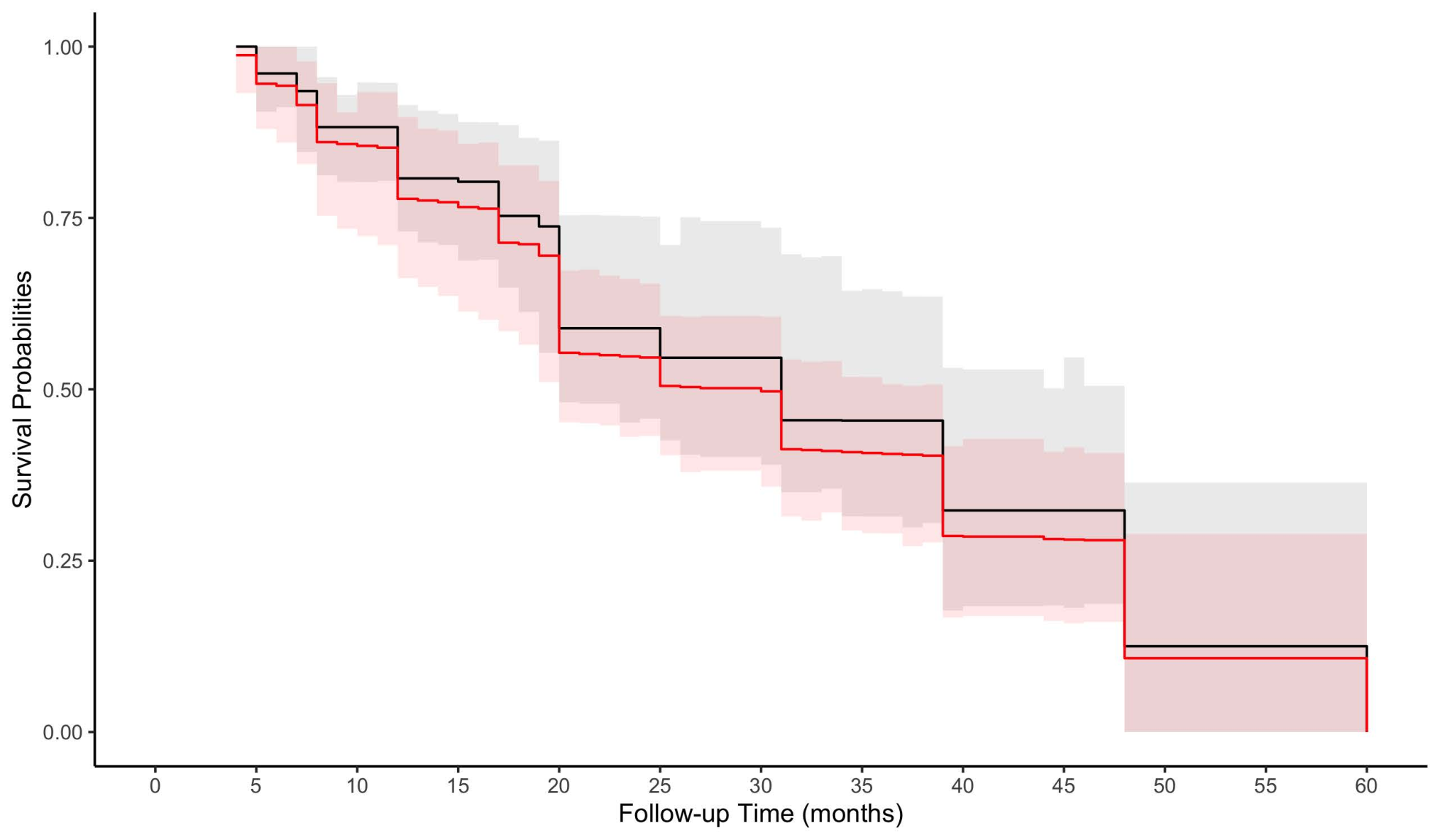
We set X=1X=1 if a patient had received adjuvant chemotherapy following the initial radiation treatment and 0 otherwise. Hence, XX is a time independent covariate, and we fit the model h⁡(t|X)=λ⁡(t)+X​βh(t|X)=\lambda(t)+X\beta to the data using the proposed method. Here, β\beta represents the difference in the hazard of breast retraction between X=1X=1 and X=0X=0 groups at any time point. We obtain β^=0.031\widehat{\beta}=0.031. Since the choice of hnh_{n} was quite arbitrary in the profile likelihood-based method of standard error, we used different values of hnh_{n}, 1.5n−1/21.5n^{-1/2}, n−1/2/20n^{-1/2}/20, n−1/2/100n^{-1/2}/100 and n−1/2/1000n^{-1/2}/1000, and obtained 0.090.09, 0.080.08, 0.060.06 and 0.0070.007 as the standard errors. Obviously, for standard error 0.0070.007, β^\widehat{\beta} is significantly different from zero at the 5%5\% level, while for other standard errors β^\widehat{\beta} is not significantly different from zero. To investigate this issue further, we calculated bootstrap standard errors using 200200 bootstrap samples, which came out to be 0.06. Figure 1 plots the estimated survival curves for the two groups along with their 95% pointwise confidence intervals calculated using the bootstrap method. This analysis shows no significant difference between the two survival functions or the two hazards functions at any time. On the contrary, Finkelstein 1986 fit a proportional hazard model to this data and found a statistically significant effect of chemotherapy.

[Figure 1 should be here]

6 Implementation: R package MMIntAdd

For the implementation of our proposed method, we have developed an R package, and it is available at GitHub: https://github.com/laozaoer/MMIntAdd. In this section, we discuss how the package can be used to analyze the breast cosmesis dataset. The first step is installing the package. One can use the R package devtools to install our R package as follows.

>library(devtools)
>devtools::install_github("laozaoer/MMIntAdd")

If the above method fails, then alternatively one may use the remotes package to install MMIntAdd. The code is

>library(remotes)
>remotes::install_github("laozaoer/MMIntAdd")

During the installation, when asked, it is customary to update the dependent packages, Rcpp, RcppArmadillo, or boot. After installation, load the package in the R console using the command

>library(MMIntAdd)

Let us now analyze the breast cosmesis data available in the package. This dataset was taken from the interval package and reformatted. Unlike the description given in Section 2, the first two columns of the dataset do not represent the finite inspection time window; rather, they represent the two boundary points of the time-to-event. Specifically, for a left-censored subject, the entry in the first column is zero, while the entry of the second column is infinity for a right-censored subject. The following three columns are left-, interval-, and right-censoring indicators. Note that the sum of these indicators must be equal to one for any subject. The sixth column of the data represents the covariate value.

> data(bcos)
> head(bcos)
left right L I R covariate
1 45 Inf 0 0 1 0
2 6 10 0 1 0 0
3 0 7 1 0 0 0
4 46 Inf 0 0 1 0
5 46 Inf 0 0 1 0
6 7 16 0 1 0 0

There are two functions of the MMIntAdd package, Add_case2_inte and Add_ci_boot. To find them, use the command

> lsf.str("package:MMIntAdd")
Add_case2_inte : function (data, hn.m, Max_iter = 1000, Tol = 0.001)
Add_ci_boot : function (data, time_points, covariate_value, CItype =
c("norm", "basic","perc", "bca"), conf = 0.95, boot.num = 200,
object_type =c("reg"), Max_iter = 1000, Tol = 0.001)

The first function returns the regression parameter estimates and the standard error calculated using the profile likelihood approach. For the standard error calculation, we require the bandwidth that is given as an input argument, hn.m of the function. Different values of hn.m returns different standard errors but with the same parameter estimates.

> result_hn1=Add_case2_inte(bcos,hn.m=1.5)
> print(result_hn1$beta)
Est SE
[1,] 0.03136608 0.09057521
> result_hn2=Add_case2_inte(bcos,hn.m=1/20)
> print(result_hn2$beta)
Est SE
[1,] 0.03136608 0.08259436
> result_hn3=Add_case2_inte(bcos,hn.m=1/100)
> print(result_hn3$beta)
Est SE
[1,] 0.03136608 0.05657365
> result_hn4=Add_case2_inte(bcos,hn.m=1/1000)
> print(result_hn4$beta)
Est SE
[1,] 0.03136608 0.007612

The other returned objects of Add_case2_inte are the estimates of λ=(λ1,…,λm)⊤\lambda=(\lambda_{1},\ldots,\lambda_{m})^{\top}, the log-likelihood value and the set of distinct inspection time points.

The other function of the MMIntAdd package is used to obtain the bootstrap standard error and confidence interval. There are many input arguments to that function. Among them, boot.num denotes the number of bootstrap samples to be used.

> Add_ci_boot(bcos,boot.num = 200)
$beta_boot_se
Est boot_se
covariate 0.03136608 0.06354992
$CI_beta
$CI_beta$normal
index method lwr upr
normal 1 normal -0.1092515 0.1398596
$CI_beta$basic
index method lwr upr
basic 1 basic -0.1277781 0.06273215
$CI_beta$percent
index method lwr upr
percent 1 percent 3.127308e-55 0.1905102
$CI_beta$bca
index method lwr upr
bca 1 bca 3.142232e-37 0.240083

The above function returns bootstrap standard error and bootstrap confidence intervals of the regression parameter, which varies according to the method chosen. Although the default confidence level is 0.95, the level can be set to a different value. These functions can also handle multiple covariates. All the covariates must be binary or numeric, and they are placed from the sixth column onwards in the data frame. For analyzing data with a categorical covariate with kk nominal categories, the (k−1)(k-1) dummy variables must be incorporated in the data frame.

Next, we analyze a simulated dataset using the MMIntAdd package.

> set.seed(10)
> n=100
> # Generation of three covariates
> x1=rbinom(n, 1, 0.5) # the first covariate
> x2=rbinom(n, 1, 0.4) # the second covariate
> x3=rbinom(n, 1, 0.3) # the third covariate
>
> #caplambda=0.2*t+ t*(0.5*x1+1*x2+0.6*x3), the true value of the
> #regression parameters are 0.5, 1 and 0.6.
> r=runif(n, 0, 1)
> time_to_event=-log(r)/(0.2+ 0.5*x1+1*x2+0.6*x3)
> # Generation of inspection time window (L, R)
> myl= runif(n,0.1,1.5)
> myr=runif(n, myl+1.5, 4)
> #### Censoring indicator
> delta_ell=as.numeric(time_to_event<myl)
> delta_r=as.numeric(time_to_event>myr)
> delta_i=1-delta_ell-delta_r
>
> myr[delta_ell==1]=myl[delta_ell==1]
> myl[delta_ell==1]=0
> myl[delta_r==1]=myr[delta_r==1]
> myr[delta_r==1]=Inf
> # Creation of the final data object
> mydata=data.frame(myl, myr, delta_ell, delta_i, delta_r, x1,x2,x3)
> mydata=as.matrix(mydata)
> # Analysis of the data by invoking the following function
> testresult=Add_case2_inte(mydata,hn.m=1.5)
> testresult$beta
Est SE
x1 0.7008246 0.2899771
x2 1.0521943 0.3808892
x3 0.4904499 0.2564767

Suppose that, for this example, we are interested in obtaining the bootstrap standard error of the regression parameters and the bootstrap confidence interval of the survival probability at select time points and for a given set of covariate values. For illustration, suppose that the interest is in the survival probability at only two time points, 0.5 and 0.6, and for a covariate value of (0, 1, 0). The code is

> mytimepoints=c(0.5, 0.6)
> mycov=c(0, 1, 0)
> out=Add_ci_boot(mydata,time_points=mytimepoints,
+ covariate_value = mycov, object_type = c("reg","surv"))
> names(out)
[1] "beta_boot_se" "CI_beta" "surv_boot_se" "CI_surv"
> out$beta_boot_se
Est boot_se
x1 0.7008246 0.2365580
x2 1.0521943 0.3334506
x3 0.4904499 0.2776679
> out$CI_beta
$normal
index method lwr upr
normal 1 normal 0.29612686 1.223417
normal1 2 normal 0.37157108 1.678673
normal2 3 normal -0.04340368 1.045034
$basic
index method lwr upr
basic 1 basic 0.2265320 1.248173
basic1 2 basic 0.2608937 1.607011
basic2 3 basic -0.1692522 0.980646
$percent
index method lwr upr
percent 1 percent 0.1534763545 1.175117
percent1 2 percent 0.4973772979 1.843495
percent2 3 percent 0.0002538463 1.150152
$bca
index method lwr upr
bca 1 bca 0.406808700 1.703756
bca1 2 bca 0.478899213 1.833237
bca2 3 bca 0.001413554 1.175776
> out$surv_boot_se
Est boot_se
1 0.4096685 0.1283081
2 0.2226586 0.1198392
> out$CI_surv
$normal
index method lwr upr
normal 1 normal 0.23085708 1.0000000
normal1 2 normal 0.07454217 0.5108168
$basic
index method lwr upr
basic 1 basic 0.27802103 1.0000000
basic1 2 basic 0.08806235 0.6798638
$percent
index method lwr upr
percent 1 percent 0.11100018 0.6036531
percent1 2 percent 0.07292174 0.5629745
$bca
index method lwr upr
bca 1 bca 0.23570171 0.6307615
bca1 2 bca 0.02607938 0.4095530

After examining all the results, we recommend using the BCA confidence interval (Efron and Tibshirani 1993) for the regression parameters and the survival probabilities.

7 Conclusions

This chapter proposed an efficient MM algorithm to obtain ML estimates of a complex likelihood function for the ARM with interval-censored responses. The attractive feature of the method is enabling the separation of the finite and infinite dimensional parameters. This separation of components provides significant computational advantages as the dimension of the infinite-dimensional parameter increases with the sample size. Numerical studies show that the algorithm works well; we have not encountered any convergence issues in the simulation settings or real data analysis.

We believe that this MM proposal will help generate new ideas for handling computational bottlenecks in complex models and likelihoods. Model (1) assumes a constant effect of the covariate. However, rather than a constant regression parameter, one can consider a time-dependent coefficient β⁡(t)\beta(t) without specifying any form (Huffer and McKeague 1991). Some other interesting topics for future research include developing MM-based computationally efficient methods and algorithms for the clustered case-I or case-II interval-censored responses (Huang 1996; Wang et al. 2022), including exploration of big-data scalability in tune to recent advances via asynchronous distributed EM algorithms (Srivastava et al. 2019). Additionally, developing computationally efficient methods when the inspection time is informative (Zhao et al. 2021) could also be a direction of future research.

Acknowledgement

Bandyopadhyay acknowledges funding support from the NIH/NCI grants P20CA252717, P20CA264067, and P30CA016059 (VCU’s Massey Cancer Center Support Grant).

References

  • Bogaerts et al. (2018) Bogaerts, K., Koma´\acute{\rm a}rek, A., and Lesaffre, E. (2018). Survival Analysis with Interval-Censored Data: A Practical Approach with Examples in R, SAS, and BUGS. CRC/Taylor & Francis Group.
  • Efron and Tibshirani (1993) Efron, B. and Tibshirani, R. J. (1993). An Introduction to the Bootstrap. Chapman and Hall: New York, NY.
  • Finkelstein (1986) Finkelstein, D. M. (1986). A proportional hazards model for interval-censored failure time data. Biometrics 42, 845–854.
  • Finkelstein and Wolfe (1985) Finkelstein, D. M. and Wolfe, R. A. (1985). A semiparametric model for regression analysis of interval-censored failure time data. Biometrics 41, 933–945.
  • Fletcher (2013) Fletcher, R. (2013). Practical Methods of Optimization. John Wiley & Sons.
  • Huang (1996) Huang, J. (1996). Efficient estimation for the proportional hazards model with interval censoring. Annals of Statistics 24, 540–568.
  • Huang et al. (2019) Huang, X., Xu, J., and Tian, G. (2019). On profile MM algorithms for Gamma frailty survival models. Statistica Sinica 29, 895–916.
  • Huffer and McKeague (1991) Huffer, F. W. and McKeague, I. W. (1991). Weighted least squares estimation for Aalen’s additive risk model. Journal of the American Statistical Association 86, 114–129.
  • Hunter and Lange (2000) Hunter, D. R. and Lange, K. (2000). Quantile regression via an MM algorithm. Journal of Computational and Graphical Statistics 9, 60–77.
  • Hunter and Lange (2002) Hunter, D. R. and Lange, K. (2002). Computing estimates in the proportional odds model. Annals of the Institute of Statistical Mathematics 54, 155–168.
  • Hunter and Lange (2004) Hunter, D. R. and Lange, K. (2004). A tutorial on MM algorithms. The American Statistician 58, 30–37.
  • Hunter and Li (2005) Hunter, D. R. and Li, R. (2005). Variable selection using MM algorithms. Annals of Statistics 33, 1617–1642.
  • Lin and Ying (1994a) Lin, D. and Ying, Z. (1994a). Semiparametric analysis of the additive risk model. Biometrika 81, 61–71.
  • Lin and Ying (1994b) Lin, D. Y. and Ying, Z. (1994b). Semiparametric analysis of the additive risk model. Biometrika 81, 61–71.
  • Martinussen and Scheike (2002) Martinussen, T. and Scheike, T. H. (2002). Efficient estimation in additive hazards regression with current status data. Biometrika 89, 649–658.
  • Murphy and Van der Vaart (2000) Murphy, S. A. and Van der Vaart, A. W. (2000). On profile likelihood. Journal of the American Statistical Association 95, 449–465.
  • Nguyen (2017) Nguyen, H. D. (2017). An introduction to MM algorithms for machine learning and statistical estimation. WIREs Data Mining and Knowledge Discovery page 7(e1198).
  • Srivastava et al. (2019) Srivastava, S., DePalma, G., and Liu, C. (2019). An asynchronous distributed expectation maximization algorithm for massive data: the DEM algorithm. Journal of Computational and Graphical Statistics 28, 233–243.
  • Wang et al. (2010) Wang, L., Sun, J., and Tong, X. (2010). Regression analysis of case-II interval-censored failure time data with the additive hazards model. Statistica Sinica 20, 1709–1723.
  • Wang et al. (2020) Wang, P., Zhou, Y., and Sun, J. (2020). A new method for regression analysis of interval-censored data with the additive hazards model. Journal of the Korean Statistical Society 49, 1131–1147.
  • Wang et al. (2022) Wang, T., He, K., Ma, W., Bandyopadhyay, D., and Sinha, S. (2022). Minorize-maximize algorithm for the generalized odds rate model for clustered current status data. To appear in the Canadian Journal of Statistics .
  • Wu and Lange (2010) Wu, T. T. and Lange, K. (2010). The MM alternative to EM. Statistical Science 25, 492–505.
  • Zeng et al. (2006) Zeng, D., Cai, J., and Shen, Y. (2006). Semiparametric additive risks model for interval-censored data. Statistica Sinica 16, 287–302.
  • Zhang and Sun (2010) Zhang, Z. and Sun, J. (2010). Interval censoring. Statistical Methods in Medical Research 19, 53–70.
  • Zhao et al. (2021) Zhao, B., Wang, S., Wang, C., and Sun, J. (2021). New methods for the additive hazards model with the informatively interval-censored failure time data. Biometrical Journal 63, 1507–1525.
  • Zhou and Zhang (2012) Zhou, H. and Zhang, Y. (2012). EM vs MM: A case study. Computational Statistics & Data Analysis 56, 3909–3920.

Appendix

We shall use the second part of Lemma 1 from Wang et al. 2022 in proving Theorem 1, and we present this result in the following proposition. The proof of proposition 1 can be found in Wang et al. 2022.

Proposition 1

(Wang et al. 2022) For any τ,τ0≥0\tau,\tau_{0}\geq 0

log⁡{1−exp⁡(−τ)1−exp⁡(−τ0)}≥(τ−τ0)​A1​(τ0)−(τ−τ0)2​A2​(τ0)+log⁡(τ0τ)+1−τ0τ,\displaystyle{\rm log}\left\{\frac{1-\exp(-\tau)}{1-\exp(-\tau_{0})}\right\}\geq(\tau-\tau_{0})A_{1}(\tau_{0})-(\tau-\tau_{0})^{2}A_{2}(\tau_{0})+{\rm log}\left(\frac{\tau_{0}}{\tau}\right)+1-\frac{\tau_{0}}{\tau},

where A1​(τ0)=exp⁡(−τ0)/{1−exp⁡(−τ0)}A_{1}(\tau_{0})=\exp(-\tau_{0})/\{1-\exp(-\tau_{0})\} and A2​(τ0)=exp⁡(−τ0)/2​{1−exp⁡(−τ0)}2A_{2}(\tau_{0})=\exp(-\tau_{0})/2\{1-\exp(-\tau_{0})\}^{2}.

A.1 Proof of Theorem 1

In ℓ2​(λ,β)\ell_{2}(\lambda,\beta) and ℓ4​(λ,β)\ell_{4}(\lambda,\beta), (λ1,…,λm)⊤(\lambda_{1},\ldots,\lambda_{m})^{\top} are not entangled with β\beta. Therefore, there is no need to develop the minorization functions for them. In the following, we show how to find the minorization functions for ℓ1​(λ,β)\ell_{1}(\lambda,\beta) and ℓ3​(λ,β)\ell_{3}(\lambda,\beta). Define u(Li,Xi)=∑k:tk≤Liλk+β⊤Zxi(Li)u(L_{i},X_{i})=\sum_{k:t_{k}\leq L_{i}}\lambda_{k}+\beta^{\top}Z_{x_{i}}(L_{i}), u(Ri,Xi)=∑k:tk≤Riλk+β⊤Zxi(Ri)u(R_{i},X_{i})=\sum_{k:t_{k}\leq R_{i}}\lambda_{k}+\beta^{\top}Z_{x_{i}}(R_{i}) and u(Li,Ri,Xi)=∑k:Li<tk≤Riλk+β⊤{Zxi(Ri)−Zxi(Li)}u(L_{i},R_{i},X_{i})=\sum_{k:L_{i}<t_{k}\leq R_{i}}\lambda_{k}+\beta^{\top}\{Z_{x_{i}}(R_{i})-Z_{x_{i}}(L_{i})\}. According to our model assumption (1), u⁡(Li,Xi)>0u(L_{i},X_{i})>0, u⁡(Ri,Xi)>0u(R_{i},X_{i})>0 and u⁡(Li,Ri,Xi)>0u(L_{i},R_{i},X_{i})>0 for all ii. Now, we can re-write

ℓ1​(λ,β)\displaystyle\ell_{1}(\lambda,\beta) =\displaystyle= ∑i=1nΔL,ilog[1−exp{−∑k:tk≤Liλk−β⊤Zxi(Li)}]\displaystyle\sum_{i=1}^{n}\Delta_{L,i}{\rm log}[1-\exp\{-\sum_{k:t_{k}\leq L_{i}}\lambda_{k}-\beta^{\top}Z_{x_{i}}(L_{i})\}]
=\displaystyle= ∑i=1nΔL,i​log​[1−exp⁡{−u⁡(Li,Xi)}]\displaystyle\sum_{i=1}^{n}\Delta_{L,i}{\rm log}[1-\exp\{-u(L_{i},X_{i})\}]
=\displaystyle= ∑i=1nΔL,i​(log⁡[1−exp⁡{−u0​(Li,Xi)}]+log⁡[1−exp⁡{−u⁡(Li,Xi)}1−exp⁡{−u0​(Li,Xi)}]).\displaystyle\sum_{i=1}^{n}\Delta_{L,i}\left({\rm log}[1-\exp\{-u_{0}(L_{i},X_{i})\}]+{\rm log}\left[\frac{1-\exp\{-u(L_{i},X_{i})\}}{1-\exp\{-u_{0}(L_{i},X_{i})\}}\right]\right).

Applying proposition 1 to the second term of the above display with τ=u⁡(Li,Xi)\tau=u(L_{i},X_{i}) and τ0=u0​(Li,Xi)\tau_{0}=u_{0}(L_{i},X_{i}), we obtain

ℓ1​(λ,β)\displaystyle\ell_{1}(\lambda,\beta) ≥\displaystyle\geq ∑i=1nΔL,i​(log⁡[1−exp⁡{−u0​(Li,Xi)}]+{u⁡(Li,Xi)−u0​(Li,Xi)}​A1​(u0​(Li,Xi))CLOSE\displaystyle\sum_{i=1}^{n}\Delta_{L,i}\biggl({\rm log}[1-\exp\{-u_{0}(L_{i},X_{i})\}]+\{u(L_{i},X_{i})-u_{0}(L_{i},X_{i})\}A_{1}(u_{0}(L_{i},X_{i})) (A.1)
−{u(Li,Xi)−u0(Li,Xi)}2A2(u0(Li,Xi))+log{u0​(Li,Xi)u⁡(Li,Xi)}+1−u0​(Li,Xi)u⁡(Li,Xi))\displaystyle-\{u(L_{i},X_{i})-u_{0}(L_{i},X_{i})\}^{2}A_{2}(u_{0}(L_{i},X_{i}))+{\rm log}\left\{\frac{u_{0}(L_{i},X_{i})}{u(L_{i},X_{i})}\right\}+1-\frac{u_{0}(L_{i},X_{i})}{u(L_{i},X_{i})}\biggl)
=\displaystyle= ∑i=1nΔL,i[{A1(u0(Li,Xi))+2A2(u0(Li,Xi))u0(Li,Xi)}u(Li,Xi)−A2(u0(Li,Xi))u2(Li,Xi)\displaystyle\sum_{i=1}^{n}\Delta_{L,i}\Bigg[\{A_{1}(u_{0}(L_{i},X_{i}))+2A_{2}(u_{0}(L_{i},X_{i}))u_{0}(L_{i},X_{i})\}u(L_{i},X_{i})-A_{2}(u_{0}(L_{i},X_{i}))u^{2}(L_{i},X_{i})
+log{u0​(Li,Xi)u⁡(Li,Xi)}−u0​(Li,Xi)u⁡(Li,Xi)+C1(u0(Li,Xi))]\displaystyle+{\rm log}\left\{\frac{u_{0}(L_{i},X_{i})}{u(L_{i},X_{i})}\right\}-\frac{u_{0}(L_{i},X_{i})}{u(L_{i},X_{i})}+C_{1}(u_{0}(L_{i},X_{i}))\Bigg]
=\displaystyle= ∑i=1nΔL,i[{A1(u0(Li,Xi))+2A2(u0(Li,Xi))u0(Li,Xi)}(∑k:tk≤Liλk+β⊤Zxi(Li))\displaystyle\sum_{i=1}^{n}\Delta_{L,i}\Bigg[\{A_{1}(u_{0}(L_{i},X_{i}))+2A_{2}(u_{0}(L_{i},X_{i}))u_{0}(L_{i},X_{i})\}\left(\sum_{k:t_{k}\leq L_{i}}\lambda_{k}+\beta^{\top}Z_{x_{i}}(L_{i})\right)
−A2(u0(Li,Xi))(∑k:tk≤Liλk+β⊤Zxi(Li))2+log(u0​(Li,Xi)∑k:tk≤Liλk+β⊤Zxi(Li))\displaystyle-A_{2}(u_{0}(L_{i},X_{i}))\left(\sum_{k:t_{k}\leq L_{i}}\lambda_{k}+\beta^{\top}Z_{x_{i}}(L_{i})\right)^{2}+{\rm log}\left(\frac{u_{0}(L_{i},X_{i})}{\sum_{k:t_{k}\leq L_{i}}\lambda_{k}+\beta^{\top}Z_{x_{i}}(L_{i})}\right)
−(u0​(Li,Xi)∑k:tk≤Liλk+β⊤Zxi(Li))+C1(u0(Li,Xi))],\displaystyle-\left(\frac{u_{0}(L_{i},X_{i})}{\sum_{k:t_{k}\leq L_{i}}\lambda_{k}+\beta^{\top}Z_{x_{i}}(L_{i})}\right)+C_{1}(u_{0}(L_{i},X_{i}))\Bigg],

where C1​(u0​(Li,Xi))C_{1}(u_{0}(L_{i},X_{i})) is the constant term that only depends on u0​(Li,Xi)u_{0}(L_{i},X_{i}), given as C1​(u0​(Li,Xi))=log⁡[1−exp⁡{−u0​(Li,Xi)}]−A1​(u0​(Li,Xi))​u0​(Li,Xi)−A2​(u0​(Li,Xi))​u02​(Li,Xi)+1.C_{1}(u_{0}(L_{i},X_{i}))={\rm log}[1-\exp\{-u_{0}(L_{i},X_{i})\}]-A_{1}(u_{0}(L_{i},X_{i}))u_{0}(L_{i},X_{i})-A_{2}(u_{0}(L_{i},X_{i}))u_{0}^{2}(L_{i},X_{i})+1. Next, we look into the following three terms of (A.1). First,

−(∑tk≤Liλk+β⊤​Zxi​(Li))2\displaystyle-\left(\sum_{t_{k}\leq L_{i}}\lambda_{k}+\beta^{\top}Z_{x_{i}}(L_{i})\right)^{2} =\displaystyle= −(∑tk≤Liλk​0u0​(Li,Xi)​u0​(Li,Xi)λk​0​λk+β0⊤​Zxi​(Li)u0​(Li,Xi)​u0​(Li,Xi)β0⊤​Zxi​(Li)​β⊤​Zxi​(Li))2\displaystyle-\left(\sum_{t_{k}\leq L_{i}}\frac{\lambda_{k0}}{u_{0}(L_{i},X_{i})}\frac{u_{0}(L_{i},X_{i})}{\lambda_{k0}}\lambda_{k}+\frac{\beta_{0}^{\top}Z_{x_{i}}(L_{i})}{u_{0}(L_{i},X_{i})}\frac{u_{0}(L_{i},X_{i})}{\beta_{0}^{\top}Z_{x_{i}}(L_{i})}\beta^{\top}Z_{x_{i}}(L_{i})\right)^{2}
≥\displaystyle\geq −{∑tk≤Liu0​(Li,Xi)λk​0λk2+u0​(Li,Xi)β0⊤​Zxi​(Li)(β⊤Zxi(Li))2},\displaystyle-\biggl\{\sum_{t_{k}\leq L_{i}}\frac{u_{0}(L_{i},X_{i})}{\lambda_{k0}}\lambda_{k}^{2}+\frac{u_{0}(L_{i},X_{i})}{\beta_{0}^{\top}Z_{x_{i}}(L_{i})}(\beta^{\top}Z_{x_{i}}(L_{i}))^{2}\biggl\},

where, the inequality is obtained by applying Jensen’s inequality on the concave function f⁡(x)=−x2f(x)=-x^{2} and noting that ∑k:tk≤Liλk​0/u0(Li,Xi)+β0⊤Zxi(Li)/u0(Li,Xi)=1\sum_{k:t_{k}\leq L_{i}}\lambda_{k0}/u_{0}(L_{i},X_{i})+\beta_{0}^{\top}Z_{x_{i}}(L_{i})/u_{0}(L_{i},X_{i})=1. Second, applying the standard inequality log⁡(x)≥1−1/x{\rm log}(x)\geq 1-1/x for any generic x>0x>0, we have

log⁡(u0​(Li,Xi)∑tk≤Liλk+β⊤​Zxi​(Li))≥1−∑tk≤Liλk+β⊤​Zxi​(Li)u0​(Li,Xi),\displaystyle{\rm log}\left(\frac{u_{0}(L_{i},X_{i})}{\sum_{t_{k}\leq L_{i}}\lambda_{k}+\beta^{\top}Z_{x_{i}}(L_{i})}\right)\geq 1-\frac{\sum_{t_{k}\leq L_{i}}\lambda_{k}+\beta^{\top}Z_{x_{i}}(L_{i})}{u_{0}(L_{i},X_{i})},

and third,

−u0​(Li,Xi)∑tk≤Liλk+β⊤​Zxi​(Li)\displaystyle-\frac{u_{0}(L_{i},X_{i})}{\sum_{t_{k}\leq L_{i}}\lambda_{k}+\beta^{\top}Z_{x_{i}}(L_{i})} =\displaystyle= −u0(Li,Xi){∑tk≤Liλk​0u0​(Li,Xi)u0​(Li,Xi)λk​0λk\displaystyle-u_{0}(L_{i},X_{i})\biggl\{\sum_{t_{k}\leq L_{i}}\frac{\lambda_{k0}}{u_{0}(L_{i},X_{i})}\frac{u_{0}(L_{i},X_{i})}{\lambda_{k0}}\lambda_{k}
+β0⊤​Zxi​(Li)u0​(Li,Xi)u0​(Li,Xi)β0⊤​Zxi​(Li)β⊤Zxi(Li)}−1\displaystyle+\frac{\beta_{0}^{\top}Z_{x_{i}}(L_{i})}{u_{0}(L_{i},X_{i})}\frac{u_{0}(L_{i},X_{i})}{\beta_{0}^{\top}Z_{x_{i}}(L_{i})}\beta^{\top}Z_{x_{i}}(L_{i})\biggl\}^{-1}
≥\displaystyle\geq −[∑tk≤Liλk​02u0​(Li,Xi)λk−1+{β0⊤​Zxi​(Li)}2u0​(Li,Xi){β⊤Zxi(Li)}−1],\displaystyle-\biggl[\sum_{t_{k}\leq L_{i}}\frac{\lambda_{k0}^{2}}{u_{0}(L_{i},X_{i})}\lambda_{k}^{-1}+\frac{\{\beta_{0}^{\top}Z_{x_{i}}(L_{i})\}^{2}}{u_{0}(L_{i},X_{i})}\{\beta^{\top}Z_{x_{i}}(L_{i})\}^{-1}\biggl],

where, the last inequality is obtained by applying Jensen’s inequality on the concave function f(x)=−1/xf(x)=-1/x, and noting that ∑k:tk≤Liλk​0/u0(Li,Xi)+β0⊤Zxi(Li)/u0(Li,Xi)=1\sum_{k:t_{k}\leq L_{i}}\lambda_{k0}/u_{0}(L_{i},X_{i})+\beta_{0}^{\top}Z_{x_{i}}(L_{i})/u_{0}(L_{i},X_{i})=1. Then, applying the last three inequalities in (A.1), we obtain ℓ1(λ,β)≥ℓ1,†(λ,β|λ0,β0)≡∑k=1mℳ1,1,k(λk|λ0,β0)+ℳ1,2(β|λ0,β0)+ℳ1,3(λ0,β0)\ell_{1}(\lambda,\beta)\geq\ell_{1,\dagger}(\lambda,\beta|\lambda_{0},\beta_{0})\equiv\sum_{k=1}^{m}\mathcal{M}_{1,1,k}(\lambda_{k}|\lambda_{0},\beta_{0})+\mathcal{M}_{1,2}(\beta|\lambda_{0},\beta_{0})+\mathcal{M}_{1,3}(\lambda_{0},\beta_{0}), where for k=1,…,mk=1,\dots,m,

ℳ1,1,k​(λk|λ0,β0)\displaystyle\mathcal{M}_{1,1,k}(\lambda_{k}|\lambda_{0},\beta_{0}) =\displaystyle= ∑i=1nΔL,i[{A1(u0(Li,Xi))+2A2(u0(Li,Xi))u0(Li,Xi)}λk\displaystyle\sum_{i=1}^{n}\Delta_{L,i}\Bigg[\{A_{1}(u_{0}(L_{i},X_{i}))+2A_{2}(u_{0}(L_{i},X_{i}))u_{0}(L_{i},X_{i})\}\lambda_{k}
−A2(u0(Li,Xi)){u0​(Li,Xi)λk​0}λk2−λku0​(Li,Xi)−λk​02u0​(Li,Xi)λk−1]I(tk≤Li),\displaystyle-A_{2}(u_{0}(L_{i},X_{i}))\left\{\frac{u_{0}(L_{i},X_{i})}{\lambda_{k0}}\right\}\lambda_{k}^{2}-\frac{\lambda_{k}}{u_{0}(L_{i},X_{i})}-\frac{\lambda_{k0}^{2}}{u_{0}(L_{i},X_{i})}\lambda_{k}^{-1}\Bigg]I(t_{k}\leq L_{i}),
ℳ1,2​(β|λ0,β0)\displaystyle\mathcal{M}_{1,2}(\beta|\lambda_{0},\beta_{0}) =\displaystyle= ∑i=1nΔL,i[{A1(u0(Li,Xi))+2A2(u0(Li,Xi))u0(Li,Xi)}β⊤Zxi(Li)\displaystyle\sum_{i=1}^{n}\Delta_{L,i}\Bigg[\{A_{1}(u_{0}(L_{i},X_{i}))+2A_{2}(u_{0}(L_{i},X_{i}))u_{0}(L_{i},X_{i})\}\beta^{\top}Z_{x_{i}}(L_{i})
−A2​(u0​(Li,Xi))​u0​(Li,Xi)β0⊤​Zxi​(Li)​{β⊤​Zxi​(Li)}2−β⊤​Zxi​(Li)u0​(Li,Xi)\displaystyle-A_{2}(u_{0}(L_{i},X_{i}))\frac{u_{0}(L_{i},X_{i})}{\beta_{0}^{\top}Z_{x_{i}}(L_{i})}\{\beta^{\top}Z_{x_{i}}(L_{i})\}^{2}-\frac{\beta^{\top}Z_{x_{i}}(L_{i})}{u_{0}(L_{i},X_{i})}
−{β0⊤​Zxi​(Li)}2u0​(Li,Xi){β⊤Zxi(Li)}−1],\displaystyle-\frac{\{\beta_{0}^{\top}Z_{x_{i}}(L_{i})\}^{2}}{u_{0}(L_{i},X_{i})}\{\beta^{\top}Z_{x_{i}}(L_{i})\}^{-1}\Bigg],

and ℳ1,3(λ0,β0)=∑i=1nΔL,i{log[1−exp{−u0(Li,Xi)}]−A1(u0(Li,Xi))u0(Li,Xi)−A2(u0(Li,Xi))\mathcal{M}_{1,3}(\lambda_{0},\beta_{0})=\sum_{i=1}^{n}\Delta_{L,i}\{{\rm log}[1-\exp\{-u_{0}(L_{i},X_{i})\}]-A_{1}(u_{0}(L_{i},X_{i}))u_{0}(L_{i},X_{i})-A_{2}(u_{0}(L_{i},X_{i})) u02(Li,Xi)+1}u_{0}^{2}(L_{i},X_{i})+1\}. Next, consider finding the minorization function for ℓ3​(λ,β)\ell_{3}(\lambda,\beta). Here, we use the same techniques as finding the minorization function for ℓ1​(λ,β)\ell_{1}(\lambda,\beta). Note,

ℓ3​(λ,β)\displaystyle\ell_{3}(\lambda,\beta) =\displaystyle= ∑i=1nΔI,ilog(1−exp[−∑k:Li<tk≤Riλk−β⊤{Zxi(Ri)−Zxi(Li)}])\displaystyle\sum_{i=1}^{n}\Delta_{I,i}{\rm log}\left(1-\exp\left[-\sum_{k:L_{i}<t_{k}\leq R_{i}}\lambda_{k}-\beta^{\top}\{Z_{x_{i}}(R_{i})-Z_{x_{i}}(L_{i})\}\right]\right)
=\displaystyle= ∑i=1nΔI,i​log​[1−exp⁡{−u⁡(Li,Ri,Xi)}]\displaystyle\sum_{i=1}^{n}\Delta_{I,i}{\rm log}[1-\exp\{-u(L_{i},R_{i},X_{i})\}]
=\displaystyle= ∑i=1nΔI,i​(log⁡[1−exp⁡{−u0​(Li,Ri,Xi)}]+log⁡[1−exp⁡{−u⁡(Li,Ri,Xi)}1−exp⁡{−u0​(Li,Ri,Xi)}]).\displaystyle\sum_{i=1}^{n}\Delta_{I,i}\left({\rm log}[1-\exp\{-u_{0}(L_{i},R_{i},X_{i})\}]+{\rm log}\left[\frac{1-\exp\{-u(L_{i},R_{i},X_{i})\}}{1-\exp\{-u_{0}(L_{i},R_{i},X_{i})\}}\right]\right).

Now applying proposition 1 to the second term of the above display with τ=u⁡(Li,Ri,Xi)\tau=u(L_{i},R_{i},X_{i}) and τ0=u0​(Li,Ri,Xi)\tau_{0}=u_{0}(L_{i},R_{i},X_{i}), we obtain

ℓ3​(λ,β)\displaystyle\ell_{3}(\lambda,\beta) ≥\displaystyle\geq ∑i=1nΔI,i​(log⁡[1−exp⁡{−u0​(Li,Ri​Xi)}]+{u⁡(Li,Ri,Xi)−u0​(Li,Ri,Xi)}​A1​(u0​(Li,Ri,Xi))CLOSE\displaystyle\sum_{i=1}^{n}\Delta_{I,i}\biggl({\rm log}[1-\exp\{-u_{0}(L_{i},R_{i}X_{i})\}]+\{u(L_{i},R_{i},X_{i})-u_{0}(L_{i},R_{i},X_{i})\}A_{1}(u_{0}(L_{i},R_{i},X_{i})) (A.2)
−{u⁡(Li,Ri,Xi)−u0​(Li,Ri,Xi)}2​A2​(u0​(Li,Ri,Xi))\displaystyle-\{u(L_{i},R_{i},X_{i})-u_{0}(L_{i},R_{i},X_{i})\}^{2}A_{2}(u_{0}(L_{i},R_{i},X_{i}))
+log{u0​(Li,Ri,Xi)u⁡(Li,Ri,Xi)}+1−u0​(Li,Ri,Xi)u⁡(Li,Ri,Xi))\displaystyle+{\rm log}\left\{\frac{u_{0}(L_{i},R_{i},X_{i})}{u(L_{i},R_{i},X_{i})}\right\}+1-\frac{u_{0}(L_{i},R_{i},X_{i})}{u(L_{i},R_{i},X_{i})}\biggl)
=\displaystyle= ∑i=1nΔI,i[{A1(u0(Li,Ri,Xi))+2A2(u0(Li,Ri,Xi))u0(Li,Ri,Xi)}u(Li,Ri,Xi)\displaystyle\sum_{i=1}^{n}\Delta_{I,i}\Bigg[\{A_{1}(u_{0}(L_{i},R_{i},X_{i}))+2A_{2}(u_{0}(L_{i},R_{i},X_{i}))u_{0}(L_{i},R_{i},X_{i})\}u(L_{i},R_{i},X_{i})
−A2​(u0​(Li,Ri,Xi))​u2​(Li,Ri,Xi)\displaystyle-A_{2}(u_{0}(L_{i},R_{i},X_{i}))u^{2}(L_{i},R_{i},X_{i})
+log{u0​(Li,Ri,Xi)u⁡(Li,Ri,Xi)}−u0​(Li,Ri,Xi)u⁡(Li,Ri,Xi)+C1(u0(Li,Ri,Xi))]\displaystyle+{\rm log}\left\{\frac{u_{0}(L_{i},R_{i},X_{i})}{u(L_{i},R_{i},X_{i})}\right\}-\frac{u_{0}(L_{i},R_{i},X_{i})}{u(L_{i},R_{i},X_{i})}+C_{1}(u_{0}(L_{i},R_{i},X_{i}))\Bigg]
=\displaystyle= ∑i=1nΔI,i[{A1(u0(Li,Ri,Xi))\displaystyle\sum_{i=1}^{n}\Delta_{I,i}\Bigg[\{A_{1}(u_{0}(L_{i},R_{i},X_{i}))
+2A2(u0(Li,Ri,Xi))u0(Li,Ri,Xi)}(∑k:Li<tk≤Riλk+β⊤(Zxi(Ri)−Zxi(Li)))\displaystyle+2A_{2}(u_{0}(L_{i},R_{i},X_{i}))u_{0}(L_{i},R_{i},X_{i})\}\left(\sum_{k:L_{i}<t_{k}\leq R_{i}}\lambda_{k}+\beta^{\top}(Z_{x_{i}}(R_{i})-Z_{x_{i}}(L_{i}))\right)
−A2(u0(Li,Ri,Xi))(∑k:Li<tk≤Riλk+β⊤(Zxi(Ri)−Zxi(Li)))2\displaystyle-A_{2}(u_{0}(L_{i},R_{i},X_{i}))\left(\sum_{k:L_{i}<t_{k}\leq R_{i}}\lambda_{k}+\beta^{\top}(Z_{x_{i}}(R_{i})-Z_{x_{i}}(L_{i}))\right)^{2}
+log(u0​(Li,Ri,Xi)∑k:Li<tk≤Riλk+β⊤(Zxi(Ri)−Zxi(Li)))\displaystyle+{\rm log}\left(\frac{u_{0}(L_{i},R_{i},X_{i})}{\sum_{k:L_{i}<t_{k}\leq R_{i}}\lambda_{k}+\beta^{\top}(Z_{x_{i}}(R_{i})-Z_{x_{i}}(L_{i}))}\right)
−(u0​(Li,Ri,Xi)∑k:Li<tk≤Riλk+β⊤(Zxi(Ri)−Zxi(Li)))+C1(u0(Li,Ri,Xi))]\displaystyle-\left(\frac{u_{0}(L_{i},R_{i},X_{i})}{\sum_{k:L_{i}<t_{k}\leq R_{i}}\lambda_{k}+\beta^{\top}(Z_{x_{i}}(R_{i})-Z_{x_{i}}(L_{i}))}\right)+C_{1}(u_{0}(L_{i},R_{i},X_{i}))\Bigg]

where, C1​(u0​(Li,Ri,Xi))C_{1}(u_{0}(L_{i},R_{i},X_{i})) is the constant term that only depends on u0​(Li,Ri,Xi)u_{0}(L_{i},R_{i},X_{i}), given by C1​(u0​(Li,Ri,Xi))=log⁡[1−exp⁡{−u0​(Li,Ri,Xi)}]−A1​(u0​(Li,Ri,Xi))​u0​(Li,Ri,Xi)−A2​(u0​(Li,Ri,Xi))​u02​(Li,Ri,Xi)+1.C_{1}(u_{0}(L_{i},R_{i},X_{i}))={\rm log}[1-\exp\{-u_{0}(L_{i},R_{i},X_{i})\}]-A_{1}(u_{0}(L_{i},R_{i},X_{i}))u_{0}(L_{i},R_{i},X_{i})-A_{2}(u_{0}(L_{i},R_{i},X_{i}))u_{0}^{2}(L_{i},R_{i},X_{i})+1. Similarly, we have the following three inequalities,

−\displaystyle- (∑Li<tk≤Riλk+β⊤​(Zxi​(Ri)−Zxi​(Li)))2\displaystyle\left(\sum_{L_{i}<t_{k}\leq R_{i}}\lambda_{k}+\beta^{\top}(Z_{x_{i}}(R_{i})-Z_{x_{i}}(L_{i}))\right)^{2}
=\displaystyle= −(∑Li<tk≤Riλk​0u0​(Li,Ri,Xi)​u0​(Li,Ri,Xi)λk​0​λkCLOSE\displaystyle-\left(\sum_{L_{i}<t_{k}\leq R_{i}}\frac{\lambda_{k0}}{u_{0}(L_{i},R_{i},X_{i})}\frac{u_{0}(L_{i},R_{i},X_{i})}{\lambda_{k0}}\lambda_{k}\right.
OPEN+β0⊤​(Zxi​(Ri)−Zxi​(Li))u0​(Li,Ri,Xi)​u0​(Li,Ri,Xi)β0⊤​(Zxi​(Ri)−Zxi​(Li))​β0⊤​(Zxi​(Ri)−Zxi​(Li)))2\displaystyle\left.+\frac{\beta_{0}^{\top}(Z_{x_{i}}(R_{i})-Z_{x_{i}}(L_{i}))}{u_{0}(L_{i},R_{i},X_{i})}\frac{u_{0}(L_{i},R_{i},X_{i})}{\beta_{0}^{\top}(Z_{x_{i}}(R_{i})-Z_{x_{i}}(L_{i}))}\beta_{0}^{\top}(Z_{x_{i}}(R_{i})-Z_{x_{i}}(L_{i}))\right)^{2}
≥\displaystyle\geq −{∑Li<tk≤Riu0​(Li,Ri,Xi)λk​0λk2+u0​(Li,Ri,Xi)β0⊤​(Zxi​(Ri)−Zxi​(Li))(β⊤(Zxi(Ri)−Zxi(Li)))2},\displaystyle-\biggl\{\sum_{L_{i}<t_{k}\leq R_{i}}\frac{u_{0}(L_{i},R_{i},X_{i})}{\lambda_{k0}}\lambda_{k}^{2}+\frac{u_{0}(L_{i},R_{i},X_{i})}{\beta_{0}^{\top}(Z_{x_{i}}(R_{i})-Z_{x_{i}}(L_{i}))}(\beta^{\top}(Z_{x_{i}}(R_{i})-Z_{x_{i}}(L_{i})))^{2}\biggl\},
log⁡(u0​(Li,Ri,Xi)∑Li<tk≤Riλk+β⊤​(Zxi​(Ri)−Zxi​(Li)))≥1−∑Li<tk≤Riλk+β⊤​(Zxi​(Ri)−Zxi​(Li))u0​(Li,Ri,Xi),\displaystyle{\rm log}\left(\frac{u_{0}(L_{i},R_{i},X_{i})}{\sum_{L_{i}<t_{k}\leq R_{i}}\lambda_{k}+\beta^{\top}(Z_{x_{i}}(R_{i})-Z_{x_{i}}(L_{i}))}\right)\geq 1-\frac{\sum_{L_{i}<t_{k}\leq R_{i}}\lambda_{k}+\beta^{\top}(Z_{x_{i}}(R_{i})-Z_{x_{i}}(L_{i}))}{u_{0}(L_{i},R_{i},X_{i})},

and

−\displaystyle- u0​(Li,Ri,Xi)∑Li<tk≤Riλk+β⊤​(Zxi​(Ri)−Zxi​(Li))\displaystyle\frac{u_{0}(L_{i},R_{i},X_{i})}{\sum_{L_{i}<t_{k}\leq R_{i}}\lambda_{k}+\beta^{\top}(Z_{x_{i}}(R_{i})-Z_{x_{i}}(L_{i}))}
=\displaystyle= −u0(Li,Ri,Xi){∑Li<tk≤Riλk​0u0​(Li,Ri,Xi)u0​(Li,Ri,Xi)λk​0λk\displaystyle-u_{0}(L_{i},R_{i},X_{i})\biggl\{\sum_{L_{i}<t_{k}\leq R_{i}}\frac{\lambda_{k0}}{u_{0}(L_{i},R_{i},X_{i})}\frac{u_{0}(L_{i},R_{i},X_{i})}{\lambda_{k0}}\lambda_{k}
+β0⊤​(Zxi​(Ri)−Zxi​(Li))u0​(Li,Ri,Xi)u0​(Li,Ri,Xi)β0⊤​(Zxi​(Ri)−Zxi​(Li))β⊤(Zxi(Ri)−Zxi(Li))}−1\displaystyle+\frac{\beta_{0}^{\top}(Z_{x_{i}}(R_{i})-Z_{x_{i}}(L_{i}))}{u_{0}(L_{i},R_{i},X_{i})}\frac{u_{0}(L_{i},R_{i},X_{i})}{\beta_{0}^{\top}(Z_{x_{i}}(R_{i})-Z_{x_{i}}(L_{i}))}\beta^{\top}(Z_{x_{i}}(R_{i})-Z_{x_{i}}(L_{i}))\biggl\}^{-1}
≥\displaystyle\geq −[∑Li<tk≤Riλk​02u0​(Li,Ri,Xi)λk−1+{β0⊤​(Zxi​(Ri)−Zxi​(Li))}2u0​(Li,Ri,Xi){β⊤(Zxi(Ri)−Zxi(Li))}−1],\displaystyle-\biggl[\sum_{L_{i}<t_{k}\leq R_{i}}\frac{\lambda_{k0}^{2}}{u_{0}(L_{i},R_{i},X_{i})}\lambda_{k}^{-1}+\frac{\{\beta_{0}^{\top}(Z_{x_{i}}(R_{i})-Z_{x_{i}}(L_{i}))\}^{2}}{u_{0}(L_{i},R_{i},X_{i})}\{\beta^{\top}(Z_{x_{i}}(R_{i})-Z_{x_{i}}(L_{i}))\}^{-1}\biggl],

where, the first and the third inequalities are obtained by applying Jensen’s inequality on the concave function f⁡(x)=−x2f(x)=-x^{2} and f(x)=−1/xf(x)=-1/x, respectively, and the second inequality is obtained by applying the standard inequality log⁡(x)≥1−1/x{\rm log}(x)\geq 1-1/x. Applying the above two inequalities in (A.2), we obtain ℓ3(λ,β)≥ℓ3,†(λ,β|λ0,β0)≡∑k=1mℳ3,1,k(λk|λ0,β0)+ℳ3,2(β|λ0,β0)+ℳ3,3(λ0,β0)\ell_{3}(\lambda,\beta)\geq\ell_{3,\dagger}(\lambda,\beta|\lambda_{0},\beta_{0})\equiv\sum_{k=1}^{m}\mathcal{M}_{3,1,k}(\lambda_{k}|\lambda_{0},\beta_{0})+\mathcal{M}_{3,2}(\beta|\lambda_{0},\beta_{0})+\mathcal{M}_{3,3}(\lambda_{0},\beta_{0}), where

ℳ3,1,k​(λk|λ0,β0)\displaystyle\mathcal{M}_{3,1,k}(\lambda_{k}|\lambda_{0},\beta_{0}) =\displaystyle= ∑i=1nΔI,i[{A1(u0(Li,Ri,Xi))+2A2(u0(Li,Ri,Xi))u0(Li,Ri,Xi)}λk\displaystyle\sum_{i=1}^{n}\Delta_{I,i}\Bigg[\{A_{1}(u_{0}(L_{i},R_{i},X_{i}))+2A_{2}(u_{0}(L_{i},R_{i},X_{i}))u_{0}(L_{i},R_{i},X_{i})\}\lambda_{k}
−A2​(u0​(Li,Ri,Xi))​{u0​(Li,Ri,Xi)λk​0}​λk2\displaystyle-A_{2}(u_{0}(L_{i},R_{i},X_{i}))\left\{\frac{u_{0}(L_{i},R_{i},X_{i})}{\lambda_{k0}}\right\}\lambda_{k}^{2}
−λku0​(Li,Ri,Xi)−λk​02u0​(Li,Ri,Xi)λk−1]I(Li<tk≤Ri),k=1,…,m,\displaystyle-\frac{\lambda_{k}}{u_{0}(L_{i},R_{i},X_{i})}-\frac{\lambda_{k0}^{2}}{u_{0}(L_{i},R_{i},X_{i})}\lambda_{k}^{-1}\Bigg]I(L_{i}<t_{k}\leq R_{i}),\quad k=1,\ldots,m,
ℳ3,2​(β|λ0,β0)\displaystyle\mathcal{M}_{3,2}(\beta|\lambda_{0},\beta_{0}) =\displaystyle= ∑i=1nΔI,i​({A1​(u0​(Li,Ri,Xi))+2​A2​(u0​(Li,Ri,Xi))​u0​(Li,Ri,Xi)}CLOSE\displaystyle\sum_{i=1}^{n}\Delta_{I,i}\Bigg(\{A_{1}(u_{0}(L_{i},R_{i},X_{i}))+2A_{2}(u_{0}(L_{i},R_{i},X_{i}))u_{0}(L_{i},R_{i},X_{i})\}
×β⊤​{Zxi​(Ri)−Zxi​(Li)}−A2​(u0​(Li,Ri,Xi))​u0​(Li,Ri,Xi)​[β⊤​{Zxi​(Ri)−Zxi​(Li)}]2β0⊤​{Zxi​(Ri)−Zxi​(Li)}\displaystyle\times\beta^{\top}\{Z_{x_{i}}(R_{i})-Z_{x_{i}}(L_{i})\}-A_{2}(u_{0}(L_{i},R_{i},X_{i}))\frac{u_{0}(L_{i},R_{i},X_{i})[\beta^{\top}\{Z_{x_{i}}(R_{i})-Z_{x_{i}}(L_{i})\}]^{2}}{\beta_{0}^{\top}\{Z_{x_{i}}(R_{i})-Z_{x_{i}}(L_{i})\}}
OPEN−β⊤​{Zxi​(Ri)−Zxi​(Li)}u0​(Li,Ri,Xi)−[β0⊤​{Zxi​(Ri)−Zxi​(Li)}]2u0​(Li,Ri,Xi)​β⊤​{Zxi​(Ri)−Zxi​(Li)}),\displaystyle-\frac{\beta^{\top}\{Z_{x_{i}}(R_{i})-Z_{x_{i}}(L_{i})\}}{u_{0}(L_{i},R_{i},X_{i})}-\frac{[\beta_{0}^{\top}\{Z_{x_{i}}(R_{i})-Z_{x_{i}}(L_{i})\}]^{2}}{u_{0}(L_{i},R_{i},X_{i})\beta^{\top}\{Z_{x_{i}}(R_{i})-Z_{x_{i}}(L_{i})\}}\Bigg),

and

ℳ3,3​(λ0,β0)\displaystyle\mathcal{M}_{3,3}(\lambda_{0},\beta_{0}) =\displaystyle= ∑i=1nΔI,i[log{1−exp(−[∑Li<tk≤Riλk+β⊤{Zxi(Ri)−Zxi(Li)}])}\displaystyle\sum_{i=1}^{n}\Delta_{I,i}\Bigg[{\rm log}\left\{1-\exp\left(-\left[\sum_{L_{i}<t_{k}\leq R_{i}}\lambda_{k}+\beta^{\top}\{Z_{x_{i}}(R_{i})-Z_{x_{i}}(L_{i})\}\right]\right)\right\}
−A1(u0(Li,Ri,Xi))u0(Li,Ri,Xi)−A2(u0(Li,Ri,Xi))u02(Li,Ri,Xi)+1].\displaystyle-A_{1}(u_{0}(L_{i},R_{i},X_{i}))u_{0}(L_{i},R_{i},X_{i})-A_{2}(u_{0}(L_{i},R_{i},X_{i}))u_{0}^{2}(L_{i},R_{i},X_{i})+1\Bigg].

Finally, we obtain

ℓ⁡(λ,β)\displaystyle\ell(\lambda,\beta) =\displaystyle= ℓ1​(λ,β)+ℓ2​(λ,β)+ℓ3​(λ,β)\displaystyle\ell_{1}(\lambda,\beta)+\ell_{2}(\lambda,\beta)+\ell_{3}(\lambda,\beta)
≥\displaystyle\geq ℓ†(λ,β|λ0,β0)\displaystyle\ell_{\dagger}(\lambda,\beta|\lambda_{0},\beta_{0})
≡\displaystyle\equiv ℓ1,†(λ,β|λ0,β0)+ℓ2(λ,β)+ℓ3,†(λ,β|λ0,β0)\displaystyle\ell_{1,\dagger}(\lambda,\beta|\lambda_{0},\beta_{0})+\ell_{2}(\lambda,\beta)+\ell_{3,\dagger}(\lambda,\beta|\lambda_{0},\beta_{0})
=\displaystyle= ∑k=1mℳ1,1,k​(λk|λ0,β0)+ℳ1,2​(β|λ0,β0)+ℳ1,3​(λ0,β0)+ℓ2​(λ,β)\displaystyle\sum_{k=1}^{m}\mathcal{M}_{1,1,k}(\lambda_{k}|\lambda_{0},\beta_{0})+\mathcal{M}_{1,2}(\beta|\lambda_{0},\beta_{0})+\mathcal{M}_{1,3}(\lambda_{0},\beta_{0})+\ell_{2}(\lambda,\beta)
+∑k=1mℳ3,1,k(λk|λ0,β0)+ℳ3,2(β|λ0,β0)+ℳ3,3(λ0,β0)\displaystyle+\sum_{k=1}^{m}\mathcal{M}_{3,1,k}(\lambda_{k}|\lambda_{0},\beta_{0})+\mathcal{M}_{3,2}(\beta|\lambda_{0},\beta_{0})+\mathcal{M}_{3,3}(\lambda_{0},\beta_{0})
≡\displaystyle\equiv ∑k=1mℳ1,k​(λk|λ0,β0)+ℳ2​(β|λ0,β0)+ℳ3​(λ0,β0),\displaystyle\sum_{k=1}^{m}\mathcal{M}_{1,k}(\lambda_{k}|\lambda_{0},\beta_{0})+\mathcal{M}_{2}(\beta|\lambda_{0},\beta_{0})+\mathcal{M}_{3}(\lambda_{0},\beta_{0}),

where ℳ1,k​(λk|λ0,β0)=ℳ1,1,k​(λk|λ0,β0)+ℳ3,1,k​(λk|λ0,β0)−λk​∑i=1nΔI,i​I​(tk≤Li)\mathcal{M}_{1,k}(\lambda_{k}|\lambda_{0},\beta_{0})=\mathcal{M}_{1,1,k}(\lambda_{k}|\lambda_{0},\beta_{0})+\mathcal{M}_{3,1,k}(\lambda_{k}|\lambda_{0},\beta_{0})-\lambda_{k}\sum^{n}_{i=1}\Delta_{I,i}I(t_{k}\leq L_{i}), ℳ2​(β|λ0,β0)=ℳ1,2​(β|λ0,β0)+ℳ3,2​(β|λ0,β0)−∑i=1nΔI,i​β⊤​Zxi​(Li)\mathcal{M}_{2}(\beta|\lambda_{0},\beta_{0})=\mathcal{M}_{1,2}(\beta|\lambda_{0},\beta_{0})+\mathcal{M}_{3,2}(\beta|\lambda_{0},\beta_{0})-\sum_{i=1}^{n}\Delta_{I,i}\beta^{\top}Z_{x_{i}}(L_{i}), and ℳ3​(λ0,β0)=ℳ1,3​(λ0,β0)+ℳ3,3​(λ0,β0)\mathcal{M}_{3}(\lambda_{0},\beta_{0})=\mathcal{M}_{1,3}(\lambda_{0},\beta_{0})+\mathcal{M}_{3,3}(\lambda_{0},\beta_{0}).

Refer to caption
Figure 1: Estimated survival curves of the breast cancer data. The red and black curves correspond to patients with X=1X=1 (adjuvant chemotherapy ++ radiation) and X=0X=0 (only radiation), respectively. The pink and gray shaded areas are the confidence bands for red and black curves, respectively.