Next-to-leading order scalar contributions to conversion Preprint: ACFI-T22-04, INT-PUB-22-009, LA-UR-21-32420
Abstract
Within a class of models in which lepton flavor violation is induced dominantly by scalar particle exchanges, we estimate the conversion rate in several nuclei. We include next-to-leading order (NLO) terms in the one- and two-nucleon interactions in chiral effective theory, rectifying some incorrect results in the previous literature. We provide an uncertainty budget for the conversion rates and we find that NLO contributions affect the amplitudes at the level of , which could be larger than the uncertainty on the leading order couplings, dominated by the strange and non-strange nucleon sigma terms. We study the implications of our results for testing Higgs-mediated CLFV in the future by combining results from various experimental searches, such as conversion in multiple target nuclei and .
I Introduction
Lepton flavor violating processes involving charged leptons (CLFV) are among the theoretically cleanest probes of physics beyond the Standard Model (BSM). The minimal model extending the Standard Model with neutrino masses predicts CLFV amplitudes proportional to Petcov 1977; Marciano and Sanda 1977a; Lee et al. 1977; Lee and Shrock 1977, leading to branching ratios forty orders of magnitude below current experimental sensitivity and hence a huge discovery window. Moreover, CLFV processes also test the origin of flavor breaking in the lepton sector, ultimately related to the structure of neutrino mass matrices. So far, the strongest experimental bounds on CLFV have been given on transitions. The current limit on the branching ratio of is at C.L. Baldini et al. 2016, while that of conversion in gold is at C.L. Bertl et al. 2006. The next-generation searches aim to achieve higher sensitivities. For example, the MEG II experiment at the Paul Scherrer Institute (PSI) is expected to reach Baldini et al. 2018; Baldini et al. 2021. The Mu2e experiment at Fermilab and the COherent Muon to Electron Transition (COMET) experiment at Japan Proton Research Complex (J-PARC) plan to increase their sensitivity reaches by four orders of magnitude, i.e. to the level of Bartoszek et al. 2014; Abusalma et al. 2018; Abramishvili et al. 2020.
Compared to the non-hadronic decay , the process for conversion occurs in nuclei, wherein a muon is trapped to form a muonic atom. The conversion process has the potential to discern signs of various BSM physics (for early studies see Ref. Marciano and Sanda 1977b), since it can be generated by not only photonic dipole operators but also non-photonic contact four-fermion interactions involving two leptons and two quarks, with various Lorentz structures. Thus, estimations of the conversion process involve multiple scales (hadronic, nuclear, atomic) and require careful treatments. In light of the expected improvements in experimental sensitivity, in order to maximize the constraining power (in case of null signal) or the model-diagnosing power (in case of discovery), accurate theoretical predictions within various classes of models are desirable.
The calculation of conversion rates has a long history, starting with the pioneering work of Weinberg and Feinberg Weinberg and Feinberg 1959, in which the electron wavefunction was taken as a plane wave and muon wavefunction was approximated to a constant. It was later realized that relativistic effects can be important in medium and heavy nuclei Shanker 1979, and detailed calculation of the conversion rate including relativistic lepton wavefunctions was performed in Refs. Czarnecki et al. 1998; Kitano et al. 2002. The conversion rates in various nuclei and for dipole, scalar, and vector operators have been calculated in Kitano et al. 2002, where the uncertainty induced by neutron and proton densities in the ground state is also estimated. The discriminating power of various interactions in and conversion was further assessed in Cirigliano et al. 2009, where the uncertainty from scalar form factors was also discussed. The effect of nucleon spin-dependent operators was first discussed in Refs. Cirigliano et al. 2017; Davidson et al. 2018 and effective field theory studies including renormalization group evolution, along with their phenomenological implications, have appeared Crivellin et al. 2017; Davidson et al. 2019; Davidson 2021. Very recently, a nuclear-level effective theory for conversion was developed Rule et al. 2021.
Among the spin-independent operators, the largest theoretical uncertainties arise in the scalar sector. An improved treatment of scalar matrix elements based on SU(2) chiral perturbation theory (ChPT) was introduced in Ref. Crivellin et al. 2014a. More recently, in the framework of SU(2) ChPT, the impact of next-to-leading order (NLO) nucleon interactions induced by quark-level scalar densities was discussed in Ref. Bartolotta and Ramsey-Musolf 2018. The NLO contributions involve both single-nucleon scalar form factors and two-nucleon interactions, which were reduced in Ref. Bartolotta and Ramsey-Musolf 2018 to an effective one-nucleon interaction by performing an average of the interaction over a Fermi gas model. It was found that, when scalar operators are the dominant sources for the conversion process, the NLO interactions could bring destructive contributions relative to LO contributions and significantly reduce the branching ratio.
Inspired by those previous studies, we revisit the calculation of branching ratios of conversion in several nuclei including the NLO nucleon interactions induced by scalar quark densities. Our analysis is performed in a model-independent way, i.e. the Standard Model Effective Field Theory (SM-EFT) Weinberg 1979; Wilczek and Zee 1979; Buchmuller and Wyler 1986; Grzadkowski et al. 2010, focusing on a particular class of SM-EFT operators: photonic dipole and scalar four-fermion operators. This setup is well motivated by BSM models with heavy scalar particles such as Two-Higgs Doublet Model and Leptoquark Models. As a byproduct of our analysis, we correct two errors appearing in Bartolotta and Ramsey-Musolf 2018: (1) we eliminate two un-physical contributions to the overlap integrals (denoted by ); (2) we provide a corrected expression and corresponding numerical result for the effective one-nucleon interaction resulting from the average over the Fermi gas model. We also develop a new method to include the momentum-dependence of the scalar form factor in the overlap integrals. With these results at hand, we assess the NLO contributions to the conversion process and discuss the current hadronic and nuclear uncertainties. We discuss the prediction of this scalar-dominance model for the ratio of over conversion in and for the ratio of conversion rates in different target nuclei. Finally, we apply the analysis to a simple model in which CLFV is mediated by CLFV Yukawa couplings of the SM Higgs, which realizes the current setup.
The paper is organized as follows. In Section II we set up the EFT framework, starting from quark-level interactions and matching to nucleon-level interactions. In Section III we present the results for the overlap integrals and the conversion rate, including NLO chiral effects. In Section IV we discuss the implication for scalar-mediated CLFV first in the EFT setup and subsequently in a model with ‘minimal’ Higgs-mediated CLFV, i.e. an extension of the Standard Model in which the only new interactions are CLFV Yukawa couplings of the Higgs to leptons. We present our conclusions in Section V and relegate some technical details to the Appendices.
II Effective interactions: from quarks to nucleons
We assume in this work that the BSM physics responsible for CLFV originates at energies above the electroweak scale. In this case contributions from any BSM physics are captured by effective operators expressed in terms of SM fields, with appropriate couplings that contain information about the underlying model – this is the SM-EFT framework. We restrict our attention to a particular class of SM-EFT operators mediating CLFV transitions, namely the ones mediated by heavy scalar particles, including the SM Higgs itself. As our goal is to assess the uncertainties in scalar-mediated CLFV, we take as starting point below the electroweak scale the following effective Lagrangian (for a complete set of operators see Refs. Kitano et al. 2002; Cirigliano et al. 2009)
| (1) |
where is the field strength of the photon, are the chirality projectors, represents the new physics scale, and the Wilson coefficients , are dimensionless.
With this normalization, the chirality flip in lepton and quark bilinears is accompanied by a muon or a quark mass insertion, respectively.11 1 The scalar interactions have an additional factor compared to the definition in Bartolotta and Ramsey-Musolf 2018. This choice comes without loss of generality and simplifies many intermediate steps in the analysis. Finally, the factors of and multiplying the quark scalar bilinears and the gluonic operator ensure that the corresponding Wilson coefficients do not run under QCD renormalization. After integrating out the heavy quarks, at the GeV scale the effective Lagrangian takes the form of Eq. (1), with and Shifman et al. 1978
| (2) |
The scalar quark operators in Eq. (1) induce single- and multi-nucleon momentum-dependent operators at low-energy, which eventually lead to nuclear transitions. The form of one- and two-nucleon operators has been derived to NLO in both SU(3) ChPT Cirigliano et al. 2012 and SU(2) ChPT Crivellin et al. 2014b; Crivellin et al. 2014a; Körber et al. 2017; Bartolotta and Ramsey-Musolf 2018, and we will work here in the SU(2) case. Making the following identifications (recall is a chirality label for the lepton bilinear appearing in the scalar operators)
| (3a) | ||||
| (3b) | ||||
| (3c) | ||||
| (3d) | ||||
| (3e) | ||||
where , and denotes the non-relativistic spinors for the nucleon doublet, one finds that the hadronic currents are expressed by the Wilson coefficients in Eqs. (1), (2) and (5) and hadronic parameters in Eq. (8) Crivellin et al. 2014b; Crivellin et al. 2014a; Körber et al. 2017
| (4a) | |||||
| (4b) | |||||
| (4c) | |||||
| (4d) | |||||
| (4e) | |||||
The isoscalar and isovector combinations of scalar Wilson coefficients are given by:
| (5a) | |||||
| (5b) | |||||
The single-nucleon scalar form factor is given by
| (6) | |||||
| (7) |
We note that the first order Taylor expansion provides a representation of the full expression accurate to 2% for and to for . This means that it is quite safe to use the linear term in our nuclear analysis. In Appendix. A, we show how the momentum-transfer expansion corresponds to derivative operators acting on nucleon density functions.
The hadronic scalar current defined in this way carries uncertainties due to both input parameters and higher order terms in the chiral expansion. Higher order terms in the momentum-independent part of the current are effectively resummed by using the physical values of , , and . The hadronic inputs entering Eqs. (4) are defined as
| (8a) | |||||
| (8b) | |||||
| (8c) | |||||
| (8d) | |||||
For the sigma term, we use as baseline input the analysis of the Roy-Steiner equations of Ref. Hoferichter et al. 2015, namely MeV. This value is in tension with the (currently) more uncertain lattice QCD calculations (see Aoki et al. 2021 and references therein) which indicate MeV (with dynamical charm quark Alexandrou et al. 2014) and MeV (no dynamical charm quark Durr et al. 2012; Durr et al. 2016; Yang et al. 2016). However, the recent lattice QCD analysis of Ref. Gupta et al. 2021 suggests that inclusion of excited state effects reconciles the tension, so we shall use the input from Ref. Hoferichter et al. 2015. For the strange sigma term we use the lattice QCD average Aoki et al. 2021 MeV (with dynamical charm Freeman and Toussaint 2013), while for the slope we will take Hoferichter et al. 2012. For the strong-isospin contribution to the nucleon mass splitting we take the lattice QCD determination MeV from Ref. Brantley et al. 2016, consistent with the earlier lattice calculation of Ref. Borsanyi et al. 2015. Finally, we take from the FLAG average Aoki et al. 2021.
Higher chiral orders in the momentum dependence of the single-nucleon form factor are expected to be sizable. In fact, a comparison of the NLO heavy baryon ChPT prediction Bernard et al. 1992 with a recent dispersive determination Hoferichter et al. 2012 indicates that the NLO result accounts for about 60% of the dispersive result.
Finally, note that the one- and two-nucleon amplitudes and take the form
| (9a) | |||||
| (9b) | |||||
where denotes the leptonic amplitude and the physically relevant combinations of hadronic scalar currents are
| (10a) | |||||
| (10b) | |||||
which take the form
| (11a) | |||||
| (11b) | |||||
If the gluonic operator is sourced only by integrating out the heavy quarks, one has the relation
| (12) |
| Al | Ti | Au | Pb | |
| (MeV) | 104.97 | 104.27 | 95.61 | 95.10 |
| (MeV) | 238 | 255 | 265 | 265 |
| (fm) | 3.05 | 3.843 | 6.624 | |
| (fm) | 3.843 | |||
| (fm) | 0.535 | 0.588 | 0.522 | 0.549 |
| 0.18 | 0.18 | - | - |
The NLO two-nucleon contribution can be reduced to an effective single-nucleon operator by averaging the two-nucleon operator over a Fermi gas model of the target nucleus. In this approximation, the effect of is captured by the shift
| (13) |
in the first term in in Eq. (11a), where is the Fermi momentum in the target nucleus and is the effective single-nucleon coupling resulting from averaging over the Fermi gas model. Although this procedure was carried out in Bartolotta and Ramsey-Musolf 2018, an error in that calculation resulted in incorrect results for the effective single-nucleon form factors and which propagated to all values obtained from these form factors. In Appendix C, we present the corrected expressions. The corrections significantly affect the values obtained after momentum-averaging, reducing the overall magnitudes by roughly a factor of two and leading to and .
As discussed in Ref.Bartolotta and Ramsey-Musolf 2018, the effective coupling obtained through the Fermi gas average is likely an overestimate of the underlying two-nucleon contribution. This expectation is based on a study of nuclear anapole moments Haxton et al. 2002 where, in addition to the Fermi gas average, nuclear shell model wave functions were used to directly evaluate a variety of two-nucleon currents – none of them the operator of present concern – in the nuclei 133Cs and 205Tl. Across all the currents tested, the Fermi gas average tended to overestimate the two-nucleon contribution by 2-3 times compared to the shell model.
To verify that this behavior persists in the present case, we evaluated the two-nucleon operator using shell model wave functions for two of our nuclei of interest, 27Al and 48Ti. Details of this calculation are presented in Appendix B. Fully correlated shell model wave functions were generated for 27Al and 48Ti using the configuration-interaction code BIGSTICK Johnson et al. 2013; Johnson et al. 2018 and the USDB Brown and Richter 2006 and GXPF1 Honma et al. 2002 interactions, respectively. Harmonic oscillator bases with oscillator parameters of 1.84 and 1.99 fm for Al and Ti, respectively, were employed in the calculations.
The effective one-body couplings which reproduce the shell model results are given in Table 1. We find that the Fermi gas average estimate is times larger than the shell model estimate, in good agreement with the anapole study. Although we did not carry out the shell model calculation for the heavy nuclei 197Au and 208Pb, given that the anapole study observed the overestimation in 205Tl, it is likely that a similar result would be found for 197Au and 208Pb in our case.
The shell model results may still represent an overestimation of the two-nucleon contribution. The shell model wave functions that we employ are constructed in very soft Hilbert spaces which lack the high-momentum modes necessary to properly resolve the strong repulsion of two nucleons at short distance. We find that the two-nucleon operator is sensitive to the short-range nucleon-nucleon physics. Introducing an ad hoc short-range correlation function Miller and Spencer 1976 in the shell model calculation further reduces the estimated strength of the two-nucleon operator by . For this reason, the value of obtained from the shell model calculation can likely be considered as an upper limit on the strength of the two-nucleon contribution. A complete treatment involving the introduction of effective operators and wave function renormalization to account for the truncated shell model space is beyond the scope of this paper.
III Transition rate including NLO corrections
| Al | Ti | Au | Pb | |
|---|---|---|---|---|
| [neV] |
The rate of the coherent conversion process depends on the behavior of the bound muon and outgoing electron. The lepton wave functions are obtained by solving the Dirac equation Rose 1961; Strange 1998; Czarnecki et al. 1998; Kitano et al. 2002,
| (14) |
with
| (15) | ||||
| (16) | ||||
| (17) |
Here, the energy, potential and mass of the leptons are given by and . are the Pauli matrices, is a unit vector in the radial direction, is the orbital angular momentum defined by . We define the wave functions as
| (18) |
where and represent the eigenvalues of the component of the total angular momentum and , respectively. The two-component spinors are the spin-angular functions, with the properties
| (19) | ||||
| (20) | ||||
| (21) |
The initial muon state corresponds to the ground state of the muonic atom, implying . On the other hand, the outgoing electron has two states of . Normalization of the bound muon state is defined by
| (22) |
Neglecting nuclear recoil, the final state electron carries energy , where is the binding energy of the muonic atom. Its wave function is normalized as
| (23) |
Inserting the expressions of the wave functions into the the spherical polar form of the Dirac equation, one can obtain
| (24) |
Utilizing the shoot-and-match procedure Silbar and Goldman 2011, we solve these coupled equations numerically.
For conversion, the branching ratio is defined by the conversion-to-capture ratio
| (25) |
where and are mass and atomic numbers, respectively. The standard muon capture rates for the nuclei of interest are listed in Table 2. Taking into account all the spin configurations of the initial muon and final electron states, one can express the branching ratio as
| (26) |
in terms of dimensionless overlap integrals
| (27) | ||||
| (28) |
where the upper index indicates the quantum number . The overlap integrals for the dipole operator are given by
| (29) | ||||
| (30) |
For the contributions from the scalar operator, we split the overlap integrals into two contributions, momentum-transfer independent () and dependent () terms
| (31a) | ||||
| (31b) | ||||
where and correspond to the constant and momentum-dependent parts of the nucleon scalar form factor, respectively:
| (32a) | |||||
| (32b) | |||||
The nucleon-level couplings are dimensionless, and the minus (plus) sign in the second term of is for proton (neutron). The dimensionless overlap integrals and are defined as
| (33) | ||||
| (34) |
where is the nucleon density and the function is given by22 2 We have numerically checked that the fourth derivative term is roughly two-orders of magnitude smaller than the second derivative. Therefore, we neglect higher-order derivatives in .
| (35) |
In our analysis, we employ the two-parameter Fermi model for the proton and neutron densities
| (36) |
the parameters of which are given in Garcia-Recio et al. 1992 for Al, Au, Pb and De Vries et al. 1987 for Ti. We reproduce these parameters in Table 1. The nucleon density profiles for Al, Au, and Pb include a separate determination of the neutron density from measurements of pionic atoms, whereas for Ti we have only the proton density, determined from electron scattering. In this case, we assume .
It should be noted that, assuming , one can obtain relations between two electron states, and , with . We evaluate overlap integrals taking and , leading to and in the massless limit.33 3 The overlap integrals defined in Kitano et al. 2002 are obtained by scaling and as (37)
| Al | Ti | Au | Pb | |
|---|---|---|---|---|
| Al | Ti | Au | Pb | |
|---|---|---|---|---|
Table 3 shows the results of the dimensionless overlap integrals and for Al, Ti, Au and Pb. We find that the values of the momentum-dependent overlap integrals for Al and Ti are roughly a factor of smaller than the corresponding momentum-independent integrals . In heavier nuclei, is further suppressed relative to .
In the case of non-zero CLFV couplings to and quarks, we can compare the LO contributions with those from the NLO interactions by defining the following quantities:
| (38) | ||||
| (39) | ||||
| (40) |
The resulting values for the nuclei of interest are presented in Table 4, where input parameters such as and are fixed at their central values. As discussed in Bartolotta and Ramsey-Musolf 2018, the NLO nucleon interactions bring negative relative contributions compared to the LO value, thereby reducing the overall decay rate. The NLO loop contribution to the amplitude is less than of the LO contribution, while the two-nucleon interactions roughly amount to . If we assume , then isospin-breaking terms give only corrections to since . This assumption, however, may be violated in some underlying new physics model.
In the case of the strange quark, the NLO correction arises only from the momentum-dependent term, . Taking the central value of , we see that the NLO term could reduce the strange-quark contribution to the CLFV amplitude by in Al and Ti, while the corrections are less than a few in Au and Pb. Assuming equivalent Wilson coefficients , the total (LO + NLO) contribution to the CLFV amplitude from the strange quark is reduced by in Al and Ti and in Au and Pb, relative to the contribution from quarks.
In contrast to the light quarks, the NLO contributions to the gluonic coupling are less than relative to the leading term which is dominated by the nucleon mass. Recalling the relation between the heavy quark Wilson coefficients and the gluonic coupling, Eq. (2), we find that the prefactor of the heavy quark Wilson coefficients in Eq. (32a) is larger than the prefactor of the isoscalar coupling . Therefore in cases where the CLFV quark couplings are independent of flavor, such as the Higgs-mediated model considered in Sec. IV, the heavy quarks give the largest contribution to the CLFV amplitude (ignoring the intrinsic gluon coupling and the dipole contribution), though all quark flavors contribute at a similar order.


Fig. 1 explores the dependence of the ratio on the two input hadronic parameters and as well as the parameters of the NLO nucleon interactions, as discussed in Section II.44 4 Since the errors in , , and are negligible, we do not include them in our analysis. is estimated by fixing all the parameters at their central values. Each bar in the plot is obtained by varying one parameter (indicated on the right) in range while the rest of the parameters are fixed at the central values. The upper panel presents the case with nonzero right-handed down-type operators, while the lower panel includes all right-handed operators.
The first two bars in each panel depict the effect of varying and . The third bar takes into account the error of the effective one-body coupling in Table 1. The lower uncertainty reflects the fact that the central value of obtained from the Fermi gas average is likely too large by a factor of two. We find a corresponding increase in the value of by % relative to when is reduced by half. The last two bars correspond to the NLO loop contributions, which are denoted as 1N FF (Form Factor). For the light quark contributions defined by 1N FF (), we assign a error to the value of . On the other hand, 1N FF () represents the variation of .
Overall, the variation of the ratio in the lower plot is small compared to the upper plot. This is because, as discussed in Crivellin et al. 2014a, the case has two additional heavy-quark contributions, leading to less impacts from the parameters that we currently focus on. We find that the scalar contribution is dominantly affected by the uncertainty in , which roughly amounts to for the case. Varying all of these parameters, we see that the deviation from the central value of is roughly and for the upper and lower case, respectively.
The relative importance of the NLO contributions can depend significantly on the underlying CLFV physics. In particular, when CLFV primarily arises from light quark scalar couplings the NLO contribution can in fact be larger than the LO uncertainty. We illustrate this with the following two examples:
- •
If only the two lightest quarks contribute, and , then the 1- uncertainty on the LO result for is , whereas the NLO contribution reduces the LO branching ratio by roughly 25%. If the strange quark contributes as well, , then the LO uncertainty on is while the NLO contribution is %. In this case, the impact of LO strange quarks is comparable in magnitude to that of the LO light quark uncertainties as well as the NLO light quark contribution.
- •
Assuming in both cases, i.e., nonzero and , we see that the negative NLO contributions are , which is consistently larger than the LO uncertainties . This is because the two light-quark contributions dominate the conversion process if the scalar operators are generated with .
This analysis implies two important take-home messages: (1) the overall uncertainty is dominated by the LO amplitude, in particular by the sigma terms; (2) the central value of the NLO corrections could be larger than the uncertainty on the LO term if light quarks () have nonzero LFV couplings, making the analysis of NLO effects phenomenologically relevant. As we find in the next section, the relative significance of the NLO contributions can be diminished in scenarios with large contributions from either gluonic couplings generated by heavy quarks or dipole operators.
It should be noted that in our analysis we have adopted a central value and uncertainty for the two-nucleon contribution based on the Fermi gas model. In light of the nuclear shell model results and their strong dependence on short-range correlations, it is at present impossible to rigorously quantify the uncertainty in the two-nucleon sector. Nonetheless, it is reasonable to regard the values considered here as an upper limit on the relative strength of the two-body contribution (and in turn the NLO contribution).
IV Phenomenology implications
We next discuss some phenomenological implications of the improved analysis of transition rates.
IV.1 Dipole-scalar dominance model
First, we consider a restricted EFT setup in which only dipole and scalar operators are generated, assuming that the ratio is characterized by a real parameter . As in Ref. Cirigliano et al. 2009, we assume with , while the rest of the operators are zero. This scenario may be explicitly realized in some regions of the R-parity conserving SUSY see-saw parameter space Kitano et al. 2003 (large and relatively low “heavy” Higgs sector) and within R-parity violating SUSY Kim et al. 1997; Huitu et al. 1998; Faessler et al. 2000; de Gouvea et al. 2001. The nonzero dipole operators generate the process as well, whose branching ratio is simply expressed as
| (41) | ||||
| (42) |
Figure 2 shows in the upper plot and in the lower plot. In this parametrization, the dominant contribution to the conversion switches from the scalar operator to the dipole one around . The band in the upper plot is obtained by taking the range of the input parameters (), the uncertainty in from Table 1, and a error in the one-body form factor. For example, at where the scalar operator dominates , the uncertainty in corresponds to which can be understood from the analyses of in the previous section. On the other hand, taking the ratio of the conversion process between two nuclei, one can see that the uncertainty becomes negligible as seen in the lower plot. Here, we take the central values of for Al and Ti, since we expect that the uncertainty in the effective one-body coupling is correlated across all isotopes. We see a few differences from the results in Cirigliano et al. 2009.
However, it should be noted that the ratio (Ti)/(Al) is affected by the uncertainty in the overlap integrals due to the neutron densities. As given in Table 1, the uncertainty in the neutron density parameter determined from pionic atom experiments is roughly 6% in 27Al. This propagates to a 5% error in the neutron overlap integrals for Al. For Ti, in absence of a direct measurement of the neutron density, we employ the same density profile as the measured proton density in Ti. Therefore one would expect a significantly larger uncertainty on the Ti overlap integrals stemming from the neutron density; for example, in the nearby nucleus 56Fe – for which a measurement of the neutron density is available – the difference between using a neutron density measured in pionic atoms compared to assuming identical density profiles for protons and neutrons results in % change in the neutron overlap integrals. Accounting for this discrepancy, as well as the uncertainty in the neutron profile parameters, we assume an 8% error on the Ti neutron overlap integrals below in Eq. (46). None of these overlap integral uncertainties are reflected in Figure 2, although we expect these errors to be relevant in the scalar-dominated region where .
IV.2 CLFV Yukawa couplings
Finally, we apply our analysis to the Higgs-mediated CLFV model, where the following Yukawa interactions generate transitions
| (43) |
These Yukawa interactions induce at one- and two-loop level as discussed in Harnik et al. 2013.55 5 For the two-loop contributions, we follow the expressions in Barr and Zee 1990; Abe et al. 2014. On the other hand, the scalar operators arise from a tree-level process mediated by the Higgs particle. The Wilson coefficients are given by
| (44) | ||||
| (45) |
where the Higgs vacuum expectation value GeV and the Higgs mass GeV. Note that in this model becomes independent of the label . Having the parametrization of that we employ in the previous section, we obtain in this model.
Figure 3 depicts bounds on the CLFV Yukawa couplings and . The gray line represents the upper limit on the two couplings from (Au). The bound originating from is presented by the orange region, which corresponds to . As shown by the black dashed line, the next-generation experiments will provide a sensitivity to and that is stronger than MEG II Baldini et al. 2018 and ten times stronger than current limits.66 6 To illustrate our point, here we take (Al) for Mu2e, based on Ref. Bernstein 2019, which is slightly weaker than the COMET expected 90% CL upper limit Abramishvili et al. 2020. The uncertainty resulting from the hadronic input parameters and NLO interactions is not visible on the scale of the plot.
The plurality of probes, namely and conversion in possibly more than one target nucleus, provides an opportunity to test underlying new physics CLFV mechanisms. The minimal Higgs-mediated CLFV scenario considered here produces at low-energy a specific combination of scalar and dipole operators, which leads to the following pattern of branching ratios:77 7 The LO results are and .
| (46a) | |||||
| (46b) | |||||
Here, we assign a error to neutron overlap integrals and in Al (Ti). While the dominant uncertainty in arises from hadronic input parameters, the ratio is primarily affected by the uncertainties in neutron densities of Al and Ti whereas those of the hadronic parameters are negligible. Our predictions with quantified uncertainties offer a clean path towards testing the Higgs-mediated CLFV scenario, in case of discovery in the next generation experiments.

V Conclusions
In this paper we have studied conversion in nuclei within a class of models in which lepton flavor violation is induced dominantly by the exchange of scalar particles, such as the SM Higgs. We have estimated the conversion rate in several nuclei of experimental interest, including NLO effects in the one- and two-nucleon interactions in chiral effective theory. The one-nucleon effects involve the momentum dependent scalar form factor, and we have developed an efficient method to take into account the momentum dependence in the overlap integrals. The two-nucleon terms are evaluated both by reducing them to one-body terms via an average over a Fermi gas model (as done in Ref. Bartolotta and Ramsey-Musolf 2018) and within the nuclear shell model. The two approaches provide a way to estimate the uncertainty associated with the two-body NLO contribution. In the process, we correct the result of Ref. Bartolotta and Ramsey-Musolf 2018, finding a smaller effective one-body interaction and hence a smaller impact on the conversion rates.
For the light-quark scalar operators, the NLO corrections interfere destructively with the LO terms. At the amplitude level, the NLO form-factor contribution is at the 5% level, while the two-nucleon interactions amount to about 10%, with a total NLO impact on the decay rates at the 20-30% level. We provide an uncertainty budget for the conversion amplitude at LO and NLO and find that the overall uncertainty is dominated by the LO amplitude, in particular by the sigma terms. Importantly, we find that the central value of the NLO corrections could be larger than the uncertainty on the LO term, making the analysis of NLO effects phenomenologically relevant.
We studied the implications of our results for testing scalar-mediated CLFV processes. For the phenomenologically interesting case of Higgs-mediated CLFV, in which both scalar and dipole operators appear at low-energy, we have shown that: (i) in the next generation experiments conversion will have stronger sensitivity than to the CLFV Yukawa couplings ; (ii) ratios of branching ratios such as and can be predicted with quantified uncertainties. In particular, is affected by NLO corrections at the same level as LO uncertainties. These ratios offer a clean path towards testing the Higgs-mediated CLFV scenario in case of discovery in the next generation experiments.
Acknowledgements.
We are grateful to Anothony Bartolotta, Richard Silbar, Terry Goldman, Anna Hayes-Sterbenz, Emanuele Mereghetti, Martin Hoferichter, Frederic Noel, and Javier Menéndez for valuable discussions. MJRM is supported in part under U.S. Department of Energy contract DE-SC0011095. MJRM was also supported in part under National Science Foundation of China grant No. 19Z103010239. ER is supported in part by the U.S. Department of Energy under grants DE-SC0004658, DE-FOA-0001269 and FWP-NQISCCAWL. VC and KF were supported by the U.S. Department of Energy through the Los Alamos National Laboratory. KF is also supported by the LANL LDRD Program. Los Alamos National Laboratory is operated by Triad National Security, LLC, for the National Nuclear Security Administration of U.S. Department of Energy (Contract No. 89233218CNA000001).Appendix A Transition amplitude in presence of momentum-dependent one body operators
Let us consider conversion mediated by a generic scalar operator of the form:
| (47) |
In the more commonly studied case of lepton scattering (electron or neutrino scattering), one typically uses the mode expansion of the leptonic fields in terms of plane waves. Later on, we will consider this case as a consistency check on the formalism we use. However, it turns out that using plane waves is not the most convenient choice for the problem of conversion. In this case it is more convenient to perform the mode expansion of the leptonic field in terms of solutions to the Dirac equation in the Coulomb field of the nucleus. The muon initial state corresponds to the hydrogen-like state, while the electron final state corresponds to an outgoing wave in the continuum, with energy given by the muon mass minus the binding energy .
The scalar Hamiltonian at low energy takes the form
| (48) |
where are dimensionful Wilson coefficients and is the hadronic realization of the quark scalar density. In chiral EFT this operator contains terms like , , etc. Its matrix element between free nucleon states takes the form
| (49) |
where is the nucleon scalar form factor (for simplicity we do not display isospin indices here and throughout the discussion). In the regime we are working, we could further Taylor expand the scalar form factor as follows:
| (50) |
Ultimately, we wish to have a non-relativistic realization of the scalar density operator, to be inserted between nuclear many-body wavefunctions. We denote this object by and we determine its form by requiring that the matrix elements within free one-nucleon states are the same in the two representations. Explicitly,
| (51) |
Using Eq. (49) and the Taylor expansion of the form factor, one can verify that the desired coordinate-space representation of the scalar density involves the delta function and its derivatives
| (52) | |||||
where the summation runs over nucleons.
With this result at hand, the conversion amplitude takes the form
| (53) |
where is the nuclear many-body ground state wavefunction. The leptonic matrix element is expressed in terms of the solutions of the Dirac equation :
| (54) |
The electron wavefunction has an oscillatory behavior with frequency set by , but it is not a plane wave. For the nuclear part of the matrix element one has
| (55) |
and using the definition of one-body density 88 8 Note that with this definition the proton and neutron densities are normalized as and .
| (56) |
we arrive at
| (57) |
and hence
| (58) |
This result, together with the relations and , implies the form of the transition amplitude used in Eqs. (31)-(35).
Eq. (58) involves derivatives acting on the nucleon densities in the nuclear ground state and differs from the standard results encountered in the analysis of lepton-nucleus scattering. In the case of lepton scattering, the external leptonic wavefunctions are plane waves, and the analogue of Eq. (58) becomes (here is the leptonic momentum transfer)
| (59) |
After integration by parts one recovers the familiar factorized form
| (60) |
The factorized form of (A) does not directly apply to conversion because the leptonic wavefuctions and are not plane waves. However, one can perform a Fourier decomposition of and and apply (A) to each term in the double Fourier expansion in and , leading to
| (61) |
This form is equivalent to (58) but in practice, as long as can be approximated by a few terms in its series expansion around , Eq. (58) is computationally more convenient than (A).
Appendix B Two-nucleon Contribution
As given in Eq. 4 (b), the effective two-nucleon Lagrangian obtained from heavy baryon ChPT is
| (62) |
where we have defined the two-nucleon density
| (63) |
Transforming to position space and imposing momentum conservation, , we obtain
| (64) |
where we have defined
| (65) |
and introduced the relative and center-of-mass coordinates
| (66) |
In the limit, the Feynman parameter integral becomes trivial, , and the two-body charge becomes
| (67) |
where the form factors are given by
| (68) |
This is a familiar result from studies of -decay (e.g. Prezeau et al. 2003), where the leading long-range contribution is due to two-pion exchange. In that case, the three-momentum transfer is small compared to the pion mass, and it is justified to work in the limit . In coherent conversion , and we must work at finite . We find that the strength of the two-nucleon operator at is reduced by roughly 40% relative to the value.
The final step in our evaluation is to Fourier transform with respect to and then to multipole-project the resulting two-nucleon operator. We are interested in the coherent contribution, the multipole
| (69) |
The resulting operator
| (70) |
can be evaluated, for example, using the , two-body density matrix obtained from the shell model wave function. In order to compare to the one-body average, we equate
| (71) |
where is the standard one-body charge multipole operator, and denotes a reduced matrix element. Note that for the purpose of extracting from the shell model calculation, the one-body operator on the right-hand side of Eq. 71 is evaluated with the nuclear shell model density. In general, the scalar single-nucleon density obtained from the nuclear shell model differs from the 2-parameter Fermi function obtained in electron scattering experiments. For example in 27Al,
| (72) |
where the uncertainty is due to the uncertainty in the neutron density, and
| (73) |
Appendix C Effective One-body Operators
As discussed in Sec. II and App. B, there is a two-nucleon diagram that contributes to coherent conversion at NLO. This operator may be replaced by an effective one-body operator by averaging the two-nucleon operator over a degenerate Fermi gas model of the target nucleus. In general, a one-body effective operator can be obtained from a two-body operator by performing a mean-field-like sum over direct and exchange terms
| (74) |
where is a single-particle state and the sum runs over all occupied states. In the non-relativistic Fermi gas model of the nucleus, the single-particle states are direct products of momentum, spin, and isospin states
| (75) |
allowing the sums over the three components to be performed independently.
The resulting spin-independent and spin-dependent one-body effective operators depend on the magnitude of the three-momentum transfer , the average nucleon momentum , the pion mass and the nuclear Fermi momentum . Introducing the dimensionless variables
| (76) |
the resulting spin-independent and spin-dependent form factors are
| (77) |
| (78) |
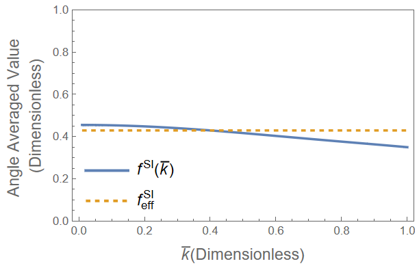
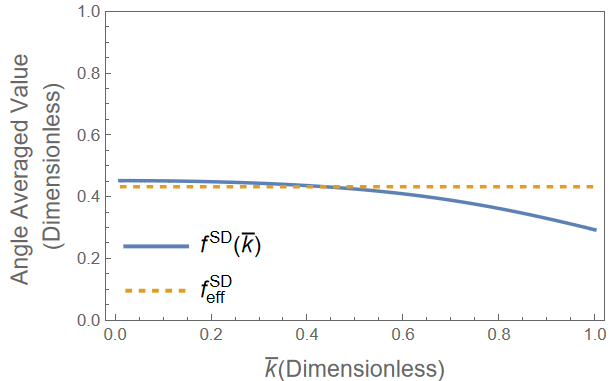
These functions depend not only on the magnitude of the dimensionless momentum transfer and average momentum , but on their relative angle. Fortunately, for the physically relevant values of these momenta, and do not vary significantly over the range of possible angular values. Therefore we may replace each function by its angular average. The angle-averaged functions then depend only on the magnitude of the momentum transfer and the average momentum . For a given nucleus, the three-momentum transfer in coherent conversion satisfies
| (79) |
where is the mass of the target nucleus and is the (positive) binding energy of the captured muon. Fixing the value of for a given nucleus, and become functions of the dimensionless average nucleon momentum , as shown in Fig. 4. In order to recover a local one-body effective operator, we replace these slowly-varying functions of by a constant, weighting our average by the single-nucleon momentum probability distribution. The resulting momentum-averaged values and are shown in Fig. 4. Table 1 reports the values of for the four nuclei of interest as well as the physical parameter values employed in each calculation.
References
- Petcov (1977) S. T. Petcov, The Processes in the Weinberg-Salam Model with Neutrino Mixing, Sov. J. Nucl. Phys. 25, 340 (1977), [Erratum: Sov.J.Nucl.Phys. 25, 698 (1977), Erratum: Yad.Fiz. 25, 1336 (1977)].
- Marciano and Sanda (1977a) W. J. Marciano and A. I. Sanda, Exotic Decays of the Muon and Heavy Leptons in Gauge Theories, Phys. Lett. B 67, 303 (1977a).
- Lee et al. (1977) B. W. Lee, S. Pakvasa, R. E. Shrock, and H. Sugawara, Muon and Electron Number Nonconservation in a V-A Gauge Model, Phys. Rev. Lett. 38, 937 (1977), [Erratum: Phys.Rev.Lett. 38, 1230 (1977)].
- Lee and Shrock (1977) B. W. Lee and R. E. Shrock, Natural Suppression of Symmetry Violation in Gauge Theories: Muon - Lepton and Electron Lepton Number Nonconservation, Phys. Rev. D 16, 1444 (1977).
- Baldini et al. (2016) A. M. Baldini et al. (MEG), Search for the lepton flavour violating decay with the full dataset of the MEG experiment, Eur. Phys. J. C 76, 434 (2016), arXiv:1605.05081 [hep-ex] .
- Bertl et al. (2006) W. H. Bertl et al. (SINDRUM II), A Search for muon to electron conversion in muonic gold, Eur. Phys. J. C 47, 337 (2006).
- Baldini et al. (2018) A. M. Baldini et al. (MEG II), The design of the MEG II experiment, Eur. Phys. J. C 78, 380 (2018), arXiv:1801.04688 [physics.ins-det] .
- Baldini et al. (2021) A. M. Baldini et al. (MEG II), The Search for + → e+ with 10–14 Sensitivity: The Upgrade of the MEG Experiment, Symmetry 13, 1591 (2021), arXiv:2107.10767 [hep-ex] .
- Bartoszek et al. (2014) L. Bartoszek et al. (Mu2e), Mu2e Technical Design Report 10.2172/1172555 (2014), arXiv:1501.05241 [physics.ins-det] .
- Abusalma et al. (2018) F. Abusalma et al. (Mu2e), Expression of Interest for Evolution of the Mu2e Experiment, (2018), arXiv:1802.02599 [physics.ins-det] .
- Abramishvili et al. (2020) R. Abramishvili et al. (COMET), COMET Phase-I Technical Design Report, PTEP 2020, 033C01 (2020), arXiv:1812.09018 [physics.ins-det] .
- Marciano and Sanda (1977b) W. J. Marciano and A. I. Sanda, The Reaction mu- Nucleus – e- Nucleus in Gauge Theories, Phys. Rev. Lett. 38, 1512 (1977b).
- Weinberg and Feinberg (1959) S. Weinberg and G. Feinberg, Electromagnetic Transitions Between mu Meson and Electron, Phys. Rev. Lett. 3, 111 (1959).
- Shanker (1979) O. U. Shanker, Dependence of Coherent Conversion Rate in Anomalous Neutrinoless Muon Capture, Phys. Rev. D 20, 1608 (1979).
- Czarnecki et al. (1998) A. Czarnecki, W. J. Marciano, and K. Melnikov, Coherent muon electron conversion in muonic atoms, AIP Conf. Proc. 435, 409 (1998), arXiv:hep-ph/9801218 .
- Kitano et al. (2002) R. Kitano, M. Koike, and Y. Okada, Detailed calculation of lepton flavor violating muon electron conversion rate for various nuclei, Phys. Rev. D 66, 096002 (2002), [Erratum: Phys.Rev.D 76, 059902 (2007)], arXiv:hep-ph/0203110 .
- Cirigliano et al. (2009) V. Cirigliano, R. Kitano, Y. Okada, and P. Tuzon, On the model discriminating power of mu — e conversion in nuclei, Phys. Rev. D 80, 013002 (2009), arXiv:0904.0957 [hep-ph] .
- Cirigliano et al. (2017) V. Cirigliano, S. Davidson, and Y. Kuno, Spin-dependent conversion, Phys. Lett. B 771, 242 (2017), arXiv:1703.02057 [hep-ph] .
- Davidson et al. (2018) S. Davidson, Y. Kuno, and A. Saporta, “Spin-dependent” conversion on light nuclei, Eur. Phys. J. C 78, 109 (2018), arXiv:1710.06787 [hep-ph] .
- Crivellin et al. (2017) A. Crivellin, S. Davidson, G. M. Pruna, and A. Signer, Renormalisation-group improved analysis of processes in a systematic effective-field-theory approach, JHEP 05, 117, arXiv:1702.03020 [hep-ph] .
- Davidson et al. (2019) S. Davidson, Y. Kuno, and M. Yamanaka, Selecting conversion targets to distinguish lepton flavour-changing operators, Phys. Lett. B 790, 380 (2019), arXiv:1810.01884 [hep-ph] .
- Davidson (2021) S. Davidson, Completeness and complementarity for and , JHEP 02, 172, arXiv:2010.00317 [hep-ph] .
- Rule et al. (2021) E. Rule, W. C. Haxton, and K. McElvain, Nucleon-level Effective Theory of Conversion, (2021), arXiv:2109.13503 [hep-ph] .
- Crivellin et al. (2014a) A. Crivellin, M. Hoferichter, and M. Procura, Improved predictions for conversion in nuclei and Higgs-induced lepton flavor violation, Phys. Rev. D 89, 093024 (2014a), arXiv:1404.7134 [hep-ph] .
- Bartolotta and Ramsey-Musolf (2018) A. Bartolotta and M. J. Ramsey-Musolf, Coherent conversion at next-to-leading order, Phys. Rev. C 98, 015208 (2018), arXiv:1710.02129 [hep-ph] .
- Weinberg (1979) S. Weinberg, Baryon and Lepton Nonconserving Processes, Phys. Rev. Lett. 43, 1566 (1979).
- Wilczek and Zee (1979) F. Wilczek and A. Zee, Operator Analysis of Nucleon Decay, Phys. Rev. Lett. 43, 1571 (1979).
- Buchmuller and Wyler (1986) W. Buchmuller and D. Wyler, Effective Lagrangian Analysis of New Interactions and Flavor Conservation, Nucl. Phys. B 268, 621 (1986).
- Grzadkowski et al. (2010) B. Grzadkowski, M. Iskrzynski, M. Misiak, and J. Rosiek, Dimension-Six Terms in the Standard Model Lagrangian, JHEP 10, 085, arXiv:1008.4884 [hep-ph] .
- Shifman et al. (1978) M. A. Shifman, A. I. Vainshtein, and V. I. Zakharov, Remarks on Higgs Boson Interactions with Nucleons, Phys. Lett. B 78, 443 (1978).
- Cirigliano et al. (2012) V. Cirigliano, M. L. Graesser, and G. Ovanesyan, WIMP-nucleus scattering in chiral effective theory, JHEP 10, 025, arXiv:1205.2695 [hep-ph] .
- Crivellin et al. (2014b) A. Crivellin, M. Hoferichter, and M. Procura, Accurate evaluation of hadronic uncertainties in spin-independent WIMP-nucleon scattering: Disentangling two- and three-flavor effects, Phys. Rev. D 89, 054021 (2014b), arXiv:1312.4951 [hep-ph] .
- Körber et al. (2017) C. Körber, A. Nogga, and J. de Vries, First-principle calculations of Dark Matter scattering off light nuclei, Phys. Rev. C 96, 035805 (2017), arXiv:1704.01150 [hep-ph] .
- Hoferichter et al. (2015) M. Hoferichter, J. Ruiz de Elvira, B. Kubis, and U.-G. Meißner, High-Precision Determination of the Pion-Nucleon Term from Roy-Steiner Equations, Phys. Rev. Lett. 115, 092301 (2015), arXiv:1506.04142 [hep-ph] .
- Aoki et al. (2021) Y. Aoki et al., FLAG Review 2021, (2021), arXiv:2111.09849 [hep-lat] .
- Alexandrou et al. (2014) C. Alexandrou, V. Drach, K. Jansen, C. Kallidonis, and G. Koutsou, Baryon spectrum with twisted mass fermions, Phys. Rev. D 90, 074501 (2014), arXiv:1406.4310 [hep-lat] .
- Durr et al. (2012) S. Durr et al., Sigma term and strangeness content of octet baryons, Phys. Rev. D 85, 014509 (2012), [Erratum: Phys.Rev.D 93, 039905 (2016)], arXiv:1109.4265 [hep-lat] .
- Durr et al. (2016) S. Durr et al., Lattice computation of the nucleon scalar quark contents at the physical point, Phys. Rev. Lett. 116, 172001 (2016), arXiv:1510.08013 [hep-lat] .
- Yang et al. (2016) Y.-B. Yang, A. Alexandru, T. Draper, J. Liang, and K.-F. Liu (xQCD), N and strangeness sigma terms at the physical point with chiral fermions, Phys. Rev. D 94, 054503 (2016), arXiv:1511.09089 [hep-lat] .
- Gupta et al. (2021) R. Gupta, S. Park, M. Hoferichter, E. Mereghetti, B. Yoon, and T. Bhattacharya, The nucleon sigma term from lattice QCD, (2021), arXiv:2105.12095 [hep-lat] .
- Freeman and Toussaint (2013) W. Freeman and D. Toussaint (MILC), Intrinsic strangeness and charm of the nucleon using improved staggered fermions, Phys. Rev. D 88, 054503 (2013), arXiv:1204.3866 [hep-lat] .
- Hoferichter et al. (2012) M. Hoferichter, C. Ditsche, B. Kubis, and U. G. Meissner, Dispersive analysis of the scalar form factor of the nucleon, JHEP 06, 063, arXiv:1204.6251 [hep-ph] .
- Brantley et al. (2016) D. A. Brantley, B. Joo, E. V. Mastropas, E. Mereghetti, H. Monge-Camacho, B. C. Tiburzi, and A. Walker-Loud, Strong isospin violation and chiral logarithms in the baryon spectrum, (2016), arXiv:1612.07733 [hep-lat] .
- Borsanyi et al. (2015) S. Borsanyi et al., Ab initio calculation of the neutron-proton mass difference, Science 347, 1452 (2015), arXiv:1406.4088 [hep-lat] .
- Bernard et al. (1992) V. Bernard, N. Kaiser, J. Kambor, and U. G. Meissner, Chiral structure of the nucleon, Nucl. Phys. B 388, 315 (1992).
- Moniz et al. (1971) E. J. Moniz, I. Sick, R. R. Whitney, J. R. Ficenec, R. D. Kephart, and W. P. Trower, Nuclear Fermi momenta from quasielastic electron scattering, Phys. Rev. Lett. 26, 445 (1971).
- Haxton et al. (2002) W. C. Haxton, C. P. Liu, and M. J. Ramsey-Musolf, Nuclear anapole moments, Phys. Rev. C 65, 045502 (2002), arXiv:nucl-th/0109014 .
- Johnson et al. (2013) C. W. Johnson, W. E. Ormand, and P. G. Krastev, Factorization in large-scale many-body calculations, Comput. Phys. Commun. 184, 2761 (2013), arXiv:1303.0905 [nucl-th] .
- Johnson et al. (2018) C. W. Johnson, W. E. Ormand, K. S. McElvain, and H. Shan, BIGSTICK: A flexible configuration-interaction shell-model code, (2018), arXiv:1801.08432 [physics.comp-ph] .
- Brown and Richter (2006) B. A. Brown and W. A. Richter, New ’USD’ Hamiltonians for the sd shell, Phys. Rev. C 74, 034315 (2006).
- Honma et al. (2002) M. Honma, T. Otsuka, B. A. Brown, and T. Mizusaki, Effective interaction for pf shell nuclei, Phys. Rev. C 65, 061301 (2002), arXiv:nucl-th/0205033 .
- Miller and Spencer (1976) G. A. Miller and J. E. Spencer, A Survey of Pion Charge-Exchange Reactions with Nuclei, Annals Phys. 100, 562 (1976).
- Rose (1961) M. E. Rose, Relativistic Electron Theory, John Wiley Sons, Inc., New York and London (1961).
- Strange (1998) P. Strange, Relativistic Quantum Mechanics, Cambridge University Press (1998).
- Silbar and Goldman (2011) R. R. Silbar and T. Goldman, Solving the radial Dirac equations: A Numerical odyssey, Eur. J. Phys. 32, 217 (2011), arXiv:1001.2514 [physics.comp-ph] .
- Garcia-Recio et al. (1992) C. Garcia-Recio, J. Nieves, and E. Oset, Neutron distributions from pionic atoms, Nucl. Phys. A 547, 473 (1992).
- De Vries et al. (1987) H. De Vries, C. W. De Jager, and C. De Vries, Nuclear charge and magnetization density distribution parameters from elastic electron scattering, Atom. Data Nucl. Data Tabl. 36, 495 (1987).
- Kitano et al. (2003) R. Kitano, M. Koike, S. Komine, and Y. Okada, Higgs mediated muon electron conversion process in supersymmetric seesaw model, Phys. Lett. B 575, 300 (2003), arXiv:hep-ph/0308021 .
- Kim et al. (1997) J. E. Kim, P. Ko, and D.-G. Lee, More on R-parity and lepton family number violating couplings from muon(ium) conversion, and tau and pi0 decays, Phys. Rev. D 56, 100 (1997), arXiv:hep-ph/9701381 .
- Huitu et al. (1998) K. Huitu, J. Maalampi, M. Raidal, and A. Santamaria, New constraints on R-parity violation from mu e conversion in nuclei, Phys. Lett. B 430, 355 (1998), arXiv:hep-ph/9712249 .
- Faessler et al. (2000) A. Faessler, T. S. Kosmas, S. Kovalenko, and J. D. Vergados, Constraints on R-parity violating supersymmetry from muon electron nuclear conversion, Nucl. Phys. B 587, 25 (2000), arXiv:hep-ph/9904335 .
- de Gouvea et al. (2001) A. de Gouvea, S. Lola, and K. Tobe, Lepton flavor violation in supersymmetric models with trilinear R-parity violation, Phys. Rev. D 63, 035004 (2001), arXiv:hep-ph/0008085 .
- Harnik et al. (2013) R. Harnik, J. Kopp, and J. Zupan, Flavor Violating Higgs Decays, JHEP 03, 026, arXiv:1209.1397 [hep-ph] .
- Barr and Zee (1990) S. M. Barr and A. Zee, Electric Dipole Moment of the Electron and of the Neutron, Phys. Rev. Lett. 65, 21 (1990), [Erratum: Phys.Rev.Lett. 65, 2920 (1990)].
- Abe et al. (2014) T. Abe, J. Hisano, T. Kitahara, and K. Tobioka, Gauge invariant Barr-Zee type contributions to fermionic EDMs in the two-Higgs doublet models, JHEP 01, 106, [Erratum: JHEP 04, 161 (2016)], arXiv:1311.4704 [hep-ph] .
- Bernstein (2019) R. H. Bernstein (Mu2e), The Mu2e Experiment, Front. in Phys. 7, 1 (2019), arXiv:1901.11099 [physics.ins-det] .
- Prezeau et al. (2003) G. Prezeau, M. Ramsey-Musolf, and P. Vogel, Neutrinoless double beta decay and effective field theory, Phys. Rev. D 68, 034016 (2003), arXiv:hep-ph/0303205 .