PiDAn: A Coherence Optimization Approach for Backdoor Attack Detection and Mitigation in Deep Neural Networks
Abstract
Backdoor attacks impose a new threat in Deep Neural Networks (DNNs), where a backdoor is inserted into the neural network by poisoning the training dataset, misclassifying inputs that contain the adversary trigger. The major challenge for defending against these attacks is that only the attacker knows the secret trigger and the target class. The problem is further exacerbated by the recent introduction of “Hidden Triggers,” where the triggers are carefully fused into the input, bypassing detection by human inspection and causing backdoor identification through anomaly detection to fail.
To defend against such imperceptible attacks, in this work we systematically analyze how representations, i.e., the set of neuron activations for a given DNN when using the training data as inputs, are affected by backdoor attacks. We propose PiDAn, an algorithm based on coherence optimization purifying the poisoned data. Our analysis shows that representations of poisoned data and authentic data in the target class are still embedded in different linear subspaces, which implies that they show different coherence with some latent spaces. Based on this observation, the proposed PiDAn algorithm learns a sample-wise weight vector to maximize the projected coherence of weighted samples, where we demonstrate that the learned weight vector has a natural ”grouping effect” and is distinguishable between authentic data and poisoned data. This enables the systematic detection and mitigation of backdoor attacks. Based on our theoretical analysis and experimental results, we demonstrate the effectiveness of PiDAn in defending against backdoor attacks that use different settings of poisoned samples on GTSRB and ILSVRC2012 datasets. Our PiDAn algorithm can detect more than 90% infected classes and identify 95% poisoned samples.
Index Terms:
Deep Neural Networks (DNNs), Backdoor Attacks, Backdoor Defense, Optimization, Machine Learning SecurityI Introduction and Related Work
Backdoors in Deep Neural Networks (DNNs) are a recent insidious attack [1, 2, 3, 4, 5, 6]. These attacks aim to insert a backdoor inside of the target DNN model so that the attacker can control the model output (typically the class label) when triggered using a specific input pattern. Data poisoning is an effective way to implement this attack, where the poisoned samples with the attacker-chosen properties (e.g., patched with specific triggers) are added to the genuine training dataset and labeled as the target class. After training on the mixture of genuine and poisoned data, the backdoored model can connect the attacker-chosen properties to the target label and also hold high accuracy on clean test samples. Since its discovery in 2017, there has been a plethora of research with attack literature focusing on developing stealthier attacks and defense literature developing schemes to protect models against those specific attacks. The defense mechanisms typically analyze the properties of backdoor triggers (attack signatures) to distinguish between benign and malicious instances. In this work, we take a different approach in comparison to the state-of-the-art defenses, shifting the focus to fundamental properties of DNNs instead of trigger-specific properties.
The major challenge of developing a generalizable defense is that the trigger space is infinite, making its analysis cumbersome. In DNNs, deeper layers can extract underlying features of complex data, which transforms the input data associated to different objects to linearly separable representations, i.e., the set of neuron activations for a given DNN when using the training data as inputs. The features associated to different objects lie in different latent linear subspaces [7, 8]. This is a fundamental property of DNNs. In a backdoored network, even though the poisoned data is manually assigned the label of one object, their features are different, i.e., intuitively the representations for poisoned data and the genuine/clean data lie in two different linear subspaces. Defense mechanisms leveraging the inherent DNN characteristics have the added advantage of being attack-agnostic, i.e., their detection capability can be consistent across different datasets as well as different attack algorithms.
|
|
|
|
|
|
|
|
| |||||||||||||||||||||
| Partial backdoor defense | ✓ | ✓ | ✓ | ✓ | |||||||||||||||||||||||||
| Hidden trigger defense | ✓ | ✓ | |||||||||||||||||||||||||||
| Backdoor detection | ✓ | ✓ | ✓ | ✓ | ✓ | ✓ | ✓ | ||||||||||||||||||||||
| Model recovery | ✓ | ✓ | ✓ | ✓ | ✓ |
Initial work on backdooring neural networks studied the feasibility of backdoor attacks using small patches as triggers [17, 18, 19]. Following that line of work, researchers identified that these attacks are based on a strong connection between the trigger and the output, and formed mitigation strategies for detecting the backdoors based on the trigger dominance. In order to break the dominance of triggers, Tang et al., [14] proposed to not only add patched data to the target classes, but also add covering data (data from non-source classes patched with triggers) to their original classes. In this manner, only the output of the trigger-carrying source data can be flipped by the triggers. They also show that, in their case, the representations of the authentic data and the poisoned data overlap significantly, which makes it difficult to detect the poisoned data. The more advanced clean-label backdoor attack [20] and hidden trigger backdoor attack [21] generate poisoned samples that can be naturally labeled as the target class, i.e., they look like samples from the target class.
The existence of backdoors in a model is not reflected in the regular performance metrics like test accuracy. Therefore, defense literature focuses on analyzing the potential trigger properties (e.g., strong connection with the output labels) in order to perform backdoor detection [22, 23, 24, 25, 26, 27, 28]. Defenses can be broadly classified in two categories: (1) Methods that focus on the connection between the trigger and the output, and (2) Methods that focus on distinguishing poisoned samples from clean samples in the training set. We first summarize the functionality of the state-of-the-art defense methods in Table I, and then further analyze each category.
With regards to the defense literature that examines the strong connection between the trigger and the output, the backdoor can be detected by restoring a small pattern that can cause any image to be misclassified as the target [10], or the small region on image that is significantly important for classification [29], or small range of neurons stimulated by triggers [11]. More specifically, Neural Cleanse [10] and Deepinspect [30] detect the existence of backdoor by reverse-engineering the trigger pattern that can misclassify all images attached with this trigger pattern to each target class. For the backdoored model, the trigger pattern for the true infected class will be much smaller than that of the uninfected ones in magnitude. This type of defense can discover the trigger by accessing the victim models. However, it is computationally expensive to reverse engineer the trigger pattern for each class, especially for a large number of classes. Furthermore, their performance is also constrained by the size of the triggers. ABS [11] assumes that a set of inner neurons within the certain range will be triggered since the trigger representations will dominate the misclassification. They detect the poisonous neurons by stimulating the clean images. However, this method shows less effectiveness for some emerging attacks [21, 14] which break the dominance of the trigger. STRIP [12] and SentiNet [13] aim to detect poisonous images in the testing phase. These two methods hold the same limitation as ABS, which relies on the dominance of triggers for misclassification. Finally, authors in [9] fuzz the input and perform majority voting to suppress the backdoor. This method, however, is not capable of detecting the existence of backdoors in the model, and incurs performance overhead for clean and backdoored models indistinguishably.


The above defense methods are effective when all images with triggers are misclassified. Therefore, in order to detect ”partial” backdoors, where only images from some classes are triggered, recent literature focuses on the fact that the poisoned data and authentic data receive the same output class for different reasons [16], thus, their learned representations show different characteristics. These methods [16, 14, 15] utilize anomaly detection techniques [31, 32, 33, 34] to detect the existence of poisoned samples with the assumption that they depart from their non-poisoned counterparts, especially in the representation space [16], and they are still effective even if the trigger is fused with other clean features for classification. Within this category, Activation Clustering (AC) [16] and SCAn [14] detect the infected class by distinguishing the poisoned and authentic samples. AC focuses on the Independent Component Analysis (ICA) principal components of the representations for each class. They assume that the top principal components of the data in the infected class fall into two separable clusters, the poisoned one and the authentic one. Then they can detect the infected class and access the poisoned samples for repairing the malicious model. Instead of directly distinguishing two clusters of representations, SCAn recovers the representation distribution for each class. The representations from the authentic class follow single Gaussian distribution and representations in the infected class follow two Gaussian mixture (the authentic and the poisoned). It should be noted that, to simplify the problem, they assume the poisoned and the authentic representations in the infected classes both follow the Gaussian distributions with the same variance and different means. Thus, the difference between the poisoned and authentic distributions relies on their different means. Spectral signature [15] also falls into this category. It removes the samples having large correlations with the top principal components of the corrupted data, which in turn have high probability of departing distribution of the authentic data. Despite of the effectiveness of above methods, they might face challenges when learned features are not well shaped, i.e., they don’t have clear clusters. To illustrate this, we present the distributions of the top principal components with respect to poisoned and authentic representations in Figure 1a, where the representations are obtained by feeding the poisoned dataset (from GTSRB, under hidden trigger attack) into the DNN. In Figure 1b, we also present the classification results via support vector machine (SVM) based on the principal components as the core technique of above methods is classification/clustering upon learned features. For SVM, we assume the labels of poisoned and authentic representations are known. It is noted that undesired classification results are obtained, e.g., too many misclassified points, since the principal components are not well separated. This implies traditional defense methods might fail in these scenarios.
To this end, we design a novel poisoned data analysis based method, PiDAn, which utilizes data coherence to extract more abstract and discriminant features, i.e., a weight vector, based on which authentic and poisoned representations can be clearly indicated. Poison purifying (e.g., detection and mitigation of backdoor attacks) is further realized by implementing likelihood ratio test based algorithm and clustering technique. Our novel contributions are summarized as follows:
- 1.
We study how backdoor attacks affect representations of DNNs, where our findings show that the representations of authentic data and poisoned data in the target class are embedded in different linear subspaces, which implies they showcase different coherence with the latent spaces.
- 2.
We propose the PiDAn algorithm, which is based on a coherence optimization problem. It learns a sample-wise weight vector via maximizing the projected coherence of weighted samples. The learned weight vector is demonstrated to have a natural ”grouping effect” and is distinguishable between authentic data and poisoned data, which implies that the PiDAn algorithm can successfully detect and mitigate backdoors.
- 3.
We test our method on state-of-the-art neural networks, e.g., Alexnet, with wide range of visual recognition applications, from general object identification to specific traffic sign recognition, using basic and advanced trigger designs. We also compare our method with state-of-the-art methods, i.e., Spectral Signature, Activation Clustering and SCAn, to demonstrate the efficacy and benefits of our proposed method in detecting infected classes and identifying poisoned samples.
II Threat Model
Our threat model considers an attacker who can manipulate the training dataset by adding poisoned samples, but does not interfere with the training process and/or the model parameters. Such an attack scenario has been adopted by recent work such as Hidden Trigger [21], TaCT [14], and Badnets [17]. In this scenario, attacks can originate from the data source provider (i.e. data coming from untrusted sources), or from intruders or insiders who can stealthily inject poisoned samples into the collected training set [26, 14].
More precisely, the objective of the attacker is to insert backdoors into a victim DNN and produce a backdoored DNN , which holds the following properties: (1) misclassifies the source samples patched with the attacker-selected trigger to the target class, that is; (2) maintains high test accuracy on clean test samples so as not to be detected by monitoring the test accuracy. The backdoor is inserted by data poisoning, and the DNN is trained on the mixture of the triggered dataset (added by the attacker) and the genuine dataset , i.e., , generating the malicious model. As mentioned earlier, the attacker has full control of changing the data that are used for the training but has no direct access to manipulate the model parameters and the training process.
In this work, we consider the following attacks:
- 1.
Hidden trigger: Hidden trigger backdoor attack [21] is one of the latest backdoor attacks. In this scenario, the attacker identifies poisoned images that are similar to the target in the image space but are close to the patched source, i.e., source images with triggers, in the representation space, and adds them to the genuine dataset. In this way, the poisoned images in the target class can bypass human inspection while the malicious model can still succeed in misclassifying the patched source images to the target label. The authors showed that the conventional statistical anomaly detection methods failed to detect the poisoned data since their representations fuse with those of the genuine target data, exhibiting less separation.
- 2.
TaCT: It was first proposed in [14], adding not only patched source images but also cover images, i.e., images from other classes attached with triggers, to the genuine dataset so as to weaken the dominance of the triggers and to obscure the difference between the poisoned data and target data. In this attack, 1 of the genuine images patched with the triggers are also added to the clean dataset as covering images.
- 3.
Badnets [17]: It is the conventional backdoor strategy where the patched source images with the target label are added to the genuine training dataset for manipulating the DNNs.
On the defender side, similar to the state-of-the-art defense techniques based on training data inspection, e.g., Activation Clustering [16], SCAn [14], and Spectral Signatures [15], we assume that defenders have full access to the training data and the model under test so that they can collect the representations for each input sample, but they have no information about the poisoned data, for example the shape or position of the trigger. Furthermore, defenders have no control or visibility to the training process.
III Preliminaries
In this section, we begin by defining and analyzing the representations that motivate our defense.
Representations: We denote the representations as the neuron activations learned by the layers of a neural network with given inputs. Formally, let be an input sample and denote the mapping from -th layer to -th layer , then the representations from the th layer is defined as . For simplicity, we drop the superscript and denote as .
Properties of representations: A well-trained deep architecture can learn the underlying factors of variations determining the geometrical structure of raw data (inputs) [7]. In this sense, data structures are flattened across layers. Especially, at the last layer, representations lie on a Euclidean space, a.k.a. a linear space.
| Layers | Flattening metric | |
| Stop sign | speed limit | |
| Input layer | 0.2219 | 0.3278 |
| Intermediate layer | 0.1551 | 0.2499 |
| Last layer | 0.0411 | 0.0831 |
To illustrate the above properties, we use a flattening metric which is adapted from [8] (please see Appendix B for details). This metric is derived from the difference between geodesic and Euclidean distances. It should be equal to 0 when the data lie exactly in a linear space (since the geodesic and Euclidean distances are equal). We compute the metric using the representations from each layer of the respective DNNs. As an example, let us consider the GTSRB dataset and the corresponding 6Conv+2Dense network and present the flattening metric for the input layer, an intermediate layer, and the last layer in Table II. It can be observed that the value of the flattening metric decreases with increase in the depth of the network, and the values of the last layer are small enough (close to 0), indicating representations from the last layer almost lie in a linear subspace.
Remark 1. It is reasonable to assume representations of higher/deeper layers (especially the last layer) for each object/class approximately lie on a Euclidean subspace, i.e., a linear subspace.
This motivates us to focus on the representations of the last layers of the network, where processing becomes easier than on raw inputs, since, for example, linear techniques can be used.
| (Target poisoned) | Flattening metric | SVM | |
| Target | Poisoned | ||
![[Uncaptioned image]](2203.09289v2/Imgs/60c.png)
|
0.0831 | 0.0844 | 70.85 |
![[Uncaptioned image]](2203.09289v2/Imgs/5c.png)
|
0.0978 | 0.1102 | 77.18 |
![[Uncaptioned image]](2203.09289v2/Imgs/62c.png)
|
0.0775 | 0.0838 | 68.18 |
The signal (malicious activation) corresponding to triggers get boosted as we advance through the layers of the DNN [15]. In other words, deeper layers manifest the trigger properties more conspicuously than earlier layers. Another line of research observed that the backdoored models tend to assign poisoned samples and benign samples to target classes based on different sets of features [16]. For the benign samples, the output is based on the inherent features of the (true) target class; but for the poisoned samples, the final classification is influenced by the trigger features, which is different from the inherent features. Therefore, considering the infected target class, the samples (and their representations) belonging to this class can be viewed as a mixture of two groups: The poisoned samples and the benign samples [14]. In this case, despite that the poisoned data and authentic data receive the same classification label, their mechanism of classification are different and this difference should be evident in the representations. Wang et al. [10] also indicates that backdoored networks classify the poisoned data to the target class regardless of its original class mainly by changing the decision boundaries (instead of focusing on representation fusion). Besides the boundary change, the representations of the poisoned data can also fuse with those of the authentic data for some advanced attacks, e.g., dynamic trigger attacks and hidden trigger backdoor attacks, which makes it hard to group the representations into two distinct clusters and introduce more challenges for backdoor detection.


Furthermore, we observe that the representations of authentic data and poisoned data are still embedded in different linear spaces despite limited separation. To verify this observation, Table III summarizes the flattening metric values as well as the linear separability for three data pairs (e.g., each pair includes target class and poisoned class) in the last layer of backdoored network, where the linear separability is evaluated by the classification accuracy of support vector machine (SVM). We can see all their flattening metric values are small, indicating each class approximately lies in linear spaces. At the same time, classification accuracy based on SVM is not high, which implies that they cannot be clearly separated by linear techniques. Moreover, we present in Fig. 2 that the spectral signature [15] of authentic representations and poisoned representations do not separate enough, since their correlations with the top eigenvector of the covariance matrix of representations are similar. This leads to our the second assumption:
Remark 2. The representations of authentic data and poisoned data from the last layer still lie approximately on different linear subspaces, which are not clearly separated.
Data model: Given a set of data points (without further declaration, we denote by data the representations/activations from the last layer of the DNN) in , denoted by , which is the mixture of the targeted/authentic set and the poisoned/trigger set, we assume that
| (1) |
where denotes the targeted/authentic dataset and is the poisoned/trigger dataset; and .
Our data model is then:
| (2) |
or
| (3) |
where consists of samples of representations of dimensionality from the set , and denotes a column of . The component represents the object-specific representations (belonging to object ) containing critical information for discrimination, and . On the contrary, (without superscript) is a column of containing common/global information shared by different objects. We can also denote or as noise/perturbation that is useless for classification. Furthermore, we designate the following conditions w.r.t. the data model:
Condition 1: Each object-specific representation, e.g., or , perfectly lies in a linear subspace, e.g., or , which has low rank structure; By contrast, each global representation is independent identical distributed (i.i.d.) and is uncorrelated to object-specific ones, e.g., and .
More specifically, Condition 1 implies that any pair satisfies , where the rationale is that if then contains useful information for classification which can be incorporated into .
IV Methodology
IV-A Insight of the proposed algorithm
Our proposed algorithm takes the advantage of the property that representations of authentic data and poisoned data approximately lie on different linear subspaces. We designate and solve a convex optimization problem which maximizes the coherence of weighted samples and a certain subspace, so as to obtain a sample-wise weight vector where its entries are well separated according to their associated subspace affiliations. The poisoned data can thus be detected and identified based on this weight vector, and finally mitigation of backdoor attacks can be realized.
We give an example to illustrate the intuition of the proposed algorithm. For simplicity, we consider a noiseless case where representations perfectly lie in their associated subspaces. However, it should be noted that the conclusion drawn from noiseless case still holds for noisy case as perturbation/noise is uncorrelated with the object-specific components. Consider two subspaces and , and two associated datasets of representations, i.e., and , where denotes the authentic data and denotes the poisoned data. All samples are scaled to unit length, and all features are centralized using the information from clean testing data. Denote and the orthonormal basis matrix spanning and , respectively. Let , and the sample-wise weight vector be the optimal solution of the following optimization problem
| (4) |
The optimization problem (4) searches a unit weight vector that maximizes the coherence between weighted samples, i.e., , and a projected subspace, i.e., where . Since is orthogonal to , any samples from make no contribution to increasing the coherence between weighted samples and . Thus, the above optimization problem is more likely to assign small weights to and give large weights to . To illustrate this, an extreme case is if all weights corresponding to are non-zeros and others are zeros, the objective value of (4) would be zero. In this way, there would exist a distinct gap between the weights associated with different datasets, which enables the detection and identification of poisoned dataset () by analyzing , e.g., using clustering techniques.
This intuition is illustrated in Fig. 3, which shows two subspaces and along with a subspace that is orthogonal to . If and are orthogonal to each other, then data points from have zero coherence with the subspace .

IV-B Problem Formulation and Optimization
We then extend the optimization problem in Eq.(4) to a more generalized case, where the ground truth labels (e.g., which class they originally come from) of and are unknown. We estimate a projection matrix which is expected to be closer to than , so that a sample from contributes less to the objective function than a sample from . Correspondingly, it is more likely to assign larger weights to than , and thus there would be a gap in the weights of the sample-wise weight vector . Given a proper , we formulate the following optimization problem
| (5) |
where , denotes the authentic data and denotes the poisoned data. All samples are scaled to unit length, and all features are centralized by the information from clean testing data.
As Eq.(5) is in fact an eigenvalue decomposition problem which is tractable, the optimal could be directly obtained by performing eigenvalue decomposition of , and is the eigenvector corresponding to the largest eigenvalue. It is noted that plays an important role in above optimization problem, More specifically, we demonstrate in our experiments that the smaller the angle between and , the larger the gap between the weights w.r.t. and . Then, we propose a simple way to calculate in the backdoor attack scenario where the variations of poisoned representations are more likely to be smaller than those of the authentic ones in the target class (this may be attributed to the sample size of poisoned samples as well as the stealthy objective of backdoor attack). We perform an eigenvalue decomposition on the mixture representations in the target class and select the first eigenvectors as .
IV-C Detection and Mitigation based on Sample-wise Weight Vector
The intuitive idea behind detection is that, the elements of would be bi-modal if the representations are contaminated, which is because of the aforementioned gap in the weights of samples from two groups, the genuine and the poisoned; on the contrary, the elements of would be uni-modal if the representations are not contaminated.
To this end, we adopt likelihood ratio test [35] to judge whether the representations are contaminated or not. If a uni-modal distribution such as a single Gaussian fits better, the corresponding class is authentic; if a bi-modal distribution like the mixture of two Gaussian fits better, the corresponding class is infected. More precisely, for each class , we test the following null hypothesis,
: is drawn from a Gaussian distribution;
: is drawn from a two-component Gaussian mixture distribution.
The test is based on the following statistic:
| (6) |
where denotes the estimated likelihood of under the null hypothesis, and represents the likelihood of under the alternative hypothesis. It should be noting that the likelihood functions are estimated by EM algorithm [36].
The statistic follows a chi-square distribution with the degrees of freedom being equivalent to the difference of free parameters between the two hypothesis [35]. Since is not symmetrically distributed, we use the technique based on a robust scale estimator, Absolute Pairwise Difference (APD) [37], to detect the class with great values of . More precisely, we further compute the following statistic, which is termed as anomaly index, for each class
| (7) |
where denotes the sample median and is the correct factor making APD unbiased towards finite samples. In this way, we flag those as spurious for which exceeds a threshold () with confidence level . Furthermore, we focus on those classes with . The specific procedures of the detection algorithm are summarized in Algorithm 1.
In the following stage, we identify those poisoned data points and remove them to achieve backdoor attack mitigation. Our identification method is derived based on the following property,
Remark 3. The optimized weights have a grouping effect. More precisely, let be the solution of Eq.(5), we have
| (8) |
where is the square of the maximum eigenvalue of , and are elements of , and denotes the coherence between samples. See Appendix A for more details.
Since is the largest eigenvalue of , which is much larger than 1 in practice (as derived from different classes from ILSVRC2012 and GTSRB datasets, ranges from 15 to 30), it is easy to observe that the difference between and is extremely small (close to 0) when and are highly correlated ( is close to 1).
Remark 3 provides a theoretical guarantee that highly correlated data points can be grouped into the same cluster by analyzing the weight vector. Again, we have demonstrated that there is distinct gap among the entries of the weight vector. These jointly implies, the identification of poisoned samples could thus be achieved by using the state-of-the-art clustering algorithms. In this work, the simple clustering algorithm, i.e., ”k-means” [38] can well separate the poisoned samples from the authentic ones based on our optimized weight vector, which also highlight the effectiveness of the proposed coherence optimization algorithm. We summarize the identification and mitigation procedure in Algorithm 2.
| (9) |
| (10) |
IV-D Computational Complexity
Since the proposed coherence optimization problem in Eq.(5) can be solved by a simple eigenvalue decomposition on , its computational complexity is . For the detection algorithm, the major computational burden is produced by the EM algorithm that is used to estimate the likelihood function in each hypothesis. The complexity of EM algorithm is generally , where is the sample size and is the iteration steps. For the mitigation algorithm, the computational complexity of ”k-means” is typically . The overall complexity of our method is .
V Experimental Results
In this section, we evaluate our backdoor detection scheme on the ILSVRC2012 dataset [39] (built for recognizing general objects) and GTSRB dataset [40] (built for recognizing traffic signs) for three attack schemes: (1) Hidden trigger [21]; (2) TaCT [14]; and (3) Badnets [17]. We use AlexNet [41] for the ILSVRC2012 dataset, and a simplified network of 6 convolution layers and 2 dense layers (see Table XIV in the Appendix) for the GTSRB dataset. For each infected model, we use the randomly generated square triggers in [21] as shown in Fig 4. For the ILSVRC2012 dataset, the trigger is of size with varying positions. Since the input size of the GTSRB dataset is only , we set the trigger size as and fix it at the bottom right corner of the images. The adopted experimental method follows well-established evaluation methods in the state-of-the-art [21, 10, 14].


V-A Infected models
V-A1 Random ILSVRC2012 source-target pairs
We choose 10 random pairs of source and target categories from ILSVRC2012 to evaluate our defense strategy. We use 800 genuine images for each class and add 400 poisoned samples to the target class, similar to hidden trigger attack setup [21]. The classification accuracy (CA) and the attack success rates (ASRs) are summarized in Table V. In summary, the infected models can achieve comparable classification accuracy as the clean models and the ASRs are above 70% for hidden trigger attacks and around 90% for the TaCT and badnets.
V-A2 Selected GTSRB source-target pairs
We also evaluate our method on the GTSRB dataset for showing how our method defends against backdoor attacks in traffic sign identification models. We choose three source-target pairs which will cause life-risking threats in real world. The GTRSB pairs are listed in Table IV. We add 800 poisoned samples for each source-target pairs. It is noted that we also pick two speed limit signs (speed limit of 30 and 80) with similar features, so that we can evaluate how our defense works for similar target and source classes. The performance of the clean and infected models are summarized in Table V. In general, the infected models hold high classification accuracy and high attack success rate.
| source | target |
![[Uncaptioned image]](2203.09289v2/Imgs/14.png)
|
![[Uncaptioned image]](2203.09289v2/Imgs/3.png)
|
| stop sign | speed limit of 60 |
![[Uncaptioned image]](2203.09289v2/Imgs/1.png)
|
![[Uncaptioned image]](2203.09289v2/Imgs/5.png)
|
| speed limit of 30 | speed limit of 80 |
![[Uncaptioned image]](2203.09289v2/Imgs/17.png)
|
![[Uncaptioned image]](2203.09289v2/Imgs/13.png)
|
| no entry | yield |
| Attack Type | ILSVARC2012 | GTSRB | |||||
| clean | Infected | clean | Infected | ||||
| CA | CA | ASR | CA | CA | ASR | ||
| Hidden trigger | 93.5% | 92.7% | 78.2% | 96.7% | 96.0% | 84.1% | |
|
93.5% | 92.7% | 88.7% | 96.7% | 96.1% | 96.4% | |
| Badnets | 93.5% | 93.0% | 90.5% | 96.7% | 96.5% | 96.5% | |
V-B Performance of the proposed defense
In this section, we specify the steps of implementing our defense as described in Section IV, including identifying the infected class based on the optimized weights and locating the poisoned samples by clustering the weights. The infected models can be repaired by our method by removing the poisoned samples and retraining the model from scratch or relabeling the poisoned samples with their source class and continuing the training. Experiments are performed on a 2.9 GHz Intel i7 processor with 32 GB of RAM.
V-B1 Infected class detection via optimized sample weights


First, we evaluate how accurately our defense can identify the infected classes. In our methodology, we aim to distinguish the representations of the poisoned samples from those of the clean samples, which can significantly overlap (see Fig 7a), and thus are hard to separate into two corresponding groups by conventional clustering methods, like KNN and K-means.
Based on Eq. (5), the optimized sample weight vector can be calculated based on the learned representations for each class. For the infected class, it is obvious that the weights for the authentic and poisoned samples form two distinguishable clusters, while the weights for the clean class almost follow the Gaussian distribution. The optimized weights for the infected and clean class are shown in Fig 5, from which we can see different distributions of the optimized weights in infected class and clean class.
Then, for each class, we fit the distribution of optimized weights via the mixture of Gaussian distribution(s) with different number of kernel(s) and report the likelihood ratio along with the anomaly index defined in Eq. (7). The anomaly index for one class exceeding a threshold () indicates that this class is infected with corresponding confidence level. As suggested by [42], we vary the threshold () using the values [2, 2.5, 3], which means the confidence level of the optimized weight vector drawn from a two-component of mixture normal distribution –that is, the corresponding class is infected– varies from to . More specifically, [42] suggests a threshold of 2.5 as a conservative choice for univariable statistical problems, with 3 being ”very conservative” and 2 ”poorly conservative” choices respectively. The detection rates are summarized in Table VI. We observe our PiDAn algorithm can achieve superior backdoor detection performance with infected class detection rates around 96% and less than 5.5% clean classes being misclassified as the infected. Shown in Fig 6, the anomaly index of infected classes all exceed 3, but the indexes for the hidden trigger attack are much smaller than those of the other two attacks, which indicates the representations of poisoned and clean data for hidden trigger attack are less separable than the others and it is harder to be detected.
| Detection Method | ILSVARC2012 | GTSRB | ||||||||||
| Hidden trigger | TaCT | Badnets | Hidden trigger | TaCT | Badnets | |||||||
| TPR | FPR | TPR | FPR | TPR | FPR | TPR | FPR | TPR | FPR | TPR | FPR | |
| AC-0.10 | 50.0% | 39.5% | 50.0% | 38.4% | 51.0% | 38.4% | 76.6% | 60.2% | 100.0% | 62.4% | 100.0% | 59.5% |
| AC-0.11 | 10.0% | 32.6% | 46.0% | 31.6% | 48.0% | 31.1% | 60.0% | 47.1% | 66.7% | 45.5% | 66.7% | 44.8% |
| AC-0.12 | 5.0% | 20.1% | 10.0% | 21.6% | 8.0% | 19.5% | 33.3% | 34.8% | 63.3% | 35.5% | 66.7% | 32.4% |
| AC-0.13 | 4.0% | 14.2% | 5.0% | 16.3% | 5.0% | 15.8% | 30.0% | 34.8% | 53.3% | 33.1% | 60.0% | 30.1% |
| AC-0.14 | 0.0% | 6.8% | 5.0% | 6.3% | 5.0% | 5.3% | 16.7% | 25.2% | 16.7% | 23.6% | 26.7% | 24.5% |
| AC-0.15 | 0.0% | 0.0% | 0.0% | 0.0% | 3.0% | 2.6% | 3.3% | 19.5% | 3.3% | 18.6% | 3.3% | 18.8% |
| SCAn | 83.0% | 6.8% | 96.0% | 5.3% | 100.0% | 4.2% | 96.7% | 5.9% | 96.7% | 4.8% | 100.0% | 5.2% |
| PiDAn-2 | 92.0% | 13.2% | 98.0% | 12.6% | 100.0% | 12.1% | 96.7% | 10.7% | 100.0% | 11.0% | 100.0% | 9.8% |
| PiDAn-2.5 | 92.0% | 8.9% | 98.0% | 9.5% | 100.0% | 8.4% | 96.7% | 7.9% | 96.7% | 7.4% | 100.0% | 7.4% |
| PiDAn-3 | 88.0% | 2.1% | 98.0% | 2.1% | 100.0% | 1.6% | 96.7% | 5.2% | 96.7% | 5.5% | 100.0% | 4.0% |


V-B2 Poisoned samples identifying via K-means
It is important to identify the poisoned samples for further analyzing the backdoor attack and mitigating its influence in deep learning models after the infected classes are detected. Based on Section IV-B, the optimized weight vector for the infected class is further clustered into two classes by K-means and the clusters with less samples is considered to be the poisoned samples with high probability. We summarize the rates of located poisoned samples in Table VII. It is noted that our method can identify the poisoned with high accuracy and identify few genuine samples as the poisoned. For the case of similar source and target (speed limit 30 and speed limit 80), whose representations are shown in Fig 7a, our method can achieve high poisoned sample identification accuracy, e.g., identify 90% poisoned samples as shown in Fig 7b, which is sufficient to suppress the backdoor influence after removing these poisoned samples.


| Defense Method | ILSVARC2012 | GTSRB | ||||||||||
| Hidden trigger | TaCT | Badnets | Hidden trigger | TaCT | Badnets | |||||||
| TPR | FPR | TPR | FPR | TPR | FPR | TPR | FPR | TPR | FPR | TPR | FPR | |
| AC [16] | 74.6% | 10.1% | 74.9% | 11.5% | 80.3% | 7.4% | 82.4% | 12.6% | 82.9% | 16.5% | 71.4% | 14.0% |
| SCAn [14] | 64.8% | 33.4% | 65.1% | 34.5% | 65.8% | 32.6% | 33.1% | 51.5% | 33.4% | 52.2% | 35.0% | 52.1% |
| PiDAn | 95.8% | 4.4% | 95.2% | 3.0% | 96.5% | 3.0% | 97.7% | 12.0% | 97.5% | 13.4% | 98.5% | 11.9% |
V-B3 Backdoor mitigation via poison samples exclusion
As suggested in [16], after identifying the poisoned samples, we can remove these samples from the target class and retrain the model. The performance of the repaired models are summarized in Table VIII. It shows that the repaired models hold comparable classification accuracy since the test errors for the genuine samples are similar before and after removing the identified suspicious samples and repairing the backdoored models. Besides, the backdoor influences are successfully mitigated since less than 10% of the source images carrying triggers are classified as the target. Specifically, for the case shown in Fig 7, the test errors of the repaired model for the genuine and poisoned samples are 4.0% and 9.5% respectively.
| ILSVARC2012 | GTSRB | |||||||||||||
| Pair ID | 1 | 2 | 3 | 4 | 5 | 6 | 7 | 8 | 9 | 10 | 1 | 2 | 3 | |
| Before | G | 7.3% | 7.5% | 7.3% | 7.3% | 7.2% | 7.3% | 7.4% | 7.6% | 7.6% | 7.3% | 3.7% | 4.0% | 3.7% |
| P | 93.1% | 70.8% | 82.3% | 78.5% | 89.2% | 73.3% | 86.8% | 73.9% | 91.1% | 86.2% | 97.4% | 70.7% | 97.1% | |
| After | G | 7.4% | 7.5% | 7.4% | 7.4% | 7.7% | 7.6% | 7.4% | 7.7% | 7.9% | 7.5% | 3.8% | 4.0% | 4.1% |
| P | 7.7% | 0.0% | 2.3% | 0.83% | 12.3% | 2.5% | 8.8% | 4.6% | 3.7% | 6.1% | 5.1% | 13.2% | 7.9% | |
V-C Computation time
We record the running time of the proposed PiDAn algorithm on ILSVRC2012 dataset and GTSRB dataset. For ILSVARC2012, it contains 20 classes and 16000 genuine samples and 400 poisoned samples, both with 4096 features. The running time of calculating the optimal weights is 124 seconds. For GTSRB, it contains 43 classes and 35288 genuine samples and 800 poisoned samples with 512 features. The running time is 6 seconds.
VI Discussion
VI-A Extension to multi-source cases
We launch experiments on the ILSVRC2012 and GTSRB datasets to evaluate the effectiveness of our method on multi-source cases. For ILSVRC2012, we set the class #20 as the target and vary the number of sources from 2 to 10; for GTSRB, the target class is set as the speed limit of 60 and the number of sources vary from 2 to 42. As shown in Fig 8, the anomaly indexes for all source numbers exceed the threshold 3, which indicates that our algorithm can detect the infected class with multiple sources. It is natural since our method aims to detect the infected classes by determining if they contain only genuine data.


VI-B Robustness to number of clean testing samples
Since the clean testing samples are in need for the proposed PiDAn algorithm to centralize the mixture data representations, we try on different number of clean testing samples for centralization to check how the detection performance changes. For each trial, we randomly pick up certain number of clean testing samples and report the average performance over 10 times. To highlight the performance of our proposed algorithm under different clean testing samples, the threshold is fixed to be 3 (with confidence level ) and the clean sample rate (CSR), e.g., for the target class, , varies from to . The results regarding detection rate (DR) are summarized in Table IX, where we can observe that the performance of our method does not change significantly when clean sample rate is no less than for GTSRB dataset and larger than for ILSVARC2012 dataset. This demonstrates that our method is robust to the size of clean samples when it stays in a feasible range, which further implies our PiDAn algorithm can work well based on very limited information of clean data.
| ILSVARC2012 | ||||||||||
| CSR | 0.2% | 0.4% | 0.6% | 0.8% | 1% | 2% | 4% | 6% | 8% | 10% |
| Hidden trigger | 61.0% | 63.0% | 68.0% | 73.0% | 81.0% | 83.0% | 85.0% | 86.0% | 88.0% | 88.0% |
| TaCT | 65.0% | 70.0% | 73.0% | 78.0% | 82.0% | 86.0% | 90.0% | 92.0% | 97.0% | 98.0% |
| Badnets | 63.0% | 71.0% | 75.0% | 78.0% | 81.0% | 88.0% | 93.0% | 96.0% | 98.0% | 100% |
| GTSRB | ||||||||||
| CSR | 0.2% | 0.4% | 0.6% | 0.8% | 1% | 2% | 4% | 6% | 8% | 10% |
| Hidden trigger | 76.7% | 83.3% | 90.0% | 93.3% | 93.3% | 96.7% | 96.7% | 100% | 96.7% | 96.7% |
| TaCT | 80.0% | 86.7% | 90.0% | 90.0% | 93.3% | 93.3% | 96.7% | 100% | 96.7% | 100% |
| Badnets | 86.7% | 90.0% | 93.3% | 96.7% | 96.7% | 100% | 96.7% | 96.7% | 100% | 96.7% |
VI-C Performance on different poisoned sample rates
Here, we evaluate our PiDAn algorithm for different numbers of poisoned samples, a.k.a., poisoned sample rate, where poisoned sample rate . To illustrate this, we try different number of injected poisoned samples for the ILSVARC2012 and GTSRB dataset under different attack strategies, e.g., Hidden trigger attack, TaCT, and Badnets. For all the attack strategies, the attack success rates increase with the number of poisoned samples while the classification rates keep in a high level of above 90%. We present the anomaly index under different poisoned sample rate in Fig 9. We observe that, when the poisoned sample rate exceeds 10%, all the anomaly indices stay above the detection threshold with different settings under different attack strategies. This implies our proposed PiDAn algorithm can successfully detect infected class. From the figure we also observe that for the 5% poisoned sample rate, the anomaly index is and thus, is below our threshold 3. Lower poisoning rates (for example: 5% in case of ILSVARC and GTSRB datasets) may evade detection schemes as also reported by other researchers [15], and an attacker may choose a lower poisoning rate. However, the effectiveness of the attack significantly reduces with the decrease in poisoning rate as we see that the attack success rates for backdoor attacks drop to 65% for ILSVARC2012 and 80% for GTSRB. Backdoor attacks are considered dangerous since they are typically characterized with very high attack success rates (usually 95%)[43]. To keep the attack success rate high, advanced/stealthier attacks have proposed poisoning rate as high as 50% [11, 44].


VI-D Performance on varying trigger properties
For the GTSRB dataset, we vary the trigger size (from 3*3 to 7*7) and location (four corners and the middle). We calculate the anomaly index for each size or location and summarize the results in the Table X. In Section V, we evaluate PiDAn on colored square triggers. We also evaluate it on different trigger shapes for the Badnets scheme, e.g., watermark and normal trigger in Fig.10, which cover the whole image. As shown in Fig 11, the anomaly index of infected classes for the watermark and normal trigger all exceed 3, which shows that our algorithm can detect the backdoor in the model as well as the infected class.
| sizes | 3*3 | 4*4 | 5*5 | 6*6 | 7*7 | ||||||||
|
12.96 | 14.58 | 10.04 | 11.46 | 12.67 | ||||||||
| Positions |
|
|
|
|
middle | ||||||||
|
17.94 | 14.06 | 14.26 | 10.43 | 13.08 |


VI-E Performance on Binary classifiers
We also perform the proposed PiDAn algorithm on Binary classifiers, which are trained by our source-target pairs from the ILSVARC-2012 and GTSRB dataset and the target classes are infected by poisoned samples. We summarize the likelihood ratio for both the clean source classes and the infected target classes in Table XI. The larger the likelihood ratio, the higher probability that the corresponding class is infected. We can see that the likelihood ratio for the infected target class is always much larger than that of the clean source class, indicating that our proposed PiDAn algorithm has the ability of distinguishing the clean and the infected classes.
| ILSVARC2012 | GTSRB | ||||||||||||
| Pair ID | 1 | 2 | 3 | 4 | 5 | 6 | 7 | 8 | 9 | 10 | 1 | 2 | 3 |
| S | 37.86 | 26.33 | 45.73 | 104.74 | 67.15 | 33.31 | 117.16 | 93.47 | 55.58 | 90.94 | 56.89 | 118.85 | 117.14 |
| T | 474.60 | 514.99 | 423.38 | 480.78 | 359.76 | 701.42 | 818.21 | 734.94 | 491.59 | 633.65 | 970.46 | 629.99 | 1103.8 |
| ILSVARC2012 | GTSRB | ||||||||||||
| Pair ID | 1 | 2 | 3 | 4 | 5 | 6 | 7 | 8 | 9 | 10 | 1 | 2 | 3 |
| RP | 0 | 100 | 87 | 126 | 74 | 72 | 157 | 163 | 56 | 174 | 105 | 23 | 215 |
| Test error-G | 7.5% | 7.0% | 7.3% | 7.6% | 7.5% | 7.4% | 7.4% | 7.7% | 7.8% | 7.9% | 3.8% | 4.6% | 4.4% |
| Test error-P | 96.6% | 70.0% | 73.9% | 68.6% | 86.9% | 71.7% | 67.7% | 54.6% | 93.1% | 83.1% | 93.6% | 76.9% | 75.7% |
VI-F Performance on adaptive attacks
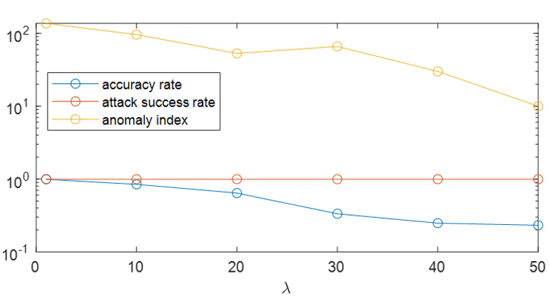
As proposed in [45], it is important to evaluate the proposed defense algorithm on the adaptive attacks where the attacker knows the defenses and tries to bypass them. In [45], an adversarial embedding attack is proposed, where the differences between the poisoned and genuine representations are minimized so that defenses based on representation distinguishing could be bypassed. To achieve this, they modify the original loss function by adding a classification accuracy based loss which reveals whether representations correspond to correct classes, i.e., poisoned or genuine. We implement the adversarial embedding attack via the Adversarial Robustness toolbox [46]. We use the same experiment setting in [45], injecting a backdoor trigger in 5% of training samples and setting their labels to their arbitrarily chosen target label . We increase the weight () for the loss of the discriminative network, that is, force the genuine and poisoned representations to be closer, so that the ability of the adversarial embedding attack to bypass our algorithm can increase. Fig. 12 shows that with the increase of the weight, the accuracy of the backdoored model decreases heavily, e.g., around 20% for and , while our algorithm can still detect the poisoned classes since the anomaly index of the poisoned class for each exceeds the threshold 3.
VI-G The selection of k
In our algorithm, we first extract the latent subspace of the training data, which is the top components from principal component analysis (PCA). The selection of can resort to several methods, such as the cross validation and cumulative percentage variance [47, 48]. In this work, we determine the number of components in , i.e., the eigenvectors, by the cumulative percentage variance (CPV) [47], which is a measure of how much variation is captured by the first components and is
| (11) |
where is the th eigenvalue describing the variation of the th component in . The number of components, a.k.a., the parameter , is selected when CPV reaches the threshold, say 95%, where the statistical variation of data is captured with noise excluded.
We also experiment with different thresholds of CPV from 95% to 99% on the GTSRB dataset and summarize the anomaly index for infected class in Table XIII. We can see that the anomaly index for different CPV are almost the same, indicating that our backdoor detection algorithm does not rely on the threshold of CPV when it exceeds 95%, since major variation is captured.
| CPV | 95% | 96% | 97% | 98% | 99% |
| Anomaly index | 35.45 | 37.52 | 36.89 | 34.51 | 35.22 |
VII Comparison with state-of-the-art
In this section, we compare our method with three state-of-the-art methods which, similar to our method, defend against backdoor attacks in neural networks by distinguishing poisoned samples from the clean ones.
VII-A Spectral signatures
Spectral signatures [15] identifies the poisoned samples by the top principals of corrupted data. Their intuition is that if the means of the authentic and poisoned representations are sufficiently well-separated relative to their variance, the correlations of the poisoned samples with the top principal component of the corrupted data via singular value decomposition are large in magnitude. Then the backdoor can be removed by excluding a fixed number of samples with large correlations. We remove 15% samples with top correlations as suggested in [15]. In this manner, Spectral signatures can remove less than 50% of the poisoned samples for ILSVARC2012 and less than 30% for GTSRB. After removing the suspicious samples and retraining the backdoored models, the repaired models still hold high Attack Success rates as shown in Table XII, which is not sufficient to mitigate the influence of the backdoor.
VII-B Activation clustering
AC [16] uses a similar strategy to Spectral signatures. It is based on the idea that the representations of the data in the infected class can be separated into two clusters, the poisoned and the authentic ones, by clustering the top principal components by K-means. They cluster each class to two groups and the one with significantly large Silhouette Score is considered to be infected since two clusters better describe this class. In their paper [16], the authors recommend to set a threshold between 0.10 and 0.15 and the class with the Silhouette Score larger than this threshold will be detected as the infected class. We use AC on the infected representations in our experiments and report the detection performance in Table VI with different thresholds (0.10, 0.11, 0.12, 0.13, 0.14, 0.15). AC can detect more than 50% infected classes when the threshold is 0.10, but it also introduces large false positive, e.g., wrongly detecting around 50% clean classes as the infected; while for larger thresholds, AC loses efficiency of detecting the infected classes. The reason AC fails lies on that the Silhouette Score of the clean and infected classes are in the same scale e.g., both ranging from 0.08 to 0.14, so that it has issues detecting the infected class by setting a threshold and determining those beyond the threshold as infected. Furthermore, we investigate its capability of identifying the genuine and poisoned samples in the infected classes in Table VII, assuming that it can first successfully detect them. We compute true positive rate (TPR) and false positive rate (FPR), in order to evaluate the performance of identifying genuine samples and poisoned samples, respectively. As summarized in Table VII, our method has larger TPR (e.g., larger than ) and FPR (e.g., as small as ) than AC (e.g., with TPR no more than and FPR around ), which implies our method exceeds the performance of AC.
VII-C SCAn
SCAn provides a strategy to distinguish the distributions of the poisoned and the authentic. It assumes that the representations of poisoned data and authentic data in the infected classes both follow Gaussian distributions with the same variance and different means. They propose an iterative algorithm to untangle the data to two groups for each class and establish a test statistic based on the likelihood ratio. The test statistic for some class exceeding the threshold indicates the high probability that the data in this class follow two Gaussian distributions mixture, which indicates this class is infected. We also evaluate this method on our infected representations. As shown in Table VI, SCAn achieves comparable infected class detect rates as our method, however, with many more clean classes identified as the infected. As shown in Table VII, SCAn can only identify around 60% poisoned samples with around 40% authentic ones identified as the poisoned. It cannot correctly cluster the authentic and poisoned data into two subgroups in our cases and cannot help repair the infected models. Besides, the running time for the dataset mentioned in Section V-C are 11.2 hours for ILSVARC2012 dataset and 550 seconds for GTSRB dataset respectively, which are much longer than our PiDAn algorithm.
VIII Conclusion
This paper has presented a novel backdoor attack detection and mitigation method by solving a coherence optimization problem. The efficacy of our method has been theoretically and empirically illustrated. On the theoretical side, we prove that the weight vector (obtained by coherence optimization formulation) has a “grouping effect” and is different for authentic data and poisoned data, which enables the detection and mitigation of backdoor attacks. At the same time, extensive experiments against three state-of-the-art backdoor schemes, including the emerging hidden trigger backdoor attack, validate the effectiveness and robustness of our method in detecting the infected classes. Our method can successfully identify more than 95% poisoned samples with less than 10% authentic samples identified as poisoned. Therefore, our method can also help mitigate the backdoor influence by correctly removing the poisoned samples from the training dataset and also maintain high classification accuracy.
Open Source
All the source code and dataset proposed will be open-sourced after the review process.
References
- [1] J. Dumford and W. Scheirer, “Backdooring convolutional neural networks via targeted weight perturbations,” in 2020 IEEE International Joint Conference on Biometrics (IJCB). IEEE, 2020, pp. 1–9.
- [2] H. Zhong, C. Liao, A. C. Squicciarini, S. Zhu, and D. Miller, “Backdoor embedding in convolutional neural network models via invisible perturbation,” in Proceedings of the Tenth ACM Conference on Data and Application Security and Privacy, 2020, pp. 97–108.
- [3] A. S. Rakin, Z. He, and D. Fan, “Tbt: Targeted neural network attack with bit trojan,” in Proceedings of the IEEE/CVF Conference on Computer Vision and Pattern Recognition (CVPR), June 2020.
- [4] S. Li, M. Xue, B. Zhao, H. Zhu, and X. Zhang, “Invisible backdoor attacks on deep neural networks via steganography and regularization,” IEEE Transactions on Dependable and Secure Computing, 2020.
- [5] Y. Yao, H. Li, H. Zheng, and B. Y. Zhao, “Latent backdoor attacks on deep neural networks,” in Proceedings of the 2019 ACM SIGSAC Conference on Computer and Communications Security, 2019, pp. 2041–2055.
- [6] E. Bagdasaryan and V. Shmatikov, “Blind backdoors in deep learning models,” arXiv preprint arXiv:2005.03823, 2020.
- [7] U. Cohen, S. Chung, D. D. Lee, and H. Sompolinsky, “Separability and geometry of object manifolds in deep neural networks,” Nature communications, vol. 11, no. 1, pp. 1–13, 2020.
- [8] P. P. Brahma, D. Wu, and Y. She, “Why deep learning works: A manifold disentanglement perspective,” IEEE transactions on neural networks and learning systems, vol. 27, no. 10, pp. 1997–2008, 2015.
- [9] E. Sarkar, Y. Alkindi, and M. Maniatakos, “Backdoor suppression in neural networks using input fuzzing and majority voting,” IEEE Design & Test, vol. 37, no. 2, pp. 103–110, 2020.
- [10] B. Wang, Y. Yao, S. Shan, H. Li, B. Viswanath, H. Zheng, and B. Y. Zhao, “Neural cleanse: Identifying and mitigating backdoor attacks in neural networks,” in 2019 IEEE Symposium on Security and Privacy (SP). IEEE, 2019, pp. 707–723.
- [11] Y. Liu, W.-C. Lee, G. Tao, S. Ma, Y. Aafer, and X. Zhang, “Abs: Scanning neural networks for back-doors by artificial brain stimulation,” in Proceedings of the 2019 ACM SIGSAC Conference on Computer and Communications Security, 2019, pp. 1265–1282.
- [12] Y. Gao, C. Xu, D. Wang, S. Chen, D. C. Ranasinghe, and S. Nepal, “Strip: A defence against trojan attacks on deep neural networks,” in Proceedings of the 35th Annual Computer Security Applications Conference, 2019, pp. 113–125.
- [13] E. Chou, F. Tramèr, and G. Pellegrino, “Sentinet: Detecting localized universal attacks against deep learning systems,” in 2020 IEEE Security and Privacy Workshops (SPW). IEEE, 2020, pp. 48–54.
- [14] D. Tang, X. Wang, H. Tang, and K. Zhang, “Demon in the variant: Statistical analysis of dnns for robust backdoor contamination detection,” in 30th USENIX Security Symposium (USENIX Security 21), 2021.
- [15] B. Tran, J. Li, and A. Madry, “Spectral signatures in backdoor attacks,” arXiv preprint arXiv:1811.00636, 2018.
- [16] B. Chen, W. Carvalho, N. Baracaldo, H. Ludwig, B. Edwards, T. Lee, I. Molloy, and B. Srivastava, “Detecting backdoor attacks on deep neural networks by activation clustering,” arXiv preprint arXiv:1811.03728, 2018.
- [17] T. Gu, K. Liu, B. Dolan-Gavitt, and S. Garg, “Badnets: Evaluating backdooring attacks on deep neural networks,” IEEE Access, vol. 7, pp. 47 230–47 244, 2019.
- [18] X. Chen, C. Liu, B. Li, K. Lu, and D. Song, “Targeted backdoor attacks on deep learning systems using data poisoning,” CoRR, vol. abs/1712.05526, 2017.
- [19] Y. Liu, X. Ma, J. Bailey, and F. Lu, “Reflection backdoor: A natural backdoor attack on deep neural networks,” arXiv preprint arXiv:2007.02343, 2020.
- [20] A. Shafahi, W. R. Huang, M. Najibi, O. Suciu, C. Studer, T. Dumitras, and T. Goldstein, “Poison frogs! targeted clean-label poisoning attacks on neural networks,” in Proceedings of the 32nd International Conference on Neural Information Processing Systems, 2018, pp. 6106–6116.
- [21] A. Saha, A. Subramanya, and H. Pirsiavash, “Hidden trigger backdoor attacks,” in Proceedings of the AAAI Conference on Artificial Intelligence, vol. 34, no. 07, 2020, pp. 11 957–11 965.
- [22] S. Kolouri, A. Saha, H. Pirsiavash, and H. Hoffmann, “Universal litmus patterns: Revealing backdoor attacks in cnns,” in Proceedings of the IEEE/CVF Conference on Computer Vision and Pattern Recognition, 2020, pp. 301–310.
- [23] X. Qiao, Y. Yang, and H. Li, “Defending neural backdoors via generative distribution modeling,” arXiv preprint arXiv:1910.04749, 2019.
- [24] A. Achille and S. Soatto, “Emergence of invariance and disentanglement in deep representations,” The Journal of Machine Learning Research, vol. 19, no. 1, pp. 1947–1980, 2018.
- [25] S. Huang, W. Peng, Z. Jia, and Z. Tu, “One-pixel signature: Characterizing cnn models for backdoor detection,” in European Conference on Computer Vision. Springer, 2020, pp. 326–341.
- [26] Z. Xiang, D. J. Miller, and G. Kesidis, “Detection of backdoors in trained classifiers without access to the training set,” IEEE Transactions on Neural Networks and Learning Systems, 2020.
- [27] ——, “A benchmark study of backdoor data poisoning defenses for deep neural network classifiers and a novel defense,” in 2019 IEEE 29th International Workshop on Machine Learning for Signal Processing (MLSP). IEEE, 2019, pp. 1–6.
- [28] W. Guo, L. Wang, X. Xing, M. Du, and D. Song, “Tabor: A highly accurate approach to inspecting and restoring trojan backdoors in ai systems,” arXiv preprint arXiv:1908.01763, 2019.
- [29] X. Huang, M. Alzantot, and M. Srivastava, “Neuroninspect: Detecting backdoors in neural networks via output explanations,” arXiv preprint arXiv:1911.07399, 2019.
- [30] H. Chen, C. Fu, J. Zhao, and F. Koushanfar, “Deepinspect: A black-box trojan detection and mitigation framework for deep neural networks.” in IJCAI, 2019, pp. 4658–4664.
- [31] W. Li, C. Zhao, and F. Gao, “Linearity evaluation and variable subset partition based hierarchical process modeling and monitoring,” IEEE Transactions on Industrial Electronics, vol. 65, no. 3, pp. 2683–2692, 2017.
- [32] L. Feng, C. Zhao, and B. Huang, “A slow independent component analysis algorithm for time series feature extraction with the concurrent consideration of high-order statistic and slowness,” Journal of Process Control, vol. 84, pp. 1–12, 2019.
- [33] Y. Qin, W.-T. Li, C. Yuen, W. Tushar, and T. Saha, “Iiot-enabled health monitoring for integrated heat pump system using mixture slow feature analysis,” IEEE Transactions on Industrial Informatics, 2021.
- [34] W. Yu, C. Zhao, and B. Huang, “Moninet with concurrent analytics of temporal and spatial information for fault detection in industrial processes,” IEEE Transactions on Cybernetics, 2021.
- [35] J. Fan, C. Zhang, and J. Zhang, “Generalized likelihood ratio statistics and wilks phenomenon,” Annals of statistics, pp. 153–193, 2001.
- [36] T. K. Moon, “The expectation-maximization algorithm,” IEEE Signal processing magazine, vol. 13, no. 6, pp. 47–60, 1996.
- [37] P. J. Rousseeuw and C. Croux, “Alternatives to the median absolute deviation,” Journal of the American Statistical association, vol. 88, no. 424, pp. 1273–1283, 1993.
- [38] K. Teknomo, “K-means clustering tutorial,” Medicine, vol. 100, no. 4, p. 3, 2006.
- [39] O. Russakovsky, J. Deng, H. Su, J. Krause, S. Satheesh, S. Ma, Z. Huang, A. Karpathy, A. Khosla, M. Bernstein et al., “Imagenet large scale visual recognition challenge,” International journal of computer vision, vol. 115, no. 3, pp. 211–252, 2015.
- [40] J. Stallkamp, M. Schlipsing, J. Salmen, and C. Igel, “Man vs. computer: Benchmarking machine learning algorithms for traffic sign recognition,” Neural networks, vol. 32, pp. 323–332, 2012.
- [41] A. Krizhevsky, I. Sutskever, and G. E. Hinton, “Imagenet classification with deep convolutional neural networks,” Advances in neural information processing systems, vol. 25, pp. 1097–1105, 2012.
- [42] C. Leys, C. Ley, O. Klein, P. Bernard, and L. Licata, “Detecting outliers: Do not use standard deviation around the mean, use absolute deviation around the median,” Journal of experimental social psychology, vol. 49, no. 4, pp. 764–766, 2013.
- [43] T. Gu, B. Dolan-Gavitt, and S. Garg, “Badnets: Identifying vulnerabilities in the machine learning model supply chain,” arXiv preprint arXiv:1708.06733, 2017.
- [44] E. Sarkar, H. Benkraouda, and M. Maniatakos, “Facehack: Triggering backdoored facial recognition systems using facial characteristics,” arXiv preprint arXiv:2006.11623, 2020.
- [45] R. Shokri et al., “Bypassing backdoor detection algorithms in deep learning,” in 2020 IEEE European Symposium on Security and Privacy (EuroS&P). IEEE, 2020, pp. 175–183.
- [46] M.-I. Nicolae, M. Sinn, M. N. Tran, B. Buesser, A. Rawat, M. Wistuba, V. Zantedeschi, N. Baracaldo, B. Chen, H. Ludwig et al., “Adversarial robustness toolbox v1. 0.0,” arXiv preprint arXiv:1807.01069, 2018.
- [47] W. Li, H. H. Yue, S. Valle-Cervantes, and S. J. Qin, “Recursive pca for adaptive process monitoring,” Journal of process control, vol. 10, no. 5, pp. 471–486, 2000.
- [48] W. Li, C. Yang, and S. E. Jabari, “Nonlinear traffic prediction as a matrix completion problem with ensemble learning,” 2021.
Appendix A Proof of Remark 3
For the optimization problem in Eq.(5), the Lagrangian function is
| (12) |
Since is the optimal solution of Eq.(5), we have
| (13) |
This gives
| (14) |
where, is the th row of and is the th element in . From Eq.(14), we further have,
| (15) |
Since and , we have
| (16) |
when data points are normalized. This completes the proof.
| Layer Type | # of Channels | Filter Size | Stride | Activation |
| Conv | 32 | 33 | 1 | ReLU |
| Conv | 32 | 33 | 1 | ReLU |
| MaxPool | 32 | 22 | 2 | – |
| Conv | 64 | 33 | 1 | ReLU |
| Conv | 64 | 33 | 1 | ReLU |
| MaxPool | 64 | 22 | 2 | – |
| Conv | 128 | 33 | 1 | ReLU |
| Conv | 128 | 33 | 1 | ReLU |
| MaxPool | 128 | 22 | 2 | – |
| FC | 512 | – | – | ReLU |
| FC | 43 | – | – | Softmax |
Appendix B Definition of flattening metric
The flattening metric is derived based on the similarity between Euclidean distance and Geodesic distance that is approximated by graph distance. By forming up a nearest neighborhood graph for all samples, the Geodesic distance between two points can be approximated by the sum of the length of edges included in the shortest path.
Let denotes the Geodesic distance between sample and , we have
| (17) |
where is the length of th edge included in the shortest path. The Euclidean distance between sample and is given by
| (18) |
Let and denote the vectors containing Geodesic distance and Euclidean distance for all pairs of points, respectively. The flattening metric is defined as
| (19) |
where and denote the normalized and , and is the number of all samples.