跳到论文正文
W Papers独立论文阅读器 arXiv:2203.09255 论文正文 计算阅读时间 · 0%
引用这篇论文根据当前论文元数据生成,正式投稿前建议核对。


License: arXiv.org perpetual non-exclusive license
arXiv:2203.09255v1 [cs.LG] 17 Mar 2022

On the Spectral Bias of Convolutional Neural Tangent and Gaussian Process Kernels

Amnon Geifman     Meirav Galun     David Jacobs    Ronen Basri Affiliation: Weizmann Institute of Science, Rehovot, Israel Affiliation: Weizmann Institute of Science, Rehovot, Israel Affiliation: Weizmann Institute of Science, Rehovot, Israel Affiliation: University of Maryland at College Park, MD, USA
Abstract

We study the properties of various over-parametrized convolutional neural architectures through their respective Gaussian process and neural tangent kernels. We prove that, with normalized multi-channel input and ReLU activation, the eigenfunctions of these kernels with the uniform measure are formed by products of spherical harmonics, defined over the channels of the different pixels. We next use hierarchical facotorizable kernels to bound their respective eigenvalues. We show that the eigenvalues decay polynomially, quantify the rate of decay, and derive measures that reflect the composition of hierarchical features in these networks. Our results provide concrete quantitative characterization of over-parameterized convolutional network architectures.

1 Introduction

Convolutional Neural Networks (CNNs) [24] have produced dramatic improvements over past machine learning approaches [23, 37, 19]. Two key properties that distinguish CNNs are their ability to encode geometric properties of the data, by incorporating multiscale analysis and invariance or equivariance. Shift invariant networks produce the same output when the input is shifted, which can be valuable, for example, in classification tasks in which objects are not well aligned. Shift equivariant networks produce shifted output when the input is shifted, and are important in image-to-image networks that, for example, denoise or segment the input [22, 25, 40]. Multiscale feature representations naturally arise in these networks through their depth.

However, we still lack a theoretical analysis of CNNs that can quantitatively predict their behavior. Our analysis builds on the Gaussian Process and Neural Tangent kernels (resp. GPK and NTK). It has been shown theoretically that massively overparameterized networks can be well approximated by a linearization about their initialization [1, 2, 15, 21]. With this linearization, neural networks become kernel regressors, with training dynamics and smoothness properties determined by the eigenfunctions and eigenvalues of their kernel, which determine their Reproducing Kernel Hilbert Space (RKHS).

A series of interesting works has derived the spectrum of NTK for fully connected networks (denoted FC-NTK). This eigen-analysis tells us which functions a network learns most rapidly, since the speed of learning an eigenfunction with gradient descent (GD) is inversely proportional to the corresponding eigenvalue. For example, it allows us to determine that FC-NTK learns low frequency components of a function faster than high frequency components, and characterize the rates at which this happens [4, 6, 5, 8, 9]. So this eigen-analysis allows us to characterize the inductive bias of over-parametrized neural networks. Convolutional GPKs and NTKs (resp. CGPKs and CNTKs) have been derived for convolutional networks [2, 32], but a characterization of their spectral bias is still missing.

In this paper we investigate the Gaussian process and neural tangent kernels associated with three deep convolutional architectures. In particular, we consider kernels associated with a shift equivariant architecture, a convnet in which the last layer is fully connected, and a convnet with a final global average pooling step. The former network is applicable to various image processing tasks. The second network is similar in architecture to AlexNet and VGG [23, 37]. The latter network resembles a residual network [19], without skip connections. All models we consider use ReLU activation. While we do not explicitly account for intermediate pooling, our work can readily be extended to handle such layers as well.

We assume our networks receive multi-channel input signals, with the channels for each pixel normalized to unit norm. Our results establish that:

  1. 1.

    The eigenfunctions of the three kernels include either products of spherical harmonics (SHs) or their shift invariant sums, with each harmonic term defined over the channels of one pixel.

  2. 2.

    The corresponding eigenvalues decay polynomially with the frequency of the eigenfunctions, at a rate that depends on the number of input channels.

  3. 3.

    The eigenvalues include a multiplicative factor that reflects the hierarchical structure of the features in the corresponding network. With the equivariant architecture, this factor is large for pixels at the center of the receptive field and small in the periphery. For the other two kernels this multiplicative factor is large for pixels close to each other and becomes very small for pixels far from each other.

Our results show that CNNs, like FC-networks, are biased toward learning low frequency functions. However, point (2) tells us that CNNs can learn high frequency functions, when these are localized in a subset of the pixels, much more rapidly than FC networks. It is important to keep in mind that we are referring to the frequency of the function the network has learned, which is a function over the space of all images; this does not refer to the power spectrum of individual images. Put differently, high frequency reflects high variability of the target function for similar input images. Interestingly, the rate of decay does not depend directly on image size or the size of the convolution filter. Point (3) tells us that CNNs learn spatially localized functions more rapidly than functions with global dependence on an entire image. This shows that CNNs can change their output significantly based on relatively small, spatially localized features; FC networks will take much longer to learn these spatially localized features. In both cases we quantify this bias.

2 Preliminaries and notations

We consider a multi-channel 1-D input signal 𝐱\mathbf{x} of length dd with ζ\zeta channels, represented by a ζ×d\zeta\times d matrix. We further set D=ζ​dD=\zeta d and refer to the columns of 𝐱\mathbf{x} as pixels, denoted 𝐱(i)∈ℝζ\mathbf{x}^{(i)}\in\mathbb{R}^{\zeta}, i∈[d]i\in[d]. We note that our results can readily be applied also to 2-D, multi-channel signals. We assume further that the entries of each pixel are normalized to unit norm, i.e., ‖(x1(i),…,xζ(i))‖=1\left\|\left(x_{1}^{(i)},...,x_{\zeta}^{(i)}\right)\right\|=1. The input space, therefore, is a Cartesian product of spheres, which we call multisphere, i.e., 𝐱∈𝕄​𝕊​(ζ,d)=𝕊ζ−1×…×𝕊ζ−1⏟d⊂𝕊D−1\mathbf{x}\in\mathbb{MS}(\zeta,d)=\underbrace{\mathbb{S}^{\zeta-1}\times...\times\mathbb{S}^{\zeta-1}}_{d}\subset\mathbb{S}^{D-1} (with radius d\sqrt{d}). We denote by si​𝐱=(xi+1,…​xd,x1,…​xi)s_{i}\mathbf{x}=(x_{i+1},...x_{d},x_{1},...x_{i}) the cyclic shift of 𝐱\mathbf{x} to the left by ii pixels.

We use multi-index notations, i.e., 𝐧=(n1,…,nd),𝐤=(k1,…,kd)∈ℕd\mathbf{n}=(n_{1},...,n_{d}),\mathbf{k}=(k_{1},...,k_{d})\in\mathbb{N}^{d} to denote vectors of polynomial orders or frequencies. ℕ\mathbb{N} denotes the natural numbers including zero, and b𝐧,λ𝐤∈ℝb_{\mathbf{n}},\lambda_{\mathbf{k}}\in\mathbb{R} are scalars that depend on vectors of indices 𝐧\mathbf{n} or 𝐤\mathbf{k}. We denote monomials by 𝐭𝐧=t1n1​t2n2⋅…⋅tdnd\mathbf{t}^{\mathbf{n}}=t_{1}^{n_{1}}t_{2}^{n_{2}}\cdot\ldots\cdot t_{d}^{n_{d}} with 𝐭∈ℝd\mathbf{t}\in\mathbb{R}^{d}, and allow also for a scalar exponent, i.e., 𝐭n=(t1⋅…⋅td)n\mathbf{t}^{n}=(t_{1}\cdot...\cdot t_{d})^{n}. For 𝐮,𝐯∈ℝd\mathbf{u},\mathbf{v}\in\mathbb{R}^{d} we say that 𝐮≥𝐯\mathbf{u}\geq\mathbf{v} if ui≥viu_{i}\geq v_{i} for all i∈[d]i\in[d]. Therefore, the power series ∑𝐧≥𝟎b𝐧​𝐭𝐧\sum_{\mathbf{n}\geq\mathbf{0}}b_{\mathbf{n}}\mathbf{t}^{\mathbf{n}} should read ∑n1≥0,n2≥0,…bn1,n2,…​t1n1​t2n2​…\sum_{n_{1}\geq 0,n_{2}\geq 0,...}b_{n_{1},n_{2},...}t_{1}^{n_{1}}t_{2}^{n_{2}}...

We denote the uniform distribution in a domain Ω\Omega by Unif⁡(Ω)\mathrm{Unif}(\Omega). We write f⁡(x)∼g⁡(x)f(x)\sim g(x) when limx→∞f⁡(x)/g⁡(x)=1\lim_{x\rightarrow\infty}f(x)/g(x)=1. Throughout the paper we assume all kernels are differentiable at zero infinitely many times and their power series converge in the hypercube [−1,1]d[-1,1]^{d}. Our theorems and lemmas are proved in the appendix.

2.1 The network model

We consider convolutional neural network architectures (Figure 1) of the following form. Given a multi-channel 1-D input signal 𝐱∈𝕄​𝕊​(ζ,d)\mathbf{x}\in\mathbb{MS}(\zeta,d) arranged in a ζ×d\zeta\times d matrix, we use a shift equivariant backbone and three heads to produce scalar features. The network, defined in Table 1, begins with a 1×11\times 1 convolution layer, followed by L−1≥1L-1\geq 1 stride-1 convolutional layers with filters of size qq, producing at each layer the same number of feature channels mm in each of the dd locations.

Refer to caption
Figure 1: Network architecture. An input signal 𝐱∈ℝζ×d\mathbf{x}\in\mathbb{R}^{\zeta\times d} (left column) is fed into an equivariant backbone (dashed box), producing mm feature channels for each pixel, first using 1×11\times 1 convolution, followed by L−1L-1 convolution layers with filters of size qq (marked by blueish pyramids), interleaved with ReLU activation. The backbone is followed by one of three heads, fEqf^{\mathrm{Eq}}, fTrf^{\mathrm{Tr}} and fGAPf^{\mathrm{GAP}}.
Table 1: Network model.

1. 𝐟(1)​(𝐱,θ)=σ⁡(W(1)​𝐱)\mathbf{f}^{(1)}(\mathbf{x},\theta)=\sigma\left(W^{(1)}\mathbf{x}\right). 2. 𝐟i(l)(𝐱,θ)=σ(cσm​q(∑j=1mW:,i,j(l)∗𝐟j(l−1)(𝐱,θ)))\mathbf{f}_{i}^{(l)}(\mathbf{x},\theta)=\sigma\left(\sqrt{\frac{c_{\sigma}}{mq}}\left(\sum_{j=1}^{m}W_{:,i,j}^{(l)}*\mathbf{f}_{j}^{(l-1)}(\mathbf{x},\theta)\right)\right), 3. with l∈{2,…,L}l\in\{2,\ldots,L\}, i∈[m]i\in[m], and three heads: (a) fEq(𝐱,θ)=⟨𝐰Eq,𝐟:,1(L)(𝐱,θ)⟩f^{\mathrm{Eq}}(\mathbf{x},\theta)=\langle\mathbf{w}^{\mathrm{Eq}},\mathbf{f}^{(L)}_{:,1}(\mathbf{x},\theta)\rangle. (b) fTr​(𝐱,θ)=1d​⟨WTr,𝐟(L)​(𝐱,θ)⟩f^{\mathrm{Tr}}(\mathbf{x},\theta)=\frac{1}{\sqrt{d}}\langle W^{\mathrm{Tr}},\mathbf{f}^{(L)}(\mathbf{x},\theta)\rangle. (c) fGAP​(𝐱,θ)=1d​𝐰GAP​𝐟(L)​(𝐱,θ)​𝟏f^{\mathrm{GAP}}(\mathbf{x},\theta)=\frac{1}{d}\mathbf{w}^{\mathrm{GAP}}\mathbf{f}^{(L)}(\mathbf{x},\theta)\mathbf{1}. Here 𝐟(l)∈ℝm×d\mathbf{f}^{(l)}\in\mathbb{R}^{m\times d} (ł∈[L]\l\in[L]); θ=(W(1),…,W(L),WTr,𝐰GAP,𝐰Eq)\theta=\left(W^{(1)},...,W^{(L)},W^{\mathrm{Tr}},\mathbf{w}^{\mathrm{GAP}},\mathbf{w}^{\mathrm{Eq}}\right) are learnable parameters initialized with 𝒩⁡(0,I){\cal N}(0,I). W(1)∈ℝm×ζW^{(1)}\in\mathbb{R}^{m\times\zeta}, W(l)∈ℝq×m×mW^{(l)}\in\mathbb{R}^{q\times m\times m} (i.e., W:,i,j(l)W_{:,i,j}^{(l)} is a filter of size qq), WTr∈ℝm×dW^{\mathrm{Tr}}\in\mathbb{R}^{m\times d} (⟨⋅,⋅⟩\langle\cdot,\cdot\rangle denotes the standard inner product between matrices), 𝐰Eq,𝐰GAP∈ℝ1×m\mathbf{w}^{\mathrm{Eq}},\mathbf{w}^{\mathrm{GAP}}\in\mathbb{R}^{1\times m} and 𝟏=(1,…,1)T∈ℝd\mathbf{1}=(1,...,1)^{T}\in\mathbb{R}^{d}. ’*’ denotes cyclic convolution; σ\sigma is the ReLU function, and for ReLU, cσ=1/(𝔼z∼𝒩⁡(0,1)​[σ​(z)2])=2c_{\sigma}=1/\left(\mathbb{E}_{z\sim\mathcal{N}(0,1)}[\sigma(z)^{2}]\right)=2.

The fEqf^{\mathrm{Eq}} head produces one scalar entry for the shift equivariant network (i.e., the tuple (fEq​(𝐱,⋅),…,fEq​(sd−1​𝐱,⋅))(f^{\mathrm{Eq}}(\mathbf{x},\cdot),...,f^{\mathrm{Eq}}(s_{d-1}\mathbf{x},\cdot)) produces the shift-equivariant output); fTrf^{\mathrm{Tr}} corresponds to applying a fully connected layer at the top layer, and fGAPf^{\mathrm{GAP}} corresponds to applying global average pooling, resulting in a shift invariant network. With each of the heads, the network parameters are trained for regression with the mean square error (MSE) loss.

2.2 Derivation of CGPK and CNTK

Previous work showed that in the limit of infinite width and with small initialization, massively over-parameterized neural networks become kernel regressors with a family of kernels called neural tangent kernels [21]. Let f⁡(𝐱,θ)f(\mathbf{x},\theta) denote a network, then for a pair of inputs 𝐱i,𝐱j\mathbf{x}_{i},\mathbf{x}_{j}, the corresponding NTK is defined as 𝒌−(𝐱i,𝐱j)=𝔼θ∼𝒫⟨∂f⁡(𝐱i,θ)∂θ,∂f⁡(𝐱j,θ)∂θ⟩\mathrlap{{}^{-}}\boldsymbol{k}(\mathbf{x}_{i},\mathbf{x}_{j})=\mathbb{E}_{\theta\sim\mathcal{P}}\left<\frac{\partial f(\mathbf{x}_{i},\theta)}{\partial\theta},\frac{\partial f(\mathbf{x}_{j},\theta)}{\partial\theta}\right>. A related kernel, called the Gaussian process (or random feature) kernel, is obtained if the weights are kept in their initial random values, and only the last layer of the network is optimized in training [12].

[2] derived expressions for CNTK and CGPK for convolutional networks. The formulas in Table 3 adapt these expressions to our convolutional architectures and to multisphere inputs. We note that with general input in ℝD\mathbb{R}^{D} additional normalization steps are needed. We refer the reader to [2] for the full derivation.

Table 2: CGPK and CNTK formulas.

Given 𝐱,𝐳∈𝕄​𝕊​(ζ,d)\mathbf{x},\mathbf{z}\in\mathbb{MS}(\zeta,d), we denote respectively by XX and ZZ their ζ×d\zeta\times d matrix representations. Let Σ(0)​(𝐱,𝐳)=Θ(0)​(𝐱,𝐳)=XT​Z\Sigma^{(0)}(\mathbf{x},\mathbf{z})=\Theta^{(0)}(\mathbf{x},\mathbf{z})=X^{T}Z. For l∈[L]l\in[L] and for i,j∈[d]i,j\in[d], 1. Σi,j(1)​(𝐱,𝐳)=κ1​(Σi,j(0)​(𝐱,𝐳))\Sigma_{i,j}^{(1)}(\mathbf{x},\mathbf{z})=\kappa_{1}\left(\Sigma_{i,j}^{(0)}(\mathbf{x},\mathbf{z})\right). 2. Σ˙i,j(1)​(𝐱,𝐳)=κ0​(Σi,j(0)​(𝐱,𝐳))\dot{\Sigma}_{i,j}^{(1)}(\mathbf{x},\mathbf{z})=\kappa_{0}\left(\Sigma_{i,j}^{(0)}(\mathbf{x},\mathbf{z})\right). 3. Θi,j(l)(𝐱,𝐳)=12​q∑r=0q−1[Σ˙~i+r,j+r(l)(𝐱,𝐳)Θ~i+r,j+r(l−1)(𝐱,𝐳)+\Theta_{i,j}^{(l)}(\mathbf{x},\mathbf{z})=\frac{1}{2q}\sum_{r=0}^{q-1}\left[\tilde{\dot{\Sigma}}_{i+r,j+r}^{(l)}(\mathbf{x},\mathbf{z})\tilde{\Theta}_{i+r,j+r}^{(l-1)}(\mathbf{x},\mathbf{z})+\right.
Σ~i+r,j+r(l)(𝐱,𝐳)]~~~~~~~~~~~~~~~~~~~~~~~~~~~~~~~~~~~~~~~~~~~~~~~~~~\left.\tilde{\Sigma}_{i+r,j+r}^{(l)}(\mathbf{x},\mathbf{z})\right].
4. Σi,j(l+1)​(𝐱,𝐳)=κ1​(1q​∑r=0q−1Σ~i+r,j+r(l)​(𝐱,𝐳))\Sigma_{i,j}^{(l+1)}(\mathbf{x},\mathbf{z})=\kappa_{1}\left(\frac{1}{q}\sum_{r=0}^{q-1}\tilde{\Sigma}_{i+r,j+r}^{(l)}(\mathbf{x},\mathbf{z})\right). 5. Σ˙i,j(l+1)​(𝐱,𝐳)=κ0​(1q​∑r=0q−1Σ~i+r,j+r(l)​(𝐱,𝐳))\dot{\Sigma}_{i,j}^{(l+1)}(\mathbf{x},\mathbf{z})=\kappa_{0}\left(\frac{1}{q}\sum_{r=0}^{q-1}\tilde{\Sigma}_{i+r,j+r}^{(l)}(\mathbf{x},\mathbf{z})\right),
where we denote by Σ~\tilde{\Sigma}, Σ˙~\tilde{\dot{\Sigma}}, and Θ~\tilde{\Theta} respectively Σ\Sigma, Σ˙\dot{\Sigma} and Θ\Theta whose rows and columns are extended with circular padding. Additionally, with ReLU activation 1. κ0​(u)=π−arccos⁡(u)π\kappa_{0}(u)=\frac{\pi-\arccos(u)}{\pi}. 2. κ1​(u)=(π−arccos⁡(u))​u+1−u2π,u∈[−1,1]\kappa_{1}(u)=\frac{(\pi-\arccos(u))u+\sqrt{1-u^{2}}}{\pi},~~u\in[-1,1].

Table 3: Kernel heads.

1. CGPK-EqNet (corresponds to fEqf^{\mathrm{Eq}}): Σ1,1(L)​(𝐱,𝐳)\Sigma_{1,1}^{(L)}(\mathbf{x},\mathbf{z}). 2. CGPK (corresponds to fTrf^{\mathrm{Tr}}): 1d​∑i=1dΣi,i(L)​(𝐱,𝐳)\frac{1}{d}\sum_{i=1}^{d}\Sigma_{i,i}^{(L)}(\mathbf{x},\mathbf{z}). 3. CGPK-GAP (corresponds to fGAPf^{\mathrm{GAP}}): 1d2​∑i=1d∑j=1dΣi,j(L)​(𝐱,𝐳)\frac{1}{d^{2}}\sum_{i=1}^{d}\sum_{j=1}^{d}\Sigma_{i,j}^{(L)}(\mathbf{x},\mathbf{z}). 4. CNTK-EqNet (corresponds to fEqf^{\mathrm{Eq}}): Θ1,1(L)​(𝐱,𝐳)\Theta_{1,1}^{(L)}(\mathbf{x},\mathbf{z}). 5. CNTK (corresponds to fTrf^{\mathrm{Tr}}): 1d​∑i=1dΘi,i(L)​(𝐱,𝐳)\frac{1}{d}\sum_{i=1}^{d}\Theta_{i,i}^{(L)}(\mathbf{x},\mathbf{z}). 6. CNTK-GAP (corresponds to fGAPf^{\mathrm{GAP}}): 1d2​∑i=1d∑j=1dΘi,j(L)​(𝐱,𝐳)\frac{1}{d^{2}}\sum_{i=1}^{d}\sum_{j=1}^{d}\Theta_{i,j}^{(L)}(\mathbf{x},\mathbf{z}).

Note that for a pair of inputs 𝐱,𝐳\mathbf{x},\mathbf{z}, this definition produces two matrices of kernels, Σi,j(L)​(𝐱,𝐳)\Sigma^{(L)}_{i,j}(\mathbf{x},\mathbf{z}) and Θi,j(L)​(𝐱,𝐳)\Theta^{(L)}_{i,j}(\mathbf{x},\mathbf{z}), i,j∈[d]i,j\in[d], and that Σi,j(L)​(𝐱,𝐳)=Σ1,1(L)​(si−1​𝐱,sj−1​𝐳)\Sigma_{i,j}^{(L)}(\mathbf{x},\mathbf{z})=\Sigma_{1,1}^{(L)}(s_{i-1}\mathbf{x},s_{j-1}\mathbf{z}) (and similarly for Θ\Theta). With these definitions, we produce six different kernels in Table 3–these describe three different architectures for each of the Gaussian process neural tangent kernels.

Below we refer to these six kernels as CGPKs and CNTKs. Note that CGPK-EqNet and CNTK-EqNet produces a single output, corresponding to the first output of the equivariant network. The tuple (𝒌−(s0𝐱,s0𝐳),…,𝒌−(sd−1𝐱,sd−1𝐳))∈ℝd\left(\mathrlap{{}^{-}}\boldsymbol{k}(s_{0}\mathbf{x},s_{0}\mathbf{z}),...,\mathrlap{{}^{-}}\boldsymbol{k}(s_{d-1}\mathbf{x},s_{d-1}\mathbf{z})\right)\in\mathbb{R}^{d} (with −𝒌\mathrlap{{}^{-}}\boldsymbol{k} either CGPK-EqNet or CNTK-EqNet) produces the full response of the equivariant network.

3 The RKHS of CGPKs and CNTKs

Our objective is to derive the spectrum of Gaussian process and neural tangent kernels associated with convolutional networks. We do so by forming bounds using products of kernels that apply to individual pixels and are composed hierarchically. We proceed below as follows. We first prove general results for kernels that are functions of inner products between pixels (Sec. 3.1). We next consider factorizable kernels and derive their spectrum (Sec. 3.2). Then, in Sec. 3.3, we refine our expressions to account for hierarchical kernels. We finally use these derivations in Sec. 3.4 and 3.5 to prove bounds for all six kernels.

3.1 Multi-dot product kernels

It can be readily shown that CNTK and CGPK associated with the shift equivariant network are functions of dot products of corresponding pixels. We refer to such kernels as multi-dot product and prove in Appendix A several results regarding their spectral properties, which we briefly summarize here.

We call a kernel 𝒌−(𝐱,𝐳):𝕄𝕊(ζ,d)×𝕄𝕊(ζ,d)\mathrlap{{}^{-}}\boldsymbol{k}(\mathbf{x},\mathbf{z}):\mathbb{MS}(\zeta,d)\times\mathbb{MS}(\zeta,d) →ℝ\rightarrow\mathbb{R} multi-dot product if 𝒌−(𝐱,𝐳)=𝒌−(𝐭)\mathrlap{{}^{-}}\boldsymbol{k}(\mathbf{x},\mathbf{z})=\mathrlap{{}^{-}}\boldsymbol{k}(\mathbf{t}), where 𝐭=(⟨𝐱(1),𝐳(1)⟩,..,⟨𝐱(d),𝐳(d)⟩)∈[−1,1]d\mathbf{t}=\left(\langle\mathbf{x}^{(1)},\mathbf{z}^{(1)}\rangle,..,\langle\mathbf{x}^{({{d}})},\mathbf{z}^{({{d}})}\rangle\right)\in[-1,1]^{d}. (Note the overload of notation, which should be clear by context.) Multi-dot product kernels can be written via Mercer’s decomposition as

𝒌−(𝐱,𝐳)=∑𝐤,𝐣λ𝐤Y𝐤,𝐣(𝐱)Y𝐤,𝐣(𝐳),\displaystyle\mathrlap{{}^{-}}\boldsymbol{k}(\mathbf{x},\mathbf{z})=\sum_{\mathbf{k},\mathbf{j}}\lambda_{\mathbf{k}}Y_{\mathbf{k},\mathbf{j}}(\mathbf{x})Y_{\mathbf{k},\mathbf{j}}(\mathbf{z}), (1)

where Y𝐤,𝐣​(𝐱)Y_{\mathbf{k},\mathbf{j}}(\mathbf{x}) (𝐤,𝐣∈ℕd\mathbf{k},\mathbf{j}\in\mathbb{N}^{d}), the eigenfunctions of −𝒌\mathrlap{{}^{-}}\boldsymbol{k}, are products of spherical harmonics in 𝕊ζ−1\mathbb{S}^{\zeta-1}, ∏r=idYki​ji​(𝐱(i))\prod_{r=i}^{d}Y_{k_{i}j_{i}}\left(\mathbf{x}^{(i)}\right), with ki≥0k_{i}\geq 0, ji∈[N⁡(ζ,ki)]j_{i}\in[N(\zeta,k_{i})], and N⁡(ζ,ki)N(\zeta,k_{i}) denotes the number of harmonics of frequency kik_{i} in 𝕊ζ−1\mathbb{S}^{\zeta-1}. Such products are harmonic polynomials in 𝕊D−1\mathbb{S}^{D-1}. With ζ=2\zeta=2, these are products of Fourier series in a multi-dimensional torus. The eigenvalues λ𝐤\lambda_{\mathbf{k}} depend on the vector of frequencies, 𝐤\mathbf{k}, and are independent of the phases 𝐣\mathbf{j}. We note that a multi-dot product kernel is universal for 𝕄​𝕊​(ζ,d)\mathbb{MS}(\zeta,d) if all its eigenvalues are strictly positive. Non-universal kernels are obtained, e.g., when the eigenfunctions involve pixels outside of the receptive field of the respective network, in which case these eigenfunctions lie in the null space of the kernel.

Below we consider multi-dot product kernels that can be expressed using a multivariate power series of the form

𝒌−(𝐭)=∑𝐧≥𝟎b𝐧𝐭𝐧=∑𝐧≥𝟎b𝐧∏i=1d⟨𝐱(i),𝐳(i)⟩ni.\displaystyle\mathrlap{{}^{-}}\boldsymbol{k}(\mathbf{t})=\sum_{\mathbf{n}\geq\mathbf{0}}b_{\mathbf{n}}\mathbf{t}^{\mathbf{n}}=\sum_{\mathbf{n}\geq\mathbf{0}}b_{\mathbf{n}}\prod_{i=1}^{d}\langle\mathbf{x}^{(i)},\mathbf{z}^{(i)}\rangle^{n_{i}}. (2)

with b𝐧≥0b_{\mathbf{n}}\geq 0 for all 𝐧≥𝟎\mathbf{n}\geq\mathbf{0}. Indeed, it can be readily shown that all our CGPKs and CNTKs are positive semidefinite (PSD) and their power series coefficients are non-negative; the kernels are obtained from the univariate PSD κ0\kappa_{0} and κ1\kappa_{1} (defined in Table 3), whose coefficients are non-negative by sequences of multiplication, addition and composition, resulting in PSD kernels with non-negative coefficients.

It is possible to calculate the eigenvalues of multi-dot product kernels from their power series coefficients. This is established in the following lemma, which extends a result by [3] to multi-dot product kernels.

Lemma 3.1.

Let −𝐤\mathrlap{{}^{-}}\boldsymbol{k} be a multi-dot product kernel with the power series given in (2), where 𝐱(i),𝐳(i)∈𝕊ζ−1\mathbf{x}^{(i)},\mathbf{z}^{(i)}\in\mathbb{S}^{\zeta-1} respectively are pixels in 𝐱,𝐳\mathbf{x},\mathbf{z}. Then, the eigenvalues λ𝐤(𝐤−)\lambda_{\mathbf{k}}(\mathrlap{{}^{-}}\boldsymbol{k}) of −𝐤\mathrlap{{}^{-}}\boldsymbol{k} are given by

λ𝐤(𝒌−)=|𝕊ζ−2|d∑𝐬≥0b𝐤+2​𝐬∏i=1dλki(tki+2​si),\displaystyle\lambda_{\mathbf{k}}(\mathrlap{{}^{-}}\boldsymbol{k})=\left|\mathbb{S}^{\zeta-2}\right|^{d}\sum_{\mathbf{s}\geq 0}b_{\mathbf{k}+2\mathbf{s}}\prod_{i=1}^{{d}}\lambda_{k_{i}}(t^{k_{i}+2s_{i}}),

where |𝕊ζ−2||\mathbb{S}^{\zeta-2}| is the surface area of 𝕊ζ−2\mathbb{S}^{\zeta-2}, and λk​(tn)\lambda_{k}(t^{n}) is the kk’th eigenvalue of tnt^{n}, given by

λk​(tn)=n!(n−k)!​2k+1​Γ⁡(ζ−12)​Γ​(n−k+12)Γ⁡(n−k+ζ2)\displaystyle\lambda_{k}(t^{n})=\frac{n!}{(n-k)!2^{k+1}}\frac{\Gamma\left(\frac{\zeta-1}{2}\right)\Gamma\left(\frac{n-k+1}{2}\right)}{\Gamma\left(\frac{n-k+\zeta}{2}\right)}

if n−kn-k is even and non-negative, while λk​(tn)=0\lambda_{k}(t^{n})=0 otherwise, and Γ\Gamma is the Gamma function.

3.2 Factorizable Kernels

Next, we consider multivariate kernels that factor into products of dot product kernels,

𝒌−(𝐱,𝐳)=∏i=1d𝒌i−(⟨𝐱(i),𝐳(i)⟩).\displaystyle\mathrlap{{}^{-}}\boldsymbol{k}(\mathbf{x},\mathbf{z})=\prod_{i=1}^{d}\mathrlap{{}^{-}}\boldsymbol{k}_{i}(\langle\mathbf{x}^{(i)},\mathbf{z}^{(i)}\rangle).

The power series of −𝒌\mathrlap{{}^{-}}\boldsymbol{k} can be written as 𝒌−(𝐭)=∏i=1d(∑n=0∞bn(i)tin)\mathrlap{{}^{-}}\boldsymbol{k}(\mathbf{t})=\prod_{i=1}^{d}\left(\sum_{n=0}^{\infty}b_{n}^{(i)}t_{i}^{n}\right). Their eigenvalues satisfy λ𝐤(𝒌−)=∏i=1dλki(𝒌i−)\lambda_{\mathbf{k}}(\mathrlap{{}^{-}}\boldsymbol{k})=\prod_{i=1}^{d}\lambda_{k_{i}}(\mathrlap{{}^{-}}\boldsymbol{k}_{i}) and can be calculated using Lemma 3.1. Below we are interested specifically in kernels whose power series decay polynomially with frequency. The next theorem shows that for such kernels, the eigenvalues too decay polynomially and derives their exact decay rate. For the theorem we further use the concept of a receptive field, which captures for a multivariate kernel the subset of variables it depends on. That is, the receptive field ℛ⊆[d]\mathcal{R}\subseteq[d] is the set of indices ii for which there exists 𝐧=(…,ni,…)\mathbf{n}=(...,n_{i},...) with ni≥1n_{i}\geq 1 and b𝐧≠0b_{\mathbf{n}}\neq 0. This condition ensures that there exists a term in the power series expansion that depends on pixel ii.

Theorem 3.2.

Let −𝐤\mathrlap{{}^{-}}\boldsymbol{k} be a factorizable multi-dot product kernel with inputs 𝐱,𝐳∈𝕄​𝕊​(ζ,d)\mathbf{x},\mathbf{z}\in\mathbb{MS}(\zeta,d), and let ℛ⊆[d]\mathcal{R}\subseteq[d] denote its receptive field. Suppose that −𝐤\mathrlap{{}^{-}}\boldsymbol{k} can be written as a multivariate power series, 𝐤−(𝐭)=∑𝐧≥0b𝐧𝐭𝐧\mathrlap{{}^{-}}\boldsymbol{k}(\mathbf{t})=\sum_{\mathbf{n}\geq 0}b_{\mathbf{n}}\mathbf{t}^{\mathbf{n}} with

b𝐧∼c​∏i∈ℛ,ni>0ni−ν.\displaystyle b_{\mathbf{n}}\sim c\prod_{i\in\mathcal{R},\,n_{i}>0}n_{i}^{-\nu}.

with constants c>0c>0, non-integer ν>1\nu>1, and b𝐧=0b_{\mathbf{n}}=0 if ni>0n_{i}>0 for any i∉ℛi\not\in\mathcal{R}. Then the eigenfunctions of −𝐤\mathrlap{{}^{-}}\boldsymbol{k} w.r.t the uniform measure are the SH-products. Moreover, let 𝐤∈ℕd\mathbf{k}\in\mathbb{N}^{d} be a vector of frequencies. Then, the eigenvalues λ𝐤(𝐤−)\lambda_{\mathbf{k}}(\mathrlap{{}^{-}}\boldsymbol{k}) satisfy

λ𝐤∼c~​∏i∈ℛ,ki>0ki−(ζ+2​ν−3).\displaystyle\lambda_{\mathbf{k}}\sim\tilde{c}\prod_{i\in\mathcal{R},\,k_{i}>0}k_{i}^{-(\zeta+2\nu-3)}.

Finally, λ𝐤=0\lambda_{\mathbf{k}}=0 if ki>0k_{i}>0 for any i∉ℛi\not\in\mathcal{R}.

The theorem above improves over previous results by [3, 35] in various ways. Specifically, these authors considered only dot product kernels (i.e., d=1d=1) and bounded the decay of their eigenvalues by a non-tight upper bound. Here we provide tight upper and lower bounds, which are identical up to a constant factor, for any d≥1d\geq 1.

3.3 Positional bias of eigenvalues

CNNs process signals by producing a hierarchy of learned features that emerge via repeated convolutions, interleaved with non-linear activations. It is natural to ask, therefore, to what extent this hierarchy is reflected in the RKHS of the CGPKs and CNTKs. To answer this question we consider kernels formed by hierarchical composition of kernels. We are further interested in such kernels that are both factorizable and whose power series decay polynomially. For such kernels we prove that their eigenvalues are larger for eigenfunctions that depend on pixels near the center of their receptive field and smaller for eigenfunctions that depend only on peripheral pixels. This in turn will allow us to derive similar bounds for the kernels associated with the equivariant network. For the trace and GAP kernels this will reveal bias to eigenfunctions that depend on nearby pixels, compared to those that depend only on more distant pixels.

Definition 3.3.

A kernel 𝒌(L)−:[−1,1]d→ℝ\mathrlap{{}^{-}}\boldsymbol{k}^{(L)}:[-1,1]^{d}\rightarrow\mathbb{R} is called (stride-1) hierarchical of depth L>1L>1 and filter size qq if there exists a sequence of kernels −𝒌(1),…,−𝒌(L)\mathrlap{{}^{-}}\boldsymbol{k}^{(1)},...,\mathrlap{{}^{-}}\boldsymbol{k}^{(L)} such that 𝒌(l)−(𝐭)=f(l)(𝒌(l−1)−(s0𝐭),…,𝒌(l−1)−(sq−1𝐭))\mathrlap{{}^{-}}\boldsymbol{k}^{(l)}(\mathbf{t})=f^{(l)}\left(\mathrlap{{}^{-}}\boldsymbol{k}^{(l-1)}(s_{0}\mathbf{t}),...,\mathrlap{{}^{-}}\boldsymbol{k}^{(l-1)}(s_{q-1}\mathbf{t})\right) with f(l):ℝq→ℝf^{(l)}:\mathbb{R}^{q}\rightarrow\mathbb{R} and 𝒌(1)−(𝐭)=f(1)(t1)\mathrlap{{}^{-}}\boldsymbol{k}^{(1)}(\mathbf{t})=f^{(1)}(t_{1}), t1∈[−1,1]t_{1}\in[-1,1].

Similar to feed-forward networks, hierarchical kernels induce a tree structure in which the leaf nodes represent the variables t1,…,tdt_{1},...,t_{d} and nodes represent function applications f(l)f^{(l)}. Each variable may be connected by multiple paths to the root node, which corresponds to the final kernel −𝒌(L)\mathrlap{{}^{-}}\boldsymbol{k}^{(L)}. The number of paths from a node tit_{i} to the root, denoted pi(L)p_{i}^{(L)}, plays an important role in the magnitude of the eigenvalues. In the next theorem we bound both the power series coefficients and the eigenvalues of hierarchical kernels, showing that the bounds depend on the number of paths in the hierarchical tree, which in turn is determined by the position of the pixel within the receptive field.

Theorem 3.4.

Let −𝐤(L)=∑𝐧≥0b𝐧𝐭𝐧\mathrlap{{}^{-}}\boldsymbol{k}^{(L)}=\sum_{\mathbf{n}\geq 0}b_{\mathbf{n}}\mathbf{t}^{\mathbf{n}} be hierarchical and factorizable of depth L>1L>1 with filter size qq, so that b𝐧=c​∏i=1,ni>0dni−νb_{\mathbf{n}}=c\prod_{i=1,n_{i}>0}^{d}n_{i}^{-\nu} for non-integer ν>1\nu>1. Then there exists a scalar A>1A>1 such that:

  1. 1.

    The power series coefficients of −𝒌(L)\mathrlap{{}^{-}}\boldsymbol{k}^{(L)} satisfy

    b𝐧≥cL​∏i=1ni>0dAmin⁡(pi(L),ni)​ni−ν.\displaystyle b_{\mathbf{n}}\geq c_{L}\prod_{\begin{subarray}{c}i=1\\ n_{i}>0\end{subarray}}^{d}{A}^{\min(p_{i}^{(L)},n_{i})}n_{i}^{-\nu}.
  2. 2.

    The eigenvalues λ𝐤(𝒌(L)−)\lambda_{\mathbf{k}}(\mathrlap{{}^{-}}\boldsymbol{k}^{(L)}) satisfy

    λ𝐤≥c~L​∏i=1ki>0dAmin⁡(pi(L),ki)​ki−(ζ+2​ν−3)\displaystyle\lambda_{\mathbf{k}}\geq\tilde{c}_{L}\prod_{\begin{subarray}{c}i=1\\ k_{i}>0\end{subarray}}^{d}{A}^{\min(p_{i}^{(L)},k_{i})}k_{i}^{-(\zeta+2\nu-3)}

where cL,c~Lc_{L},\tilde{c}_{L} are constants that depends on LL, and pi(L)p^{(L)}_{i} denotes the number of paths from pixel ii to the output of −𝐤(L)\mathrlap{{}^{-}}\boldsymbol{k}^{(L)}.

The proof exploits relations between hierarchical stride-1 and stride-q kernels and relies on recursively combining power series, which are shown to maintain their polynomial decay. We note that although the number of paths can grow rapidly with depth, the kernels we consider are normalized so that they always produce values in [−1,1][-1,1]. As a result, both the power series coefficients and the eigenvalues are bounded in [0,1][0,1]. This normalization is reflected in the magnitudes of cLc_{L} and c~L\tilde{c}_{L}.

In fact, for a hierarchical, stride-1 kernel of depth LL, the (normalized) number of paths pi(L)p_{i}^{(L)} of a pixel, 𝐱(i)\mathbf{x}^{(i)}, decays exponentially with its distance from the center of the receptive field, |i−ic||i-i_{c}|. The number of paths is determined by convolving a rectangular function of width qq, the size of the convolution filter, (i.e., r⁡(x)=1/qr(x)=1/q if 0≤x≤q0\leq x\leq q and 0 otherwise) with itself LL times. Note that such a repeated convolution is equal to the density function obtained by summing LL random variables distributed uniformly, resulting in the Irwin–Hall distribution, whose support is stretched by the size of the convolution filter qq. With sufficiently large LL, using the central limit theorem and assuming the number of pixels dd is greater than the receptive field size, the number of paths pi(L)p_{i}^{(L)} approaches a Gaussian centered at the central pixel with variance Vq,L≈L​q2/12V_{q,L}\approx Lq^{2}/12, i.e., pi(L)∝exp(−(i−ic)2/(2Vq,L))p_{i}^{(L)}\propto\exp(-(i-i_{c})^{2}/(2V_{q,L})) [26]. Roughly speaking, we can conclude that the position of a pixel within the receptive field can have an exponential effect on both the power series coefficients and the eigenvalues of the kernel.

Note that in the analysis above we assumed that the number of pixels dd is larger than the receptive field size. With a receptive field of size dd and cyclic convolutions, the number of paths from all pixels approaches a constant as LL grows. In practice, real CNNs use zero padding, which effectively ensures that dd is always larger than the receptive field.

3.4 Kernels associated with the equivariant network

The following theorem characterizes the spectrums of CGPK-EqNet and CNTK-EqNet, by proving lower and upper bounds on both their power series coefficients as well as their eigenvalues.

Theorem 3.5.

Let −𝐤(L)\mathrlap{{}^{-}}\boldsymbol{k}^{(L)} denote either CGPK-EqNet or CNTK-EqNet of depth LL whose input includes ζ\zeta channels, with receptive field ℛ\mathcal{R} and with ReLU activation. Then,

  1. 1.

    −𝒌(L)\mathrlap{{}^{-}}\boldsymbol{k}^{(L)} can be written as a power series, 𝒌(L)−(𝐭)=∑𝐧≥0b𝐧𝐭𝐧\mathrlap{{}^{-}}\boldsymbol{k}^{(L)}(\mathbf{t})=\sum_{\mathbf{n}\geq 0}b_{\mathbf{n}}\mathbf{t}^{\mathbf{n}} with

    c1​∏i∈ℛ,ni>0A~min⁡(pi(L),ni)​ni−νa≤b𝐧≤c2​∏i∈ℛ,ni>0ni−νb,\displaystyle c_{1}\prod_{i\in\mathcal{R},n_{i}>0}\tilde{A}^{\min(p_{i}^{(L)},n_{i})}n_{i}^{-\nu_{a}}\leq b_{\mathbf{n}}\leq c_{2}\prod_{i\in\mathcal{R},n_{i}>0}n_{i}^{-\nu_{b}},
  2. 2.

    The eigenvalues of −𝒌(L)\mathrlap{{}^{-}}\boldsymbol{k}^{(L)} are bounded by

    c3​∏i∈ℛki>0A~min⁡(pi(L),ki)​ki−(ζ+2​νa−3)≤λ𝐤≤c4​∏i∈ℛki>0ki−(ζ+2​νb−3),\displaystyle c_{3}\prod_{\begin{subarray}{c}i\in\mathcal{R}\\ k_{i}>0\end{subarray}}\tilde{A}^{\min(p_{i}^{(L)},k_{i})}k_{i}^{-(\zeta+2\nu_{a}-3)}\leq\lambda_{\mathbf{k}}\leq c_{4}\prod_{\begin{subarray}{c}i\in\mathcal{R}\\ k_{i}>0\end{subarray}}k_{i}^{-\left(\zeta+2\nu_{b}-3\right)},

where for CGPK-EqNet νa=2.5\nu_{a}=2.5 and νb=1+3/(2​d)\nu_{b}=1+3/(2d), while for CNTK-EqNet νa=2.5\nu_{a}=2.5 and νb=1+1/(2​d)\nu_{b}=1+1/(2d). Also, pi(L)p^{(L)}_{i} denotes the number of paths from pixel ii to the output of −𝐤(L)\mathrlap{{}^{-}}\boldsymbol{k}^{(L)}, A~>1\tilde{A}>1 and c1,c2,c3c_{1},c_{2},c_{3} and c4c_{4} depend on LL.

The proof relies on the recursive formulation of the kernels, which gives rise to a multivariate version of the Faá di Bruno formula [36], involving Bell polynomials; those are exploited to bound the coefficients of the power series expansion of the kernels. The implication of Theorem 3.5 is that CGPK-EqNet and CNTK-EqNet are bounded from above and below by factorizable kernels. The eigenvalues of these bounding kernels decay polynomially with the product of the frequency in each pixel, kik_{i}, with an exponent that depends on ζ\zeta, the number of input channels. While this implies in general that with GD, low frequencies are learned faster than high frequencies, the theorem also states that it should be faster to learn target functions that vary (i.e., involve high frequencies) in a small set of pixels compared to ones that vary in many pixels. For example, according to the lower bound in Thm. 3.5, learning an SH-product of frequency kk in one pixel and constant frequencies in the other pixels should require O⁡(kζ+2)O(k^{\zeta+2}) GD iterations. Learning an SH-product of frequency k/m¯k/{\bar{m}} in each of m¯\bar{m} pixels should require O⁡((k/m¯)m¯​(ζ+2))O((k/\bar{m})^{\bar{m}(\zeta+2)}) iterations. With k≫m¯k\gg\bar{m}, this is exponentially slower by a factor of m¯\bar{m}. With m¯=d\bar{m}=d, the speed of learning decays with an exponent that depends on the size of the entire signal. For such functions, over-parameterized CNNs behave similarly to fully connected networks, for which the eigenvalues of their respective kernels, FC-GPK and FC-NTK, decay roughly as k−O⁡(d~)k^{-O(\tilde{d})} for input in 𝕊d~−1\mathbb{S}^{\tilde{d}-1}. Note that the exponent in the polynomial decay does not depend on qq, the size of the convolution filter. We conclude that over-parameterized CNNs can more efficiently learn target functions whose variation is restricted to subsets of the pixels. This is not true for fully connected networks.

While the form of the polynomial decay induces bias toward learning functions that depend on fewer pixels, according to the lower bound the multiplicative factors of these polynomials exhibit bias toward learning functions in which the variation is localized near the center of the receptive field. This bias is affected by the number of paths from a pixel node to the output and depends on the depth and the size of the convolution filter qq.

Figure 2 provides a visualization of the power series coefficients of CGPK-EqNet and CNTK-EqNet for d=2d=2 and q=2q=2. The upper and lower bounds, plotted as planes in these log-log plots, indicate the maximal and minimal asymptotic directions determined by the exponents in Theorem 3.5. The coefficients indeed appear to lie between the bounds, with coefficients of orders that vary simultaneously along a single axis (i.e., (n,0)(n,0)) lying close to the lower bound, while those of orders that vary along both axes (i.e., (n,n)(n,n)) lying close to the upper bound. In this example the number of paths are equal for both pixels, so position does not affect the coefficients.

Refer to caption
Refer to caption
Figure 2: The power series coefficients of CGPK-EqNet (top, n≤50n\leq 50) and CNTK-EqNet (bottom, n≤20n\leq 20). Here d=2d=2, q=2q=2, L=2L=2 and the receptive field size is 2. The coefficients, b𝐧b_{\mathbf{n}}, marked with blue points, are shown as functions of 𝐧=(n1,n2)\mathbf{n}=(n_{1},n_{2}). Our bounds are depicted in each graph by two planes whose slopes are determined by the exponents in Theorem 3.5.

3.5 Trace and GAP kernels

Our next objective is to characterize the RKHS of CGPK and CNTK and their GAP versions.

Definition 3.6.

Let 𝒌−(𝐱,𝐳)\mathrlap{{}^{-}}\boldsymbol{k}(\mathbf{x},\mathbf{z}) be a multi-dot product kernel. We define the respective trace kernel by 𝒌Tr(𝐱,𝐳)=1d∑i=0d−1𝒌−(si𝐱,si𝐳)\boldsymbol{k}^{\mathrm{Tr}}(\mathbf{x},\mathbf{z})=\frac{1}{d}\sum_{i=0}^{d-1}\mathrlap{{}^{-}}\boldsymbol{k}(s_{i}\mathbf{x},s_{i}\mathbf{z}) and GAP kernel by 𝒌GAP(𝐱,𝐳)=1d2∑i=0d−1∑j=0d−1𝒌−(si𝐱,sj𝐳)\boldsymbol{k}^{\mathrm{GAP}}(\mathbf{x},\mathbf{z})=\frac{1}{d^{2}}\sum_{i=0}^{{d}-1}\sum_{j=0}^{{d}-1}\mathrlap{{}^{-}}\boldsymbol{k}(s_{i}\mathbf{x},s_{j}\mathbf{z}).

Clearly, by their definition (Section 2.2), CGPK and CNTK respectively are the trace kernels of CGPK-EqNet and CNTK-EqNet, while CGPK-GAP and CNTK-GAP are their GAP versions.

The eigenvalues and eigenfunctions of trace and GAP kernels can be derived from their generating kernel, as is established in the following lemma.

Theorem 3.7.

Let −𝐤\mathrlap{{}^{-}}\boldsymbol{k} be a multi-dot-product kernel with Mercer’s decomposition as in (1), and let 𝐤Tr\boldsymbol{k}^{\mathrm{Tr}} and 𝐤GAP\boldsymbol{k}^{\mathrm{GAP}} respectively be its trace and GAP versions. Then,

  1. 1.

    𝒌Tr​(𝐱,𝐳)=∑𝐤,𝐣λ𝐤Tr​Y𝐤,𝐣​(𝐱)​Y𝐤,𝐣​(𝐳)\boldsymbol{k}^{\mathrm{Tr}}(\mathbf{x},\mathbf{z})=\sum_{\mathbf{k},\mathbf{j}}\lambda^{\mathrm{Tr}}_{\mathbf{k}}Y_{\mathbf{k},\mathbf{j}}(\mathbf{x})Y_{\mathbf{k},\mathbf{j}}(\mathbf{z}) with

    λ𝐤Tr=1d​∑i=0d−1λsi​𝐤,\displaystyle\lambda^{\mathrm{Tr}}_{\mathbf{k}}=\frac{1}{d}\sum_{i=0}^{d-1}\lambda_{s_{i}\mathbf{k}}, (3)

    where λ𝐤\lambda_{\mathbf{k}} denotes an eigenvalue of −𝒌\mathrlap{{}^{-}}\boldsymbol{k}.

  2. 2.

    𝒌GAP​(𝐱,𝐳)=∑𝐤,𝐣λ𝐤Tr​Y~𝐤,𝐣​(𝐱)​Y~𝐤,𝐣​(𝐳)\boldsymbol{k}^{\mathrm{GAP}}(\mathbf{x},\mathbf{z})=\sum_{\mathbf{k},\mathbf{j}}\lambda^{\mathrm{Tr}}_{\mathbf{k}}\tilde{Y}_{\mathbf{k},\mathbf{j}}(\mathbf{x})\tilde{Y}_{\mathbf{k},\mathbf{j}}(\mathbf{z}) with

    Y~𝐤,𝐣​(𝐱)=1d​∑i=0d−1Ysi​𝐤,si​𝐣​(𝐱).\displaystyle\tilde{Y}_{\mathbf{k},\mathbf{j}}(\mathbf{x})=\frac{1}{\sqrt{d}}\sum_{i=0}^{{{d}-1}}Y_{s_{i}\mathbf{k},s_{i}\mathbf{j}}(\mathbf{x}).

According to this theorem, the eigenfunctions of a trace kernel are the SH-products. This is simply because the trace kernel itself is multi-dot product. Its eigenvalues are obtained by averaging the eigenvalues of −𝒌\mathrlap{{}^{-}}\boldsymbol{k} for shifted frequencies si​𝐤s_{i}\mathbf{k}, making the eigenvalues λ𝐤\lambda_{\mathbf{k}} invariant to shifts of the index vector 𝐤\mathbf{k}. Note however that for a trace kernel, the respective eigenfunctions are not shift invariant. The second part of the lemma establishes that GAP kernels share the same eigenvalues as their respective trace kernels. For these kernels, however, the eigenfunctions consist of sums of SH-products that are shift invariant.

By combining Theorem. 3.7 with Theorem 3.5 we obtain the following bounds on the eigenvalues of these kernels.

Corollary 3.8.

Let −𝐤(L)\mathrlap{{}^{-}}\boldsymbol{k}^{(L)} denote either CGPK, CGPK-GAP, CNTK or CNTK-GAP of depth LL whose input includes ζ\zeta channels, with receptive field ℛ\mathcal{R} and with ReLU activation. Then, the eigenvalues of −𝐤(L)\mathrlap{{}^{-}}\boldsymbol{k}^{(L)} are bounded by

∑j=0d−1\displaystyle\sum_{j=0}^{d-1} c3​∏i∈ℛ,ki+j>0A~min⁡(pi+j(L),ki+j)​ki+j−(ζ+2​νa−3)≤λ𝐤≤\displaystyle c_{3}\prod_{i\in\mathcal{R},k_{i+j}>0}\tilde{A}^{\min(p_{i+j}^{(L)},k_{i+j})}k_{i+j}^{-\left(\zeta+2\nu_{a}-3\right)}\leq\lambda_{\mathbf{k}}\leq
∑j=0d−1c4​∏i∈ℛ,ki+j>0ki+j−(ζ+2​νb−3),\displaystyle\sum_{j=0}^{d-1}c_{4}\prod_{i\in\mathcal{R},k_{i+j}>0}k_{i+j}^{-\left(\zeta+2\nu_{b}-3\right)},

where for CGPK, CGPK-GAP νa=2.5\nu_{a}=2.5 and νb=1+3/(2​d)\nu_{b}=1+3/(2d), while for CNTK, CNTK-GAP νa=2.5\nu_{a}=2.5 and νb=1+1/(2​d)\nu_{b}=1+1/(2d). Also, pi(L)p^{(L)}_{i} denotes the number of paths from pixel ii to the output of −𝐤(L)\mathrlap{{}^{-}}\boldsymbol{k}^{(L)}, A~>1\tilde{A}>1 and c3c_{3} and c4c_{4} depend on LL. Here ki+jk_{i+j} is identified with i+j−di+j-d if i+j>di+j>d.

Overall, Corollary 3.8 indicates that the eigenvalues of the trace and GAP CGPK and CNTK decay polynomially with bounds that are similar to those of the equivariant kernel. Here too, the exponent depends on the number of channels and forms a bias toward learning target functions that depend on few pixels. The multiplicative coefficients depend on the number of paths from each pixel to the output. In contrast to the equivariant kernels, the eigenvalues of the trace and GAP kernels are averages over shifted indices, and therefore they depend on the relative positions of pixels. For example, the eigenvalues of SH-products involving only two pixels with large frequencies, kik_{i} and ki+δk_{i+\delta}, is large when δ\delta is small, and is smaller when δ\delta is large. This is illustrated in the graph in Figure 3, which shows the relative magnitude of the eigenvalues, according to the lower bound, involving exactly two pixels as a function of their distance. It can be seen that the coefficients decay exponentially with the distance between the two pixels. Moreover, for a fixed receptive field size, a more rapid decay is obtained with a smaller filter and deeper architecture, compared to a larger filter and shallower network.

Refer to caption
Figure 3: The figure shows the relative magnitude of the eigenvalues of a hierarchical trace kernel for SH-products involving two pixels as a function of the distance between the pixels. This is shown for various architectures with different depths LL and convolution filter sizes qq that results in the same receptive field size of 61.

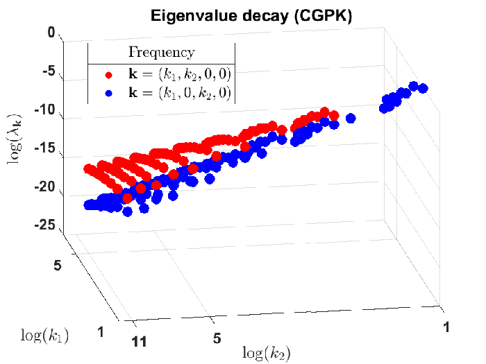
The graphs in Figure 4 show the eigenvalues of the CGPK kernel evaluated numerically for a three-layer network. The figure shows the eigenvalues for frequencies kk in 1-4 pixels. The slope of these lines, which depicts the exponent of the decay of the corresponding eigenvalues, is in good correspondence with our theory. Moreover, the decay rate is higher for frequencies spread over more pixels. This can be contrasted with the eigenvalues for the Gaussian Process Kernel for a fully connected network (FC-GPK) shown in Figure 5. For that kernel the decay rate is the same regardless of the pixel spread of frequencies, as is indicated by the parallel lines in the graph, and is empirically roughly equal to the maximal decay rate obtained for CGPK with 4 pixels. Figure 4 further shows the eigenvalues obtained with two frequency patterns, (k1,k2,0,0,…)(k_{1},k_{2},0,0,...) and (k1,0,k2,0,…)(k_{1},0,k_{2},0,...). As is predicted by our theory, while the decay rate for both patterns is similar, the latter eigenvalues are smaller than the former ones by a multiplicative constant.

Refer to caption
Refer to caption
Figure 4: Left: The eigenvalues of CGPK for frequency patterns that include either one non zero frequency (blue dots), two (orange), three (green) or four (maroon) identical frequencies. The slopes (respectively, −5.63-5.63, −7.71-7.71, −9.3-9.3 and −11.5-11.5) indicate the exponent for each pattern. (d=4d=4, ζ=3\zeta=3, q=2q=2, L=3L=3). Right: The eigenvalues of CGPK for two frequency patterns that include exactly two non zero frequency, either next to each other (red dots) or separated by one zero frequency (blue). Consistent with our theory, the eigenvalues obtained with non-zero frequencies next to each other are larger than those obtained with the same frequencies but separated (d=4d=4, ζ=3\zeta=3, q=2q=2, L=3L=3).
Refer to caption
Figure 5: The eigenvalues of FC-GPK on 𝕄​𝕊​(ζ,d)\mathbb{MS}(\zeta,d) for frequency patterns that include either one non zero frequency (blue dots), two (yellow), three (orange) or four (maroon) identical frequencies. The slopes (respectively, −12.4-12.4, −11.8-11.8, −11.6-11.6 and −11.7-11.7) indicate the exponent for each pattern. (d=4d=4, ζ=2\zeta=2, q=2q=2, L=3L=3 ).
Refer to caption
Refer to caption
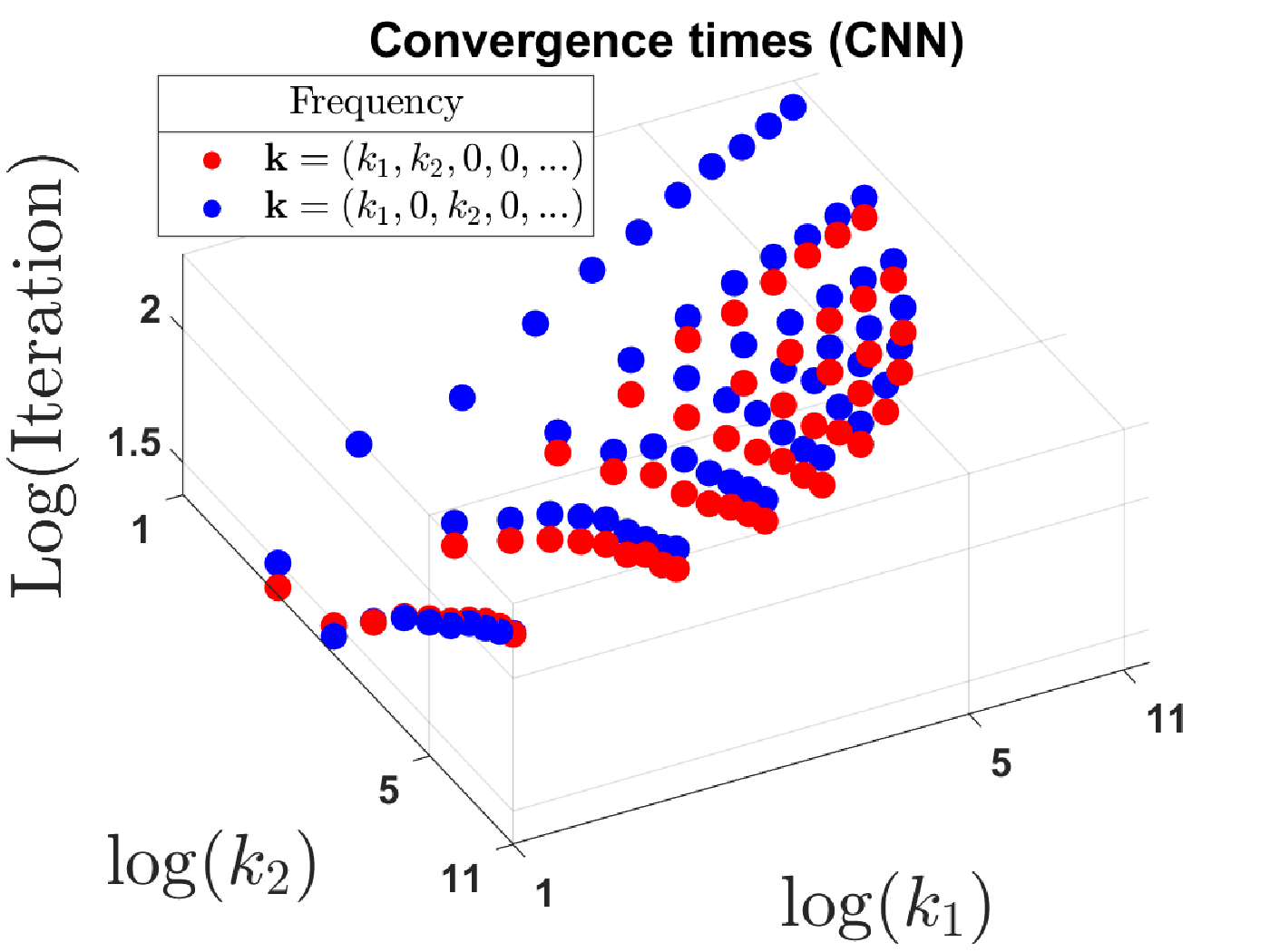
Figure 6: Training a CNN to fit eigenfunctions of the CNTK kernel (ζ=2\zeta=2, d=8d=8, q=3q=3, L=3L=3, m=1000m=1000). Each experiment is indicated by a circle or dot, depicting the number of GD iterations required to reach a 10−410^{-4} error as a function of (the product of) frequencies. Recall that, to the extent that GD for the CNN is similar to kernel GD of CNTK, the number of iterations needed to learn an eigenfunction should be inversely proportional to the corresponding eigenvalue. Left: The dashed line depicts a linear regression of these experiments. Its slope should reflect (up to a sign) the average decay of the eigenvalues. With a slope of 1.3, this regression line falls between the bounds (1.125 and 4) in Corollary 3.8. Right: Similar to Figure 4, we tested two frequency patterns. Convergence times for adjacent non-zero frequencies (red dots) are faster than their corresponding frequencies that are separated by one pixel (blue dots).
Refer to caption
Refer to caption
Figure 7: The eigenvalues of CGPK without the 1×11\times 1 convolution. Left: Eigenvalues for different frequency patterns that include either one non zero frequency (blue dots), two (red), three (orange) or four (maroon) identical frequencies. The slopes (respectively, −7.3-7.3, −7.5-7.5, −9.2-9.2 and −11.7-11.7) indicate the exponent for each pattern. (d=4d=4, ζ=2\zeta=2, q=2q=2, L=3L=3 ). Right: Eigenvalues for two frequency patterns that include exactly two non zero frequency, either next to each other (red dots) or separated by one zero frequency (blue). Black lines indicate differences from the values shown in Figure 4.

To examine the relevance of this analysis to CNNs of moderate size we trained CNNs to regress products of trigonometric functions, which are the eigenfunctions of the CNTK trace kernel with ζ=2\zeta=2. Figure 6 shows for each experiment the number of GD iterations needed to achieve a prescribed error. Recall that, to the extent that GD for the CNN is similar to kernel GD of CNTK, the number of iterations needed to learn an eigenfunction should be inversely proportional to the corresponding eigenvalue. The figure shows that overall the runtime lies between our predicted bounds. It also shows that it is faster to learn eigenfunctions involving two non zero frequencies adjacent to each other than ones that involve non-zero frequencies separated by one pixel, as is predicted by our theory.

Finally, our analysis uses network models which include a 1×11\times 1 convolution layer as the first layer. This simplifies our derivations and appears to have only limited effect on the results. In particular, it can be readily shown that for data distributed uniformly on the multisphere, the eigenfunctions of CGPK and CNTK without the 1×11\times 1 convolution are the SH-products (or their shift invariant sums in the case of GAP kernels). Figure 7 shows the eigenvalues of CGPK under the same conditions as in Figure 4 with the 1×11\times 1 convolution removed. Overall, similar decay patterns are observed, except that in the case of high frequency in one pixel (denoted ’(k,0,0,0)(k,0,0,0)’) the eigenvalues decay faster than with the 1×11\times 1 convolution.

4 Related Work

A number of papers analyze the spectral properties and generalization bounds for convolutional kernels, including CNTK. [9] derived explicit feature maps for CNTK. [30] developed spectral decomposition and generalization bounds for CNTK with one convolution layer and pooling with input in the nodes of the hyper-cube {−1,1}d\{-1,1\}^{d}. [16] considered CNTK with one convolutional layer and non-overlapping patches. Such input is equivalent to just 1×11\times 1 convolution layer in our setup. They developed a spectral theory for this case and used it to derive new generalization bounds. They showed that the eigenvalues decay is dictated by the patch size (corresponding to the number of channels in our setup). Their limited setup yields Mercer’s decomposition similar to that obtained with NTK for a two-layer fully connected network.

[29] considered a network with one convolution layer with patches of full image size and inputs drawn from the uniform distribution on either the sphere or the hypercube. Their work focuses on the benefits of group invariance in reducing the sample size. [10] considered general kernels that incorporate group invariance and derived a generalization bound based on counting the number of eigenfunctions of the kernel.

[28, 27] proposed a convolutional kernel network (CKN) that involves layers of patch extraction, convolution, and pooling. Pooling in this model is implemented by a convolution with a fixed filter such as a Gaussian, possibly followed by subsampling. We note that without subsampling, such pooling operation can effectively result in a fully connected layer. [34] proved that the set of functions produced by the CKN network that applies convolution with non-overlapping patches is contained in the RKHS of a kernel that includes just one convolution layer. Similar to our work, their work used inputs drawn from a multisphere, yielding eigenfunctions that are SH-products. They however bounded the eigenvalue decay for CKNs with polynomial activations at all except the first layer (with no convolutions in those layers). [7] extended this setup to enable convolution with overlapping patches and further derive generalization bounds. In contrast to these works, our work shows that the SH-products are the eigenfunctions of all multi-dot product kernels and further provides spectral analysis for CGPK and CNTK for multilayer CNNs.

[20] investigated the speed of convergence of gradient descent for equivariant networks with a fully connected layer followed by a fixed convolution layer in the context of image denoising. In a related work [39] used NTK for a two-layer network to relate denoising with CNNs to denoising with non-local filters.

Existing work also investigates CNNs from a non-kernel perspective, for example, by showing that multi-layer CNNs (and related networks) can efficiently learn compositional functions [33, 13].

5 Conclusion

Our paper has derived the eigenfunctions and corresponding eigenvalues of neural tangent kernels that describe overparameterized CNNs. This provides us with a clear and specific understanding of these networks, just as much prior work has done for fully connected networks. Of particular interest, our work provides a concrete understanding of the inductive bias produced by the hierarchical structure of deep CNNs. We see that CNNs can efficiently learn higher frequency functions than FC networks when these functions are spatially localized. We provide formulas that can show the trade-off points between higher frequency functions and spatial localization, and also show how architectural variations can affect these biases. We feel that this is a significant step towards understanding which features CNNs will learn, and how this may depend on network architecture.

Acknowledgement

This research is partially supported by the Israeli Council for Higher Education (CHE) via the Weizmann Data Science Research Center and by research grants from the Estate of Tully and Michele Plesser and the Anita James Rosen Foundation. David Jacobs is supported by the Guaranteeing AI Robustness Against Deception(GARD) program from DARPA and the National Science Foundation under grant no. IIS-1910132.

References

  • [1] Zeyuan Allen-Zhu, Yuanzhi Li, and Zhao Song. A convergence theory for deep learning via over-parameterization. In Kamalika Chaudhuri and Ruslan Salakhutdinov, editors, Proceedings of the 36th International Conference on Machine Learning, volume 97, pages 242–252, 2019.
  • [2] Sanjeev Arora, Simon S Du, Wei Hu, Zhiyuan Li, Ruslan Salakhutdinov, and Ruosong Wang. On exact computation with an infinitely wide neural net. arXiv preprint arXiv:1904.11955, 2019.
  • [3] Douglas Azevedo and Valdir A Menegatto. Eigenvalues of dot-product kernels on the sphere. Proceeding Series of the Brazilian Society of Computational and Applied Mathematics, 3(1), 2015.
  • [4] Francis Bach. Breaking the curse of dimensionality with convex neural networks. The Journal of Machine Learning Research, 18(1):629–681, 2017.
  • [5] Ronen Basri, Meirav Galun, Amnon Geifman, David Jacobs, Yoni Kasten, and Shira Kritchman. Frequency bias in neural networks for input of non-uniform density. In International Conference on Machine Learning, 2020.
  • [6] Ronen Basri, David Jacobs, Yoni Kasten, and Shira Kritchman. The convergence rate of neural networks for learned functions of different frequencies. In Advances in Neural Information Processing Systems, pages 4763–4772, 2019.
  • [7] Alberto Bietti. Approximation and learning with deep convolutional models: a kernel perspective. arXiv preprint arXiv:2102.10032, 2021.
  • [8] Alberto Bietti and Francis Bach. Deep equals shallow for relu networks in kernel regimes. arXiv preprint arXiv:2009.14397, 2020.
  • [9] Alberto Bietti and Julien Mairal. On the inductive bias of neural tangent kernels. arXiv preprint arXiv:1905.12173, 2019.
  • [10] Alberto Bietti, Luca Venturi, and Joan Bruna. On the sample complexity of learning with geometric stability. arXiv preprint arXiv:2106.07148, 2021.
  • [11] Lin Chen and Sheng Xu. Deep neural tangent kernel and laplace kernel have the same rkhs. arXiv preprint arXiv:2009.10683, 2020.
  • [12] Youngmin Cho and Lawrence Saul. Kernel methods for deep learning. In Y. Bengio, D. Schuurmans, J. Lafferty, C. Williams, and A. Culotta, editors, Advances in Neural Information Processing Systems, volume 22. Curran Associates, Inc., 2009.
  • [13] Nadav Cohen, Or Sharir, and Amnon Shashua. On the expressive power of deep learning: A tensor analysis. In Vitaly Feldman, Alexander Rakhlin, and Ohad Shamir, editors, 29th Annual Conference on Learning Theory, volume 49 of Proceedings of Machine Learning Research, pages 698–728, Columbia University, New York, New York, USA, 23–26 Jun 2016. PMLR.
  • [14] Abdallah Dhahri. Multi-variable orthogonal polynomials. arXiv preprint arXiv:1401.5434, 2014.
  • [15] Simon S. Du, Jason D. Lee, Haochuan Li, Liwei Wang, and Xiyu Zhai. Gradient descent finds global minima of deep neural networks. In Kamalika Chaudhuri and Ruslan Salakhutdinov, editors, Proceedings of the 36th International Conference on Machine Learning, ICML 2019, 9-15 June 2019, Long Beach, California, USA, volume 97, pages 1675–1685, 2019.
  • [16] Alessandro Favero, Francesco Cagnetta, and Matthieu Wyart. Locality defeats the curse of dimensionality in convolutional teacher-student scenarios. arXiv preprint arXiv:2106.08619, 2021.
  • [17] Philippe Flajolet and Robert Sedgewick. Analytic combinatorics. cambridge University press, 2009.
  • [18] Helmut Groemer. Geometric applications of Fourier series and spherical harmonics, volume 61. Cambridge University Press, 1996.
  • [19] Kaiming He, Xiangyu Zhang, Shaoqing Ren, and Jian Sun. Deep residual learning for image recognition. In Proceedings of the IEEE conference on computer vision and pattern recognition, pages 770–778, 2016.
  • [20] Reinhard Heckel and Mahdi Soltanolkotabi. Denoising and regularization via exploiting the structural bias of convolutional generators. arXiv preprint arXiv:1910.14634, 2019.
  • [21] Arthur Jacot, Franck Gabriel, and Clement Hongler. Neural tangent kernel: Convergence and generalization in neural networks. In S. Bengio, H. Wallach, H. Larochelle, K. Grauman, N. Cesa-Bianchi, and R. Garnett, editors, Advances in Neural Information Processing Systems 31, pages 8571–8580. 2018.
  • [22] Jiwon Kim, Jung Kwon Lee, and Kyoung Mu Lee. Accurate image super-resolution using very deep convolutional networks. In Proceedings of the IEEE conference on computer vision and pattern recognition, pages 1646–1654, 2016.
  • [23] Alex Krizhevsky, Ilya Sutskever, and Geoffrey E Hinton. Imagenet classification with deep convolutional neural networks. In F. Pereira, C. J. C. Burges, L. Bottou, and K. Q. Weinberger, editors, Advances in Neural Information Processing Systems, volume 25. Curran Associates, Inc., 2012.
  • [24] Y. Lecun, L. Bottou, Y. Bengio, and P. Haffner. Gradient-based learning applied to document recognition. Proceedings of the IEEE, 86(11):2278–2324, 1998.
  • [25] Christian Ledig, Lucas Theis, Ferenc Huszár, Jose Caballero, Andrew Cunningham, Alejandro Acosta, Andrew Aitken, Alykhan Tejani, Johannes Totz, Zehan Wang, et al. Photo-realistic single image super-resolution using a generative adversarial network. In Proceedings of the IEEE conference on computer vision and pattern recognition, pages 4681–4690, 2017.
  • [26] Wenjie Luo, Yujia Li, Raquel Urtasun, and Richard Zemel. Understanding the effective receptive field in deep convolutional neural networks. Advances in neural information processing systems, 29, 2016.
  • [27] Julien Mairal. End-to-end kernel learning with supervised convolutional kernel networks. Advances in neural information processing systems, 29:1399–1407, 2016.
  • [28] Julien Mairal, Piotr Koniusz, Zaid Harchaoui, and Cordelia Schmid. Convolutional kernel networks. In Z. Ghahramani, M. Welling, C. Cortes, N. Lawrence, and K. Q. Weinberger, editors, Advances in Neural Information Processing Systems, volume 27. Curran Associates, Inc., 2014.
  • [29] Song Mei, Theodor Misiakiewicz, and Andrea Montanari. Learning with invariances in random features and kernel models. arXiv preprint arXiv:2102.13219, 2021.
  • [30] Theodor Misiakiewicz and Song Mei. Learning with convolution and pooling operations in kernel methods. arXiv preprint arXiv:2111.08308, 2021.
  • [31] Claus Müller. Analysis of spherical symmetries in Euclidean spaces, volume 129. Springer Science & Business Media, 2012.
  • [32] Roman Novak, Lechao Xiao, Jaehoon Lee, Yasaman Bahri, Greg Yang, Jiri Hron, Daniel A Abolafia, Jeffrey Pennington, and Jascha Sohl-Dickstein. Bayesian deep convolutional networks with many channels are gaussian processes. arXiv preprint arXiv:1810.05148, 2018.
  • [33] Tomaso Poggio, Hrushikesh Mhaskar, Lorenzo Rosasco, Brando Miranda, and Qianli Liao. Why and when can deep-but not shallow-networks avoid the curse of dimensionality: a review. International Journal of Automation and Computing, 14(5):503–519, 2017.
  • [34] Meyer Scetbon and Zaid Harchaoui. Harmonic decompositions of convolutional networks. In International Conference on Machine Learning, pages 8522–8532. PMLR, 2020.
  • [35] Meyer Scetbon and Zaid Harchaoui. A spectral analysis of dot-product kernels. In International Conference on Artificial Intelligence and Statistics, pages 3394–3402. PMLR, 2021.
  • [36] Aidan Schumann. Multivariate bell polynomials and derivatives of composed functions. arXiv preprint arXiv:1903.03899, 2019.
  • [37] Karen Simonyan and Andrew Zisserman. Very deep convolutional networks for large-scale image recognition. In International Conference on Learning Representations, 2015.
  • [38] Alex J Smola, Zoltan L Ovari, Robert C Williamson, et al. Regularization with dot-product kernels. Advances in neural information processing systems, pages 308–314, 2001.
  • [39] Julian Tachella, Junqi Tang, and Mike Davies. The neural tangent link between cnn denoisers and non-local filters. In Proceedings of the IEEE/CVF Conference on Computer Vision and Pattern Recognition (CVPR), pages 8618–8627, June 2021.
  • [40] Dmitry Ulyanov, Andrea Vedaldi, and Victor Lempitsky. Deep image prior. In Proceedings of the IEEE conference on computer vision and pattern recognition, pages 9446–9454, 2018.

Appendix

Appendix A Multi-dot product kernels

In this section we prove results presented in Section 3.1.

Lemma A.1.

CGPK-EqNet and CNTK-EqNet are multi-dot product kernels.

Proof.

The proof follows directly from the derivation of the kernels in Section 2.2. Note that CGPK-EqNet is given by Σ~11(L)\tilde{\Sigma}_{11}^{(L)} and CNTK-EqNet by Θ~11(L)\tilde{\Theta}_{11}^{(L)}, and their recursive definition only involve elements of Σ~(l)\tilde{\Sigma}^{(l)} and Θ~(l)\tilde{\Theta}^{(l)} in which i=ji=j. Moreover, by definition the diagonal elements of Σ(0)\Sigma^{(0)} and Θ(0)\Theta^{(0)} are ⟨𝐱(i),𝐳(i)⟩\langle\mathbf{x}^{(i)},\mathbf{z}^{(i)}\rangle for i∈[d]i\in[d], implying the lemma. ∎

A.1 Multivariate Gegenbauer Polynomials

We next extend basic results derived for functions on the sphere to the multisphere 𝕄​𝕊​(ζ,d)\mathbb{MS}(\zeta,d). These results will assist us later to prove Mercer’s decomposition for multi-dot product kernels in the subsequent section.

We consider the set of Gegenbauer polynomials {Qk(ζ)​(t)}k≥0\{Q_{k}^{(\zeta)}(t)\}_{k\geq 0} that are orthogonal in L2​[−1,1]L_{2}[-1,1] w.r.t. the weight function (1−t2)(ζ−3)/2(1-t^{2})^{(\zeta-3)/2} and omit the superscript. Inspired by [14], we define multivariate Gegenbauer polynomials, using facts from harmonic analysis on the sphere. (See references [18, 31] for background on spherical harmonics and Gegenbauer polynomials). We denote by |𝕊ζ−1||\mathbb{S}^{\zeta-1}| the area of the sphere 𝕊ζ−1\mathbb{S}^{\zeta-1}.

Definition A.2.

For k≥0k\geq 0, let Qk​(t):[−1,1]→ℝQ_{k}(t):[-1,1]\rightarrow\mathbb{R} be the (univariate) Gegenbauer polynomial of degree kk. Then, the multivariate Gegenbauer polynomial of order 𝐤\mathbf{k} is Q𝐤​(𝐭):[−1,1]d→ℝQ_{\mathbf{k}}(\mathbf{t}):[-1,1]^{d}\rightarrow\mathbb{R}, defined by

Q𝐤​(𝐭)=Qk1​(t1)⋅Qk2​(t2)⋅…⋅Qkd​(td).\displaystyle Q_{\mathbf{k}}(\mathbf{t})=Q_{k_{1}}(t_{1})\cdot Q_{k_{2}}(t_{2})\cdot...\cdot Q_{k_{{d}}}(t_{{d}}).

These multivariate Gegenbauer polynomials enjoy several properties that they inherit from their univariate counterpart.

Lemma A.3.

Let Pk​(𝐭)P_{k}(\mathbf{t}) denote the space of polynomials of degree ≤k\leq k with variables 𝐭∈[−1,1]d\mathbf{t}\in[-1,1]^{d}. Then, the set {Q𝐢​(𝐭)}𝐢=0|𝐢|=k\{Q_{\mathbf{i}}(\mathbf{t})\}_{\mathbf{i}=0}^{|\mathbf{i}|=k} is an orthogonal basis of Pk​(𝐭)P_{k}(\mathbf{t}) w.r.t. the weight function (1−t2)(ζ−3)/2(1-t^{2})^{(\zeta-3)/2} (with 𝐢=(i1,…,id)\mathbf{i}=(i_{1},\ldots,i_{{d}}) and |𝐢|=i1+…+id|\mathbf{i}|=i_{1}+\ldots+i_{{d}}).

Proof.

Let p⁡(𝐭)=∑𝐢=0|𝐢|=ka𝐢​𝐭𝐢∈Pk​(𝐭)p(\mathbf{t})=\sum_{\mathbf{i}=0}^{|\mathbf{i}|=k}a_{\mathbf{i}}\mathbf{t}^{\mathbf{i}}\in P_{k}(\mathbf{t}). Since the univariate Gegenbauer polynomials form an orthogonal basis, for every 0≤ni≤k0\leq n_{i}\leq k and i∈[d]i\in[{d}] we can write tini=∑j=0niaj(ni)​Qj​(ti)t_{i}^{n_{i}}=\sum_{j=0}^{n_{i}}a^{(n_{i})}_{j}Q_{j}(t_{i}), where aj(ni)∈ℝa_{j}^{(n_{i})}\in\mathbb{R}, and the superscript is used to emphasize that the expansion depends on nin_{i}. Therefore, p⁡(𝐭)p(\mathbf{t}) can be written as

p⁡(𝐭)\displaystyle p(\mathbf{t}) =∑𝐧=0|𝐧|=ka𝐧𝐭𝐧=∑𝐧=0|𝐧|=ka𝐧(∑j=0n1aj(n1)Qj(t1))⋅..⋅(∑j=0ndaj(nd)Qj(td))\displaystyle=\sum_{\mathbf{n}=0}^{|\mathbf{n}|=k}a_{\mathbf{n}}\mathbf{t}^{\mathbf{n}}=\sum_{\mathbf{n}=0}^{|\mathbf{n}|=k}a_{\mathbf{n}}\left(\sum_{j=0}^{n_{1}}a^{(n_{1})}_{j}Q_{j}(t_{1})\right)\cdot..\cdot\left(\sum_{j=0}^{n_{d}}a^{(n_{d})}_{j}Q_{j}(t_{{d}})\right)
=∑𝐧=0|𝐧|=k(1)⁡a~𝐧​Qn1​(t1)​Qi2​(t2)⋅…⋅Qnd​(td)=∑𝐧=0|𝐧|=ka~𝐧​Q𝐧​(𝐭),\displaystyle=^{(1)}\sum_{\mathbf{n}=0}^{|\mathbf{n}|=k}\tilde{a}_{\mathbf{n}}Q_{n_{1}}(t_{1})Q_{i_{2}}(t_{2})\cdot\ldots\cdot Q_{n_{d}}(t_{d})=\sum_{\mathbf{n}=0}^{|\mathbf{n}|=k}\tilde{a}_{\mathbf{n}}Q_{\mathbf{n}}(\mathbf{t}),

where (1) is obtained by applying the distributive law with the fact that n1,..,nd≤kn_{1},..,n_{{d}}\leq k. finally, a~𝐢\tilde{a}_{\mathbf{i}} can be computed explicitly from a𝐢a_{\mathbf{i}} and {aj(ni)}\{a_{j}^{(n_{i})}\}.

We have shown that Pk​(𝐭)P_{k}(\mathbf{t}) is spanned by the set {Q𝐢​(𝐭)}𝐢=0|𝐢|=k\{Q_{\mathbf{i}}(\mathbf{t})\}_{\mathbf{i}=0}^{|\mathbf{i}|=k}. Next, we show that this set is orthogonal with respect to the measure ∏r=1d((1−tr2)ζ−32)\prod_{r=1}^{d}\left((1-t_{r}^{2})^{\frac{\zeta-3}{2}}\right). Let 𝐢\mathbf{i} and 𝐣\mathbf{j} be two vectors of indices. Then, we have that

∫[−1,1]d\displaystyle\int_{[-1,1]^{d}} Q𝐢​(𝐭)​Q𝐣​(𝐭)​∏r=1d(1−tr2)ζ−32​d​t1⋅…⋅d​td=∏r=1d(∫[−1,1]Qir​(tr)​Qjr​(tr)​(1−tr2)ζ−32​d​tr)\displaystyle Q_{\mathbf{i}}(\mathbf{t})Q_{\mathbf{j}}(\mathbf{t})\prod_{r=1}^{d}(1-t_{r}^{2})^{\frac{\zeta-3}{2}}dt_{1}\cdot\ldots\cdot dt_{{d}}=\prod_{r=1}^{d}\left(\int_{[-1,1]}Q_{i_{r}}(t_{r})Q_{j_{r}}(t_{r})(1-t_{r}^{2})^{\frac{\zeta-3}{2}}dt_{r}\right)
=\displaystyle= (|𝕊ζ−1||𝕊ζ−2|)d​(∏r=1dN⁡(ζ,ir))−1​δi1,j1⋅δi2,j2⋅…⋅δid,jd,\displaystyle\left(\frac{|\mathbb{S}^{\zeta-1}|}{|\mathbb{S}^{\zeta-2}|}\right)^{d}\left(\prod_{r=1}^{d}N(\zeta,i_{r})\right)^{-1}\delta_{i_{1},j_{1}}\cdot\delta_{i_{2},j_{2}}\cdot\ldots\cdot\delta_{i_{{d}},j_{{d}}},

where the last equality is due to the orthogonality property of the univariate Gegenbauer polynomials. This concludes the proof. ∎

The relation of the multivariate Gegenbauer polynomials to the SH-products is formulated in the following lemma.

Lemma A.4.

Let 𝐱,𝐳∈𝕄​𝕊​(ζ,d)\mathbf{x},\mathbf{z}\in\mathbb{MS}(\zeta,d). It holds that

Q𝐤(⟨𝐱(1),𝐳(1)⟩,..,⟨𝐱(i),𝐳(j)⟩,..,⟨𝐱(d),𝐳(d)⟩)=|𝕊ζ−1|d(∏r=1dN(q,kr))−1∑𝐣:jr∈[N⁡(ζ,kr)]Y𝐤,𝐣(𝐱)Y𝐤,𝐣(𝐳),\displaystyle Q_{\mathbf{k}}(\langle\mathbf{x}^{(1)},\mathbf{z}^{(1)}\rangle,..,\langle\mathbf{x}^{(i)},\mathbf{z}^{(j)}\rangle,..,\langle\mathbf{x}^{({{d}})},\mathbf{z}^{({{d}})}\rangle)=|\mathbb{S}^{\zeta-1}|^{d}\left(\prod_{r=1}^{d}N(q,k_{r})\right)^{-1}\sum_{\mathbf{j}:j_{r}\in[N(\zeta,k_{r})]}Y_{\mathbf{k},\mathbf{j}}(\mathbf{x})Y_{\mathbf{k},\mathbf{j}}(\mathbf{z}),

where Y𝐤,𝐣​(𝐱)Y_{\mathbf{k},\mathbf{j}}(\mathbf{x}) is homogeneous polynomial of degree k1+..+kdk_{1}+..+k_{{d}}. Y𝐤,𝐣​(𝐱)Y_{\mathbf{k},\mathbf{j}}(\mathbf{x}) is further given by SH-products, i.e., Y𝐤,𝐣​(𝐱)=∏i=1dYki,ji​(𝐱(i))Y_{\mathbf{k},\mathbf{j}}(\mathbf{x})=\prod_{i=1}^{{{d}}}Y_{k_{i},j_{i}}(\mathbf{x}^{(i)}), where Yki​jiY_{k_{i}j_{i}} are spherical harmonics in 𝕊ζ−1\mathbb{S}^{\zeta-1}, and N⁡(ζ,ki)N(\zeta,k_{i}) are the number of harmonics of frequency kik_{i} in 𝕊ζ−1\mathbb{S}^{\zeta-1}.

Proof.

By the definition of the multivariate Gegenbauer polynomials and the univariate addition theorem [38] we get

Q𝐤\displaystyle Q_{\mathbf{k}} (⟨𝐱(1),𝐳(1)⟩,…,⟨𝐱(i),𝐳(j)⟩,…,⟨𝐱(d),𝐳(d)⟩)=Qk1​(⟨𝐱(1),𝐳(1)⟩)⋅…⋅Qkd​(⟨𝐱(d),𝐳(d)⟩)\displaystyle(\langle\mathbf{x}^{(1)},\mathbf{z}^{(1)}\rangle,...,\langle\mathbf{x}^{(i)},\mathbf{z}^{(j)}\rangle,...,\langle\mathbf{x}^{({{d}})},\mathbf{z}^{({{d}})}\rangle)=Q_{k_{1}}(\langle\mathbf{x}^{(1)},\mathbf{z}^{(1)}\rangle)\cdot...\cdot Q_{k_{{d}}}(\langle\mathbf{x}^{({{d}})},\mathbf{z}^{({{d}})}\rangle)
=\displaystyle= (|𝕊ζ−1|N⁡(ζ,k1)​∑j1=1N⁡(ζ,k1)Yk1,j1​(𝐱(1))​Yk1,j1​(𝐳(1)))⋅…⋅(|𝕊ζ−1|N⁡(ζ,kd)​∑jd=1N⁡(ζ,kd)Ykd,jd​(𝐱(d))​Ykd,jd​(𝐳(d)))\displaystyle\left(\frac{|\mathbb{S}^{\zeta-1}|}{N(\zeta,k_{1})}\sum_{j_{1}=1}^{N(\zeta,k_{1})}Y_{k_{1},j_{1}}(\mathbf{x}^{(1)})Y_{k_{1},j_{1}}(\mathbf{z}^{(1)})\right)\cdot\ldots\cdot\left(\frac{|\mathbb{S}^{\zeta-1}|}{N(\zeta,k_{{d}})}\sum_{j_{{d}}=1}^{N(\zeta,k_{{d}})}Y_{k_{{d}},j_{{d}}}(\mathbf{x}^{({{d}})})Y_{k_{{d}},j_{{d}}}(\mathbf{z}^{({{d}})})\right)
=\displaystyle= (∏i=1d|𝕊ζ−1|N⁡(ζ,ki))​∑𝐣=(1,…,1)𝐣=(N⁡(ζ,k1),…,N⁡(ζ,kd))∏i=1dYki,ji​(𝐱(i))​Yki,ji​(𝐳(i))\displaystyle\left(\prod_{i=1}^{{{d}}}\frac{|\mathbb{S}^{\zeta-1}|}{N(\zeta,k_{i})}\right)\sum_{\mathbf{j}=(1,...,1)}^{\mathbf{j}=(N(\zeta,k_{1}),...,N(\zeta,k_{{d}}))}\prod_{i=1}^{{{d}}}Y_{k_{i},j_{i}}(\mathbf{x}^{(i)})Y_{k_{i},j_{i}}(\mathbf{z}^{(i)})
:⁣=\displaystyle:= (∏i=1d|𝕊ζ−1|N⁡(ζ,ki))∑𝐣:ji∈[N⁡(ζ,ki)]Y𝐤,𝐣(𝐱)Y𝐤,𝐣(𝐳).\displaystyle\left(\prod_{i=1}^{{{d}}}\frac{|\mathbb{S}^{\zeta-1}|}{N(\zeta,k_{i})}\right)\sum_{\mathbf{j}:j_{i}\in[N(\zeta,k_{i})]}Y_{\mathbf{k},\mathbf{j}}(\mathbf{x})Y_{\mathbf{k},\mathbf{j}}(\mathbf{z}).

Note that the homogeneity of the SH-products Y𝐤,𝐣​(𝐱)Y_{\mathbf{k},\mathbf{j}}(\mathbf{x}) is a direct result of the homogeneity of the spherical harmonics Yki,jiY_{k_{i},j_{i}}. ∎

Lemma A.5.

The set {Y𝐤,𝐣}\{Y_{\mathbf{k},\mathbf{j}}\} are orthonormal w.r.t uniform measure in 𝕄​𝕊​(ζ,d)\mathbb{MS}(\zeta,d).

Proof.

We have that

∫𝕄​𝕊​(ζ,d)Y𝐤,𝐣​(𝐱)​Y𝐤′,𝐣′​(𝐱)​𝑑𝐱=\displaystyle\int_{\mathbb{MS}(\zeta,d)}Y_{\mathbf{k},\mathbf{j}}(\mathbf{x})Y_{\mathbf{k}^{\prime},\mathbf{j}^{\prime}}(\mathbf{x})d\mathbf{x}= ∫𝕄​𝕊​(ζ,d)(∏i=1dYki,ji​(𝐱(i)))​(∏i=1dYki′,ji′​(𝐱(i)))​𝑑𝐱\displaystyle\int_{\mathbb{MS}(\zeta,d)}\left(\prod_{i=1}^{{{d}}}Y_{k_{i},j_{i}}(\mathbf{x}^{(i)})\right)\left(\prod_{i=1}^{{{d}}}Y_{k^{\prime}_{i},j^{\prime}_{i}}(\mathbf{x}^{(i)})\right)d\mathbf{x}
=\displaystyle= ∏i=1d(∫𝕊ζ−1Yki,ji​(𝐱(i))​Yki′,ji′​(𝐱(i))​d​𝐱(i))=∏i=1dδki,ki′⋅δji,ji′.\displaystyle\prod_{i=1}^{{{d}}}\left(\int_{\mathbb{S}^{\zeta-1}}Y_{k_{i},j_{i}}(\mathbf{x}^{(i)})Y_{k^{\prime}_{i},j^{\prime}_{i}}(\mathbf{x}^{(i)})d\mathbf{x}^{(i)}\right)=\prod_{i=1}^{d}\delta_{k_{i},k^{\prime}_{i}}\cdot\delta_{j_{i},j^{\prime}_{i}}.

∎

A.2 Mercer’s decomposition

In this section we prove that the eigenfunctions of multi dot-product kernels consist of products of spherical harmonics. We further provide a way to calculate the eigenvalues using products of Gegenbauer polynomials.

Lemma A.6.

Let −𝐤\mathrlap{{}^{-}}\boldsymbol{k} be a multi-dot product kernel. Then, the eigenfunctions of 𝐤−(𝐱,⋅)\mathrlap{{}^{-}}\boldsymbol{k}(\mathbf{x},\cdot) w.r.t uniform measure on 𝕄​𝕊​(ζ,d)\mathbb{MS}(\zeta,d) are the SH-products. Namely, the eigenfunctions are

{Y𝐤,𝐣(𝐱)=∏i=1dYki​ji(𝐱(i))}𝐤≥0,ji∈[N⁡(q,ki)],\displaystyle\left\{Y_{\mathbf{k},\mathbf{j}}(\mathbf{x})=\prod_{i=1}^{{{d}}}Y_{k_{i}j_{i}}\left(\mathbf{x}^{(i)}\right)\right\}_{\mathbf{k}\geq 0,~j_{i}\in[N(q,k_{i})]},

where Yki​jiY_{k_{i}j_{i}} are the Spherical Harmonics in 𝕊ζ−1\mathbb{S}^{\zeta-1}, and N⁡(ζ,ki)N(\zeta,k_{i}) are the number of harmonics of frequency kik_{i} in 𝕊ζ−1\mathbb{S}^{\zeta-1}. The eigenvalues, λ𝐤\lambda_{\mathbf{k}}, can be calculated using products of (univariate) Gegenbauer polynomials as follows,

λ𝐤=C(ζ,d)∫[−1,1]d𝒌−(𝐭)∏i=1dQki(ti)(1−ti2)ζ−32d𝐭\displaystyle\lambda_{\mathbf{k}}=C(\zeta,d)\int_{[-1,1]^{d}}\mathrlap{{}^{-}}\boldsymbol{k}(\mathbf{t})\prod_{i=1}^{d}Q_{k_{i}}(t_{i})(1-t_{i}^{2})^{\frac{\zeta-3}{2}}d\mathbf{t}

where {Qk​(t)}\{Q_{k}(t)\} is the set of orthogonal Gegenbauer polynomials w.r.t the weights (1−ti2)ζ−32(1-t_{i}^{2})^{\frac{\zeta-3}{2}}, and C⁡(ζ,d)C(\zeta,d) is a constant that depends on both ζ\zeta and dd.

Proof.

Let −𝒌\mathrlap{{}^{-}}\boldsymbol{k} be a multi-dot product kernel. By definition for such kernel, there exists a multivariate analytic function κ\kappa such that 𝒌(L)−(𝐱,𝐳)=κ(⟨𝐱(1),𝐳(1)⟩,…,⟨𝐱(d),𝐳(d)⟩)\mathrlap{{}^{-}}\boldsymbol{k}^{(L)}(\mathbf{x},\mathbf{z})=\kappa(\langle\mathbf{x}^{(1)},\mathbf{z}^{(1)}\rangle,...,\langle\mathbf{x}^{(d)},\mathbf{z}^{(d)}\rangle). Using lemma A.3, {Q𝐤}\{Q_{\mathbf{k}}\} form an orthogonal basis in [−1,1]d[-1,1]^{d}. Therefore, it can be readily shown (similar to [38]) that, κ\kappa can be written as

κ(t1,..,td):=κ(𝐭)=∑𝐤≥0(∏i=1dN(ζ,ki)|𝕊ζ−2||𝕊ζ−1|)Q𝐤(𝐭)∫[−1,1]dκ(𝐭~)Q𝐤(𝐭~)∏i=1d(1−t~i2)ζ−32d𝐭~:=∑𝐤≥0λ𝐤Q𝐤(𝐭).\displaystyle\kappa(t_{1},..,t_{{d}}):=\kappa(\mathbf{t})=\sum_{\mathbf{k}\geq 0}\left(\prod_{i=1}^{d}N(\zeta,k_{i})\frac{|\mathbb{S}^{\zeta-2}|}{|\mathbb{S}^{\zeta-1}|}\right)Q_{\mathbf{k}}(\mathbf{t})\int_{[-1,1]^{d}}\kappa(\tilde{\mathbf{t}})Q_{\mathbf{k}}(\tilde{\mathbf{t}})\prod_{i=1}^{d}(1-\tilde{t}_{i}^{2})^{\frac{\zeta-3}{2}}d\tilde{\mathbf{t}}:=\sum_{\mathbf{k}\geq 0}\lambda_{\mathbf{k}}Q_{\mathbf{k}}(\mathbf{t}).

Lemma A.4 implies

Q𝐤(⟨𝐱(1),𝐳(1)⟩,..,⟨𝐱(i),𝐳(j)⟩,..,⟨𝐱(d),𝐳(d)⟩)=|𝕊ζ−1|d∏i=1dN⁡(ζ,ki)∑𝐣:ji∈[N⁡(ζ,ki)]Y𝐤,𝐣(𝐱)Y𝐤,𝐣(𝐳),\displaystyle Q_{\mathbf{k}}(\langle\mathbf{x}^{(1)},\mathbf{z}^{(1)}\rangle,..,\langle\mathbf{x}^{(i)},\mathbf{z}^{(j)}\rangle,..,\langle\mathbf{x}^{({{d}})},\mathbf{z}^{({{d}})}\rangle)=\frac{|\mathbb{S}^{\zeta-1}|^{d}}{\prod_{i=1}^{{{d}}}N(\zeta,k_{i})}\sum_{\mathbf{j}:j_{i}\in[N(\zeta,k_{i})]}Y_{\mathbf{k},\mathbf{j}}(\mathbf{x})Y_{\mathbf{k},\mathbf{j}}(\mathbf{z}),

yielding

𝒌−(𝐱,𝐳)=∑𝐤≥0λ𝐤∑𝐣:ji∈[N⁡(ζ,ki)]Y𝐤,𝐣(𝐱)Y𝐤,𝐣(𝐳).\displaystyle\mathrlap{{}^{-}}\boldsymbol{k}(\mathbf{x},\mathbf{z})=\sum_{\mathbf{k}\geq 0}\lambda_{\mathbf{k}}\sum_{\mathbf{j}:j_{i}\in[N(\zeta,k_{i})]}Y_{\mathbf{k},\mathbf{j}}(\mathbf{x})Y_{\mathbf{k},\mathbf{j}}(\mathbf{z}).

Since {Y𝐤,𝐣​(𝐱)}\{Y_{\mathbf{k},\mathbf{j}}(\mathbf{x})\} are orthonormal w.r.t. the uniform measure in 𝕄​𝕊​(ζ,d)\mathbb{MS}(\zeta,d) (Lemma A.5) we obtain that {Y𝐤,𝐣​(𝐱)}\{Y_{\mathbf{k},\mathbf{j}}(\mathbf{x})\} are the eigenfunctions of −𝒌(L)\mathrlap{{}^{-}}\boldsymbol{k}^{(L)}, with the corresponding eigenvalues {λ𝐤=|𝕊ζ−2|d∫[−1,1]d𝒌−(𝐭)∏i=1dQki(ti)(1−ti2)ζ−32d𝐭}\{\lambda_{\mathbf{k}}=|\mathbb{S}^{\zeta-2}|^{d}\int_{[-1,1]^{d}}\mathrlap{{}^{-}}\boldsymbol{k}(\mathbf{t})\prod_{i=1}^{d}Q_{k_{i}}(t_{i})(1-t_{i}^{2})^{\frac{\zeta-3}{2}}d\mathbf{t}\}. ∎

A.3 Proof of Lemma 3.1

Lemma A.7.

Let −𝐤\mathrlap{{}^{-}}\boldsymbol{k} be a multi-dot product kernel with the power series given in (2), where 𝐱(i),𝐳(i)∈𝕊ζ−1\mathbf{x}^{(i)},\mathbf{z}^{(i)}\in\mathbb{S}^{\zeta-1} respectively are pixels in 𝐱,𝐳\mathbf{x},\mathbf{z}. Then, the eigenvalues λ𝐤(𝐤−)\lambda_{\mathbf{k}}(\mathrlap{{}^{-}}\boldsymbol{k}) of −𝐤\mathrlap{{}^{-}}\boldsymbol{k} are given by λ𝐤(𝐤−)=|𝕊ζ−2|d∑𝐬≥0b𝐤+2​𝐬∏i=1dλki(tki+2​si)\lambda_{\mathbf{k}}(\mathrlap{{}^{-}}\boldsymbol{k})=\left|\mathbb{S}^{\zeta-2}\right|^{d}\sum_{\mathbf{s}\geq 0}b_{\mathbf{k}+2\mathbf{s}}\prod_{i=1}^{{d}}\lambda_{k_{i}}(t^{k_{i}+2s_{i}}), where |𝕊ζ−2||\mathbb{S}^{\zeta-2}| is the surface area of 𝕊ζ−2\mathbb{S}^{\zeta-2}, and λk​(tn)\lambda_{k}(t^{n}) is the kk’th eigenvalue of tnt^{n}, given by

λk​(tn)=n!(n−k)!​2k+1​Γ⁡(ζ−12)​Γ​(n−k+12)Γ⁡(n−k+ζ2)\displaystyle\lambda_{k}(t^{n})=\frac{n!}{(n-k)!2^{k+1}}\frac{\Gamma\left(\frac{\zeta-1}{2}\right)\Gamma\left(\frac{n-k+1}{2}\right)}{\Gamma\left(\frac{n-k+\zeta}{2}\right)}

if n−kn-k is even and non-negative, while λk​(tn)=0\lambda_{k}(t^{n})=0 otherwise, and Γ\Gamma is the Gamma function.

Proof.

The proof follows the linearity of the integral operator. Let

𝒌−(𝐱,𝐳)=∑𝐧≥0b𝐧⟨𝐱(1),𝐳(1)⟩n1⋅…⋅⟨𝐱(d),𝐳(d)⟩nd,\displaystyle\mathrlap{{}^{-}}\boldsymbol{k}(\mathbf{x},\mathbf{z})=\sum_{\mathbf{n}\geq 0}b_{\mathbf{n}}\langle\mathbf{x}^{(1)},\mathbf{z}^{(1)}\rangle^{n_{1}}\cdot...\cdot\langle\mathbf{x}^{(d)},\mathbf{z}^{(d)}\rangle^{n_{d}}, (4)

and denote by C⁡(ζ,d)=|𝕊ζ−2|dC(\zeta,d)=\left|\mathbb{S}^{\zeta-2}\right|^{d}. Following Lemma A.6 the eigenvalues of −𝒌\mathrlap{{}^{-}}\boldsymbol{k} are given by

λ𝐤=\displaystyle\lambda_{\mathbf{k}}= C(ζ,d)∫[−1,1]d𝒌−(𝐭)∏i=1dQki(ti)(1−ti2)ζ−32dt1…dtd\displaystyle C(\zeta,d)\int_{[-1,1]^{d}}\mathrlap{{}^{-}}\boldsymbol{k}(\mathbf{t})\prod_{i=1}^{d}Q_{k_{i}}(t_{i})(1-t_{i}^{2})^{\frac{\zeta-3}{2}}dt_{1}...dt_{d}
=\displaystyle= C⁡(ζ,d)​∫[−1,1]d∑𝐧≥0b𝐧​𝐭𝐧​∏i=1dQki​(ti)​(1−ti2)ζ−32​d​t1​…​d​td\displaystyle C(\zeta,d)\int_{[-1,1]^{d}}\sum_{\mathbf{n}\geq 0}b_{\mathbf{n}}\mathbf{t}^{\mathbf{n}}\prod_{i=1}^{d}Q_{k_{i}}(t_{i})(1-t_{i}^{2})^{\frac{\zeta-3}{2}}dt_{1}...dt_{d}
=\displaystyle= C⁡(ζ,d)​∑𝐧≥0b𝐧​∏i=1d(∫[−1,1]tin​Qki​(ti)​(1−ti2)ζ−32​d​ti)=C⁡(ζ,d)​∑𝐧≥0b𝐧​∏i=1dλki​(tni).\displaystyle C(\zeta,d)\sum_{\mathbf{n}\geq 0}b_{\mathbf{n}}\prod_{i=1}^{d}\left(\int_{[-1,1]}t^{n}_{i}Q_{k_{i}}(t_{i})(1-t_{i}^{2})^{\frac{\zeta-3}{2}}dt_{i}\right)=C(\zeta,d)\sum_{\mathbf{n}\geq 0}b_{\mathbf{n}}\prod_{i=1}^{d}\lambda_{k_{i}}(t^{n_{i}}).

Also note from [3] that λk​(tn)=0\lambda_{k}(t^{n})=0 whenever n−kn-k is either odd or negative, implying the statement of the lemma. ∎

A consequence of the lemma above is that the eigenvalues of a kernel −𝒌\mathrlap{{}^{-}}\boldsymbol{k} can be bounded by the eigenvalues of other kernels if the power series coefficients of −𝒌\mathrlap{{}^{-}}\boldsymbol{k} are bounded by the respective coefficients of the other kernels. We summarize this in the following corollary:

Corollary A.8.

Let 𝐤−,𝐤u​p​p​e​r−,𝐤l​o​w​e​r−:𝕄𝕊(ζ,d)→ℝ\mathrlap{{}^{-}}\boldsymbol{k},\mathrlap{{}^{-}}\boldsymbol{k}^{upper},\mathrlap{{}^{-}}\boldsymbol{k}^{lower}:\mathbb{MS}(\zeta,d)\rightarrow\mathbb{R} be multi-dot product kernels. Assuming that for 𝐭∈[−1,1]d\mathbf{t}\in[-1,1]^{d},

𝒌−(𝐭)=∑𝐧b𝐧𝐭𝐧\displaystyle\mathrlap{{}^{-}}\boldsymbol{k}(\mathbf{t})=\sum_{\mathbf{n}}b_{\mathbf{n}}\mathbf{t}^{\mathbf{n}}
𝒌u​p​p​e​r−(𝐭)=∑𝐧b𝐧u​p​p​e​r𝐭𝐧\displaystyle\mathrlap{{}^{-}}\boldsymbol{k}^{upper}(\mathbf{t})=\sum_{\mathbf{n}}b^{upper}_{\mathbf{n}}\mathbf{t}^{\mathbf{n}}
𝒌l​o​w​e​r−(𝐭)=∑𝐧b𝐧l​o​w​e​r𝐭𝐧\displaystyle\mathrlap{{}^{-}}\boldsymbol{k}^{lower}(\mathbf{t})=\sum_{\mathbf{n}}b^{lower}_{\mathbf{n}}\mathbf{t}^{\mathbf{n}}

and suppose there exists 𝐤0\mathbf{k}_{0} such that for all 𝐧≥𝐤0\mathbf{n}\geq\mathbf{k}_{0}, 0≤c1​b𝐧l​o​w​e​r≤b𝐧≤c2​b𝐧u​p​p​e​r0\leq c_{1}b^{lower}_{\mathbf{n}}\leq b_{\mathbf{n}}\leq c_{2}b^{upper}_{\mathbf{n}}, with c1,c2>0c_{1},c_{2}>0. Then, for all 𝐤≥𝐤0\mathbf{k}\geq\mathbf{k}_{0},

c1λ𝐤(𝒌l​o​w​e​r−)≤λ𝐤(𝒌−)≤c2λ𝐤(𝒌u​p​p​e​r−)\displaystyle c_{1}\lambda_{\mathbf{k}}(\mathrlap{{}^{-}}\boldsymbol{k}^{lower})\leq\lambda_{\mathbf{k}}(\mathrlap{{}^{-}}\boldsymbol{k})\leq c_{2}\lambda_{\mathbf{k}}(\mathrlap{{}^{-}}\boldsymbol{k}^{upper}) (5)

This corollary is an immediate result from Lemma 3.1.

Appendix B Factorizable kernels

In this section we prove results presented in Section 3.2. We prove Theorem 3.2, which determines the eigenvalues of factorizable kernels whose power series coefficients decay at a polynomial rate. The following supporting lemma proves the theorem for d=1d=1.

Lemma B.1.

Let κ~​(t)=∑n=0∞a~n​tn\tilde{\kappa}(t)=\sum_{n=0}^{\infty}\tilde{a}_{n}t^{n} where a~n=O⁡(n−ν)\tilde{a}_{n}=O(n^{-\nu}) with ν>1\nu>1 and not integer. Then, the eigenvalues of κ~\tilde{\kappa} w.r.t. the uniform measure in 𝕊ζ−1\mathbb{S}^{\zeta-1} are

λk=Θ⁡(k−(ζ+2​ν−3)).\displaystyle\lambda_{k}=\Theta\left(k^{-(\zeta+2\nu-3)}\right).
Proof.

By applying Corollary A.8 with d=1{d}=1 we have that if f⁡(t)=∑n=0∞an​tnf(t)=\sum_{n=0}^{\infty}a_{n}t^{n} and g⁡(t)=∑n=0∞bn​tng(t)=\sum_{n=0}^{\infty}b_{n}t^{n} with c1​an≤bn≤c2​anc_{1}a_{n}\leq b_{n}\leq c_{2}a_{n} then it holds that λk​(g)=Θ⁡(λk​(f))\lambda_{k}(g)=\Theta(\lambda_{k}(f)). It is therefore enough to find f⁡(t)=∑n=0∞a~n​tnf(t)=\sum_{n=0}^{\infty}\tilde{a}_{n}t^{n} where a~n=O⁡(n−ν)\tilde{a}_{n}=O(n^{-\nu}) and then calculate its eigenvalues. By [17] (Thm. VI.1, page 381), the function f⁡(t)=(1−t)ν−1f(t)=(1-t)^{\nu-1}, where ν>1\nu>1 is non-integer, satisfies f⁡(t)=∑n=0∞a~n​tnf(t)=\sum_{n=0}^{\infty}\tilde{a}_{n}t^{n} with a~n=O⁡(n−ν)\tilde{a}_{n}=O\left(n^{-\nu}\right). Moreover, according to [8] (Thm. 7, page 17), the eigenvalues of f⁡(t)=(1−t)ν−1f(t)=(1-t)^{\nu-1} in 𝕊ζ−1\mathbb{S}^{\zeta-1} are

λk​(f)=c1​k−(ζ+2​ν−3),\displaystyle\lambda_{k}(f)=c_{1}k^{-(\zeta+2\nu-3)},

which concludes the proof. ∎

Relying on the lemma, we can now prove Theorem 3.2.

Theorem B.2.

Let −𝐤\mathrlap{{}^{-}}\boldsymbol{k} be a factorizable multi-dot product kernel, and let ℛ⊆[d]\mathcal{R}\subseteq[d] denote its receptive field. Suppose that −𝐤\mathrlap{{}^{-}}\boldsymbol{k} can be written as a multivariate power series, 𝐤−(𝐭)=∑𝐧≥0b𝐧𝐭𝐧\mathrlap{{}^{-}}\boldsymbol{k}(\mathbf{t})=\sum_{\mathbf{n}\geq 0}b_{\mathbf{n}}\mathbf{t}^{\mathbf{n}} with

b𝐧∼c​∏i∈ℛ,ni>0ni−ν.\displaystyle b_{\mathbf{n}}\sim c\prod_{i\in\mathcal{R},\,n_{i}>0}n_{i}^{-\nu}.

with constants c>0c>0,non-integer ν>1\nu>1, and b𝐧=0b_{\mathbf{n}}=0 if ni>0n_{i}>0 for any i∉ℛi\not\in\mathcal{R}. Then the eigenfunctions of −𝐤\mathrlap{{}^{-}}\boldsymbol{k} w.r.t. the uniform measure are the SH-products, and its eigenvalues λ𝐤(𝐤−)\lambda_{\mathbf{k}}(\mathrlap{{}^{-}}\boldsymbol{k}) satisfy

λ𝐤∼c~​∏i∈ℛ,ki>0ki−(ζ+2​ν−3),\displaystyle\lambda_{\mathbf{k}}\sim\tilde{c}\prod_{i\in\mathcal{R},\,k_{i}>0}k_{i}^{-(\zeta+2\nu-3)},

where 𝐤∈ℕd\mathbf{k}\in\mathbb{N}^{d} be a vector of frequencies. Finally, λ𝐤=0\lambda_{\mathbf{k}}=0 if ki>0k_{i}>0 for any i∉ℛi\not\in\mathcal{R}.

Proof.

Since 𝒌−(𝐭)\mathrlap{{}^{-}}\boldsymbol{k}(\mathbf{t}) is factorizable and can be written by a power series it can be written as

𝒌−(𝐭)=cκ~(t1)⋅…⋅κ~(td),\displaystyle\mathrlap{{}^{-}}\boldsymbol{k}(\mathbf{t})=c\tilde{\kappa}(t_{1})\cdot...\cdot\tilde{\kappa}(t_{d}),

where κ~​(t)∼∑n=0∞n−ν​tn\tilde{\kappa}(t)\sim\sum_{n=0}^{\infty}n^{-\nu}t^{n}, and it can be readily shown that

λ𝐤(𝒌−)\displaystyle\lambda_{\mathbf{k}}(\mathrlap{{}^{-}}\boldsymbol{k}) =c​λk1​(κ~)⋅…⋅λkd​(κ~).\displaystyle=c\lambda_{k_{1}}(\tilde{\kappa})\cdot...\cdot\lambda_{k_{d}}(\tilde{\kappa}).

Using Lemma B.1 we have that

cλk1(κ~)⋅..⋅λkd(κ~)∼c~∏i∈R,ki>0ki−(ζ+2​ν−3),\displaystyle c\lambda_{k_{1}}(\tilde{\kappa})\cdot..\cdot\lambda_{k_{{d}}}(\tilde{\kappa})\sim\tilde{c}\prod_{i\in R,k_{i}>0}k_{i}^{-(\zeta+2\nu-3)},

which concludes our proof. ∎

Appendix C Positional bias of eigenvalues

We next prove results presented in Section 3.3. We next prove Theorem 3.4.

Theorem C.1.

Let −𝐤(L)\mathrlap{{}^{-}}\boldsymbol{k}^{(L)} be hierarchical and factorizable of depth L>1L>1 with filter size qq, so that 𝐤(L)−(𝐭)=∑𝐧≥0b𝐧𝐭𝐧=c∑𝐧≥0an1⋅..⋅and𝐭𝐧\mathrlap{{}^{-}}\boldsymbol{k}^{(L)}(\mathbf{t})=\sum_{\mathbf{n}\geq 0}b_{\mathbf{n}}\mathbf{t}^{\mathbf{n}}=c\sum_{\mathbf{n}\geq 0}a_{n_{1}}\cdot..\cdot a_{n_{d}}\mathbf{t}^{\mathbf{n}} with a0>0a_{0}>0 and ani=ni−νa_{n_{i}}=n_{i}^{-\nu} for ν>1\nu>1. Then there exist a scalar A=1+1a0A=1+\frac{1}{a_{0}} such that:

  1. 1.

    The power series coefficients of −𝒌(L)\mathrlap{{}^{-}}\boldsymbol{k}^{(L)} satisfy

    cA,𝐧​𝐧−ν≤b𝐧,\displaystyle c_{A,\mathbf{n}}\mathbf{n}^{-\nu}\leq b_{\mathbf{n}},

    where

    cA,𝐧\displaystyle c_{A,\mathbf{n}} =cL​∏i=1dAmin⁡(pi(L),ni).\displaystyle=c_{L}\prod_{i=1}^{d}A^{\min(p^{(L)}_{i},n_{i})}.
  2. 2.

    The eigenvalues λ𝐤(𝒌(L)−)\lambda_{\mathbf{k}}(\mathrlap{{}^{-}}\boldsymbol{k}^{(L)}) satisfy

    cA,𝐤​∏i=1ni>0dki−(ζ+2​ν−3)≤λ𝐤,\displaystyle c_{A,\mathbf{k}}\prod_{\begin{subarray}{c}i=1\\ n_{i}>0\end{subarray}}^{d}k_{i}^{-(\zeta+2\nu-3)}\leq\lambda_{\mathbf{k}},

    where

    cA,𝐤\displaystyle c_{A,\mathbf{k}} =c~L​∏i=1dAmin⁡(pi(L),ki).\displaystyle=\tilde{c}_{L}\prod_{i=1}^{d}A^{\min(p^{(L)}_{i},k_{i})}.

cLc_{L} and c~L\tilde{c}_{L} are constants that depends on LL, and pi(L)p^{(L)}_{i} denotes the number of paths from pixel ii to the output of −𝐤(L)\mathrlap{{}^{-}}\boldsymbol{k}^{(L)}.

To prove the theorem we provide several supporting lemmas and the following definition:

Definition C.2.

A kernel −~​𝒌(L)​[−1,1]qL→ℝ\tilde{\mathrlap{{}^{-}}}\boldsymbol{k}^{(L)}[-1,1]^{q^{L}}\rightarrow\mathbb{R} is called stride-q hierarchical of depth L>1L>1 if there exists a sequence of kernels −~​𝒌(1),…,−~​𝒌(L)\tilde{\mathrlap{{}^{-}}}\boldsymbol{k}^{(1)},...,\tilde{\mathrlap{{}^{-}}}\boldsymbol{k}^{(L)} such that −~​𝒌(l)​(𝐭)=f⁡(−~​𝒌(l−1)​(𝐭1),…,−~​𝒌(l−1)​(𝐭q))\tilde{\mathrlap{{}^{-}}}\boldsymbol{k}^{(l)}(\mathbf{t})=f\left(\tilde{\mathrlap{{}^{-}}}\boldsymbol{k}^{(l-1)}(\mathbf{t}_{1}),...,\tilde{\mathrlap{{}^{-}}}\boldsymbol{k}^{(l-1)}(\mathbf{t}_{q})\right) with f:ℝq→ℝf:\mathbb{R}^{q}\rightarrow\mathbb{R}, 𝐭=(𝐭1,…,𝐭q)∈[−1,1]ql−1\mathbf{t}=(\mathbf{t}_{1},...,\mathbf{t}_{q})\in[-1,1]^{q^{l-1}} and 𝒌(1)−(t)=t∈[−1,1]\mathrlap{{}^{-}}\boldsymbol{k}^{(1)}(t)=t\in[-1,1]. A kernel 𝒌(L)−:[−1,1]q⁡(L−1)+1→ℝ\mathrlap{{}^{-}}\boldsymbol{k}^{(L)}:[-1,1]^{q(L-1)+1}\rightarrow\mathbb{R} is stride-1 hierarchical if for all 1<l≤L1<l\leq L, 𝒌(l)−=f(𝒌(l−1)−(𝐭1),𝒌(l−1)−(s1𝐭1),…,𝒌(l−1)−(sq−1𝐭1))\mathrlap{{}^{-}}\boldsymbol{k}^{(l)}=f\left(\mathrlap{{}^{-}}\boldsymbol{k}^{(l-1)}(\mathbf{t}_{1}),\mathrlap{{}^{-}}\boldsymbol{k}^{(l-1)}(s_{1}\mathbf{t}_{1}),...,\mathrlap{{}^{-}}\boldsymbol{k}^{(l-1)}(s_{q-1}\mathbf{t}_{1})\right) and 𝐭1∈[−1,1]q⁡(l−2)+1\mathbf{t}_{1}\in[-1,1]^{q(l-2)+1}.

We next formulate the relation between the power series coefficient of the two kernels:

Lemma C.3.

Let 𝐤(L)−(𝐭):[−1,1]d→ℝ\mathrlap{{}^{-}}\boldsymbol{k}^{(L)}(\mathbf{t}):[-1,1]^{d}\rightarrow\mathbb{R} be stride-1 kernel and −~​𝐤(L)​(𝐭~):[−1,1]qL→ℝ\tilde{\mathrlap{{}^{-}}}\boldsymbol{k}^{(L)}(\tilde{\mathbf{t}}):[-1,1]^{q^{L}}\rightarrow\mathbb{R} be stride-qq kernel. Then, there exists a variables substitution S:[qL]→[d]S:[q^{L}]\rightarrow[d] such that if t~S⁡(j)=tj\tilde{t}_{S(j)}=t_{j} for all j∈[qL]j\in[q^{L}] then

−~𝒌(L)(tS⁡(0),..,tS⁡(qL−1))≡𝒌(L)−(t0,..,td−1).\displaystyle\tilde{\mathrlap{{}^{-}}}\boldsymbol{k}^{(L)}(t_{S(0)},..,t_{S(q^{L}-1)})\equiv\mathrlap{{}^{-}}\boldsymbol{k}^{(L)}(t_{0},..,t_{d-1}).

Moreover, if 𝐤(L)−(𝐭)=∑𝐧≥0b𝐧𝐭𝐧\mathrlap{{}^{-}}\boldsymbol{k}^{(L)}(\mathbf{t})=\sum_{\mathbf{n}\geq 0}b_{\mathbf{n}}\mathbf{t}^{\mathbf{n}} and −~​𝐤(L)​(𝐭~)=∑𝐧~≥0b~𝐧~​𝐭~𝐧~\tilde{\mathrlap{{}^{-}}}\boldsymbol{k}^{(L)}(\tilde{\mathbf{t}})=\sum_{\tilde{\mathbf{n}}\geq 0}\tilde{b}_{\tilde{\mathbf{n}}}\tilde{\mathbf{t}}^{\tilde{\mathbf{n}}} then

b𝐧=∑𝒮b~𝐧~\displaystyle b_{\mathbf{n}}=\sum_{\mathcal{S}}\tilde{b}_{\tilde{\mathbf{n}}}

where 𝒮={n~0,..,n~qL−1|∀i=0,..,d−1,∑i=S⁡(j)n~j=ni}\mathcal{S}=\{\tilde{n}_{0},..,\tilde{n}_{q^{L}-1}|\forall i=0,..,d-1,\sum_{i=S(j)}\tilde{n}_{j}=n_{i}\}.

Proof.

We construct the mapping SS and prove its correctness by induction. For any index j=0,..,qL−1j=0,..,q^{L}-1 we write j=aL−1​qL−1+aL−2​qL−2+..+a1​q+a0j=a_{L-1}q^{L-1}+a_{L-2}q^{L-2}+..+a_{1}q+a_{0} where ai=0,1,..,q−1a_{i}=0,1,..,q-1. Then, we define S⁡(j):=SL​(j)=aL−1+aL−2+..+a0S(j):=S_{L}(j)=a_{L-1}+a_{L-2}+..+a_{0}. We next prove by induction that −~𝒌(L)(tS⁡(0),..,tS⁡(q(L)−1))≡𝒌(L)−(t0,..,td−1)\tilde{\mathrlap{{}^{-}}}\boldsymbol{k}^{(L)}(t_{S(0)},..,t_{S(q^{(L)}-1)})\equiv\mathrlap{{}^{-}}\boldsymbol{k}^{(L)}(t_{0},..,t_{d-1}). For L=2L=2 we have:

−~𝒌(2)(tS⁡(0),..,tS⁡(q2−1))\displaystyle\tilde{\mathrlap{{}^{-}}}\boldsymbol{k}^{(2)}(t_{S(0)},..,t_{S(q^{2}-1)}) =f(𝒌(1)−(tS⁡(0),..,tS⁡(q−1)),…,𝒌(1)−(tS⁡((q−1)​q),..,tS⁡(q2−1)))\displaystyle=f\left(\mathrlap{{}^{-}}\boldsymbol{k}^{(1)}(t_{S(0)},..,t_{S(q-1)}),...,\mathrlap{{}^{-}}\boldsymbol{k}^{(1)}(t_{S((q-1)q)},..,t_{S(q^{2}-1)})\right)
=f(𝒌(1)−(t0,..,tq−1),…,𝒌(1)−(tq−1,..,t2​q−2))=f(𝒌(1)−(𝐭),𝒌(1)−(s1𝐭),…,𝒌(1)−(sq−1𝐭))\displaystyle=f\left(\mathrlap{{}^{-}}\boldsymbol{k}^{(1)}(t_{0},..,t_{q-1}),...,\mathrlap{{}^{-}}\boldsymbol{k}^{(1)}(t_{q-1},..,t_{2q-2})\right)=f\left(\mathrlap{{}^{-}}\boldsymbol{k}^{(1)}(\mathbf{t}),\mathrlap{{}^{-}}\boldsymbol{k}^{(1)}(s_{1}\mathbf{t}),...,\mathrlap{{}^{-}}\boldsymbol{k}^{(1)}(s_{q-1}\mathbf{t})\right)

Where 𝐭=t0,..,tq−1\mathbf{t}=t_{0},..,t_{q-1} and ss is the shift operator. This concludes the case of L=2L=2. For L>2L>2 we assume that SL−1​(j)=aL−2+..+a0S_{L-1}(j)=a_{L-2}+..+a_{0} is the correct assignment for qL−1−1q^{L-1}-1 variables and get that

−~𝒌(L)(tS⁡(0),..,tS⁡(qL−1))\displaystyle\tilde{\mathrlap{{}^{-}}}\boldsymbol{k}^{(L)}(t_{S(0)},..,t_{S(q^{L}-1)}) =f(−~𝒌(L−1)(tS⁡(0),..,tS((q−1)qL−2)+..+q−1)),…,−~𝒌(L−1)(tS⁡((q−1)​qL−1),..,tS((q−1)qL−1+..+q−1)))\displaystyle=f\left(\tilde{\mathrlap{{}^{-}}}\boldsymbol{k}^{(L-1)}\left(t_{S(0)},..,t_{S((q-1)q^{L-2})+..+q-1)}\right),...,\tilde{\mathrlap{{}^{-}}}\boldsymbol{k}^{(L-1)}\left(t_{S((q-1)q^{L-1})},..,t_{S((q-1)q^{L-1}+..+q-1)}\right)\right)
=f(−~𝒌(L−1)(t0,..,t(L−1)​(q−1)),…,−~𝒌(L−1)(t(q−1),..,tOPENL⁡(q−1))))\displaystyle=f\left(\tilde{\mathrlap{{}^{-}}}\boldsymbol{k}^{(L-1)}\left(t_{0},..,t_{(L-1)(q-1)}\right),...,\tilde{\mathrlap{{}^{-}}}\boldsymbol{k}^{(L-1)}\left(t_{(q-1)},..,t_{L(q-1))}\right)\right)
=(1)f(𝒌(L−1)−(𝐭),…,𝒌(L−1)−(sq−1𝐭)),\displaystyle=^{(1)}f\left(\mathrlap{{}^{-}}\boldsymbol{k}^{(L-1)}\left(\mathbf{t}\right),...,\mathrlap{{}^{-}}\boldsymbol{k}^{(L-1)}\left(s_{q-1}\mathbf{t}\right)\right),

where (1) holds from the induction hypothesis and 𝐭=t0,..,t(L−1)​(q−1)\mathbf{t}=t_{0},..,t_{(L-1)(q-1)}.

Finally since ff is an analytic function it holds that:

𝒌(L)−(𝐭)=−~𝒌(L)(tS⁡(0),..,tS⁡(qL−1))=∑𝐧~≥0b~𝐧~tS⁡(0)n~1⋅..⋅tS⁡(qL−1)n~qL−1=∑𝐧≥0𝐭𝐧∑𝒮b~𝐧~\displaystyle\mathrlap{{}^{-}}\boldsymbol{k}^{(L)}(\mathbf{t})=\tilde{\mathrlap{{}^{-}}}\boldsymbol{k}^{(L)}(t_{S(0)},..,t_{S(q^{L}-1)})=\sum_{\tilde{\mathbf{n}}\geq 0}\tilde{b}_{\tilde{\mathbf{n}}}t_{S(0)}^{\tilde{n}_{1}}\cdot..\cdot t_{S(q^{L}-1)}^{\tilde{n}_{q^{L}-1}}=\sum_{\mathbf{n}\geq 0}\mathbf{t}^{\mathbf{n}}\sum_{\mathcal{S}}\tilde{b}_{\tilde{\mathbf{n}}}

where 𝒮={n~0,..,n~qL−1|∀i=0,..,d−1∑i=S⁡(j)n~j=ni}\mathcal{S}=\{\tilde{n}_{0},..,\tilde{n}_{q^{L}-1}|\forall i=0,..,d-1\sum_{i=S(j)}\tilde{n}_{j}=n_{i}\}. Therefore, from the uniqueness of the power series we get that

b𝐧=∑𝒮b~𝐧.\displaystyle b_{\mathbf{n}}=\sum_{\mathcal{S}}\tilde{b}_{\mathbf{n}}.

∎

Lemma C.4.

Let 𝐤∈ℕm\mathbf{k}\in\mathbb{N}^{m} and consider the series Sm​(n)=∑k1+…+km=n∏i=1mki−ν=∑|𝐤|=n𝐤−νS_{m}(n)=\sum_{k_{1}+\ldots+k_{m}=n}\prod_{i=1}^{m}k_{i}^{-\nu}=\sum_{|\mathbf{k}|=n}\mathbf{k}^{-\nu} with ν>1\nu>1 and the convention 0−ν=a0>00^{-\nu}=a_{0}>0. Then, for n≥mn\geq m, Sm​(n)S_{m}(n) is bounded from above and below as follows

Am−1​n−ν≤Sm​(n)≤Bm−1​n−ν,A^{m-1}n^{-\nu}\leq S_{m}(n)\leq B^{m-1}n^{-\nu}, (6)

with B>A=(a0+1)>1B>A=(a_{0}+1)>1 constants.

Proof.

We show this by induction over mm, i.e., the length of the vector 𝐤\mathbf{k}. We begin by showing this for S=S2​(n)S=S_{2}(n) for any n≥2n\geq 2, i.e., A​n−ν≤S=∑k=0nk−ν​(n−k)−ν≤B​n−νAn^{-\nu}\leq S=\sum_{k=0}^{n}k^{-\nu}(n-k)^{-\nu}\leq Bn^{-\nu} for constants AA and BB.

Lower bound. For n>2n>2 it holds that

S=∑k=0nk−ν​(n−k)−ν\displaystyle S=\sum_{k=0}^{n}k^{-\nu}(n-k)^{-\nu} =2⋅a0⋅n−ν+2⋅(n−1)−ν+∑k=2n−2k−ν​(n−k)−ν\displaystyle=2\cdot a_{0}\cdot n^{-\nu}+2\cdot(n-1)^{-\nu}+\sum_{k=2}^{n-2}k^{-\nu}(n-k)^{-\nu}
≥2⋅a0⋅n−ν+2⋅(n−1)−ν\displaystyle\geq 2\cdot a_{0}\cdot n^{-\nu}+2\cdot(n-1)^{-\nu}
≥2​(a0+1)​n−ν≥(2​a0+1)​n−ν\displaystyle\geq 2(a_{0}+1)n^{-\nu}\geq(2a_{0}+1)n^{-\nu}
≥(a0+1)​n−ν.\displaystyle\geq(a_{0}+1)n^{-\nu}.

For n=2n=2, we have that S=2​a0​n−ν+(n−1)−ν≥(2​a0+1)​n−ν≥(a0+1)​n−νS=2a_{0}n^{-\nu}+(n-1)^{-\nu}\geq(2a_{0}+1)n^{-\nu}\geq(a_{0}+1)n^{-\nu}.

Therefore, it holds for n≥2n\geq 2 that S2​(n)≥An−νS_{2}(n)\geq A_{n}^{-\nu}, where A=a0+1A=a_{0}+1.

Upper bound. We show that for n≥2n\geq 2 it holds that nν​S2​(n)=nν​∑k=0nk−ν​(n−k)−ν≤(2​a0+2)+2(ν+1)ν−1n^{\nu}S_{2}(n)=n^{\nu}\sum_{k=0}^{n}k^{-\nu}(n-k)^{-\nu}\leq(2a_{0}+2)+\frac{2^{(\nu+1)}}{\nu-1}. This follows from:

nν​∑k=0nk−ν​(n−k)−ν≤(2​a0+2ν+1)+∑k=2n−2(n−k+kk⁡(n−k))ν=(2​a0+2ν+1)+∑k=2n−2(n−kk⁡(n−k)+kk⁡(n−k))ν\displaystyle n^{\nu}\sum_{k=0}^{n}k^{-\nu}(n-k)^{-\nu}\leq(2a_{0}+2^{\nu+1})+\sum_{k=2}^{n-2}\left(\frac{n-k+k}{k(n-k)}\right)^{\nu}=(2a_{0}+2^{\nu+1})+\sum_{k=2}^{n-2}\left(\frac{n-k}{k(n-k)}+\frac{k}{k(n-k)}\right)^{\nu}
=(2​a0+2ν+1)+∑k=2n−2(1k+1(n−k))ν≤(2​a0+2ν+1)+∑k=2n−2(2​max⁡{1k,1n−k})ν≤(2​a0+2ν+1)+2ν​2​∑k=2n/2k−ν.\displaystyle=(2a_{0}+2^{\nu+1})+\sum_{k=2}^{n-2}\left(\frac{1}{k}+\frac{1}{(n-k)}\right)^{\nu}\leq(2a_{0}+2^{\nu+1})+\sum_{k=2}^{n-2}\left(2\max\left\{\frac{1}{k},\frac{1}{n-k}\right\}\right)^{\nu}\leq(2a_{0}+2^{\nu+1})+2^{\nu}2\sum_{k=2}^{n/2}k^{-\nu}.

Note that f⁡(k)=k−νf(k)=k^{-\nu} is monotonically decreasing and therefore can be bounded by the integral

∑k=2n/2k−ν≤∫1n/21xν​𝑑x=1ν−1−(2n)ν−1​1ν−1≤1ν−1\displaystyle\sum_{k=2}^{n/2}k^{-\nu}\leq\int_{1}^{n/2}\frac{1}{x^{\nu}}dx=\frac{1}{\nu-1}-\left(\frac{2}{n}\right)^{\nu-1}\frac{1}{\nu-1}\leq\frac{1}{\nu-1}

So overall we have that nν​S2​(n)≤2​a0+2ν+1+2(ν+1)ν−1n^{\nu}S_{2}(n)\leq 2a_{0}+2^{\nu+1}+\frac{2^{(\nu+1)}}{\nu-1} implying that S2​(n)≤B​n−νS_{2}(n)\leq Bn^{-\nu} with B=2​a0+2ν+1+2(ν+1)ν−1B=2a_{0}+2^{\nu+1}+\frac{2^{(\nu+1)}}{\nu-1}.

Induction step. We next use induction to prove the lemma for Sm​(n)S_{m}(n) for m>2m>2 and n≥mn\geq m. Assume the lemma holds for SmS_{m}, i.e., Am−1​n−ν≤Sm​(n)≤Bm−1​n−νA^{m-1}n^{-\nu}\leq S_{m}(n)\leq B^{m-1}n^{-\nu} for n≥mn\geq m and A=a0+1>1A=a_{0}+1>1, we aim to prove this for Sm+1​(n)S_{m+1}(n) for n≥m+1n\geq m+1.

Sm+1(n)=∑k1=0nk1−ν∑k2+…+km+1=n−k1k2−ν⋯km+1−ν.\displaystyle S_{m+1}(n)=\sum_{k_{1}=0}^{n}k_{1}^{-\nu}\sum_{k_{2}+...+k_{m+1}=n-k_{1}}k_{2}^{-\nu}\cdots k_{m+1}^{-\nu}.

Using the induction assumption, we obtain

Sm+1​(n)\displaystyle S_{m+1}(n) =∑k1=0nk1−ν∑k2+…+km+1=n−k1k2−ν⋯km+1−ν\displaystyle=\sum_{k_{1}=0}^{n}k_{1}^{-\nu}\sum_{k_{2}+...+k_{m+1}=n-k_{1}}k_{2}^{-\nu}\cdots k_{m+1}^{-\nu}
≥a0∑k2+…+km+1=nk2−ν⋯km+1−ν+∑k2+…+km+1=n−1k2−ν⋯km+1−ν\displaystyle\geq a_{0}\sum_{k_{2}+...+k_{m+1}=n}k_{2}^{-\nu}\cdots k_{m+1}^{-\nu}+\sum_{k_{2}+...+k_{m+1}=n-1}k_{2}^{-\nu}\cdots k_{m+1}^{-\nu}
≥a0​Am−1​n−ν+Am−1​(n−1)−ν≥(a0+1)m​n−ν=Am​n−ν.\displaystyle\geq a_{0}A^{m-1}n^{-\nu}+A^{m-1}(n-1)^{-\nu}\geq(a_{0}+1)^{m}n^{-\nu}=A^{m}n^{-\nu}.

Note that in the two sums above the induction assumption holds since n≥n−1≥mn\geq n-1\geq m. This concludes the proof for the lower bound. The proof for the upper bound proceeds in a similar way. ∎

Lemma C.5.

Let 𝐤∈ℕm\mathbf{k}\in\mathbb{N}^{m} and consider the series Sm​(n)=∑|𝐤|=n𝐤−νS_{m}(n)=\sum_{|\mathbf{k}|=n}\mathbf{k}^{-\nu} with ν>1\nu>1 and the convention 0−ν=a0>00^{-\nu}=a_{0}>0. Then, for 2≤n≤m2\leq n\leq m, Sm​(n)S_{m}(n) is bounded from above and below as follows.

a0m−n​An−1​n−ν≤Sm​(n)≤a0m−n​(m⋅en)n​Bn−1​n−ν,a_{0}^{m-n}A^{n-1}n^{-\nu}\leq S_{m}(n)\leq a_{0}^{m-n}\left(\frac{m\cdot e}{n}\right)^{n}B^{n-1}n^{-\nu}, (7)

where A,BA,B are given in Lemma C.4. Note that for m=nm=n the lower bound boils down to the lower bound in Lemma  C.4.

Proof.

We next prove the lemma for 2≤n≤m2\leq n\leq m.

Sm​(n)=∑k1+…+km=nk1−ν⋅…⋅km−ν≥a0m−n​∑k1+…+kn=nk1−ν⋅…⋅kn−ν≥a0m−n​An−1​n−ν,\displaystyle S_{m}(n)=\sum_{k_{1}+...+k_{m}=n}k_{1}^{-\nu}\cdot...\cdot k_{m}^{-\nu}\geq a_{0}^{m-n}\sum_{k_{1}+...+k_{n}=n}k_{1}^{-\nu}\cdot...\cdot k_{n}^{-\nu}\geq a_{0}^{m-n}A^{n-1}n^{-\nu},

where the last inequality holds from Lemma C.4 with n=mn=m.

For the upper bound we have

Sm​(n)\displaystyle S_{m}(n) =∑k1+..+km=nk1−ν⋅…⋅km−ν≤(1)a0m−n(mn)∑k1+..+kn=nk1−ν⋅…⋅kn−ν\displaystyle=\sum_{k_{1}+..+k_{m}=n}k_{1}^{-\nu}\cdot...\cdot k_{m}^{-\nu}\leq^{(1)}a_{0}^{m-n}{m\choose n}\sum_{k_{1}+..+k_{n}=n}k_{1}^{-\nu}\cdot...\cdot k_{n}^{-\nu}
≤(2)a0m−n(mn)Bn−1n−ν≤a0m−n(m⋅en)nBn−1n−ν,\displaystyle\leq^{(2)}a_{0}^{m-n}{m\choose n}B^{n-1}n^{-\nu}\leq a_{0}^{m-n}\left(\frac{m\cdot e}{n}\right)^{n}B^{n-1}n^{-\nu},

where (1) considers subsets of size nn and sets the remaining orders kik_{i} to zero. Note that since n≤mn\leq m this covers all the options of satisfying the sum k1+..+km=nk_{1}+..+k_{m}=n (with some repetitions). (2) uses the bound of Lemma C.4. ∎

Lemma C.6.

Let −𝐤(L)\mathrlap{{}^{-}}\boldsymbol{k}^{(L)} be an hierarchical factorizable kernel of depth LL and filter size qq, where 𝐤(L)−(𝐭)=∑𝐧≥0b𝐧𝐭𝐧=c∑𝐧≥0an1⋅..⋅and𝐭𝐧\mathrlap{{}^{-}}\boldsymbol{k}^{(L)}(\mathbf{t})=\sum_{\mathbf{n}\geq 0}b_{\mathbf{n}}\mathbf{t}^{\mathbf{n}}=c\sum_{\mathbf{n}\geq 0}a_{n_{1}}\cdot..\cdot a_{n_{d}}\mathbf{t}^{\mathbf{n}} with a0>0a_{0}>0 and ani=ni−νa_{n_{i}}=n_{i}^{-\nu} for ν>1\nu>1. Then, the Taylor coefficients of −𝐤(L)\mathrlap{{}^{-}}\boldsymbol{k}^{(L)} satisfy

cA,𝐧​𝐧−ν≤b𝐧≤cB,𝐧​𝐧−ν\displaystyle c_{A,\mathbf{n}}\mathbf{n}^{-\nu}\leq b_{\mathbf{n}}\leq c_{B,\mathbf{n}}\mathbf{n}^{-\nu}

where

cA,𝐧\displaystyle c_{A,\mathbf{n}} =cL​∏i=1dAmin⁡(pi(L),ni)\displaystyle=c_{L}\prod_{i=1}^{d}A^{\min(p^{(L)}_{i},n_{i})}

and cB,𝐧=c¯L​∏i=1dcB​(pi(L),ni)c_{B,\mathbf{n}}=\bar{c}_{L}\prod_{i=1}^{d}c_{B}(p^{(L)}_{i},n_{i})

cB​(pi(L),ni)\displaystyle c_{B}(p^{(L)}_{i},n_{i}) ={(pi(L)⋅eni)ni​Bni,1≤ni<pi(L)Bpi(L),ni≥pi(L)\displaystyle=\begin{cases}\left(\frac{p^{(L)}_{i}\cdot e}{n_{i}}\right)^{n_{i}}B^{n_{i}},&1\leq n_{i}<p^{(L)}_{i}\\ B^{p^{(L)}_{i}},&n_{i}\geq p^{(L)}_{i}\end{cases}

with B≥A=1+1a0B\geq A=1+\frac{1}{a_{0}} and cL,c¯Lc_{L},\bar{c}_{L} are constants. pi(L)p^{(L)}_{i} denotes the number of paths from pixel jj to the output of the corresponding equivariant network.

Proof.

Since −𝒌(L)\mathrlap{{}^{-}}\boldsymbol{k}^{(L)} is factorizable we can use the hierarchical stride qq kernel −~​𝒌(L)​(𝐭~)\tilde{\mathrlap{{}^{-}}}\boldsymbol{k}^{(L)}(\tilde{\mathbf{t}}) and write:

−~𝒌(L)(𝐭~)=∑𝐧~≥0b~𝐧~𝐭𝐧~=∑𝐧~≥0an~1⋅..⋅an~qL−1𝐭𝐧~\displaystyle\tilde{\mathrlap{{}^{-}}}\boldsymbol{k}^{(L)}(\tilde{\mathbf{t}})=\sum_{\tilde{\mathbf{n}}\geq 0}\tilde{b}_{\tilde{\mathbf{n}}}\mathbf{t}^{\tilde{\mathbf{n}}}=\sum_{\tilde{\mathbf{n}}\geq 0}a_{\tilde{n}_{1}}\cdot..\cdot a_{\tilde{n}_{q^{L}-1}}\mathbf{t}^{\tilde{\mathbf{n}}}

with an~i=n~i−νa_{\tilde{n}_{i}}=\tilde{n}_{i}^{-\nu}. Moreover using the mapping SS from lemma C.3 we have that 𝒌(L)−(𝐭)=∑𝐧≥0b𝐧𝐭𝐧\mathrlap{{}^{-}}\boldsymbol{k}^{(L)}(\mathbf{t})=\sum_{\mathbf{n}\geq 0}b_{\mathbf{n}}\mathbf{t}^{\mathbf{n}} with

b𝐧=∑𝒮b~𝐧~=c​∑𝒮𝐧~−ν\displaystyle b_{\mathbf{n}}=\sum_{\mathcal{S}}\tilde{b}_{\tilde{\mathbf{n}}}=c\sum_{\mathcal{S}}\tilde{\mathbf{n}}^{-\nu}

where 𝒮={n~1,..,n~qL−1|∀i=1,..,d,∑i=S⁡(j)n~j=ni}\mathcal{S}=\{\tilde{n}_{1},..,\tilde{n}_{q^{L-1}}|\forall i=1,..,d,\sum_{i=S(j)}\tilde{n}_{j}=n_{i}\}. Note that |{i|S⁡(i)=j}|=pj(L)|\{i|S(i)=j\}|=p^{(L)}_{j} where pj(L)p^{(L)}_{j} denotes the number of paths from the input pixel to the output, therefore by combining Lemma C.4 for the case of pj(L)≥njp^{(L)}_{j}\geq n_{j} and Lemma C.5 for the case of pj(L)≤njp^{(L)}_{j}\leq n_{j} we have that

c~A,𝐧​𝐧−ν≤b𝐧\displaystyle\tilde{c}_{A,\mathbf{n}}\mathbf{n}^{-\nu}\leq b_{\mathbf{n}}

where cA,𝐧=∏i=1dc⁡(pi(L),ni)c_{A,\mathbf{n}}=\prod_{i=1}^{d}c(p^{(L)}_{i},n_{i}) and

c⁡(pi(L),ni)\displaystyle c(p^{(L)}_{i},n_{i}) ={a0pi(L)−ni​(1+a0)ni−1,ni<pi(L)(1+a0)pi(L)−1,ni≥pi(L)\displaystyle=\begin{cases}a_{0}^{p^{(L)}_{i}-n_{i}}(1+a_{0})^{n_{i}-1},&n_{i}<p^{(L)}_{i}\\ (1+a_{0})^{p^{(L)}_{i}-1},&n_{i}\geq p^{(L)}_{i}\end{cases}

So all in all we get

c⁡(pi(L),ni):=(1+a0)−1​a0pi(L)​Amin⁡(pi(L),ni)\displaystyle c(p^{(L)}_{i},n_{i}):=(1+a_{0})^{-1}a_{0}^{p_{i}^{(L)}}A^{\min(p^{(L)}_{i},n_{i})}

with A=1+1a0A=1+\frac{1}{a_{0}}. This leads to

cA,𝐧\displaystyle c_{A,\mathbf{n}} =cL​∏i=1dAmin⁡(pi(L),ni)\displaystyle=c_{L}\prod_{i=1}^{d}A^{\min(p^{(L)}_{i},n_{i})}

where A=1+1a0A=1+\frac{1}{a_{0}} and cL=(1+a0)−d⋅a0∑i=1dpi(L)c_{L}=(1+a_{0})^{-d}\cdot a_{0}^{\sum_{i=1}^{d}p^{(L)}_{i}}. The same set of steps using lemmas C.4 and C.5 leads to the results of cB,𝐧c_{B,\mathbf{n}} ∎

Lemma C.7.

Let −𝐤(L)\mathrlap{{}^{-}}\boldsymbol{k}^{(L)} be a stride-1 hierarchical and factorizable of depth LL and filter size qq, where 𝐤(L)−(𝐭)=∑𝐧≥0b𝐧𝐭𝐧=c∑𝐧≥0an1⋅…⋅and𝐭𝐧\mathrlap{{}^{-}}\boldsymbol{k}^{(L)}(\mathbf{t})=\sum_{\mathbf{n}\geq 0}b_{\mathbf{n}}\mathbf{t}^{\mathbf{n}}=c\sum_{\mathbf{n}\geq 0}a_{n_{1}}\cdot...\cdot a_{n_{d}}\mathbf{t}^{\mathbf{n}} with a0>0a_{0}>0, and ani=ni−νa_{n_{i}}=n_{i}^{-\nu} for ν>1\nu>1. Then, the eigenvalues λ𝐤\lambda_{\mathbf{k}} of −𝐤(L)\mathrlap{{}^{-}}\boldsymbol{k}^{(L)} satisfy

λ𝐤≥cA,𝐤​∏i=1ni>0dki−(ζ+2​ν−3)\displaystyle\lambda_{\mathbf{k}}\geq c_{A,\mathbf{k}}\prod_{\begin{subarray}{c}i=1\\ n_{i}>0\end{subarray}}^{d}k_{i}^{-(\zeta+2\nu-3)}
cA,𝐤\displaystyle c_{A,\mathbf{k}} =cL​∏i=1dAmin⁡(pi(L),ki),\displaystyle=c_{L}\prod_{i=1}^{d}A^{\min(p^{(L)}_{i},k_{i})},

with A=1+1a0A=1+\frac{1}{a_{0}} and pi(L)p^{(L)}_{i} denotes the number of paths from pixel ii to the output of the corresponding equivariant network.

Proof.

Using Lemma C.6 we have

b𝐧≥\displaystyle b_{\mathbf{n}}\geq c​∏i=1dAmin⁡(pi,ni)​ni−ν.\displaystyle c\prod_{i=1}^{d}A^{\min(p_{i},n_{i})}n_{i}^{-\nu}.

Using Lemma 3.1 we have

λ𝐤=\displaystyle\lambda_{\mathbf{k}}= |𝕊ζ−2|d​∑𝐬≥0b𝐤+2​𝐬​λ𝐤​(𝐭𝐤+2​𝐬),\displaystyle|\mathbb{S}^{\zeta-2}|^{d}\sum_{\mathbf{s}\geq 0}b_{\mathbf{k}+2\mathbf{s}}\lambda_{\mathbf{k}}\left(\mathbf{t}^{\mathbf{k}+2\mathbf{s}}\right),

where we denote by λ𝐤​(𝐭𝐤+2​𝐬)=∏i=1dλki​(tiki+2​si)\lambda_{\mathbf{k}}\left(\mathbf{t}^{\mathbf{k}+2\mathbf{s}}\right)=\prod_{i=1}^{d}\lambda_{k_{i}}\left(t_{i}^{k_{i}+2s_{i}}\right). This implies that

λ𝐤≥\displaystyle\lambda_{\mathbf{k}}\geq c​|𝕊ζ−2|d​∑𝐬≥0∏i=1dAmin⁡(pi,ki+2​si)​(ki+2​si)−ν​λki​(tiki+2​si).\displaystyle c|\mathbb{S}^{\zeta-2}|^{d}\sum_{\mathbf{s}\geq 0}\prod_{i=1}^{d}A^{\min(p_{i},k_{i}+2s_{i})}(k_{i}+2s_{i})^{-\nu}\lambda_{k_{i}}\left(t_{i}^{k_{i}+2s_{i}}\right).

Applying the distributive law

λ𝐤≥\displaystyle\lambda_{\mathbf{k}}\geq c|𝕊ζ−2|d∏i=1d∑si≥0Amin⁡(pi,ki+2​si)(ki+2si)−νλki(tiki+2​si)=∏i=1dλki(𝒌i−),\displaystyle c|\mathbb{S}^{\zeta-2}|^{d}\prod_{i=1}^{d}\sum_{s_{i}\geq 0}A^{\min(p_{i},k_{i}+2s_{i})}(k_{i}+2s_{i})^{-\nu}\lambda_{k_{i}}\left(t_{i}^{k_{i}+2s_{i}}\right)=\prod_{i=1}^{d}\lambda_{k_{i}}(\mathrlap{{}^{-}}\boldsymbol{k}_{i}),

where we define the kernel 𝒌i−(t)\mathrlap{{}^{-}}\boldsymbol{k}_{i}(t) by the power series

𝒌i−(t)=∑nj=0∞c1/dAmin⁡(pi,nj)nj−νtnj.\displaystyle\mathrlap{{}^{-}}\boldsymbol{k}_{i}(t)=\sum_{n_{j}=0}^{\infty}c^{1/d}A^{\min(p_{i},n_{j})}n_{j}^{-\nu}t^{n_{j}}.

Therefore,

λ𝐤\displaystyle\lambda_{\mathbf{k}} ≥c​∏i=1d(∑ni=0∞Amin⁡(pi,ni)​ni−ν​λki​(tini))=c​∏i=1d(∑si=0∞Amin⁡(pi,ki+2​si)​(ki+2​si)−ν​λki​(tki+2​si))\displaystyle\geq c\prod_{i=1}^{d}\left(\sum_{n_{i}=0}^{\infty}A^{\min(p_{i},n_{i})}n_{i}^{-\nu}\lambda_{k_{i}}\left(t_{i}^{n_{i}}\right)\right)=c\prod_{i=1}^{d}\left(\sum_{s_{i}=0}^{\infty}A^{\min(p_{i},k_{i}+2s_{i})}(k_{i}+2s_{i})^{-\nu}\lambda_{k_{i}}\left(t^{k_{i}+2s_{i}}\right)\right)
≥\displaystyle\geq c​∏i=1dAmin⁡(pi,ki)​(∑si=0∞(ki+2​si)−ν​λki​(tki+2​si)).\displaystyle c\prod_{i=1}^{d}A^{\min(p_{i},k_{i})}\left(\sum_{s_{i}=0}^{\infty}(k_{i}+2s_{i})^{-\nu}\lambda_{k_{i}}\left(t^{k_{i}+2s_{i}}\right)\right).

Therefore, using Theorem 3.2 we get that

λ𝐤≥cA,𝐤​∏i=1ni>0dki−(ζ+2​ν−3)\displaystyle\lambda_{\mathbf{k}}\geq c_{A,\mathbf{k}}\prod_{\begin{subarray}{c}i=1\\ n_{i}>0\end{subarray}}^{d}k_{i}^{-(\zeta+2\nu-3)}
cA,𝐤\displaystyle c_{A,\mathbf{k}} =cL​∏i=1dAmin⁡(pi(L),ki).\displaystyle=c_{L}\prod_{i=1}^{d}A^{\min(p^{(L)}_{i},k_{i})}.

∎

Appendix D Kernels associated with the equivariant network

In this section we prove Theorem 3.5 presented in Section 3.4.

Theorem D.1.

Let −𝐤(L)\mathrlap{{}^{-}}\boldsymbol{k}^{(L)} denote CGPK-EqNet of depth LL, filter size qq and ReLU activation. Then,

  1. 1.

    −𝒌(L)\mathrlap{{}^{-}}\boldsymbol{k}^{(L)} can be written as a power series, 𝒌(L)−(𝐭)=∑𝐧≥0b𝐧𝐭𝐧\mathrlap{{}^{-}}\boldsymbol{k}^{(L)}(\mathbf{t})=\sum_{\mathbf{n}\geq 0}b_{\mathbf{n}}\mathbf{t}^{\mathbf{n}} with

    c1​𝐧−2.5≤b𝐧≤c2​𝐧−(1+32​d).\displaystyle c_{1}\mathbf{n}^{-2.5}\leq b_{\mathbf{n}}\leq c_{2}\mathbf{n}^{-\left(1+\frac{3}{2d}\right)}.
  2. 2.

    The eigenvalues of −𝒌(L)\mathrlap{{}^{-}}\boldsymbol{k}^{(L)} are bounded by

    c3​∏i=1Rki−(ζ+2)≤λ𝐤≤c4​∏i=1Rki−(ζ+3d−1).\displaystyle c_{3}\prod_{i=1}^{R}k_{i}^{-(\zeta+2)}\leq\lambda_{\mathbf{k}}\leq c_{4}\prod_{i=1}^{R}k_{i}^{-\left(\zeta+\frac{3}{d}-1\right)}.

    The coefficients c1,c2,c3,c4c_{1},c_{2},c_{3},c_{4} are constants that depend on sign⁡(𝐧){\mathrm{sign}}(\mathbf{n}), and they equal zero if 𝐧\mathbf{n} includes non-zero values outside of the receptive field of −𝒌(L)\mathrlap{{}^{-}}\boldsymbol{k}^{(L)}.

Theorem D.2.

Let −𝐤(L)\mathrlap{{}^{-}}\boldsymbol{k}^{(L)} denote CNTK-EqNet of depth LL, filter size qq and ReLU activation. Then,

  1. 1.

    −𝒌(L)\mathrlap{{}^{-}}\boldsymbol{k}^{(L)} can be written as a power series, 𝒌(L)−(𝐭)=∑𝐧≥0b𝐧𝐭𝐧\mathrlap{{}^{-}}\boldsymbol{k}^{(L)}(\mathbf{t})=\sum_{\mathbf{n}\geq 0}b_{\mathbf{n}}\mathbf{t}^{\mathbf{n}} with

    c~1​𝐧−2.5≤b𝐧≤c~2​𝐧−(1+12​d).\displaystyle\tilde{c}_{1}\mathbf{n}^{-2.5}\leq b_{\mathbf{n}}\leq\tilde{c}_{2}\mathbf{n}^{-\left(1+\frac{1}{2d}\right)}.
  2. 2.

    The eigenvalues of −𝒌(L)\mathrlap{{}^{-}}\boldsymbol{k}^{(L)} are bounded by

    ∑j=1dc~3​∏i=jR+jki−(ζ+2)≤λ𝐤≤∑j=1dc~4​∏i=jR+jki−(ζ+1d−1).\displaystyle\sum_{j=1}^{d}\tilde{c}_{3}\prod_{i=j}^{R+j}k_{i}^{-(\zeta+2)}\leq\lambda_{\mathbf{k}}\leq\sum_{j=1}^{d}\tilde{c}_{4}\prod_{i=j}^{R+j}k_{i}^{-\left(\zeta+\frac{1}{d}-1\right)}.

    The coefficients c~1,c~2,c~3,c~4\tilde{c}_{1},\tilde{c}_{2},\tilde{c}_{3},\tilde{c}_{4} are constants that depend on sign⁡(𝐧){\mathrm{sign}}(\mathbf{n}), and they equal zero if 𝐧\mathbf{n} includes non-zero values outside of the receptive field of −𝒌(L)\mathrlap{{}^{-}}\boldsymbol{k}^{(L)}.

We begin by proving the lower bound for b𝐧b_{\mathbf{n}} of CGPK-EqNet.

Lemma D.3.

Let −𝐤(L)\mathrlap{{}^{-}}\boldsymbol{k}^{(L)} be a CGPK-EqNet of depth LL, filter size qq with ReLU activation Then, −𝐤(L)\mathrlap{{}^{-}}\boldsymbol{k}^{(L)} can be written as a power series, 𝐤(L)−(𝐭)=∑𝐧≥0b𝐧𝐭𝐧\mathrlap{{}^{-}}\boldsymbol{k}^{(L)}(\mathbf{t})=\sum_{\mathbf{n}\geq 0}b_{\mathbf{n}}\mathbf{t}^{\mathbf{n}} with

c1​(sign⁡(𝐧))​𝐧−ν≤b𝐧,\displaystyle c_{1}({\mathrm{sign}}(\mathbf{n}))\mathbf{n}^{-\nu}\leq b_{\mathbf{n}},

where c1​(sign​(𝐧))c_{1}({\mathrm{sign}}(\mathbf{n})) is constant if the receptive field of −𝐤(L)\mathrlap{{}^{-}}\boldsymbol{k}^{(L)} includes 𝐧\mathbf{n} and zero otherwise and ν=2.5\nu=2.5.

Proof.

We prove the lemma by induction on LL. For L=1L=1

𝒌(1)−(𝐭)=κ1(t1)=∑n=0∞ant1n,\displaystyle\mathrlap{{}^{-}}\boldsymbol{k}^{(1)}(\mathbf{t})=\kappa_{1}(t_{1})=\sum_{n=0}^{\infty}a_{n}t_{1}^{n},

where the equality on the right provides the power series of κ1\kappa_{1}. Consequently, for 𝐧=(n,0,..,0)\mathbf{n}=(n,0,..,0), b𝐧=an∼n−νb_{\mathbf{n}}=a_{n}\sim n^{-\nu}, and the receptive field contains only one pixel. Therefore, c1​(sign​(𝐧))c_{1}({\mathrm{sign}}(\mathbf{n})) is constant if 𝐧=(n,0,..,0)\mathbf{n}=(n,0,..,0) and zero otherwise. For L>1L>1 we denote κ1​(u)=∑n=0∞an​un\kappa_{1}(u)=\sum_{n=0}^{\infty}a_{n}u^{n} and g(𝐭)=𝒌L−1−(𝐭)=∑𝐧≥0b~𝐧𝐭𝐧g(\mathbf{t})=\mathrlap{{}^{-}}\boldsymbol{k}^{L-1}(\mathbf{t})=\sum_{\mathbf{n}\geq 0}\tilde{b}_{\mathbf{n}}\mathbf{t}^{\mathbf{n}} with the induction assumption that b~𝐧≥c​𝐧−ν\tilde{b}_{\mathbf{n}}\geq c\mathbf{n}^{-\nu}. Then we have that

𝒌L−(𝐭)\displaystyle\mathrlap{{}^{-}}\boldsymbol{k}^{L}(\mathbf{t}) =κ1​(1q​∑j=0q−1g⁡(sj​𝐭))=∑n=0∞anqn​(∑j=0q−1g⁡(sj​𝐭))n\displaystyle=\kappa_{1}\left(\frac{1}{q}\sum_{j=0}^{q-1}g(s_{j}\mathbf{t})\right)=\sum_{n=0}^{\infty}\frac{a_{n}}{q^{n}}\left(\sum_{j=0}^{q-1}g(s_{j}\mathbf{t})\right)^{n}
=\displaystyle= ∑n=0∞anqn​∑|𝐤|=n(n𝐤)​∏i=0q−1gki​(si​𝐭)=∑𝐤≥0(1)⁡a|𝐤|q|𝐤|​(|𝐤|𝐤)​∏i=0q−1(∑𝐦≥0b~s−i​𝐦​𝐭s−i​𝐦)ki:=∑𝐧≥0b𝐧​𝐭𝐧,\displaystyle\sum_{n=0}^{\infty}\frac{a_{n}}{q^{n}}\sum_{|\mathbf{k}|=n}{n\choose\mathbf{k}}\prod_{i=0}^{q-1}g^{k_{i}}(s_{i}\mathbf{t})=^{(1)}\sum_{\mathbf{k}\geq 0}\frac{a_{|\mathbf{k}|}}{q^{|\mathbf{k}|}}{|\mathbf{k}|\choose\mathbf{k}}\prod_{i=0}^{q-1}\left(\sum_{\mathbf{m}\geq 0}\tilde{b}_{s_{-i}\mathbf{m}}\mathbf{t}^{s_{-i}\mathbf{m}}\right)^{k_{i}}:=\sum_{\mathbf{n}\geq 0}b_{\mathbf{n}}\mathbf{t}^{\mathbf{n}},

where (1) is due to the fact that g⁡(si​𝐭)=∑𝐦≥0b~𝐦​(si​𝐭)𝐦=∑𝐦≥0b~s−i​𝐦​𝐭s−i​𝐦g(s_{i}\mathbf{t})=\sum_{\mathbf{m}\geq 0}\tilde{b}_{\mathbf{m}}(s_{i}\mathbf{t})^{\mathbf{m}}=\sum_{\mathbf{m}\geq 0}\tilde{b}_{s_{-i}\mathbf{m}}\mathbf{t}^{s_{-i}\mathbf{m}}. Next, using a multivariate version of the Faá di Bruno formula (see, e.g., [36]), we have that:

b𝐧=∑𝐤≥0a|𝐤|q|𝐤|(|𝐤|𝐤)∑{𝐧1,…,𝐧q|∑i=1qki𝐧i=𝐧}∏i=0q−1B^𝐧i,ki(..,b~s−i​𝐦,..),\displaystyle b_{\mathbf{n}}=\sum_{\mathbf{k}\geq 0}\frac{a_{|\mathbf{k}|}}{q^{|\mathbf{k}|}}{|\mathbf{k}|\choose\mathbf{k}}\sum_{\{\mathbf{n}_{1},...,\mathbf{n}_{q}|\sum_{i=1}^{q}k_{i}\mathbf{n}_{i}=\mathbf{n}\}}\prod_{i=0}^{q-1}\hat{B}_{\mathbf{n}_{i},k_{i}}(..,\tilde{b}_{s_{-i}\mathbf{m}},..), (8)

where B^𝐧,k​(⋅)\hat{B}_{\mathbf{n},k}(\cdot) denote ordinary multivariate Bell polynomials defined as

B^𝐧,k​(x𝐢1,x𝐢2,…)=∑𝒥¯𝐧,kk!j𝐢1!,j𝐢2!​…​x𝐢1j𝐢1​x𝐢2j𝐢2​…\displaystyle\hat{B}_{\mathbf{n},k}(x_{\mathbf{i}_{1}},x_{\mathbf{i}_{2}},...)=\sum_{\bar{\cal J}_{\mathbf{n},k}}\frac{k!}{j_{\mathbf{i}_{1}}!,j_{\mathbf{i}_{2}}!...}x_{\mathbf{i}_{1}}^{j_{\mathbf{i}_{1}}}x_{\mathbf{i}_{2}}^{j_{\mathbf{i}_{2}}}...

and 𝒥¯𝐧,k={j𝐢1+j𝐢2+…=k∈ℝ;j𝐢1𝐢1+j𝐢2𝐢2+…=𝐧∈ℝd}\bar{\cal J}_{\mathbf{n},k}=\{j_{\mathbf{i}_{1}}+j_{\mathbf{i}_{2}}+...=k\in\mathbb{R};~j_{\mathbf{i}_{1}}\mathbf{i}_{1}+j_{\mathbf{i}_{2}}\mathbf{i}_{2}+...=\mathbf{n}\in\mathbb{R}^{d}\}. Since all terms in (8) are non-negative, it suffices to choose one term to get a lower bound. Specifically, we choose 𝐤=(1,1..,1)∈ℝq\mathbf{k}=(1,1..,1)\in\mathbb{R}^{q} and 𝐧1,𝐧q\mathbf{n}_{1},\mathbf{n}_{q} such that 𝐧1+𝐧q=𝐧\mathbf{n}_{1}+\mathbf{n}_{q}=\mathbf{n}, 𝐧1T​𝐧q=0\mathbf{n}_{1}^{T}\mathbf{n}_{q}=0, and 𝐧i=0\mathbf{n}_{i}=0 for i∉{1,q}i\notin\{1,q\}. Noting that |𝐤|=q|\mathbf{k}|=q, B^𝐧1,1=b~𝐧1\hat{B}_{\mathbf{n}_{1},1}=\tilde{b}_{\mathbf{n}_{1}} and B^𝐧q,1=b~𝐧q\hat{B}_{\mathbf{n}_{q},1}=\tilde{b}_{\mathbf{n}_{q}}, and B^𝟎,1=b0\hat{B}_{\mathbf{0},1}=b_{0}, we obtain

b𝐧≥aqqqq!b~0q−2b~𝐧1b~𝐧q=Cqb~𝐧1b~𝐧q≥(1)Cqc2𝐧−ν,\displaystyle b_{\mathbf{n}}\geq\frac{a_{q}}{q^{q}}q!\,\tilde{b}_{0}^{q-2}\tilde{b}_{\mathbf{n}_{1}}\tilde{b}_{\mathbf{n}_{q}}=C_{q}\tilde{b}_{\mathbf{n}_{1}}\tilde{b}_{\mathbf{n}_{q}}\geq^{(1)}C_{q}c^{2}\mathbf{n}^{-\nu},

where Cq=qqq!​aq​b~0q−2C_{q}=\frac{q^{q}}{q!}a_{q}\tilde{b}_{0}^{q-2} and (1) is due to the induction hypothesis. ∎

Corollary D.4.

The bound in Lemma D.3 holds also for CNTK-EqNet.

Proof.

Let −𝒌(L)\mathrlap{{}^{-}}\boldsymbol{k}^{(L)} be a CNTK-EqNet. Denote by b𝐧(𝒌(L)−)b_{\mathbf{n}}(\mathrlap{{}^{-}}\boldsymbol{k}^{(L)}) as the power series coefficients of −𝒌(L)\mathrlap{{}^{-}}\boldsymbol{k}^{(L)}. Then, by definition,

Σi,j(l)​(𝐱,𝐳)\displaystyle\Sigma_{i,j}^{(l)}(\mathbf{x},\mathbf{z}) =κ1​(1q​∑r=0q−1Σ~i+r,j+r(l−1)​(𝐱,𝐳))\displaystyle=\kappa_{1}\left(\frac{1}{q}\sum_{r=0}^{q-1}\tilde{\Sigma}_{i+r,j+r}^{(l-1)}(\mathbf{x},\mathbf{z})\right)
Θi,j(l)​(𝐱,𝐳)\displaystyle\Theta_{i,j}^{(l)}(\mathbf{x},\mathbf{z}) =1q​∑r=0q−1[κ0​(Σ~i+r,j+r(l−1)​(𝐱,𝐳))​Θ~i+r,j+r(l−1)​(𝐱,𝐳)+Σ~i+r,j+r(l)​(𝐱,𝐳)],\displaystyle=\frac{1}{q}\sum_{r=0}^{q-1}\left[\kappa_{0}\left(\tilde{\Sigma}_{i+r,j+r}^{(l-1)}(\mathbf{x},\mathbf{z})\right)\tilde{\Theta}_{i+r,j+r}^{(l-1)}(\mathbf{x},\mathbf{z})+\tilde{\Sigma}_{i+r,j+r}^{(l)}(\mathbf{x},\mathbf{z})\right],

Since κ0\kappa_{0} and κ1\kappa_{1} have only positive power series coefficients it holds that b𝐧(𝒌(L)−)=b𝐧(Θi,i(L))≥cσqb𝐧(Σ~i,i(L))b_{\mathbf{n}}(\mathrlap{{}^{-}}\boldsymbol{k}^{(L)})=b_{\mathbf{n}}(\Theta_{i,i}^{(L)})\geq\frac{c_{\sigma}}{q}b_{\mathbf{n}}(\tilde{\Sigma}_{i,i}^{(L)}). Note that Σ~i,i(L)\tilde{\Sigma}_{i,i}^{(L)} is the CGPK-EqNet of LL layers and therefore we can apply the lower bound of Lemma D.3 to get b𝐧(𝒌(L)−)≥cσqc1(sign(𝐧))𝐧−vb_{\mathbf{n}}(\mathrlap{{}^{-}}\boldsymbol{k}^{(L)})\geq\frac{c_{\sigma}}{q}c_{1}({\mathrm{sign}}(\mathbf{n}))\mathbf{n}^{-v}. ∎

Next we give a general upper bound. We will use the following lemma: To prove the above lemma we will use the following supporting lemma

Lemma D.5.

Let 𝐤(L)−(𝐭)\mathrlap{{}^{-}}\boldsymbol{k}^{(L)}(\mathbf{t}) be either CGPK-EqNet or CNTK-EqNet of depth LL with filter size qq. Let KLF​C​(u)K^{FC}_{L}(u) be a fully connected kernel (NTK or GPK receptively) of one variable uu. Then, plugging t1=t2..=ti=ut_{1}=t_{2}..=t_{i}=u to 𝐤(L)−(𝐭)\mathrlap{{}^{-}}\boldsymbol{k}^{(L)}(\mathbf{t}) gives that 𝐤(L)−(𝐭)=KLF​C(u)\mathrlap{{}^{-}}\boldsymbol{k}^{(L)}(\mathbf{t})=K^{FC}_{L}(u), where KLF​C​(u)K^{FC}_{L}(u) denotes the corresponding CGPK or CNTK kernel of depth LL for a fully connected network.

Proof.

We prove the lemma for CGPK. The proof for CNTK is similar. We perform induction on LL . For L=1L=1 the claim is trivial. For L>1L>1 plugging t1=…=ti=ut_{1}=...=t_{i}=u to 𝒌(L)−(𝐭)\mathrlap{{}^{-}}\boldsymbol{k}^{(L)}(\mathbf{t}) together with the induction hypothesis gives us

𝒌(L)−(𝐭)\displaystyle\mathrlap{{}^{-}}\boldsymbol{k}^{(L)}(\mathbf{t}) =κ1(cσq∑j=0q−1𝒌(L−1)−(sj𝐭))\displaystyle=\kappa_{1}\left(\frac{c_{\sigma}}{q}\sum_{j=0}^{q-1}\mathrlap{{}^{-}}\boldsymbol{k}^{(L-1)}(s_{j}\mathbf{t})\right)
=κ1​(cσq​∑j=0q−1KL−1F​C​(u))=κ1​(KL−1F​C​(u))=KLF​C​(u).\displaystyle=\kappa_{1}\left(\frac{c_{\sigma}}{q}\sum_{j=0}^{q-1}K^{FC}_{L-1}(u)\right)=\kappa_{1}(K^{FC}_{L-1}(u))=K^{FC}_{L}(u).

∎

Lemma D.6.

Let −𝐤(L)\mathrlap{{}^{-}}\boldsymbol{k}^{(L)} be either CNTK-EqNet or CGPK-EqNet of depth LL with filter size qq and ReLU activation. Then, −𝐤(L)\mathrlap{{}^{-}}\boldsymbol{k}^{(L)} can be written as a power series, 𝐤(L)−(𝐭)=∑𝐧≥0b𝐧𝐭𝐧\mathrlap{{}^{-}}\boldsymbol{k}^{(L)}(\mathbf{t})=\sum_{\mathbf{n}\geq 0}b_{\mathbf{n}}\mathbf{t}^{\mathbf{n}}, with, ∑|𝐧|=kb𝐧=Θ⁡(ak)\sum_{|\mathbf{n}|=k}b_{\mathbf{n}}=\Theta(a_{k}) where ak=k−νa_{k}=k^{-\nu} with ν=2.5\nu=2.5 for CPGK and ν=1.5\nu=1.5 for CNTK.

Proof.

Let κ⁡(t)=∑n=0∞an​tn\kappa(t)=\sum_{n=0}^{\infty}a_{n}t^{n}. Using results by [11] (Theorem 8) we have that KLF​C​(t)=∑n=0∞a~n​tnK_{L}^{FC}(t)=\sum_{n=0}^{\infty}\tilde{a}_{n}t^{n} where KLF​C​(t)K_{L}^{FC}(t) is the NTK or GPK model for a FC network and a~n=Θ⁡(n−ν)\tilde{a}_{n}=\Theta(n^{-\nu}) for ν=2.5,ν=1.5\nu=2.5,\nu=1.5 for GPK and NTK respectively. Moreover, we have that

𝒌(L)−(𝐭)=∑𝐧≥0b𝐧𝐭𝐧.\displaystyle\mathrlap{{}^{-}}\boldsymbol{k}^{(L)}(\mathbf{t})=\sum_{\mathbf{n}\geq 0}b_{\mathbf{n}}\mathbf{t}^{\mathbf{n}}.

This, together with Lemma D.5 and plugging t1=t2=..=tl=ut_{1}=t_{2}=..=t_{l}=u, yields

𝒌(L)−(𝐭)=∑𝐧b𝐧𝐭𝐧=∑𝐧b𝐧u|n|=∑k=0∞uk∑|𝐧|=kb𝐧.\displaystyle\mathrlap{{}^{-}}\boldsymbol{k}^{(L)}(\mathbf{t})=\sum_{\mathbf{n}}b_{\mathbf{n}}\mathbf{t}^{\mathbf{n}}=\sum_{\mathbf{n}}b_{\mathbf{n}}u^{|n|}=\sum_{k=0}^{\infty}u^{k}\sum_{|\mathbf{n}|=k}b_{\mathbf{n}}.

The uniqueness of power series further implies

∑|𝐧|=kb𝐧=a~k=Θ⁡(n−ν),\displaystyle\sum_{|\mathbf{n}|=k}b_{\mathbf{n}}=\tilde{a}_{k}=\Theta(n^{-\nu}),

which concludes the proof. ∎

Next we upper bound b𝐧b_{\mathbf{n}} (Lemma D.8). We begin with a simple supporting lemma

Lemma D.7.

For any d≥1d\geq 1 positive (even) numbers c1,..,cd≥1c_{1},..,c_{d}\geq 1, denote the two set of indices

I1\displaystyle I_{1} ={(i1,..,id)∈ℕ+×..×ℕ+|ck/2≤ik≤ck}\displaystyle=\{(i_{1},..,i_{d})\in\mathbb{N_{+}}\times..\times\mathbb{N_{+}}|c_{k}/2\leq i_{k}\leq c_{k}\}
I2\displaystyle I_{2} ={(i1,..,id)∈ℕ+×..×ℕ+|(i1+..+id)∈[c1/2+..+cd/2,c1+..+cd]}.\displaystyle=\{(i_{1},..,i_{d})\in\mathbb{N_{+}}\times..\times\mathbb{N_{+}}|(i_{1}+..+i_{d})\in[c_{1}/2+..+c_{d}/2,c_{1}+..+c_{d}]\}.

Then I1⊆I2I_{1}\subseteq I_{2}.

Proof.

Let (i1,..,id)∈I1(i_{1},..,i_{d})\in I_{1}. Then,

c1/2+..+cd/2≤i1+..+id≤c1+..+cd,\displaystyle c_{1}/2+..+c_{d}/2\leq i_{1}+..+i_{d}\leq c_{1}+..+c_{d},

implying that (i1,..,id)∈I2(i_{1},..,i_{d})\in I_{2}. ∎

Lemma D.8.

Let 𝐤−(𝐭)=∑𝐧≥0b𝐧𝐭𝐧\mathrlap{{}^{-}}\boldsymbol{k}(\mathbf{t})=\sum_{\mathbf{n}\geq 0}b_{\mathbf{n}}\mathbf{t}^{\mathbf{n}} such that ∑|𝐧|=nb𝐧=an∼n−ν\sum_{|\mathbf{n}|=n}b_{\mathbf{n}}=a_{n}\sim n^{-\nu} with ν>1\nu>1. Then, there exists c>0c>0 such that b𝐧≤c​𝐧−(ν−1d+1)b_{\mathbf{n}}\leq c\mathbf{n}^{-\left(\frac{\nu-1}{d}+1\right)}. The implication for CNTK-EqNet (ν=1.5\nu=1.5) and for CGPK-EqNet (ν=2.5\nu=2.5) can appear in a separate lemma.

Proof.

Let n1,..,nd≫1n_{1},..,n_{d}\gg 1 be large enough and denote by n¯=∑j=1dnj\bar{n}=\sum_{j=1}^{d}n_{j}. Denote by ak=c⋅k−νa_{k}=c\cdot k^{-\nu}. By Lemma D.6 we have that ∑|𝐧|=kb𝐧≤C​ak\sum_{|\mathbf{n}|=k}b_{\mathbf{n}}\leq Ca_{k} . Therefore,

∑k=n¯/2n¯(∑|𝐧|=kb𝐧)=∑|𝐧|=n¯/2n¯b𝐧≤C​∑k=n¯/2n¯ak.\displaystyle\sum_{k=\bar{n}/2}^{\bar{n}}\left(\sum_{|\mathbf{n}|=k}b_{\mathbf{n}}\right)=\sum_{|\mathbf{n}|=\bar{n}/2}^{\bar{n}}b_{\mathbf{n}}\leq C\sum_{k=\bar{n}/2}^{\bar{n}}a_{k}.

Here we can estimate the RHS using an integral and get

∑k=n¯/2n¯ak\displaystyle\sum_{k=\bar{n}/2}^{\bar{n}}a_{k} ≈∫n¯/2n¯1xν​𝑑x=(ν−1)​(2(ν−1)−1)​n¯−(ν−1).\displaystyle\approx\int_{\bar{n}/2}^{\bar{n}}\frac{1}{x^{\nu}}dx=(\nu-1)(2^{(\nu-1)}-1)\bar{n}^{-(\nu-1)}.

on the other hand, by denoting

I1\displaystyle I_{1} ={𝐧∈ℕ+×..×ℕ+|nj/2≤nj≤nj}\displaystyle=\{\mathbf{n}\in\mathbb{N_{+}}\times..\times\mathbb{N_{+}}|n_{j}/2\leq n_{j}\leq n_{j}\}
I2\displaystyle I_{2} ={𝐧∈ℕ+×..×ℕ+||𝐧|∈[n1/2+..+nd/2,n1+..+nd]},\displaystyle=\{\mathbf{n}\in\mathbb{N_{+}}\times..\times\mathbb{N_{+}}||\mathbf{n}|\in[n_{1}/2+..+n_{d}/2,n_{1}+..+n_{d}]\},

by Lemma D.7 and because b𝐧≥0b_{\mathbf{n}}\geq 0 we have that

∑𝐧∈I1b𝐧≤∑𝐧∈I2b𝐧=∑|𝐧|=n¯/2|𝐧|=n¯b𝐧≤C​∑k=n¯/2k=n¯ak\displaystyle\sum_{\mathbf{n}\in I_{1}}b_{\mathbf{n}}\leq\sum_{\mathbf{n}\in I_{2}}b_{\mathbf{n}}=\sum_{|\mathbf{n}|=\bar{n}/2}^{|\mathbf{n}|=\bar{n}}b_{\mathbf{n}}\leq C\sum_{k=\bar{n}/2}^{k=\bar{n}}a_{k}

Moreover |I1|=12dn1⋅…⋅nd⋅|I_{1}|=\frac{1}{2^{d}}n_{1}\cdot...\cdot n_{d}\cdot and the smallest element in the sum is min𝐧∈I1⁡{b𝐧}=bn1,..,nd\min_{\mathbf{n}\in I_{1}}\{b_{\mathbf{n}}\}=b_{n_{1},..,n_{d}}. Therefore,

12dn1⋅..⋅ndbn1,..,nd≤∑𝐧∈I1b𝐧≤(ν−1)(2(ν−1)−1)n¯−(ν−1),\displaystyle\frac{1}{2^{d}}n_{1}\cdot..\cdot n_{d}b_{n_{1},..,n_{d}}\leq\sum_{\mathbf{n}\in I_{1}}b_{\mathbf{n}}\leq(\nu-1)(2^{(\nu-1)}-1)\bar{n}^{-(\nu-1)},

implying that

bn1,..,nd≤(ν−1)(2(ν−1)−1)(n1+..+nd)−(ν−1)12d(n1⋅..⋅nd).\displaystyle b_{n_{1},..,n_{d}}\leq\frac{(\nu-1)(2^{(\nu-1)}-1)(n_{1}+..+n_{d})^{-(\nu-1)}}{\frac{1}{2^{d}}(n_{1}\cdot..\cdot n_{d})}.

Now applying the inequality of means we obtain (n1+..+nd)/d≥(n1⋅…⋅nd)1d(n_{1}+..+n_{d})/d\geq(n_{1}\cdot...\cdot n_{d})^{\frac{1}{d}}, and we finally get that

bn1,..,nd≤d2d(ν−1)(2(ν−1)−1)(n1⋅..⋅nd)−(ν−1d+1).\displaystyle b_{n_{1},..,n_{d}}\leq d2^{d}(\nu-1)(2^{(\nu-1)}-1)(n_{1}\cdot..\cdot n_{d})^{-\left(\frac{\nu-1}{d}+1\right)}.

∎

Appendix E Trace and GAP kernels

In this section we prove results presented in Section 3.5. We prove Theorem 3.7.

Theorem E.1.

Let −𝐤\mathrlap{{}^{-}}\boldsymbol{k} be a multi-dot-product kernel with Mercer’s decomposition as in (1), and let 𝐤Tr\boldsymbol{k}^{\mathrm{Tr}} and 𝐤GAP\boldsymbol{k}^{\mathrm{GAP}} respectively be its trace and GAP versions. Then,

  1. 1.

    𝒌Tr​(𝐱,𝐳)=∑𝐤,𝐣λ𝐤Tr​Y𝐤,𝐣​(𝐱)​Y𝐤,𝐣​(𝐳)\boldsymbol{k}^{\mathrm{Tr}}(\mathbf{x},\mathbf{z})=\sum_{\mathbf{k},\mathbf{j}}\lambda^{\mathrm{Tr}}_{\mathbf{k}}Y_{\mathbf{k},\mathbf{j}}(\mathbf{x})Y_{\mathbf{k},\mathbf{j}}(\mathbf{z}) with

    λ𝐤Tr=1d​∑i=0d−1λsi​𝐤\displaystyle\lambda^{\mathrm{Tr}}_{\mathbf{k}}=\frac{1}{d}\sum_{i=0}^{d-1}\lambda_{s_{i}\mathbf{k}} (9)

    Where λ𝐤\lambda_{\mathbf{k}} denote the eigenvalues of −𝒌\mathrlap{{}^{-}}\boldsymbol{k}.

  2. 2.

    𝒌GAP​(𝐱,𝐳)=∑𝐤,𝐣λ𝐤Tr​Y~𝐤,𝐣​(𝐱)​Y~𝐤,𝐣​(𝐳)\boldsymbol{k}^{\mathrm{GAP}}(\mathbf{x},\mathbf{z})=\sum_{\mathbf{k},\mathbf{j}}\lambda^{\mathrm{Tr}}_{\mathbf{k}}\tilde{Y}_{\mathbf{k},\mathbf{j}}(\mathbf{x})\tilde{Y}_{\mathbf{k},\mathbf{j}}(\mathbf{z}) with

    Y~𝐤,𝐣​(𝐱)=1d​∑i=0d−1Ysi​𝐤,si​𝐣​(𝐱).\displaystyle\tilde{Y}_{\mathbf{k},\mathbf{j}}(\mathbf{x})=\frac{1}{\sqrt{d}}\sum_{i=0}^{{{d}-1}}Y_{s_{i}\mathbf{k},s_{i}\mathbf{j}}(\mathbf{x}).
Proof.

(1) Let 𝒌Tr​(𝐱,𝐳)\boldsymbol{k}^{\mathrm{Tr}}(\mathbf{x},\mathbf{z}) be a trace kernel. By definition

𝒌Tr(𝐱,𝐳)=1d∑i=0d−1𝒌−(si𝐱,si𝐳),\displaystyle\boldsymbol{k}^{\mathrm{Tr}}(\mathbf{x},\mathbf{z})=\frac{1}{d}\sum_{i=0}^{d-1}\mathrlap{{}^{-}}\boldsymbol{k}(s_{i}\mathbf{x},s_{i}\mathbf{z}),

where −𝒌\mathrlap{{}^{-}}\boldsymbol{k} is a multi-dot-product kernel, with Mercer’s decomposition

𝒌−(𝐱,𝐳)=∑𝐤,𝐣λ𝐤Y𝐤,𝐣(𝐱)Y𝐤,𝐣(𝐳).\displaystyle\mathrlap{{}^{-}}\boldsymbol{k}(\mathbf{x},\mathbf{z})=\sum_{\mathbf{k},\mathbf{j}}\lambda_{\mathbf{k}}Y_{\mathbf{k},\mathbf{j}}(\mathbf{x})Y_{\mathbf{k},\mathbf{j}}(\mathbf{z}).

Note that 𝒌−(si𝐱,si𝐳)\mathrlap{{}^{-}}\boldsymbol{k}(s_{i}\mathbf{x},s_{i}\mathbf{z}) has the same eigenfunctions as 𝒌−(𝐱,𝐳)\mathrlap{{}^{-}}\boldsymbol{k}(\mathbf{x},\mathbf{z}) with eigenvalues λsi​𝐤\lambda_{s_{i}\mathbf{k}}. So we get

𝒌Tr​(𝐱,𝐳)\displaystyle\boldsymbol{k}^{\mathrm{Tr}}(\mathbf{x},\mathbf{z}) =1d∑i=0d−1𝒌−(si𝐱,si𝐳)=1d∑i=0d−1∑𝐤,𝐣λsi​𝐤Y𝐤,𝐣(𝐱)Y𝐤,𝐣(𝐳)\displaystyle=\frac{1}{d}\sum_{i=0}^{d-1}\mathrlap{{}^{-}}\boldsymbol{k}(s_{i}\mathbf{x},s_{i}\mathbf{z})=\frac{1}{d}\sum_{i=0}^{d-1}\sum_{\mathbf{k},\mathbf{j}}\lambda_{s_{i}\mathbf{k}}Y_{\mathbf{k},\mathbf{j}}(\mathbf{x})Y_{\mathbf{k},\mathbf{j}}(\mathbf{z})
=∑𝐤,𝐣1d​∑i=0d−1λsi​𝐤​Y𝐤,𝐣​(𝐱)​Y𝐤,𝐣​(𝐳)=∑𝐤,𝐣Y𝐤,𝐣​(𝐱)​Y𝐤,𝐣​(𝐳)​1d​∑i=0d−1λsi​𝐤.\displaystyle=\sum_{\mathbf{k},\mathbf{j}}\frac{1}{d}\sum_{i=0}^{d-1}\lambda_{s_{i}\mathbf{k}}Y_{\mathbf{k},\mathbf{j}}(\mathbf{x})Y_{\mathbf{k},\mathbf{j}}(\mathbf{z})=\sum_{\mathbf{k},\mathbf{j}}Y_{\mathbf{k},\mathbf{j}}(\mathbf{x})Y_{\mathbf{k},\mathbf{j}}(\mathbf{z})\frac{1}{d}\sum_{i=0}^{d-1}\lambda_{s_{i}\mathbf{k}}.

Therefore, we have

λ𝐤Tr=1d​∑i=0d−1λsi​𝐤.\displaystyle\lambda^{\mathrm{Tr}}_{\mathbf{k}}=\frac{1}{d}\sum_{i=0}^{d-1}\lambda_{s_{i}\mathbf{k}}.

(2) Let 𝒌GAP​(𝐱,𝐳)\boldsymbol{k}^{\mathrm{GAP}}(\mathbf{x},\mathbf{z}) be GAP kernel. By definition we have that

𝒌GAP(𝐱,𝐳)=1d2∑i=0d−1∑j=0d−1𝒌−(si𝐱,sj𝐳)\displaystyle\boldsymbol{k}^{\mathrm{GAP}}(\mathbf{x},\mathbf{z})=\frac{1}{d^{2}}\sum_{i=0}^{{d}-1}\sum_{j=0}^{{d}-1}\mathrlap{{}^{-}}\boldsymbol{k}(s_{i}\mathbf{x},s_{j}\mathbf{z})

Where −𝒌\mathrlap{{}^{-}}\boldsymbol{k} is a multi-dot-product kernel. Using Mercer’s decomposition (1), we have

𝒌−(si𝐱,sj𝐳)=∑𝐤,𝐣λ𝐤Y𝐤,𝐣(si𝐱)Y𝐤,𝐣(sj𝐳)=∑𝐤,𝐣λ𝐤Ys−i​𝐤,s−i​𝐣(𝐱)Ys−j​𝐤,s−j​𝐣(𝐳).\displaystyle\mathrlap{{}^{-}}\boldsymbol{k}(s_{i}\mathbf{x},s_{j}\mathbf{z})=\sum_{\mathbf{k},\mathbf{j}}\lambda_{\mathbf{k}}Y_{\mathbf{k},\mathbf{j}}(s_{i}\mathbf{x})Y_{\mathbf{k},\mathbf{j}}(s_{j}\mathbf{z})=\sum_{\mathbf{k},\mathbf{j}}\lambda_{\mathbf{k}}Y_{s_{-i}\mathbf{k},s_{-i}\mathbf{j}}(\mathbf{x})Y_{s_{-j}\mathbf{k},s_{-j}\mathbf{j}}(\mathbf{z}).

Therefore,

𝒌GAP​(𝐱,𝐳)=\displaystyle\boldsymbol{k}^{\mathrm{GAP}}(\mathbf{x},\mathbf{z})= 1d2∑i=0d−1∑j=0d−1𝒌−(si𝐱,sj𝐳)=1d2∑i=0d−1∑j=0d−1∑𝐤,𝐣λ𝐤Ys−i​𝐤,s−i​𝐣(𝐱)Ys−j​𝐤,s−j​𝐣(𝐳)\displaystyle\frac{1}{d^{2}}\sum_{i=0}^{{d}-1}\sum_{j=0}^{{d}-1}\mathrlap{{}^{-}}\boldsymbol{k}(s_{i}\mathbf{x},s_{j}\mathbf{z})=\frac{1}{d^{2}}\sum_{i=0}^{{d}-1}\sum_{j=0}^{{d}-1}\sum_{\mathbf{k},\mathbf{j}}\lambda_{\mathbf{k}}Y_{s_{-i}\mathbf{k},s_{-i}\mathbf{j}}(\mathbf{x})Y_{s_{-j}\mathbf{k},s_{-j}\mathbf{j}}(\mathbf{z})
=\displaystyle= ∑𝐤,𝐣1d2​λ𝐤​∑i=0d−1∑j=0d−1Ys−i​𝐤,s−i​𝐣​(𝐱)​Ys−j​𝐤,s−j​𝐣​(𝐳)\displaystyle\sum_{\mathbf{k},\mathbf{j}}\frac{1}{d^{2}}\lambda_{\mathbf{k}}\sum_{i=0}^{{d}-1}\sum_{j=0}^{{d}-1}Y_{s_{-i}\mathbf{k},s_{-i}\mathbf{j}}(\mathbf{x})Y_{s_{-j}\mathbf{k},s_{-j}\mathbf{j}}(\mathbf{z})
=\displaystyle= ∑𝐤,𝐣1d2​λ𝐤​(∑i=0d−1Ys−i​𝐤,s−i​𝐣​(𝐱))​(∑j=0d−1Ys−j​𝐤,s−j​𝐣​(𝐳)).\displaystyle\sum_{\mathbf{k},\mathbf{j}}\frac{1}{d^{2}}\lambda_{\mathbf{k}}\left(\sum_{i=0}^{{d}-1}Y_{s_{-i}\mathbf{k},s_{-i}\mathbf{j}}(\mathbf{x})\right)\left(\sum_{j=0}^{{d}-1}Y_{s_{-j}\mathbf{k},s_{-j}\mathbf{j}}(\mathbf{z})\right).

We can denote Y~𝐤,𝐣​(𝐱)=1d​∑i=0d−1Ysi​𝐤,si​𝐣​(𝐱)\tilde{Y}_{\mathbf{k},\mathbf{j}}(\mathbf{x})=\frac{1}{\sqrt{d}}\sum_{i=0}^{{d}-1}Y_{s_{i}\mathbf{k},s_{i}\mathbf{j}}(\mathbf{x}). Note that Y~𝐤,𝐣​(𝐱)\tilde{Y}_{\mathbf{k},\mathbf{j}}(\mathbf{x}) is invariant to all circular shifts of indices. So we further denote by 𝐤/S\mathbf{k}/S the set of indices 𝐤\mathbf{k} modulu the set of circular shifts s0,s1,..,sd−1s_{0},s_{1},..,s_{d-1} and write the last expression as

𝒌GAP​(𝐱,𝐳)=\displaystyle\boldsymbol{k}^{\mathrm{GAP}}(\mathbf{x},\mathbf{z})= ∑𝐤∑𝐣1d​λ𝐤​Y~𝐤,𝐣​(𝐱)​Y~𝐤,𝐣​(𝐳)=∑𝐤/S∑𝐣/S(1d​∑i=0d−1λsi​𝐤)​Y~𝐤,𝐣​(𝐱)​Y~𝐤,𝐣​(𝐳)\displaystyle\sum_{\mathbf{k}}\sum_{\mathbf{j}}\frac{1}{d}\lambda_{\mathbf{k}}\tilde{Y}_{\mathbf{k},\mathbf{j}}(\mathbf{x})\tilde{Y}_{\mathbf{k},\mathbf{j}}(\mathbf{z})=\sum_{\mathbf{k}/S}\sum_{\mathbf{j}/S}\left(\frac{1}{d}\sum_{i=0}^{d-1}\lambda_{s_{i}\mathbf{k}}\right)\tilde{Y}_{\mathbf{k},\mathbf{j}}(\mathbf{x})\tilde{Y}_{\mathbf{k},\mathbf{j}}(\mathbf{z})
=\displaystyle= ∑𝐤/S∑𝐣/Sλ𝐤Tr​Y~𝐤,𝐣​(𝐱)​Y~𝐤,𝐣​(𝐳).\displaystyle\sum_{\mathbf{k}/S}\sum_{\mathbf{j}/S}\lambda^{\mathrm{Tr}}_{\mathbf{k}}\tilde{Y}_{\mathbf{k},\mathbf{j}}(\mathbf{x})\tilde{Y}_{\mathbf{k},\mathbf{j}}(\mathbf{z}).

We conclude that the eigenfunctions are Y~𝐤,𝐣​(𝐱)\tilde{Y}_{\mathbf{k},\mathbf{j}}(\mathbf{x}), and the eigenvalues are the same as λTr\lambda^{\mathrm{Tr}}. Moreover, note that for any 𝐤,𝐤′\mathbf{k},\mathbf{k}^{\prime} such that ∀i,𝐤≠si​𝐤′\forall i,~\mathbf{k}\neq s_{i}\mathbf{k}^{\prime} it holds that ∀i​Y𝐤,𝐣​(𝐱)⊥Ysi​𝐤′,𝐣​(𝐱)\forall i~Y_{\mathbf{k},\mathbf{j}}(\mathbf{x})\bot Y_{s_{i}\mathbf{k}^{\prime},\mathbf{j}}(\mathbf{x}). Therefore, Y~𝐤,𝐣​(𝐱)⊥Y~𝐤′,𝐣​(𝐱)\tilde{Y}_{\mathbf{k},\mathbf{j}}(\mathbf{x})\bot\tilde{Y}_{\mathbf{k}^{\prime},\mathbf{j}}(\mathbf{x}), implying that {Y~𝐤,𝐣​(𝐱)}\{\tilde{Y}_{\mathbf{k},\mathbf{j}}(\mathbf{x})\} form an orthonormal basis. ∎