Biasing Like Human: A Cognitive Bias Framework for Scene Graph Generation
Abstract
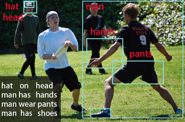
Scene graph generation is a sophisticated task because there is no specific recognition pattern (e.g., looking at and near have no conspicuous difference concerning vision, whereas near could occur between entities with different morphology ). Thus some scene graph generation methods are trapped into most frequent relation predictions caused by capricious visual features and trivial dataset annotations. Therefore, recent works emphasized the “unbiased” approaches to balance predictions for a more informative scene graph. However, human’s quick and accurate judgments over relations between numerous objects should be attributed to bias (i.e., experience and linguistic knowledge) rather than pure vision. To enhance the model capability, inspired by the “cognitive bias” mechanism, we propose a novel 3-paradigms framework that simulates how humans incorporate the label linguistic features as guidance of vision-based representations to better mine hidden relation patterns and alleviate noisy visual propagation. Our framework is model-agnostic to any scene graph model. Comprehensive experiments prove our framework outperforms baseline modules in several metrics with minimum parameters increment and achieves new SOTA performance on Visual Genome dataset.
1 Introduction
Scene graph generation refers to the vision task that detects objects and recognizes semantic relationships between different objects in an image. With graph-based representation, we could depict the semantic content of images in a structural and efficient way. Such a structural representation of images could greatly benefit downstream vision tasks, including image captioning[7][36], visual question answering [42][25][29], and video understanding[30].
However, the application of scene graph is confined by full of low semantic predictions in previous scene graph models. The inferior predictions is a consequence of several factors. First, the relationship sample distributions in existing representative datasets are long-tailed. For example, the sum of relations on,in, of in the widely adopted Visual Genome dataset[11] counts for more than 50% of the total (Figure.1a). Therefore the network shows a strong tendency to head relations and behaves poor on most tail classes. Besides, the image annotation is incomplete. Those informative but distant relations are typically ignored and thus falsely treated as negative samples during learning. As shown in Figure1b, Second, those tail relations (i.e., play, see) typically involve complex semantic meaning and large intra-class variations in images. Large intra-class variations combined with few samples make feature representation learning hard for those tail relations.
To address the aforementioned challenges, a large number of studies have been conducted to enhance quality of predictions. Concerning long-tailed data distribution issue, recent works strive for designing “debiased” methods, which re-design inference procedures or loss functions to obtain a balance prediction. Nonetheless, these “debiased” methods could be seen as a special form of “re-weighting” but in a learnable way. As no extra feature enhancement modules are introduced, these methods improve predictions on tail categories at the expense of those head categories. As for better feature representation learning, different propagation mechanisms have been developed for modeling context[12]. Nevertheless, it fails to achieve satisfactory performances due to noisy propagation.

However, bias should not be alleviated arbitrarily. In human recognition pipeline, “Cognitive bias”[32], as a psychological activity, benefits our decision-making in uncertain and intricate circumstances with the help of language[31]. Figure2 illustrates how cognitive bias impacts on relation cognition. Given a ball and woman entities, human first exploits experience of several most frequent occurrence relations between “ball” and “woman”, these candidates are served as the alternative choices for later decisions . Next, due to the experience can not represent the current circumstance, more precise guesses can be obtained by focusing on the part that woman contact the ball, which is the typical criteria when determines the relation between a person and a object. Noticed that the criteria is not necessary to be intersection part of two entities, but affected by categories. In the end, by considering all objects in this scene, it is not hard to conclude a shopping scenario. Hence human can choose “hold” as best choice by alleviating univocal meaning of “ball” with restriction “selling”.
In this work, inspired by three cognitive bias paradigms, we propose a language-based framework to enhance feature representations and reduce visual feature redundancy , by extracting prior knowledge of experience, linguistic local and global context respectively. Concretely, We first utilize object pair labels to simulate the experience over predicates to same space of prediction likelihoods in a supervised manner. Then, a language map module projects linguistic similarity as a channel-wised attention which focusing on local specific visual patterns that can impact final decisions. Moreover, a scene extractor module refines each object’s linguistic representation by the global context. To our best knowledge, we are the first to introduce human cognitive bias in Scene graph generation task, and utilize labels as high dimension representations. We conduct widely and detailed experiments on Visual Genome Dataset to prove framework effectiveness. The main contributions include:
- 1.
We propose a 3-paradigms cognitive bias framework that simulates human thinking procedure to effectively extracting informative relation patterns from images and remedy the trivial dataset problem.
- 2.
we design 3 cognition-driven language feature representations as the guidance of visual-based message propagation in the form of bias.
- 3.

2 Related Work
Scene Graph Generation: In the community, there are mainly three mainstream methods for scene graph generation. Early works widely adapted message passing between all object proposals[4][16][33][34][13][18], or aggregating within different type nodes[14]. This method commonly focused on the global context. A number of them[41][14] harnessed sequential memory model(LSTM[9] or GRU[3]), but failed to adopt edge feature in context formulation. Later works[12][26][38] harness Graph neural network(GCN[10]) processing node and edge features respectively, and focusing more on pair-wise information.[12] applied a multi-stage graph message propagation between proposal entities and relationship representation. In [38], Yang et al. pruned graph connections to sparse one, then attentional graph convolution network is applied for modulating information flow. [26] utilized GCN for updating state representations as energy value. Chen et al.[1] constructed a graph between proposal and all relationship representations and aggregated messages by GRU. Yet, those works suffered from the drawback that GCN only propagates features on local context deteriorates model to draw dominant predicates, which was addressed by[27] as biased training. Aiming to fix this shortcoming, recent works proposed novel pipeline and utilized prior knowledge [27][17][37][5][2][6]. serving as a plugin to generalized scene graph model.
Prior Knowledge: Current works addressed the fundamental role of prior knowledge in terms of the long-tail problem. The commonly adopted method is leveraging statistical results[41] as addictions on the decision layer. For instance, “FREQ”[41] directly summed prior distribution to model decision layer by counting “subject-relation-object” co-occurrence in dataset. However, the counting approach is hard to mimic real word distribution because of low-quality annotations in datasets. Therefore, an increased number of works strived for leveraging prior knowledge in perception procedure. [19] designed a language module, which concatenated two retrained word vectors and projected representation to the same space of vision module for minimizing the distance of similar semantic features. [24] entangled the perception and prior in a single model with shared parameters trained by multi-task learning. [28] introduced a confidence estimation module to alleviate the error propagation by incorporating confidence estimation in graph node feature updating. [39] incorporated external commonsense knowledge by unifying the formulation of scene graph and commonsense graph [1] incorporates co-occurrence of objects and relations to form a knowledge graph as a constraint in graph message propagation. [40] structured visual commonsense and proposed a cascaded fusion architecture for fusion. Our model combines both the decision layer and the feature processing layer’s fusion.
Scene Graph Debasing: Due to the lang-tail problems, some researchers proposed the ”unbiased” concept, which prevents model overfitting to most frequent categories. Early works simply adopted weighted loss or focal loss[15] for balanced prediction. Later, Yan et al.[37] designed a training scheme that loss weight is dynamically changed based on predicate’s visual feature similarity, which is learned by minimizing the distance of similar predicate features. Nonetheless, vision patterns of relations are highly fickle, hence hard to learn. [27] presented a general unbiased inference pipeline that utilized Total Direct Effect analysis. However, this approach did not enrich model capability, but also wiped out object labels information, which can bring out beneficial language cues. On the contrary, our approach exhaustively uses labels for assisting vision. Experiments in 4.3 support our hypothesis.

3 Methodology
3.1 Problem Formulation
Given an image , scene graph generation task aims to predict object coordinates (bounding box) , classes as well as relation between objects. The task can further denote as the optimization of . For a graph structure, it normally consists of nodes and edges. We denote as i-th object representation. as edge representation from node to ,
3.2 Framework Architecture
Our proposed cognition bias (C-bias) framework overall architecture is presented in Figure3a, which is consist of three paradigms. 1) the experience estimation module is to draw the relation distribution on supervision of joint possibility. This distribution is added on final model outputs. 2) the language map module (Figure3b) is to learn local interactions between pair labels and produce channel-wised attention for visual features. 3) the scene extractor module (Figure3c) is to globally consider the linguistic context in an image, and then update the initial label embedding. Those three sub-modules construct an enhanced graph representation by introducing label features in the vision-based baseline model at the output, edge, node, respectively.
3.2.1 Object Detection Network:
Concretely, given an image, a pre-trained object detection network is used to obtain a predicted object location set and a class set with number . Detection network can be written as:
| (1) |
where is an input image.
3.2.2 Paradigm 1: Experience Estimation Module:
This module learns the joint likelihood of two objects over relationships. We expect it can output distributions that base on the experience of correlation between predicates and categories. The estimated experience can be acquired by MLP layers, with the input of pair label categories and position embedding . Here, we use different weight and to transform subject and object labels to their linguistic representations, respectively. The predicted distribution between -th subject and -th object can be describe as:
| (2) | ||||
| (3) |
Where are object coordination, width, height. are fully connect layer with activation function (e.g. RELU). is concatnation operation.
Here, unlike previous “FREQ”[41] method that directly counts triblets co-occurrence frequency as prediction likelihood weights, we utilize the joint possibility as supervision signals to obtain a comprehensive and accurate relation distribution over tail categories. Suppose the dataset contains number of object categories and relation categories, the joint possibility of subject i with object j is denoted as:
| (4) |


Where are statistical marginal distribution of subject and object categories over relation categories (e.g., Figure4). Compare to directly counting number of triblet combinations, marginal distribution does not suffer a lot from sample scarcity, thus can generate more accurate distribution. Noticed that the relation distribution of the same object classes is alternated depending on whether it serves as a subject or object. For instance, Figure4a shows that “man” as the subject is possible having correlation with “eating”. Inversely, in Figure4b, it is impossible.
Finally, For learning distribution purpose, we choose cosine loss function between target and predicted prediction , which is denoted as:
| (5) |
3.2.3 Paradigm 2: Language Map Module:
To incorporate the language feature with local linguistic context into visual feature, we design a “language mapping” (LM) operation to generate linguistic attention based on label pairs and project it to the same dimensions as the edge (conventionally, it is the visual feature of union area). Say we got two predicted class labels and , the initial language map is produced by the vector multiplication as follows:
| (6) |
Where , are word embedding weights of subjects and objects. is dot product operation. The language map initially can be regarded as a covariance matrix between subject and object word embeddings, which contains informative correlation information. Then, pooling and 2D-convolution are applied to gain channel-wised linguistic attention. The language map feature can be denoted as Eq.7.
3.2.4 Paradigm 3: Scene Extractor Module
The aforementioned paradigms both generate deterministic linguistic representations given the input label pair. However, the same word in different contexts could have different semantic meanings. Hence, the purpose of this module is to extract global semantics context into each category representation. Hence we leverage multi-head self-attention to achieve that. Differing from prior work[20] taking visual object features as transformer input, this module only takes object labels concatenated with positions for context encoding. Specifically, our module consists of several stacked multi-head attention layers with a Feed Forward network (FF) to update each node (object) feature. Given an image, suppose there are object proposals that are packed together as input .
| (10) |
Where is object’s label embedding weights and is position embedding of i-th proposal as the same formulation as Eq.2. is concatenation operation. Then attention mechanism can be written as:
| (11) |
Where refer to query, key, value respectively, corresponding to parameter matrices, is the dimension of key. So we formulate multi-head attention as:
| (12) | ||||
| (13) |
Where is a MLP layer with the purpose of merging all attention heads. Finally, scene representation of i-th object can be described as:
| (14) | ||||
| (15) |
Where is output of multi-head attention. are FPN parameter matrices and biases. Then the -th node feature is updated:
| (16) |
Where is concatenation operator.
3.2.5 Baseline Model
After edge and object features are updated, any off-the-shelf scene graph generation network can be used. It could be either a message propagating method or a graph neural network, as long as it exerts node or edge features for prediction. This network can be described as:
| (17) |
Where is a given image, Object location set, class set. and are node and edge features enhanced by language. Then, SGG model output and ”Paradigm 1” estimated relation distribution are collectively considered:
| (18) |
4 Experiments
In this section, we first introduce the dataset and evaluation metrics we used as well as the implementation details. Then the comprehensive comparison experiments with other scene graph methods and ablation studies on three paradigms are conducted. Finally, we demonstrate quantitative results for illustration purposes.
4.1 Evaluation Protocol
Datasets: We train and evaluate on filtered Visual Genome split VG150
proposed in[35] to keep consistency with other studies. The VG150 dataset
contains the most frequent 150 objects and 50 relationships with 108k images,
in which 70% images are held out for training and 30% for testing. Among the
training set, 5000 images are fetched for evaluation.
Tasks: 1) predicate classification (PredCls) task
predicts predicates given the ground truth locations and classes. 2)
scene graph classification (SGCls) task recognizes predicates and
classes given locations. scene graph generation (SGGen) predicts
valid objects (IoU 0.5) and classes as well as predicates.
4.2 Implementation Details
All models are training on two NVIDIA Titan XP GPUs. The learning scheduler is
WarmupReduceLROnPlateau with decay factor 0.6 and patient 6. The base learning
rate is 0.08,0.08,0.06, and batch size is 12. We choose the SGD optimizer for
optimization.
Detector: We use pretrained faster-rcnn[23] with
backbone ResNeXt-101-FPN[8] . We froze its weights during training.
C-bias Framework: We test BGNN[12], Motifs[41] and G-RCNN[38] as baseline. For a fair comparison, all configurations in our proposed network will be identical to baseline settings, including node and edge feature dimensions. Noticed that for each baseline model, we choose the same configurations for all 3 tasks. We use pre-trained glove.6B[22] with as the initial word embedding weights , for three paradigms. Specifically, for paradigm 1, we use 3 FC layers with 1024 neurons and is a 2 layers MLP with hidden dimension 4096. For paradigm 2, We choose two convolution layers to generate a 256-channels language feature map. The output size of ROIAlign[8] is 77. For paradigm 3, We use 4 layers self-attention with 8 heads, of which output 512-dim linguistic-based object features .
| Model | Method | PredCls | SGCls | SGGen | |||||||
| mR@20 | mR@50 | mR@100 | mR@20 | mR@50 | mR@100 | mR@20 | mR@50 | mR@100 | |||
| constraint | PCPL*[37] | / | / | 35.2 | 37.8 | / | 18.6 | 19.6 | / | 9.5 | 11.7 |
| IMP*[35] | / | / | 15.8 | 17.2 | / | 9.3 | 9.6 | / | 6.0 | 7.3 | |
| VCTree*[28] | / | / | 15.4 | 16.6 | / | 7.4 | 7.9 | / | 8.2 | 9.7 | |
| G-RCNN[38] | baseline | 13.21 | 16.46 | 17.28 | 8.35 | 9.67 | 10.17 | 3.45 | 4.89 | 5.95 | |
| C-bias | 15.75 | 18.64 | 19.80 | 8.62 | 10.11 | 10.8 | 3.80 | 5.15 | 6.24 | ||
| Motifs[41] | baseline | 16.26 | 18.79 | 19.69 | 7.90 | 9.39 | 9.97 | 3.53 | 5.22 | 6.65 | |
| C-bias | 16.61 | 20.38 | 21.87 | 8.50 | 9.89 | 10.41 | 3.91 | 5.49 | 6.99 | ||
| BGNN[12] | baseline | 26.21 | 30.64 | 32.76 | 13.24 | 15.58 | 16.58 | 7.82 | 10.59 | 12.75 | |
| C-bias | 31.30 | 36.31 | 38.44 | 15.80 | 20.38 | 21.87 | 11.63 | 14.43 | 17.24 | ||
| no constraint | PCPL* | / | / | 50.6 | 62.6 | / | 26.8 | 32.8 | / | 10.4 | 14.4 |
| IMP* | / | / | 9.8 | 10.5 | / | 5.8 | 6.0 | / | 3.8 | 4.8 | |
| G-RCNN | baseline | 21.66 | 35.74 | 46.02 | 13.66 | 20.11 | 24.71 | 4.04 | 6.62 | 10.11 | |
| C-bias | 23.31 | 36.38 | 46.45 | 13.83 | 20.77 | 26.23 | 4.03 | 6.66 | 10.27 | ||
| Motifs | baseline | 23.12 | 35.90 | 47.72 | 12.90 | 19.76 | 25.54 | 4.31 | 7.37 | 10.72 | |
| C-bias | 23.95 | 37.12 | 49.67 | 13.59 | 20.73 | 26.08 | 4.59 | 7.57 | 11.55 | ||
| BGNN | baseline | 34.41 | 49.02 | 61.04 | 17.96 | 25.29 | 30.98 | 8.66 | 13.63 | 17.97 | |
| C-bias | 36.94 | 51.20 | 63.02 | 20.10 | 28.01 | 33.65 | 13.57 | 17.07 | 21.98 | ||
4.3 Quantitative Results
Mean Recall: Table 1 shows comparisons between
various methods and our C-bias framework on constrained mean recall(mR@K) on VG
dataset. We notice a consistent improvement on mR@K on all baseline models. By
plugging our framework in BGNN, our framework surpasses prior SOTA performance
in three tasks yielded by [37] and[12] (mR@100: 37.8%, 16.6%,
12.8% ). It is attributed to valid local and global language representation
merging paradigms. To compare with baseline BGNN[12], our framework
gains relative improvements of 17.3% , 31.9% and 35.2% on mean recall@100
metrics. The mR@K improvement should attribute to enhanced feature powered by
language’s generalization and invariability capability, which reduces noisy
propagation between nodes and edges, therefore, elevates tail relation
predictions.
In terms of Motifs and G-RCNN, relatively minor improvements are obtained from
3 tasks over mR@k. It may caused by lack of pair-wise edge feature (e.g., union
features) utilization, In consequence, the second paradigms can only be
applied to the last perception layer, leading to poor performance gain.
However, we find that some wrong predictions of our framework are more accurate
than annotations, which is elaborated in Section4.7.
No-graph Constraint Mean Recall: Table 1 also
reports no graph constraint mean recall(ng-mR) performance on the VG dataset,
which reveals consistent superior results on baseline models. With baseline
BGNN,ng-mR@100 increases 3.2%, 8.6%, 22.31%. Results reflects our
framework’s capability of predicting correct predicates with higher confidence
when there is no graph constraint.
Zero-shot Recall: We also measure zero-shot recall (zR@K) for evaluating the framework generalization capability, results are shown in Table2. In each task, our framework still has noticeable improvements in PredCls tasks, with relative improvement 16.37%, 5.72%, 33.4% on zR@100 in 3 baselines, due to available of ground truth labels. However, the training process shows a relatively contradictory tendency between mR@K and zR@K performance, revealing that those subject-predicate-object combinations that do not occur in the training set have a considerable proportion of high-frequency predicates. Limited by length of paper, more experiments would be posted on supplement materials.
| Model | Method | PredCls | SGCls | SGGen | |||
|---|---|---|---|---|---|---|---|
| zR@50 | zR@100 | zR@50 | zR@100 | zR@50 | zR@100 | ||
| G-RCNN | baseline | 10.22 | 12.22 | 6.67 | 7.56 | 0.44 | 0.44 |
| C-bias | 12.44 | 14.22 | 4.67 | 6.44 | 0.44 | 0.44 | |
| MOTIFS | baseline | 10.22 | 11.70 | 6.22 | 6.22 | 0.00 | 0.00 |
| C-bias | 10.44 | 12.37 | 5.33 | 6.67 | 0.00 | 0.22 | |
| BGNN | baseline | 4.44 | 5.33 | 3.56 | 3.56 | 0.44 | 0.44 |
| C-bias | 6.22 | 7.11 | 3.56 | 4.0 | 0.00 | 1.33 | |
4.4 Predicate Analyze:
Shown in Figure5, we present each predicate category’s mR@100 performance on PredCls task. Among which yellow pillars represent Baseline BGNN, whereas blue ones represent the proposed C-bias framework. Even compared with such a strong baseline model, We still notice more precise predictions that our framework gets, from which 44 of predicates are better recalled by our framework. Besides, there are predicates that the baseline model fails to recall (e.g.across, against, growing on, mounted on, says, walking in, etc.) been successfully hit by the proposed C-bias framework, which supports the claim that our framework successfully inducts relation patterns between objects.

4.5 Ablation Studies
To reveal the effectiveness of each paradigm, we incrementally add them to the
baseline one by one. For simplicity, we choose BGNN as the baseline for
illustration. The results are shown in Table.3.
Paradigm1:We observe that adding the Experience estimation
module improves baseline with 6.83%, 15.07%, 32.70% over three tasks on
mR@100 respectively, which accounts for relation distribution learned from
supervision of joint distribution. Besides, compared with the baseline that
using FREQ[41], results prove the hypothesis that joint possibility
indeed describes real-world distribution more precisely.
Paradigm2: Furthermore, the Language map module promotes the
performance to 37.68, 19.82, 17.15. Noticed that the gap between mR@50 and
mR@100 shrinks, indicating a lower false prediction proportion in top guesses.
It is expected that channel-wised language map effectively guides union visual
feature finding intrinsic object-relation patterns, which in turn leads to the
confidence of positive-true predictions boosting.
| Model | PredCls | SGCls | SGGen | |||
|---|---|---|---|---|---|---|
| mR@50 | mR@100 | mR@50 | mR@100 | mR@50 | mR@100 | |
| BGNN | 30.40 | 32.76 | 14.30 | 16.58 | 10.70 | 12.75 |
| BGNN+EEM | 32.75 | 35.00 | 17.77 | 19.08 | 14.54 | 16.92 |
| BGNN+EEM+LMM | 35.99 | 37.68 | 18.71 | 19.82 | 15.10 | 17.15 |
| BGNN+EEM+LMM+SEM | 36.31 | 38.44 | 20.38 | 21.87 | 14.43 | 17.24 |
Paradigm3: By adding the Scene extractor module, the performances further reach 38.44, 20.87, and 17.24. Through SEM brings a relatively tiny improvement than other modules, it meets our anticipation that global language context mainly serves as the assistance when a label is ambiguous.
4.6 Model Size and Runtime:
We present several model parameters and inference time in Table4. We choose BGNN and MOTIFS as baselines, C-bias and Unbiased[27] as a plug-in model. Though Unbiased is claimed as a inference method, our framework still shows low computational requirements than Unbiased. For C-bias, parameters of model merely increased 5.33% and 6.17% in two baselines, the performance of mean recall@100 increases 24.88% and 8%, Compare with unbiased, our framework size is smaller but perform better. This advantage comes from label input of 3 paradigms, which is low-dimensional than image.
| Model | BGNN | BGNN+Ours | BGNN+Unbiased | MOTIFS | MOTIFS+Ours |
|---|---|---|---|---|---|
| Params | 341.9M | 360.13M | 365.746M | 367.17M | 389.82M |
| Relative increase | / | 5.33% | 6.98% | / | 6.17% |
| Inference Time(ms) | 497.5 | 538.1 | 539.2 | 420.4 | 450.9 |
| Mean recall@100 | 32.76 | 38.44 | 34.89 | 6.65 | 6.99 |

4.7 Qualitative Studies
Beyond numbers, we emphasize the intuitive evaluation because trivial and uncompleted ground truth has traumatized the authority of metrics. Some inspiring findings that we discovered from wrong results of SGGen task in Figure6 reveal several advantages that the C-bias framework has over baseline and annotations, including:
- 1.
Multi-scaled: An intuitive sensation is that our results generate more relations widespread in the whole scene. Compared to baseline results which are incapable of detecting relations with no overlaps, our C-bias framework successfully recognizes distanced entities’ correlations. In Figure 6, the last column of first image shows our framework can notice man walk on sidewalk in a small area of the background.
- 2.
Accurate and Informative: The baseline predicts multitudinous less meaningful categories ”on, in, of”. We speculate that it is caused by massive repeated annotations full in annotations (ground truth graph in the first row of Figure 6), which indeed deteriorate model learning. Intuitively, we find that our proposed framework can mine meaningful but inconspicuous correlations regardless of trivial annotations. Take last row of Figure6 for example, ”letter” are neither part of annotations or baseline results, and logo on bus in annotations is not informative. Inspiringly, in the C-bias framework, relation triblets letter painted on bus and logo mounted on bus are more accurate.
5 Conclusion
In this paper, we propose a novel cognitive bias framework in SGG task to properly mining fickle relation patterns by incorporating local, global context with help of linguistics information. We simulate human cognitive bias paradigms to acquire better relation perception capability, and address crucial role of using label-derivative linguistic features as biases upon visual message propagation. The result shows superiority over previous works.
References
- [1] Chen, T., Yu, W., Chen, R., Lin, L.: Knowledge-embedded routing network for scene graph generation. In: Proceedings of the IEEE/CVF Conference on Computer Vision and Pattern Recognition. pp. 6163–6171 (2019)
- [2] Chiou, M.J., Ding, H., Yan, H., Wang, C., Zimmermann, R., Feng, J.: Recovering the unbiased scene graphs from the biased ones. In: Proceedings of the 29th ACM International Conference on Multimedia. pp. 1581–1590 (2021)
- [3] Cho, K., Van Merriënboer, B., Gulcehre, C., Bahdanau, D., Bougares, F., Schwenk, H., Bengio, Y.: Learning phrase representations using rnn encoder-decoder for statistical machine translation. arXiv preprint arXiv:1406.1078 (2014)
- [4] Dai, B., Zhang, Y., Lin, D.: Detecting visual relationships with deep relational networks. In: Proceedings of the IEEE conference on computer vision and Pattern recognition. pp. 3076–3086 (2017)
- [5] Garg, S., Dhamo, H., Farshad, A., Musatian, S., Navab, N., Tombari, F.: Unconditional scene graph generation. In: Proceedings of the IEEE/CVF International Conference on Computer Vision. pp. 16362–16371 (2021)
- [6] Gkanatsios, N., Pitsikalis, V., Koutras, P., Maragos, P.: Attention-translation-relation network for scalable scene graph generation. In: Proceedings of the IEEE/CVF International Conference on Computer Vision Workshops. pp. 0–0 (2019)
- [7] Gu, J., Joty, S., Cai, J., Zhao, H., Yang, X., Wang, G.: Unpaired image captioning via scene graph alignments. In: Proceedings of the IEEE/CVF International Conference on Computer Vision. pp. 10323–10332 (2019)
- [8] He, K., Gkioxari, G., Dollár, P., Girshick, R.: Mask r-cnn. In: Proceedings of the IEEE international conference on computer vision. pp. 2961–2969 (2017)
- [9] Hochreiter, S., Schmidhuber, J.: Long short-term memory. Neural computation 9(8), 1735–1780 (1997)
- [10] Kipf, T.N., Welling, M.: Semi-supervised classification with graph convolutional networks. arXiv preprint arXiv:1609.02907 (2016)
- [11] Krishna, R., Zhu, Y., Groth, O., Johnson, J., Hata, K., Kravitz, J., Chen, S., Kalantidis, Y., Li, L.J., Shamma, D.A., et al.: Visual genome: Connecting language and vision using crowdsourced dense image annotations. International journal of computer vision 123(1), 32–73 (2017)
- [12] Li, R., Zhang, S., Wan, B., He, X.: Bipartite graph network with adaptive message passing for unbiased scene graph generation. In: Proceedings of the IEEE/CVF Conference on Computer Vision and Pattern Recognition (CVPR). pp. 11109–11119 (June 2021)
- [13] Li, Y., Ouyang, W., Zhou, B., Shi, J., Zhang, C., Wang, X.: Factorizable net: an efficient subgraph-based framework for scene graph generation. In: Proceedings of the European Conference on Computer Vision (ECCV). pp. 335–351 (2018)
- [14] Li, Y., Ouyang, W., Zhou, B., Wang, K., Wang, X.: Scene graph generation from objects, phrases and region captions. In: Proceedings of the IEEE international conference on computer vision. pp. 1261–1270 (2017)
- [15] Lin, T.Y., Goyal, P., Girshick, R., He, K., Dollár, P.: Focal loss for dense object detection. In: Proceedings of the IEEE international conference on computer vision. pp. 2980–2988 (2017)
- [16] Lin, X., Ding, C., Zeng, J., Tao, D.: Gps-net: Graph property sensing network for scene graph generation. In: Proceedings of the IEEE/CVF Conference on Computer Vision and Pattern Recognition. pp. 3746–3753 (2020)
- [17] Liu, H., Yan, N., Mortazavi, M., Bhanu, B.: Fully convolutional scene graph generation. In: Proceedings of the IEEE/CVF Conference on Computer Vision and Pattern Recognition. pp. 11546–11556 (2021)
- [18] Liu, Y., Wang, R., Shan, S., Chen, X.: Structure inference net: Object detection using scene-level context and instance-level relationships. In: Proceedings of the IEEE conference on computer vision and pattern recognition. pp. 6985–6994 (2018)
- [19] Lu, C., Krishna, R., Bernstein, M., Fei-Fei, L.: Visual relationship detection with language priors. In: European conference on computer vision. pp. 852–869. Springer (2016)
- [20] Lu, Y., Rai, H., Chang, J., Knyazev, B., Yu, G., Shekhar, S., Taylor, G.W., Volkovs, M.: Context-aware scene graph generation with seq2seq transformers. In: Proceedings of the IEEE/CVF International Conference on Computer Vision. pp. 15931–15941 (2021)
- [21] Newell, A., Deng, J.: Pixels to graphs by associative embedding. Advances in neural information processing systems 30 (2017)
- [22] Pennington, J., Socher, R., Manning, C.D.: Glove: Global vectors for word representation. In: Proceedings of the 2014 conference on empirical methods in natural language processing (EMNLP). pp. 1532–1543 (2014)
- [23] Ren, S., He, K., Girshick, R., Sun, J.: Faster r-cnn: Towards real-time object detection with region proposal networks. Advances in neural information processing systems 28 (2015)
- [24] Sharifzadeh, S., Baharlou, S.M., Tresp, V.: Classification by attention: Scene graph classification with prior knowledge. arXiv preprint arXiv:2011.10084 (2020)
- [25] Shi, J., Zhang, H., Li, J.: Explainable and explicit visual reasoning over scene graphs. In: Proceedings of the IEEE/CVF Conference on Computer Vision and Pattern Recognition. pp. 8376–8384 (2019)
- [26] Suhail, M., Mittal, A., Siddiquie, B., Broaddus, C., Eledath, J., Medioni, G., Sigal, L.: Energy-based learning for scene graph generation. In: Proceedings of the IEEE/CVF Conference on Computer Vision and Pattern Recognition. pp. 13936–13945 (2021)
- [27] Tang, K., Niu, Y., Huang, J., Shi, J., Zhang, H.: Unbiased scene graph generation from biased training. In: Proceedings of the IEEE/CVF Conference on Computer Vision and Pattern Recognition. pp. 3716–3725 (2020)
- [28] Tang, K., Zhang, H., Wu, B., Luo, W., Liu, W.: Learning to compose dynamic tree structures for visual contexts. In: Proceedings of the IEEE/CVF conference on computer vision and pattern recognition. pp. 6619–6628 (2019)
- [29] Teney, D., Liu, L., van Den Hengel, A.: Graph-structured representations for visual question answering. In: Proceedings of the IEEE conference on computer vision and pattern recognition. pp. 1–9 (2017)
- [30] Teng, Y., Wang, L., Li, Z., Wu, G.: Target adaptive context aggregation for video scene graph generation. In: Proceedings of the IEEE/CVF International Conference on Computer Vision. pp. 13688–13697 (2021)
- [31] Tobeña, A., Marks, I.M., Dar, R.: Advantages of bias and prejudice: an exploration of their neurocognitive templates. Neuroscience & Biobehavioral Reviews 23, 1047–1058 (1999)
- [32] Tversky, A., Kahneman, D.: Judgment under uncertainty: Heuristics and biases: Biases in judgments reveal some heuristics of thinking under uncertainty. science 185(4157), 1124–1131 (1974)
- [33] Wang, W., Wang, R., Shan, S., Chen, X.: Exploring context and visual pattern of relationship for scene graph generation. In: Proceedings of the IEEE/CVF Conference on Computer Vision and Pattern Recognition (CVPR) (June 2019)
- [34] Woo, S., Kim, D., Cho, D., Kweon, I.S.: Linknet: Relational embedding for scene graph. Advances in Neural Information Processing Systems 31 (2018)
- [35] Xu, D., Zhu, Y., Choy, C.B., Fei-Fei, L.: Scene graph generation by iterative message passing. In: Proceedings of the IEEE conference on computer vision and pattern recognition. pp. 5410–5419 (2017)
- [36] Xu, N., Liu, A.A., Liu, J., Nie, W., Su, Y.: Scene graph captioner: Image captioning based on structural visual representation. Journal of Visual Communication and Image Representation 58, 477–485 (2019)
- [37] Yan, S., Shen, C., Jin, Z., Huang, J., Jiang, R., Chen, Y., Hua, X.S.: Pcpl: Predicate-correlation perception learning for unbiased scene graph generation. In: Proceedings of the 28th ACM International Conference on Multimedia. pp. 265–273 (2020)
- [38] Yang, J., Lu, J., Lee, S., Batra, D., Parikh, D.: Graph r-cnn for scene graph generation. In: Proceedings of the European conference on computer vision (ECCV). pp. 670–685 (2018)
- [39] Zareian, A., Karaman, S., Chang, S.F.: Bridging knowledge graphs to generate scene graphs. In: European Conference on Computer Vision. pp. 606–623. Springer (2020)
- [40] Zareian, A., Wang, Z., You, H., Chang, S.F.: Learning visual commonsense for robust scene graph generation. In: European Conference on Computer Vision. pp. 642–657. Springer (2020)
- [41] Zellers, R., Yatskar, M., Thomson, S., Choi, Y.: Neural motifs: Scene graph parsing with global context. In: Proceedings of the IEEE Conference on Computer Vision and Pattern Recognition. pp. 5831–5840 (2018)
- [42] Zhang, C., Chao, W.L., Xuan, D.: An empirical study on leveraging scene graphs for visual question answering. arXiv preprint arXiv:1907.12133 (2019)