Sensitivity analysis in longitudinal clinical trials via distributional imputation
Abstract
Missing data is inevitable in longitudinal clinical trials. Conventionally, the missing at random assumption is assumed to handle missingness, which however is unverifiable empirically. Thus, sensitivity analysis is critically important to assess the robustness of the study conclusions against untestable assumptions. Toward this end, regulatory agencies often request using imputation models such as return-to-baseline, control-based, and washout imputation. Multiple imputation is popular in sensitivity analysis; however, it may be inefficient and result in an unsatisfying interval estimation by Rubin’s combining rule. We propose distributional imputation (DI) in sensitivity analysis, which imputes each missing value by samples from its target imputation model given the observed data. Drawn on the idea of Monte Carlo integration, the DI estimator solves the mean estimating equations of the imputed dataset. It is fully efficient with theoretical guarantees. Moreover, we propose weighted bootstrap to obtain a consistent variance estimator, taking into account the variabilities due to model parameter estimation and target parameter estimation. The finite-sample performance of DI inference is assessed in the simulation study. We apply the proposed framework to an antidepressant longitudinal clinical trial involving missing data to investigate the robustness of the treatment effect. Our proposed DI approach detects a statistically significant treatment effect in both the primary analysis and sensitivity analysis under certain prespecified sensitivity models in terms of the average treatment effect, the risk difference, and the quantile treatment effect in lower quantiles of the response, uncovering the benefit of the test drug for curing depression.
keywords: Longitudinal clinical trial, missing data, distributional imputation, multiple imputation, sensitivity analysis
1Department of Statistics, North Carolina State University, Raleigh, NC, USA
2Merck & Co., Inc., Kenilworth, NJ, USA
1 Introduction
In longitudinal clinical trials, participants are likely to deviate from the protocol that causes the missing data. The deviations from the protocol may include poor compliance with the treatment or loss of follow-ups. Rubin 1976 develops a framework to handle missingness in data. Three missing mechanisms have been proposed as missing completely at random (MCAR), missing at random (MAR), and missing not at random (MNAR). Missingness that is not related to any components of the data, e.g., participants dropping out of the trial due to work or family considerations, is categorized as MCAR. While in most clinical studies involving patients with missing outcomes, it is likely that the missingness depends on the health status of patients. For example, individuals with severe outcomes are more likely to drop out from the study or switch to certain rescue therapies. MAR is typically used in longitudinal clinical trials targeting the primary analysis, which assumes that the conditional outcome distribution stays the same between the participants who remain in the study and the ones who drop out, i.e., the participants are assumed to take the assigned treatment even after the occurrence of missingness. However, the MAR assumption is not verifiable and may be violated for some drugs with a short half-life, where the treatment effect quickly fades away once the individuals discontinue from the active treatment, leading to a missing not at random (MNAR) assumption. Therefore, it is vital to conduct sensitivity analyses to explore the robustness of results to alternative MNAR-related assumptions as recommended by the US Food and Drug Administration (FDA) and National Research Council (Little et al. 2012).
The importance of defining an appropriate treatment effect estimand in the presence of missing data has been put forward by the ICH E9(R1) working group. Following the instructions in ICH 2021, the estimand should give a precise description of the treatment effect of interest from a population perspective, and account for the intercurrent events such as the discontinuation of treatment. In the primary analysis of the treatment effect estimand, we can assume MAR under an envisioned condition that participants with the treatment discontinuation still follow the assigned therapy throughout the study (Carpenter et al. 2013). For sensitivity or supplemental analyses, we evaluate the treatment effect under scenarios that deviate from MAR and call these settings sensitivity analyses for simplicity throughout the paper.
In sensitivity analyses, we consider several plausible missingness scenarios under MNAR based on the pattern-mixture model (PMM; Little 1993) framework, which we call the “sensitivity models”. Our main focus in this paper is on the jump-to-reference (J2R) scenario proposed by Carpenter et al. 2013, which assumes that the missing outcomes in both treatment groups will have the same distributional profile as those in the control group with the same covariates. We also briefly introduce other sensitivity models such as return-to-baseline (RTB) and washout imputation, which have been used in the FDA statistical review and evaluation reports for certain treatments (e.g., US Food and Drug Administration 2016). Although we focus on specific sensitivity models, our framework can be extended readily to other imputation mechanisms and the mixture of imputation strategies in sensitivity analyses.
To handle missingness in sensitivity analyses, the likelihood-based method and multiple imputation (MI) are the two most common approaches. The likelihood-based method typically utilizes the ignorability of the missing mechanism under MAR to draw valid maximum-likelihood inferences given variation independence, i.e., the parameters that control the missing mechanism and the model parameters are separable. For longitudinal clinical trials with continuous responses, one can fit a mixed model with repeated measures (MMRM) and incorporate the missing information to obtain inferences (e.g., Mehrotra et al. 2017; Zhang et al. 2020). While it is efficient, the analytical form for the likelihood-based method is only feasible to derive under restrictive scenarios such as normality or when we are dealing with mean types of estimands, and it requires rederivations if the missingness pattern changes. MI developed by Rubin 2004 resorts to using computational techniques to ease the analytical requirements from the likelihood-based method. The FDA and National Research Council (Little et al. 2012) highly recommend the use of MI and Rubin’s MI combining rules to get inferences due to its flexibility and simplicity. However, Wang and Robins 1998 reveal that the MI estimator is not efficient in general. Moreover, the inefficiency of MI can be more severe in terms of interval estimation, where the variance estimation using Rubin’s rule may not be consistent even when the imputation and analysis models are the same correctly specified (Robins and Wang 2000). In sensitivity analyses, overestimation of the variance using Rubin’s rule is commonly detected in literature (e.g., Lu 2014; Liu and Pang 2016; Yang and Kim 2016b). The motivating example in Section 2 further shows an alteration of the study conclusion due to the conservative variance estimator, where the same statistically significant treatment effect fails to be detected in the sensitivity analysis, rising a dilemma for the investigators in the process of decision-making. To overcome the problem, the variance estimation derived from the bootstrap approach is applied. But it is more computationally intensive than the traditional Rubin’s method since it requires the re-imputation of the missing components and the reconstruction of the imputation model per bootstrap iteration.
In this paper, we propose distributional imputation (DI) based on the idea of Monte Carlo (MC) integration (Lepage 1978) and develop a unified framework to conduct sensitivity analyses using DI in longitudinal clinical trials. The motivation of DI is to impute the missing components from the target imputation model given the observed data and use the mean estimating equations approximated by MC integration to draw efficient inferences. The implementation consists of three major steps: first, obtain the model parameter estimator based on the observed data; second, impute the missing values from the estimated sensitivity model; and third, derive the DI estimator of the parameter of interest by jointly evaluating the entire imputed dataset through mean estimating equations. We show that the DI estimator is consistent and asymptotically normal. We also propose a weighted bootstrap procedure for variance estimation, which incorporates the uncertainty from model parameter estimation and target parameter estimation. The DI estimator drawn from our framework is fully efficient with the firm theoretical ground. Moreover, the weighted-bootstrap variance estimator is consistent with straightforward realization and the avoidance of re-imputing the missing components compared to the conventional bootstrap methods. In the motivating example in Section 2, DI resolves the overestimation issue of Rubin’s combining rule under MI in the sensitivity analysis and detects a statistically significant benefit of using the test drug to cure depression. Our framework is applicable to a wide range of sensitivity models defined through estimating equations.
The rest of the paper proceeds as follows. Section 2 uses antidepressant clinical trial data to motivate the development of an efficient imputation method. Section 3 introduces the basic setup, provides notations, estimands, imputation mechanisms in sensitivity analyses, and comments on existing methods to handle missingness. Section 4 presents DI and its main steps. Section 5 gives the asymptotic theories for the DI estimator and proposes weighted bootstrap on variance estimation. Section 6 explores the finite-sample performance of the DI estimator via simulation. Section 7 returns to the motivating example and applies the proposed framework to the data. Section 8 draws the conclusion. Supplementary material contains the technical setup, proof of the theorems, and additional simulation and real-data application results.
2 Motivating example
An antidepressant clinical trial from the Auspices of the Drug Information Association is conducted to evaluate the effect of an experimental medication (Mallinckrodt et al. 2014). The study measures the longitudinal outcomes of the HAMD-17 score at baseline and weeks 1, 2, 4, 6, and 8 for 200 patients who are randomly assigned to the control and treatment groups at a 1:1 ratio. The data has a monotone missingness pattern except for one individual in the treatment group containing intermittent missingness. For illustration purposes, we assume MAR for this intermittent missingness and focus on the monotone missing data. To investigate the treatment effect in different aspects, we explore two population summaries by constructing different treatment effect estimands to evaluate the treatment effect. The first population-level summary is the average treatment effect (ATE) defined by the difference between the relative change of the HAMD-17 score from the baseline value in the last visit. The second population-level summary is the risk difference defined by the percentage difference of patients with or more improvement from the baseline HAMD-17 score at the last visit.
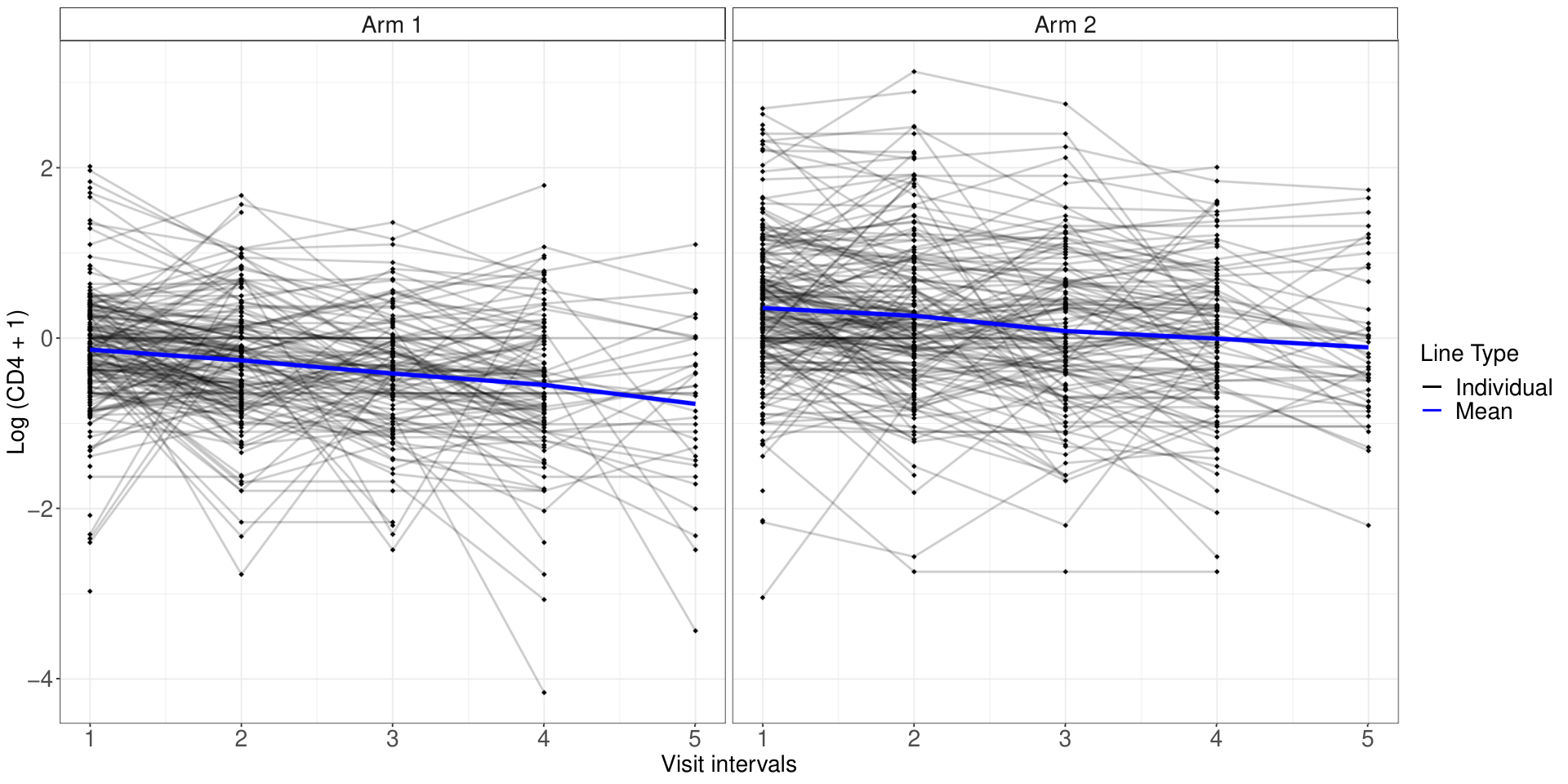
Figure 1 shows the spaghetti plot of the relative change of the HAMD-17 score for the two groups. It reflects a typical missing data issue in longitudinal clinical trials, with 39 patients in the control group and 30 patients in the treatment group dropping out during the study period. The relatively high dropout rate prompts the need for imputation to utilize the information related to the missingness.
As MI relies on the parametric modeling assumption, we begin by checking the normality of the conditional errors at each visit for model diagnosis. Figure 2 illustrates the normal Q-Q plots of the conditional residuals obtained by fitting the MMRM for the observed data. All the plots indicate an underlying normal distribution for the outcomes since the majority of residuals is within the confidence region, only the conditional errors at week 8 being slightly right-skewed.
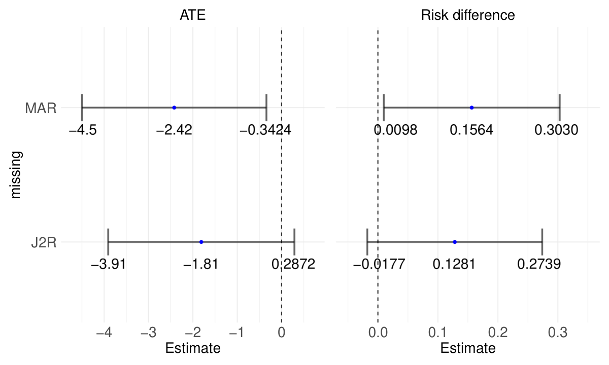
Under the normal assumption, we conduct MI to the missing components with the imputation size as under MAR to perform the primary analysis and under J2R for the sensitivity analysis to obtain the inferences using Rubin’s rule. The point estimates of the ATE and the risk difference accompanied with the CIs are presented in Figure 3. In the primary analysis that assumes MAR, both the ATE and the risk difference reveal a significant treatment effect. However, the sensitivity analysis under J2R fails to capture the same significance under MI, leading to a loss of the credibility of the experimental drug and a potential influence on the decision made by the investigators. The alteration of the study conclusion may result from the overestimation issue of Rubin’s MI variance estimator as detected in the literature involving sensitivity analyses (e.g., Liu and Pang 2016), rather than the loss of effectiveness in the test drug. To further explore the cause of the altered study result, it is vital to overcome the overestimation issue brought up from MI and develop an efficient imputation approach to obtain a consistent variance estimator without an expensive computational cost.
3 Basic setup
3.1 Notations and estimands
Let be the continuous response for patient at time , where , and . Denote the baseline -dimensional fully-observed covariate vector as , the group indicator as ranging from 1 to to represent distinct treatment groups, and the observed indicator as for patient , where if is observed, otherwise. Without loss of generality, we consider , where represents the th patient is in the control or active treatment group, respectively. Let be a -dimensional longitudinal vector containing history and current information. A monotone missingness pattern is assumed, i.e., if missingness begins at time , we have for and for . We can partition each response as , where and are the observed and missing components. Denote as the full data for patient . In the presence of missing data, denote as the observed data. Then, corresponds to the combination of the observed and missing parts.
For the treatment comparison, we consider different treatment effect estimands based on different population-level summaries defined through the estimation equations as , where is the value such that and is a function in the space , with as a compact subset of a Euclidean space and as a continuous function of for each vector and measurable of for each .
The expectation prompts the determination of the full-data distribution. Under MNAR, we use the PMM framework to describe the data distribution as , where are i.i.d. from a parametric model with the support free of . Here, is a -dimensional vector, is a -dimensional Euclidean space, and is the true model parameter lying in the interior of . Moreover, let be the score function of , and assume to be a continuous function of for each and a measurable function of for each . The identification of the treatment effect relies on the assumption of the pattern-specific data distribution under each missingness pattern, which is prespecified in a statistical analysis plan for a clinical trial as the sensitivity models under hypothetical scenarios to address potential intercurrent events that may impact the estimation of treatment effect (ICH 2021).
The most popular full-data model in longitudinal clinical trials is the MMRM as recommended by the FDA and National Research Council (Little et al. 2012), which assumes an underlying multivariate normal distribution for the longitudinal outcomes. The motivating example in Section 2 validates its application in practice. Therefore, throughout the paper, we assume that the continuous longitudinal outcomes given the covariates and the group indicator independently follow a multivariate normal distribution as
| (1) |
where , are dimensional group-specific vectors, , and is a group-specific covariance matrix.
When no missingness is involved in the data, the only pattern corresponds to , where is a -dimensional all-ones vector representing the outcomes are fully observed. The treatment effect identification boils down to the specification of the conditional distribution , which has been specified in the formula (1). Under this circumstance, we present three typical population-level summaries to define the treatment effect estimands in the following example.
Example 1 (Treatment effect estimands)
The parameter can represent different types of treatment effect given the following choices of for :
- (a)
The ATE when for : .
- (b)
The risk difference when for : , where is a prespecified threshold.
- (c)
Distributional information of the treatment, e.g., the QTE for the th quantile of responses when is the th quantile for distribution of outcomes at the last time point for : .
Among the above treatment effect estimands, the ATE is most widely used to describe the treatment effect in clinical trials (e.g., Carpenter et al. 2013; Liu and Pang 2016; Zhang et al. 2020). Some clinical studies also care about the risk difference regarding the percentage of patients with the endpoint continuous outcomes dichotomized by a certain threshold for each group. For example, Roussel et al. 2019 take the difference of the percentage of participants with HbA1c in each group as a secondary endpoint. However, the ATE is possibly insufficient to capture the effect of treatment under a skewed outcome distribution, where treatment may not influence the average outcome, but the tail of the outcome distribution. In these cases, the QTE is preferred (Yang and Zhang 2020).
3.2 Sensitivity models in sensitivity analyses
When there is more than one missingness pattern, the identification of the treatment effect is accomplished by specifying the data distribution under each pattern. Since the distribution is unobserved if , several plausible sensitivity models are proposed to model the missingness. ICH 2021 addresses the importance of specifying explicit MNAR assumptions that underlie the sensitivity analysis in advance of the clinical trial based on different characteristics of drugs. Here, we concentrate on the J2R assumption to assess the robustness of the study conclusions.
The J2R sensitivity model is one specific control-based imputation model, which envisions the missing responses in the treatment group will have the same outcome profile as those in the control group with the same covariates after dropout (Carpenter et al. 2013). It can be a conservative missingness assumption that assumes the average treatment effect disappears immediately after patients discontinue from active treatment, and it is a commonly used sensitivity analysis in practice for longitudinal clinical trials (Mallinckrodt et al. 2014; Mallinckrodt et al. 2019).
Equipped with the normality assumption, the group-specific model for the missing outcomes is the conditional distribution given the observed data under each missingness pattern as
| (2) |
where are the individual-specific mean vectors and is the covariance matrix for the control group partitioned corresponding to and . Therefore, modeling the J2R sensitivity model corresponds to specifying the group-specific mean vector and covariance.
Assumption 1 (Jump-to-reference model)
For the control group, the missing components are MAR. The imputation model is of the form (2), with and .
For the treatment group, the imputation model is of the form (2), with and representing the regression coefficients for the participants after deviation will "jump to" the ones in the control group with the same baseline covariates.
Apart from J2R as a way to quantify the deviation from MAR, we also summarize two more MNAR assumptions as the RTB and washout imputation used in FDA statistical review and evaluations reports (e.g., US Food and Drug Administration 2016) to represent different ways to model the missing outcomes regardless of compliance after discontinuation in sensitivity analyses. The RTB approach assumes a washout effect for the missing responses at the last time point in both groups, indicating that the outcome of interest will return to the baseline performance regardless of the prior treatment after dropout. However, the biological plausibility of the washout assumption needs to be carefully evaluated, and RTB is not necessarily conservative when missing data is imbalanced between treatment and control group (Zhang et al. 2020).
Assumption 2 (Return-to-baseline model)
The imputation model of the outcomes at the last time point follows the marginal baseline model , where represents the element of .
Washout imputation also acts as a possible sensitivity model and appears in several statistical review and evaluation reports (e.g., US Food and Drug Administration 2018). It combines the idea of the RTB and J2R assumptions by assuming a MAR pattern for the control group and an RTB pattern for the missing outcomes in the treatment group. One of the reasons to consider washout imputation is to address the potential issue of imbalanced missing data in RTB.
Assumption 3 (Washout model)
Given a prespecified sensitivity model that characterizes the MNAR assumption, one can therefore determine the pattern-specific data distribution and identify the treatment effect under the PMM framework. To obtain valid treatment effect inferences, one can implement the conventional likelihood-based or imputation approach to deal with missingness in sensitivity analyses. Both methods are elaborated on next section.
3.3 Existing methods to handle missingness in sensitivity analyses
The likelihood-based method and MI are two traditional approaches to handle missingness in sensitivity analyses in longitudinal clinical trials. The likelihood-based method utilizes the MMRM model and the ignorability of the missing components under MAR to draw valid inferences. In terms of the MNAR-related sensitivity models, the analytical form of the inference is obtained via averaging over the dropout patterns based on the PMM framework (e.g., Liu and Pang 2016; Mehrotra et al. 2017). However, the treatment effect estimator can be infeasible to derive under cases where the normality assumption is violated or the estimand of interest is not of mean type. For example, when we focus on the risk difference of the test drug in the antidepressant trial in Section 2, complexity arises when incorporating the dropout patterns. Moreover, the likelihood-based estimator needs to be re-derived for different imputation mechanisms and can be complicated if there are multiple missingness patterns.
MI provides a simple way to handle diverse types of estimands. It creates multiple complete datasets by conducting imputations based on the prespecified imputation model and has Rubin’s combining rule to obtain inferences. We illustrate one typical strategy for conducting MI with Rubin’s rule, which has appeared in the literature (e.g., Carpenter et al. 2013; Mallinckrodt et al. 2020), in the sensitivity analysis under J2R in longitudinal clinical trials using the estimands in Example 1 as follows.
- Step 1.
-
For the observed data in the control group, fit the MMRM and obtain the estimated sensitivity model.
- Step 2.
-
Impute the missing values in both groups from the sensitivity model specified in Assumption 1. Repeat the imputation times to create imputed datasets.
- Step 3.
-
For each imputed dataset, conduct a complete data analysis by solving the estimating equations that correspond to the estimands in Example 1 to obtain as the estimator of the th imputed dataset, where .
- Step 4.
-
Combine the estimations from the imputed datasets by Rubin’s combining rule and obtain the MI estimator as , with the variance estimator
where represents the between-imputation variance.
Wang and Robins 1998 discover inefficiency in point estimation in the general MI procedure. More loss of efficiency occurs in interval estimation, where Rubin’s method may overestimate the variance in practice (Robins and Wang 2000). To illustrate the problem, the variance of the MI estimator is
where is the treatment effect estimator for the fully observed data. Rubin’s method only estimates and , and it treats which does not hold in sensitivity analyses that assume MNAR. For example, Liu and Pang 2016 find that the variance estimator using Rubin’s rule tends to overestimate the true variance in simulation studies under J2R in sensitivity analyses. The motivating example in Section 2 further captures a change in the study result using MI with Rubin’s rule under J2R in the sensitivity analysis, which may result from the overestimation issue. One approach to deal with this issue is to use bootstrap to derive the replication-based variance estimation. But it is computationally intensive since the missing values have to be re-imputed times based on the reconstructed sensitivity model in each bootstrap step.
Therefore, a more efficient method to get valid estimators for diverse kinds of treatment effect estimands and the corresponding appropriate variance estimators with a simple implementation is needed. We propose DI based on the idea of MC integration to get the inference and the weighted bootstrap procedure to obtain a consistent variance estimator.
4 Distributional imputation
We propose DI to draw the inference on the treatment effect in sensitivity analyses. Given the parametric distributions of the missing components based on certain sensitivity analysis settings, the key insight is to impute each missing value by samples from its conditional distribution given the observed data. Drawn on the idea of MC integration, any estimating equations applied to the imputed dataset approximate the mean estimating equations given the observed data and thus allow an efficient estimation of the target estimand.
The use of the mean estimating equations conditional on the observed data to assess the treatment effect is prevalent in the missing data literature. Louis 1982 takes advantage of the conditional mean estimating equations with the expectation-maximization algorithm to obtain valid inferences for the incomplete data. Robins and Wang 2000 also apply the idea of mean estimating equations to allow for the incompatibility between the imputation and analysis model. In the presence of missing data, one can estimate the function that characterizes the treatment effect by the conditional expectation given the observed values under certain sensitivity models that have been prespecified in the trial protocol. Therefore, a consistent estimator of for is the solution to
| (3) |
where is a consistent estimator of an unknown modeling parameter . A common choice of is the pseudo maximum likelihood estimator (MLE) given the observed data, i.e., it solves the mean score equations
| (4) |
Note that the mean estimating equations in (3) and (4) have general forms which can accommodate different sensitivity models. In longitudinal clinical trials, the commonly used mean estimating equations correspond to the score function of the MMRM for the observed data. However, even under the multivariate normal assumption, the explicit form of the estimator is only feasible to obtain when the function has a linear form such as the one in Example 1 (a).
We can estimate the conditional expectation using the complete data after imputation. For the missing component of th continuous response , we independently draw from a prespecified sensitivity model with the estimated conditional distribution such as Assumptions 1–3 used in sensitivity analyses.
With the imputed data, denote as the imputed longitudinal responses and as the full imputed data for th patient. DI incorporates the idea of MC integration. When the imputation size is large, one can estimate the conditional expectation in (3) as
| (5) |
Based on the MC approximation, we can therefore derive the DI estimator for th group by solving the estimating equations
| (6) |
Example 2 (DI estimator for the treatment effect)
For all estimands in Example 1, the DI estimator of the treatment effect is , where for is derived by defining the following specific function and solving the following estimating equations:
- (a)
The ATE: Set , and is the solution to
- (b)
The risk difference of the treatment: Set
and is the solution to
- (c)
Distributional information of the treatment, e.g. the QTE for the th quantile of responses when is the th quantile for distribution of outcomes at the last time point: Set
and is the solution to
Remark 1 (Discussion of the incorporation of covariates in estimation)
In sensitivity analyses, one may incorporate the covariate information to improve the efficiency of the treatment effect estimator (Tsiatis 2007). For example, the ATE estimator derived from the sample average may not be the most efficient one; the one motivated by the analysis of covariance model (ANCOVA) is preferred in practice. We present an ANCOVA-motived DI estimator by defining the function and its corresponding estimating equations for as follows:
Set the function as
where , and is the vector of joint regression coefficients in the two treatment groups. is the solution to
Note that the ANCOVA-motivated estimator for the ATE replaces the treatment-specific covariate mean with the overall covariate mean to gain efficiency, while this information is not applicable to the risk difference and the QTE. Without this information, the estimating functions presented in Example 2 render the most efficient estimators of the ATE, the risk difference and the QTE. One can use the augmented inverse propensity weighted (AIPW) type of estimators to incorporate additional information in the propensity score and outcome regression model (Zhang et al. 2012); however, AIPW does not improve the efficiency of the simple estimators (supported by unshown simulation studies).
To summarize, the DI procedure under specific sensitivity models is as follows:
- Step 1.
-
For each group, fit an MMRM from a population-averaged perspective for the observed data and obtain the model parameter estimator by solving the estimating equations (4).
- Step 2.
- Step 3.
-
Derive the DI estimator by solving the estimating equations (6) and get the treatment effect DI estimator .
The theoretical asymptotic properties of the DI estimator and the variance estimation procedure are given in Section 5.
Remark 2 (Computation complexity of DI and MI)
DI and MI both use as the weight for each imputed dataset. However, the approaches to conduct the full-data analysis after the imputation procedure are different. For MI, we conduct separate analyses for each imputed dataset and use Rubin’s MI combining rule to get inference; while for DI, the analysis is done jointly based on the entire imputed dataset, with the inference derived from the mean estimating equations (6). In terms of the computation complexity after imputation, DI is more computationally efficient than MI for point estimation. For example, if linear models are fitted to in the analysis stage, MI fits linear models separately, with the total computational cost ; DI fits one linear model for the pooled imputed dataset, with the total computational cost (Friedman et al. 2001).
Remark 3 (Connection with fractional imputation)
DI is similar to parametric fractional imputation (FI; Kim 2011; Yang and Kim 2016a), where we pool the imputed dataset and conduct the full-data analysis jointly by solving the estimating equations. Our proposed DI utilizes the distributional behavior of the missing components, by imputing them directly from the estimated conditional distribution given the observed data under some prespecified sensitivity analysis settings, thus avoids applying importance sampling required by FI to generate imputed data from the proposal distribution, and yields simplicity.
Remark 4 (Choice of the imputation size )
DI utilizes the idea of MC integration to approximate the conditional expectation in (3). Based on the MC approximation theory (Geweke 1989), the MC error rate is for any dimension. If the model is not computationally intensive, larger can be selected to further reduce the MC error. As shown in the simulation studies, the selection of the imputation size is not sensitive to the inferences. We observe a decent performance of the DI estimator with a small imputation size (e.g., ).
5 Theoretical properties and variance estimation
5.1 Asymptotic properties of the DI estimator
We verify the consistency and asymptotic normality for the DI estimator. For simplicity, we consider the inference for one group here and omit the group subscript . Extension to multiple groups is straightforward. Denote as the true parameter such that . The comprehensive regularity conditions and technical proofs are given in Sections S1.1 and S1.2 in the supplementary material.
Theorem 1
Under the regularity conditions listed in Section S1.1 in the supplementary material, the DI estimator as the imputation size and sample size .
Theorem 2
Under the regularity conditions listed in Section S1.2 in the supplementary material, as the imputation size and sample size ,
where
Here , , , where and .
5.2 Variance estimation
From the result of asymptotic normality of in Theorem 2, one consistent variance estimator of under a large imputation size is
where
and . Here
The sandwich form of involves the analytical form of estimated score function that is difficult to compute in longitudinal settings. The replication-based variance estimation is preferred for its simplicity, and it is commonly obtained by nonparametric bootstrap. But it requires computational efforts and the re-imputation of the missing components on the refitted imputation model, especially in a large-scale clinical trial with numerous participants. We propose weighted bootstrap to obtain a consistent variance estimator without having to re-impute the missing values per bootstrap step.
The weighted bootstrap procedure has parallel steps as the DI procedure. However, cautions should be taken when deriving the replicated DI estimator. To preserve the imputation model in DI, we draw on the idea of importance sampling (Geweke 1989) to incorporate the variability of the current replicated model parameter estimator and target parameter estimator in each bootstrap iteration , where is the total number of bootstrap replicates. A standard recommendation for the total number of bootstrap replicates to get variance estimation is (Boos and Stefanski 2013). In this way, one can approximate the conditional expectation by a weighted sum as
where the importance weights are computed as
| (7) |
with the constraint for all .
To summarize, conduct the weighted bootstrap procedure in each iteration as follows:
- Step 1.
-
Generate the i.i.d. bootstrap weights such that with for each individual. Obtain the model parameter estimator by solving the estimating equations
(8) - Step 2.
- Step 3.
-
Obtain the DI estimator by solving the estimating equations
(9)
Repeat Steps 1–3 times, and get the replication variance estimator of the DI estimator as
Remark 5 (Choice of the weight distribution)
There are many candidate distributions to generate the bootstrap weights . For example, one may try an exponential distribution with the rate parameter 1 denoted as , or a discrete distribution such as Poisson with parameter 1. The choice of the generated distribution is not sensitive to the variance estimation. We adopt in simulation studies.
6 Simulation study
We conduct simulation studies to assess the finite-sample validity of our proposed framework using DI and weighted bootstrap for sensitivity analyses in longitudinal clinical trials. Consider a clinical trail with two groups and five visits. The baseline covariates are generated from the standard normal distribution with dimensions. For the longitudinal responses of the th individual, we generate them independently from a multivariate normal distribution as the full-data model (1), where for the control and treatment group, the group-specific coefficients and covariance matrices for are presented in Section S2 in the supplementary material.
Consider the missing mechanism as MAR with a monotone missingness pattern. More precisely, assume all the baseline responses are observed, i.e. . For visit , if , then for ; otherwise let . Model the observed probability at visit as a function of the observed information as , where are tuning parameters for the observed probabilities. We set to get the observed probabilities as 0.7865 and 0.7938 for control and treatment group, respectively.
Different types of treatment effect estimands including the ATE, the risk difference, and the QTE are assessed. When the primary interest is the ATE, we use the ATE estimator motivated by ANCOVA since it shows an increase of efficiency compared to the one obtained by directly taking the sample average. When the risk difference is of interest, we set a threshold and are interested in . When the QTE is of interest, we set to obtain the behavior of median. We focus on the sensitivity analysis under J2R to describe the deviation from MAR, which is consistent with our motivating example. For illustration, we only present the result for the ATE under J2R. Simulation results for sensitivity analyses under other sensitivity models such as the RTB and washout imputation, along with other treatment effect estimands under J2R are given in Section S2 in the supplementary material. We select the number of bootstrap replicates . Consider the sample size for each group to be the same value ranging from for each group, and the imputation size ranging from . Select as the generated distribution of the bootstrap weights.
We compare our proposed DI with MI in the simulation study. Rubin’s method and weighted bootstrap are applied to the MI and DI estimator to get the variance estimation, respectively, under 1000 MC simulations. The estimators are assessed using the point estimate (Point est), MC variance denoted as true variance (True var), variance estimate (Var est), relative bias of the variance estimate computed by , coverage rate of confidence interval (CI) and mean CI length. We choose the Wald CI estimated by .
Table 1 shows the simulation result of the ATE estimator. The point estimates from both DI and MI are closer to the true value as the sample size increases, and their MC variances are getting smaller. It indicates that the MI and DI estimators are consistent and have comparable performances regarding the point estimation. The efficiency of the estimator increases as the imputation size grows. For variance estimation, Rubin’s method ends up overestimating the true variance as expected, with a larger relative bias and a conservative coverage rate. The variance estimate using weighted bootstrap in DI is close to the true variance, with a well-controlled relative bias and a coverage rate close to the empirical value. For other types of estimands, the variance estimate of the QTE in MI and DI overestimates the true variance when the sample size is small. But as the sample size grows, the results from DI are much better, with the variance estimate proximal to the true value. Therefore, a relatively large sample size is suggested when estimating the QTE based on the simulation results.
| Point est | True var | Var est | Relative bias | Coverage rate | Mean CI length | |||||||||||||
|---|---|---|---|---|---|---|---|---|---|---|---|---|---|---|---|---|---|---|
| () | () | () | () | () | () | |||||||||||||
| N | M | MI | DI | MI | DI | MI | DI | MI | DI | MI | DI | MI | DI | |||||
| 5 | 150.84 | 150.36 | 14.86 | 14.60 | 20.92 | 14.70 | 40.85 | 0.74 | 97.90 | 94.90 | 178.76 | 149.61 | ||||||
| 100 | 10 | 150.95 | 150.48 | 14.27 | 14.25 | 20.63 | 14.43 | 44.59 | 1.25 | 97.90 | 94.90 | 177.64 | 148.19 | |||||
| 100 | 150.74 | 150.76 | 14.00 | 13.91 | 20.37 | 14.21 | 45.44 | 2.17 | 97.80 | 95.10 | 176.61 | 147.05 | ||||||
| 5 | 153.52 | 153.13 | 3.06 | 3.07 | 4.08 | 3.03 | 33.44 | -1.25 | 98.00 | 94.50 | 79.09 | 67.99 | ||||||
| 500 | 10 | 153.42 | 153.45 | 3.02 | 3.02 | 4.01 | 2.97 | 33.09 | -1.43 | 97.80 | 94.50 | 78.48 | 67.38 | |||||
| 100 | 153.39 | 153.43 | 2.98 | 2.99 | 3.97 | 2.92 | 33.17 | -2.27 | 98.20 | 94.10 | 78.07 | 66.75 | ||||||
| 5 | 154.27 | 154.06 | 1.46 | 1.47 | 2.03 | 1.52 | 39.23 | 3.48 | 97.60 | 94.90 | 55.84 | 48.14 | ||||||
| 1000 | 10 | 154.09 | 154.06 | 1.45 | 1.44 | 2.00 | 1.49 | 38.63 | 3.54 | 97.70 | 94.80 | 55.45 | 47.70 | |||||
| 100 | 154.12 | 154.11 | 1.43 | 1.42 | 1.98 | 1.46 | 38.55 | 2.99 | 97.90 | 94.20 | 55.18 | 47.26 | ||||||
Each type of estimands based on DI and MI has a comparable performance of the point estimation under each prespecified sensitivity analysis setting. The variance estimation using weighted bootstrap in DI outperforms Rubin’s MI combining method in all cases with much tolerable relative biases for the variance estimation and better coverage probabilities. The same interpretations of the results apply to other settings as shown in Section S2 in the supplementary material.
7 Return to the motivating example
We apply our proposed DI framework to the motivating example in Section 2 to uncover the treatment effect in sensitivity analyses. Apart from comparing the performance between MI with Rubin’s rule and DI with the proposed weighted bootstrap for the ATE and the risk difference, we also explore the QTE defined by the quantile difference between the relative change of the HAMD-17 score in both the primary analysis under MAR and the sensitivity analysis under J2R. The three treatment effect estimands are estimated through the estimating equations in Example 2 after imputation. For the QTE, we do not limit it to one specific quantile; instead, we present the estimated cumulative distribution function (CDF) of the relative change from baseline for each group. In the implementation of MI and DI, the imputation size , and the number of bootstrap replicates .
Tables 2 and 3 present the analysis results with the use of MI and DI. The primary analysis in the “MAR” rows in the tables indicates a parallel performance of MI and DI, with similar point and variance estimates. While MI with Rubin’s variance estimator alters the study conclusion under J2R in terms of the ATE and the risk difference, DI with the weighted bootstrap procedure preserves a significant treatment effect by producing smaller standard errors and narrower CIs. Applying DI with the weighted bootstrap resolves the suspicion of the effectiveness of the experimental drug, as it guarantees consistent variance estimators of the treatment effect.
| Point estimation | Standard error | P-value | ||||||
|---|---|---|---|---|---|---|---|---|
| Setting | MI | DI | MI | DI | MI | DI | ||
| ( CI) | ( CI) | |||||||
| MAR | -2.42 | -2.30 | 1.06 | 1.11 | 0.022 | 0.038 | ||
| (-4.49, -0.35) | (-4.47, -0.13) | |||||||
| J2R | -1.81 | -1.68 | 1.07 | 0.82 | 0.091 | 0.039 | ||
| (-3.91, 0.29) | (-3.28, -0.08) | |||||||
| RTB | -1.23 | -1.25 | 1.10 | 0.96 | 0.266 | 0.192 | ||
| (-3.39, 0.93) | (-3.13, 0.63) | |||||||
| Washout | -0.71 | -0.75 | 1.08 | 1.04 | 0.511 | 0.475 | ||
| (-2.83, 1.41) | (-2.79, 1.39) | |||||||
| Point estimation () | Standard error () | P-value | ||||||
|---|---|---|---|---|---|---|---|---|
| Setting | MI | DI | MI | DI | MI | DI | ||
| ( CI) | ( CI) | |||||||
| MAR | 15.64 | 15.53 | 7.48 | 6.89 | 0.037 | 0.024 | ||
| (0.98, 30.30) | (2.02, 29.03) | |||||||
| J2R | 12.81 | 12.78 | 7.44 | 5.95 | 0.085 | 0.032 | ||
| (-1.78, 27.40) | (1.11, 24.45) | |||||||
| RTB | 12.87 | 13.05 | 6.94 | 6.54 | 0.064 | 0.046 | ||
| (-0.73, 26.48) | (0.24, 25.86) | |||||||
| Washout | 8.40 | 8.42 | 7.17 | 6.74 | 0.241 | 0.211 | ||
| (-5.65, 22.45) | (-4.79, 21.63) | |||||||
To evaluate the distributional behavior of the data, we estimate the CDF of the relative change of the HAMD-17 score at the last time point for each group and the QTE as a function of denoted as the quantile percentage under both MAR and J2R in Figures 4 and 5. Similar to the results from the ATE and the risk difference, the estimated CDF obtained from DI has a comparable shape as the one obtained from MI, while the curve from DI has a narrower confidence region in the sensitivity analysis compared to MI. A statistically significant treatment effect is detected for patients in the lower quantiles of the HAMD-17 score in both primary and sensitivity analyses.
Our general framework captures a comprehensive evaluation of the treatment effect. With the use of DI, the experimental drug reveals its significant benefit for curing depression in both the primary analysis and the sensitivity analysis under J2R. If other sensitivity models such as the RTB and washout imputation are assumed in the trial protocol, we also provide the corresponding results in Tables 2 and 3, and in Section S3.1 in the supplementary material, to illustrate a wide application of the proposed framework. Under each sensitivity model, DI produces smaller standard errors and CIs compared to MI. However, one should notice that the study conclusion regarding the treatment effect changes with the prespecified sensitivity models. Among those sensitivity analyses, only the result under J2R using DI captures the same statistical significance of the ATE; the result under washout imputation fails to show an improvement of the treatment with respect to the risk difference. It suggests the potential impact of different missingness assumptions on the treatment effect of an experimental drug. The study statistician should carefully interpret the primary and sensitivity analyses results with investigators based on the missingness assumptions and additional clinical knowledge of the drug.
8 Conclusion
In the paper, we propose DI using the idea of MC integration and establish a unified framework for the sensitivity analysis in longitudinal clinical trials to assess the impact of the MAR assumption in the primary analysis. Our framework is flexible to accommodate various sensitivity models and treatment effect estimands. We apply the proposed DI with weighted bootstrap to an antidepressant longitudinal clinical study and detect a statistically significant treatment effect in both the primary and sensitivity analyses for the ATE, the risk difference, and the QTE, overcoming the inefficiency and overestimation issue from MI with Rubin’s rule. The study result of the experimental drug uncovers the significant improvement for curing depression. The DI framework has a solid theoretical guarantee, with the avoidance of re-imputation of the missing data in the variance estimation via weighted bootstrap.
While we present DI under monotone missingness, DI is applicable to handle intermittent missing values as long as the imputation model of the missing values given the observed values is tractable. If direct sampling from the target imputation model is difficult, one can resort to alternative sampling strategies such as importance sampling, Metropolis–Hastings, etc. We leave this topic as a future research direction.
Although we present the framework for sensitivity analyses using continuous longitudinal outcomes, it is possible to extend the framework to the cases of categorical or survival outcomes under some prespecified imputation mechanisms. For example, Tang 2018 modifies the control-based imputation model for binary and ordinal responses based on the generalized linear mixed model; Yang et al. 2021 adopts the -adjusted and control-based imputation models for survival outcomes in sensitivity analysis. With motivated treatment effect estimands and suitable prespecified sensitivity assumptions, our framework can handle sensitivity analyses for different types of responses in clinical trials. Guan and Yang 2019 establish a unified framework of MI via wild bootstrap for causal inference in observational studies; extending the proposed DI inference to this context is straightforward.
The proposed general framework for sensitivity analyses in longitudinal clinical trials relies on parametric modeling assumptions in both the imputation and analysis stages. This parametric setup is originated from MI. In the future, we will develop DI under semiparametric and nonparametric models as more flexible settings in sensitivity analyses.
Acknowledgements
Yang is partially supported by the NSF grant DMS 1811245, NIA grant 1R01AG066883, and NIEHS grant 1R01ES031651.
Supplementary material
The supplementary materials include the setup and proof for the theorems, additional simulation, and real data application results.
References
- Boos and Stefanski (2013) Boos, D. D. and L. A. Stefanski (2013). Essential statistical inference: theory and methods, Volume 120. Springer Science & Business Media.
- Carpenter et al. (2013) Carpenter, J. R., J. H. Roger, and M. G. Kenward (2013). Analysis of longitudinal trials with protocol deviation: a framework for relevant, accessible assumptions, and inference via multiple imputation. Journal of Biopharmaceutical Statistics 23(6), 1352–1371.
- Friedman et al. (2001) Friedman, J., T. Hastie, R. Tibshirani, et al. (2001). The elements of statistical learning, Volume 1. Springer series in statistics New York.
- Geweke (1989) Geweke, J. (1989). Bayesian inference in econometric models using monte carlo integration. Econometrica: Journal of the Econometric Society, 1317–1339.
- Guan and Yang (2019) Guan, Q. and S. Yang (2019). A unified framework for causal inference with multiple imputation using martingale. arXiv preprint arXiv:1911.04663.
- ICH (2021) ICH (2021). E9(R1) statistical principles for clinical trials: Addendum: Estimands and sensitivity analysis in clinical trials. FDA Guidance Documents.
- Jennrich (1969) Jennrich, R. I. (1969). Asymptotic properties of non-linear least squares estimators. The Annals of Mathematical Statistics 40(2), 633–643.
- Kim (2011) Kim, J. K. (2011). Parametric fractional imputation for missing data analysis. Biometrika 98(1), 119–132.
- Lepage (1978) Lepage, G. P. (1978). A new algorithm for adaptive multidimensional integration. Journal of Computational Physics 27(2), 192–203.
- Little (1993) Little, R. J. (1993). Pattern-mixture models for multivariate incomplete data. Journal of the American Statistical Association 88(421), 125–134.
- Little et al. (2012) Little, R. J., R. D’Agostino, M. L. Cohen, K. Dickersin, S. S. Emerson, J. T. Farrar, C. Frangakis, J. W. Hogan, G. Molenberghs, S. A. Murphy, et al. (2012). The prevention and treatment of missing data in clinical trials. New England Journal of Medicine 367(14), 1355–1360.
- Liu and Pang (2016) Liu, G. F. and L. Pang (2016). On analysis of longitudinal clinical trials with missing data using reference-based imputation. Journal of Biopharmaceutical Statistics 26(5), 924–936.
- Louis (1982) Louis, T. A. (1982). Finding the observed information matrix when using the em algorithm. Journal of the Royal Statistical Society: Series B (Methodological) 44(2), 226–233.
- Lu (2014) Lu, K. (2014). An analytic method for the placebo-based pattern-mixture model. Statistics in Medicine 33(7), 1134–1145.
- Mallinckrodt et al. (2020) Mallinckrodt, C., J. Bell, G. Liu, B. Ratitch, M. O’Kelly, I. Lipkovich, P. Singh, L. Xu, and G. Molenberghs (2020). Aligning estimators with estimands in clinical trials: putting the ich e9 (r1) guidelines into practice. Therapeutic Innovation & Regulatory Science 54(2), 353–364.
- Mallinckrodt et al. (2019) Mallinckrodt, C., G. Molenberghs, I. Lipkovich, and B. Ratitch (2019). Estimands, estimators and sensitivity analysis in clinical trials. Chapman and Hall/CRC.
- Mallinckrodt et al. (2014) Mallinckrodt, C., J. Roger, C. Chuang-Stein, G. Molenberghs, M. O‘Kelly, B. Ratitch, M. Janssens, and P. Bunouf (2014). Recent developments in the prevention and treatment of missing data. Therapeutic Innovation & Regulatory Science 48(1), 68–80.
- Mehrotra et al. (2017) Mehrotra, D. V., F. Liu, and T. Permutt (2017). Missing data in clinical trials: control-based mean imputation and sensitivity analysis. Pharmaceutical Statistics 16(5), 378–392.
- Robins and Wang (2000) Robins, J. M. and N. Wang (2000). Inference for imputation estimators. Biometrika 87(1), 113–124.
- Roussel et al. (2019) Roussel, R., S. Duran-García, Y. Zhang, S. Shah, C. Darmiento, R. R. Shankar, G. T. Golm, R. L. Lam, E. A. O’Neill, I. Gantz, et al. (2019). Double-blind, randomized clinical trial comparing the efficacy and safety of continuing or discontinuing the dipeptidyl peptidase-4 inhibitor sitagliptin when initiating insulin glargine therapy in patients with type 2 diabetes: The composit-i study. Diabetes, Obesity and Metabolism 21(4), 781–790.
- Rubin (1976) Rubin, D. B. (1976). Inference and missing data. Biometrika 63(3), 581–592.
- Rubin (2004) Rubin, D. B. (2004). Multiple imputation for nonresponse in surveys, Volume 81. John Wiley & Sons.
- Tang (2018) Tang, Y. (2018). Controlled pattern imputation for sensitivity analysis of longitudinal binary and ordinal outcomes with nonignorable dropout. Statistics in Medicine 37(9), 1467–1481.
- Tsiatis (2007) Tsiatis, A. (2007). Semiparametric theory and missing data. Springer Science & Business Media.
- US Food and Drug Administration (2016) US Food and Drug Administration (2016). Statistical review and evaluation of tresiba and ryzodeg 70/30. https://www.fda.gov/media/102782/download.
- US Food and Drug Administration (2018) US Food and Drug Administration (2018). Statistical review and evaluation of praluent (alirocumab). https://www.accessdata.fda.gov/drugsatfda_docs/nda/2018/125559Orig1s014StatR.pdf.
- Wang and Robins (1998) Wang, N. and J. M. Robins (1998). Large-sample theory for parametric multiple imputation procedures. Biometrika 85(4), 935–948.
- Yang and Kim (2016a) Yang, S. and J. K. Kim (2016a). Fractional imputation in survey sampling: A comparative review. Statistical Science 31(3), 415–432.
- Yang and Kim (2016b) Yang, S. and J. K. Kim (2016b). A note on multiple imputation for method of moments estimation. Biometrika 103(1), 244–251.
- Yang and Zhang (2020) Yang, S. and Y. Zhang (2020). Multiply robust matching estimators of average and quantile treatment effects. Scandinavian Journal of Statistics.
- Yang et al. (2021) Yang, S., Y. Zhang, G. F. Liu, and Q. Guan (2021). SMIM: a unified framework of survival sensitivity analysis using multiple imputation and martingale. Biometrics. doi: 10.1111/biom.13555.
- Zhang et al. (2020) Zhang, Y., G. Golm, and G. Liu (2020). A likelihood-based approach for the analysis of longitudinal clinical trials with return-to-baseline imputation. Statistics in Biosciences 12(1), 23–36.
- Zhang et al. (2020) Zhang, Y., Z. Zimmer, L. Xu, R. L. Lam, S. Huyck, and G. Golm (2020). Missing data imputation with baseline information in longitudinal clinical trials. Statistics in Biopharmaceutical Research, 1–7. doi: 10.1080/19466315.2020.1845234.
- Zhang et al. (2012) Zhang, Z., Z. Chen, J. F. Troendle, and J. Zhang (2012). Causal inference on quantiles with an obstetric application. Biometrics 68(3), 697–706.
Supplementary material for "Sensitivity analysis in longitudinal clinical trials via distributional imputation" by Liu et al.
This supplementary material contains technical details, additional simulation studies, and results for the real-data application. Section S1 gives the regularity conditions and proof of the theorems. Section S2 presents additional simulation results under RTB and washout imputation mechanisms. Section S3 contains additional analysis results regarding the QTE under RTB and washout imputation and the model diagnosis of the underlying modeling assumptions in the real-data application.
S1 Setup and proof of the theorems
To emphasize that the DI estimator depends on sample size, we put subscript in for illustration in the following theorems.
S1.1 Setup and proof of Theorem 1
Let satisfy the conditions listed in Section 3.1. Denote
and
Assume the following regularity conditions:
- C1.
solves for equation (4), and there exists a unique such that .
- C2.
is dominated by an integrable function for all and with respect to the conditional distribution function .
- C3.
There exists a unique such that .
- C4.
is dominated by an integrable function for all and with respect to the conditional distribution function .
- C5.
.
Under regularity conditions listed above, we prove that the DI estimator as the imputation size and sample size , where solves for equation (6).
Proof.
First show the consistency of . Since is a continuous function for and a measurable function for , then is continuous for and measurable for . Based on the above observations and regularity condition C2, it satisfies the conditions for Theorem 2 in Jennrich 1969. Thus
Then prove the consistency by contradiction. Suppose does not converge to in probability, i.e., there exists a subsequence . Therefore, for , by triangle inequality we have
By uniform convergence of for , the first term of the right hand-side converges to 0. By the continuity of for and , the second term of the right hand-side also converges to 0. Thus we have , i.e., . Since C1 demands the uniqueness of such that and as the solution for equation (4) which means , contradicting to what is proved above. Therefore .
Denote . Note that is continuous with respect to , and a measurable function of for each , then and are continuous functions to . Also, is a measurable function of for each . By continuous mapping theorem, for , and .
Note that are generated via Monte Carlo integration. By C5, is finite. From the asymptotic theory of Monte Carlo approximation in Lepage 1978, we have
| (S1) |
Since solves for equation (6), as , we have
Regularity condition C4, the assumptions for and the consistency of satisfy the conditions for Theorem 2 in Jennrich 1969, then as
Then again prove the consistency by contradiction. Suppose does not converge to in probability, i.e., there exists a subsequence . Therefore, for , by triangle inequality we have
By uniform convergence of for and consistency of , the first term of the right hand-side converges to 0. By the continuity of and , the second term of the right hand-side also converges to 0. Thus we have , i.e., since regularity condition C4 demands the uniqueness of such that , which contradicts the fact that as proved above. Therefore .
∎
S1.2 Setup and proof of Theorem 2
Let satisfy the conditions listed in Section 3.1. Use the same notations in Theorem 1, and assume the regularity conditions C1 - C5 hold. Add the additional regularity conditions:
- C6.
The solution in (4) satisfies .
- C7.
The partial derivatives of with respect to exist and are continuous around almost everywhere. The second derivatives of with respect to are continuous and dominated by some integrable functions.
- C8.
The partial derivative of satisfies
and is continuous and nonsingular at . The partial derivative of with respect to satisfies
and is continuous with respect to at .
- C9.
There exists such that and where for and is the th element of .
- C10.
and its first two derivatives with respect to exist for all and in a neighborhood of , where .
- C11.
For each in a neighborhood of , there exists an integrable function such that for all and all ,
- C12.
exists and is nonsingular.
- C13.
exists and is finite, where , , . Here , .
Under regularity conditions, as the imputation size , we prove that
Proof.
In Theorem 1, we prove that . Consider a Taylor series expansion of around , there exists that is between and , such that
Note that by C7, , thus by C6, the second term is . Since solves for (4), we have
| (S2) |
Consider a Taylor series expansion of with respect to around , there exists such that it is between and and satisfies
By C7, . Therefore by C6, the second term of the right-hand side is . We proceed to compute the partial derivative as follows.
Note that in the first line of the equations above, we interchange the integral and derivative since the support of is free of . The subsequent lines are derived from basic analysis.
Therefore, we can rewrite the Taylor expansion of around based on the last equation and (S1.2) as
By weak law of large number and C8, , and
Denote
Then we have
Thus for any , as the imputation size and sample size ,
| (S3) |
Denote
Consider a Taylor series expansion of around in a component-wise way. For representing the th component of a vector, there exists between and , such that
Stack the above equations together,
where is a matrix with the th row vector equals to . From C9, each row vector is . Thus by Theorem 1.
By weak law of large number and C6,
By C10, is nonsingular. By C8, . Thus we can re-express the stack form of the equations as
Let in (S3), and by C10,. Then by Slutsky’s theorem, we have
∎
S1.3 Proof of Theorem 3
Proof.
Denote , and define
Given the complete data, by the same argument from Theorem 1. Consider a Taylor series expansion of around , there exists that is between and , such that
| (S4) |
Also consider a Taylor series expansion of around , there exists that is between and , such that
By C5, , thus the second term of the above equation is . Plug in (S4), apply the same technique we use in the proof of Theorem 2, one can rewrite the above Taylor expansion as
where . Here and
Given both the observed and imputed data, by weak law of large number, and
then we have . Also by C6, , then for any ,
Then follow the proof for asymptotic normality for M-estimation in Theorem 2, the asymptotic distribution of given the complete data is
where
Note that the second equation holds since by (4), and
Note that by construction, is a consistent estimator of
are equivalent to when sample size is large, and are consistent estimators of . Therefore, is a consistent estimators of .
∎
S2 Additional simulation results
We generate the longitudinal responses in a sequential manner. The baseline responses are generated by where is set to be for both groups to mimic a randomized clinical trial. At th visit for , the sequential responses are generated by For control group, set where and , for and indicates a positive correlation with the adjacent response. For treatment group, generate the regression parameters as where represents different longitudinal responses for distinct groups, for and . The error terms are independently generated by for , where imitates an increase in variations for longitudinal outcomes in each group.
Note that generating the longitudinal responses using the sequential regression approach is equivalent to generating them from the multivariate normal distribution following (1). Transform the above sequential generating process, for the control and treatment group, the coefficients used in the simulation study are
The group specific covariance matrices for are
Tables S1 and S2 show the simulation results of an ATE estimator under RTB and washout imputation respectively. Similar to Table 1, point estimates from MI and DI become closer to the true value with smaller Monte Carlo variances as sample size increases which confirms consistency. MI and DI estimators have similar point estimates and Monte Carlo variances under each imputation setting. Again, conservative variance estimates take place under Rubin’s method. The overestimation issue, however, is relatively moderate compared to J2R setting. But one can still observe relatively larger variances estimates compared to true variances. Variance estimates using weighted bootstrap in DI outperforms by smaller relative bias and a more precise coverage rate.
| Point est | True var | Var est | Relative bias | Coverage rate | Mean CI length | |||||||||||||
|---|---|---|---|---|---|---|---|---|---|---|---|---|---|---|---|---|---|---|
| () | () | () | () | () | () | |||||||||||||
| N | M | MI | DI | MI | DI | MI | DI | MI | DI | MI | DI | MI | DI | |||||
| 5 | 156.32 | 155.70 | 22.48 | 22.36 | 25.88 | 21.82 | 15.14 | -2.41 | 96.20 | 94.60 | 199.12 | 182.34 | ||||||
| 100 | 10 | 156.13 | 155.70 | 22.20 | 22.30 | 25.64 | 21.77 | 15.47 | -2.41 | 96.30 | 94.60 | 198.22 | 182.12 | |||||
| 100 | 156.08 | 156.02 | 22.17 | 22.09 | 25.55 | 21.72 | 15.26 | -1.68 | 96.20 | 94.90 | 197.91 | 181.92 | ||||||
| 5 | 159.29 | 159.19 | 4.38 | 4.45 | 5.04 | 4.51 | 15.25 | 1.22 | 97.10 | 94.70 | 87.99 | 82.97 | ||||||
| 500 | 10 | 159.32 | 159.32 | 4.36 | 4.41 | 5.04 | 4.50 | 15.63 | 2.09 | 97.30 | 95.10 | 87.96 | 82.89 | |||||
| 100 | 159.28 | 159.35 | 4.36 | 4.35 | 5.00 | 4.49 | 14.65 | 3.14 | 96.90 | 95.20 | 87.60 | 82.82 | ||||||
| 5 | 159.19 | 159.11 | 2.13 | 2.15 | 2.52 | 2.26 | 18.71 | 5.05 | 96.10 | 95.10 | 62.26 | 58.81 | ||||||
| 1000 | 10 | 159.10 | 159.11 | 2.15 | 2.12 | 2.51 | 2.26 | 16.88 | 6.62 | 96.10 | 95.30 | 62.07 | 58.76 | |||||
| 100 | 159.18 | 159.14 | 2.12 | 2.10 | 2.50 | 2.25 | 17.51 | 7.16 | 96.50 | 95.00 | 61.91 | 58.72 | ||||||
| Point est | True var | Var est | Relative bias | Coverage rate | Mean CI length | |||||||||||||
|---|---|---|---|---|---|---|---|---|---|---|---|---|---|---|---|---|---|---|
| () | () | () | () | () | () | |||||||||||||
| N | M | MI | DI | MI | DI | MI | DI | MI | DI | MI | DI | MI | DI | |||||
| 5 | 75.35 | 74.55 | 22.07 | 22.10 | 24.22 | 21.02 | 9.74 | -4.88 | 96.00 | 94.40 | 192.54 | 178.92 | ||||||
| 100 | 10 | 75.05 | 74.63 | 21.75 | 21.96 | 23.96 | 21.18 | 10.17 | -3.56 | 95.80 | 94.10 | 191.59 | 179.61 | |||||
| 100 | 75.01 | 74.94 | 21.70 | 21.62 | 23.84 | 21.33 | 9.87 | -1.38 | 96.30 | 94.90 | 191.14 | 180.23 | ||||||
| 5 | 78.79 | 78.69 | 4.38 | 4.47 | 4.71 | 4.35 | 7.59 | -2.71 | 96.10 | 94.80 | 85.00 | 81.54 | ||||||
| 500 | 10 | 78.82 | 78.83 | 4.37 | 4.39 | 4.70 | 4.38 | 7.61 | -0.43 | 96.20 | 95.30 | 84.94 | 81.76 | |||||
| 100 | 78.79 | 78.87 | 4.34 | 4.35 | 4.65 | 4.40 | 7.07 | 1.28 | 96.60 | 95.60 | 84.49 | 82.00 | ||||||
| 5 | 79.01 | 78.92 | 2.15 | 2.16 | 2.36 | 2.19 | 9.41 | 1.30 | 95.90 | 94.40 | 60.15 | 57.87 | ||||||
| 1000 | 10 | 78.92 | 78.92 | 2.16 | 2.13 | 2.34 | 2.20 | 8.40 | 3.53 | 95.50 | 94.40 | 59.91 | 58.05 | |||||
| 100 | 79.00 | 78.95 | 2.13 | 2.12 | 2.32 | 2.22 | 8.85 | 4.71 | 95.60 | 94.80 | 59.73 | 58.21 | ||||||
Tables S3–S5 present the results estimating risk difference under RTB, J2R and washout imputation respectively. The performances are similar to the previous cases. Again, similar to the cases of estimation of a regression type of ATE, MI with Rubin’s variance estimator overestimates the true variance since it has much larger variance estimates under each imputation assumption. In most cases under RTB and washout imputation assumption, it is moderately conservative compared to the one under J2R. DI with variance estimates obtained from weighted bootstrap outperforms MI with Rubin’s estimates by the proximity to true variances, much smaller relative bias, and more precise coverage probabilities in most cases under each imputation assumption. The variance estimates are close to true variances, with relative bias controlled under , and do not show a tendency of overestimation or underestimation. The coverage probabilities are around in a tolerable range.
| Point est | True var | Var est | Relative bias | Coverage rate | Mean CI length | |||||||||||||
|---|---|---|---|---|---|---|---|---|---|---|---|---|---|---|---|---|---|---|
| () | () | () | () | () | () | |||||||||||||
| N | M | MI | DI | MI | DI | MI | DI | MI | DI | MI | DI | MI | DI | |||||
| 5 | 21.71 | 21.71 | 42.75 | 42.48 | 51.37 | 44.37 | 20.14 | 4.45 | 97.20 | 95.30 | 28.08 | 26.04 | ||||||
| 100 | 10 | 21.70 | 21.67 | 41.96 | 42.21 | 50.99 | 44.09 | 21.53 | 4.46 | 97.40 | 96.00 | 27.98 | 25.96 | |||||
| 100 | 21.72 | 21.72 | 42.02 | 42.00 | 50.72 | 43.86 | 20.71 | 4.44 | 97.30 | 96.00 | 27.91 | 25.89 | ||||||
| 5 | 21.93 | 21.89 | 9.48 | 9.64 | 10.32 | 9.10 | 8.91 | -5.62 | 96.00 | 93.70 | 12.59 | 11.80 | ||||||
| 500 | 10 | 21.91 | 21.91 | 9.35 | 9.45 | 10.28 | 9.05 | 9.93 | -4.28 | 95.70 | 94.40 | 12.56 | 11.76 | |||||
| 100 | 21.91 | 21.91 | 9.35 | 9.32 | 10.21 | 9.01 | 9.26 | -3.39 | 95.70 | 94.70 | 12.53 | 11.73 | ||||||
| 5 | 21.93 | 21.93 | 4.44 | 4.40 | 5.17 | 4.55 | 16.51 | 3.40 | 96.70 | 95.90 | 8.91 | 8.35 | ||||||
| 1000 | 10 | 21.93 | 21.93 | 4.35 | 4.32 | 5.15 | 4.53 | 18.35 | 4.74 | 97.10 | 95.50 | 8.89 | 8.32 | |||||
| 100 | 21.94 | 21.93 | 4.36 | 4.33 | 5.11 | 4.51 | 17.34 | 4.14 | 97.60 | 95.70 | 8.86 | 8.31 | ||||||
| Point est | True var | Var est | Relative bias | Coverage rate | Mean CI length | |||||||||||||
|---|---|---|---|---|---|---|---|---|---|---|---|---|---|---|---|---|---|---|
| () | () | () | () | () | () | |||||||||||||
| N | M | MI | DI | MI | DI | MI | DI | MI | DI | MI | DI | MI | DI | |||||
| 5 | 21.65 | 21.64 | 39.02 | 38.53 | 53.60 | 39.94 | 37.37 | 3.67 | 98.00 | 95.30 | 28.66 | 24.71 | ||||||
| 100 | 10 | 21.69 | 21.61 | 37.07 | 37.75 | 52.95 | 39.31 | 42.84 | 4.15 | 98.30 | 95.30 | 28.50 | 24.51 | |||||
| 100 | 21.64 | 21.64 | 37.24 | 37.08 | 52.18 | 38.67 | 40.14 | 4.28 | 98.10 | 95.10 | 28.31 | 24.31 | ||||||
| 5 | 21.86 | 21.81 | 8.34 | 8.32 | 10.79 | 8.15 | 29.35 | -2.04 | 96.60 | 94.80 | 12.86 | 11.16 | ||||||
| 500 | 10 | 21.85 | 21.85 | 8.23 | 8.32 | 10.61 | 8.01 | 28.90 | -3.72 | 97.30 | 94.70 | 12.76 | 11.06 | |||||
| 100 | 21.84 | 21.85 | 8.16 | 8.15 | 10.49 | 7.89 | 28.54 | -3.23 | 97.30 | 94.50 | 12.70 | 10.98 | ||||||
| 5 | 21.98 | 21.95 | 4.22 | 4.20 | 5.38 | 4.07 | 27.35 | -2.94 | 97.30 | 94.60 | 9.08 | 7.89 | ||||||
| 1000 | 10 | 21.97 | 21.96 | 4.15 | 4.09 | 5.30 | 4.00 | 27.67 | -2.18 | 97.80 | 94.80 | 9.02 | 7.82 | |||||
| 100 | 21.96 | 21.97 | 4.06 | 4.04 | 5.25 | 3.94 | 29.29 | -2.57 | 97.70 | 94.80 | 8.98 | 7.76 | ||||||
| Point est | True var | Var est | Relative bias | Coverage rate | Mean CI length | |||||||||||||
|---|---|---|---|---|---|---|---|---|---|---|---|---|---|---|---|---|---|---|
| () | () | () | () | () | () | |||||||||||||
| N | M | MI | DI | MI | DI | MI | DI | MI | DI | MI | DI | MI | DI | |||||
| 5 | 14.58 | 14.56 | 44.97 | 44.85 | 54.15 | 46.13 | 20.41 | 2.87 | 97.30 | 94.80 | 28.82 | 26.56 | ||||||
| 100 | 10 | 14.56 | 14.51 | 44.06 | 44.70 | 53.48 | 46.03 | 21.37 | 2.99 | 96.80 | 95.00 | 28.66 | 26.52 | |||||
| 100 | 14.57 | 14.57 | 44.16 | 44.05 | 53.08 | 45.93 | 20.21 | 4.27 | 96.60 | 95.10 | 28.56 | 26.50 | ||||||
| 5 | 14.77 | 14.78 | 9.87 | 10.06 | 10.87 | 9.50 | 10.14 | -5.64 | 95.80 | 94.00 | 12.91 | 12.05 | ||||||
| 500 | 10 | 14.76 | 14.78 | 9.74 | 9.88 | 10.80 | 9.46 | 10.92 | -4.21 | 95.30 | 94.30 | 12.88 | 12.03 | |||||
| 100 | 14.77 | 14.78 | 9.75 | 9.71 | 10.70 | 9.45 | 9.79 | -2.63 | 95.70 | 94.50 | 12.82 | 12.02 | ||||||
| 5 | 14.80 | 14.81 | 4.82 | 4.78 | 5.43 | 4.76 | 12.53 | -0.36 | 96.50 | 94.20 | 9.13 | 8.54 | ||||||
| 1000 | 10 | 14.80 | 14.80 | 4.77 | 4.71 | 5.41 | 4.75 | 13.41 | 1.01 | 96.30 | 94.40 | 9.11 | 8.53 | |||||
| 100 | 14.81 | 14.80 | 4.73 | 4.71 | 5.35 | 4.74 | 13.24 | 0.79 | 96.40 | 94.70 | 9.07 | 8.52 | ||||||
Tables S6–S8 show the results estimating QTE under RTB and washout imputation respectively. MI and DI estimators have similar point estimates and Monte Carlo variances under each imputation setting. In terms of variance estimates, unlike the ones regarding ATE and risk difference, when the sample size is relatively small, variance estimates of QTE from both methods overestimate the true variance with large relative biases. The variance estimates using Rubin’s method for MI estimator are much larger than true variances, resulting in large relative bias and very conservative coverage rates. Under RTB and washout imputation, the overestimation issue is less severe compared to the one under J2R as the sample size increases. However, variance estimates from DI overestimate the true variance when sample size . With a small sample size, the relative bias for DI estimator appears to be unsatisfying, while the coverage rate does not show much overestimation. It may be due to the instability of point estimates since the quantile estimator may be skewed. Variance estimates become closer to true values with small relative bias as the sample size grows. The majority of coverage rates are close to the empirical values except for Table S7 when and , which may be due to some Monte Carlo error. Large sample size is recommended when estimating QTE based on the simulation results.
| Point est | True var | Var est | Relative bias | Coverage rate | Mean CI length | |||||||||||||
|---|---|---|---|---|---|---|---|---|---|---|---|---|---|---|---|---|---|---|
| () | () | () | () | () | () | |||||||||||||
| N | M | MI | DI | MI | DI | MI | DI | MI | DI | MI | DI | MI | DI | |||||
| 5 | 180.30 | 180.75 | 30.58 | 31.11 | 42.45 | 35.38 | 38.83 | 13.73 | 97.60 | 94.40 | 254.19 | 229.74 | ||||||
| 100 | 10 | 180.53 | 180.32 | 30.04 | 30.86 | 42.26 | 35.42 | 40.70 | 14.79 | 97.70 | 95.10 | 253.71 | 229.83 | |||||
| 100 | 180.48 | 180.53 | 29.84 | 30.80 | 42.04 | 35.39 | 40.85 | 14.90 | 97.80 | 94.90 | 253.07 | 229.76 | ||||||
| 5 | 181.46 | 181.14 | 6.69 | 6.87 | 8.05 | 6.90 | 20.37 | 0.43 | 96.30 | 94.70 | 111.07 | 102.12 | ||||||
| 500 | 10 | 181.27 | 181.37 | 6.58 | 6.67 | 7.99 | 6.87 | 21.53 | 3.10 | 96.20 | 94.30 | 110.68 | 101.94 | |||||
| 100 | 181.31 | 181.30 | 6.56 | 6.64 | 7.95 | 6.84 | 21.22 | 2.98 | 96.30 | 94.50 | 110.40 | 101.71 | ||||||
| 5 | 181.30 | 181.26 | 3.29 | 3.37 | 3.93 | 3.40 | 19.36 | 0.87 | 96.80 | 94.20 | 77.63 | 71.82 | ||||||
| 1000 | 10 | 181.24 | 181.29 | 3.29 | 3.34 | 3.92 | 3.38 | 19.11 | 1.32 | 97.10 | 94.00 | 77.57 | 71.61 | |||||
| 100 | 181.32 | 181.27 | 3.28 | 3.30 | 3.90 | 3.37 | 18.88 | 2.20 | 96.90 | 94.20 | 77.33 | 71.50 | ||||||
| Point est | True var | Var est | Relative bias | Coverage rate | Mean CI length | |||||||||||||
|---|---|---|---|---|---|---|---|---|---|---|---|---|---|---|---|---|---|---|
| () | () | () | () | () | () | |||||||||||||
| N | M | MI | DI | MI | DI | MI | DI | MI | DI | MI | DI | MI | DI | |||||
| 5 | 153.43 | 153.00 | 24.95 | 25.67 | 39.31 | 29.32 | 57.58 | 14.21 | 98.60 | 95.10 | 244.22 | 208.96 | ||||||
| 100 | 10 | 153.47 | 152.83 | 24.09 | 25.13 | 38.57 | 29.10 | 60.07 | 15.80 | 98.30 | 95.20 | 242.12 | 208.12 | |||||
| 100 | 153.22 | 153.17 | 23.72 | 24.41 | 38.15 | 28.87 | 60.87 | 18.31 | 98.40 | 95.20 | 241.00 | 207.39 | ||||||
| 5 | 155.56 | 155.12 | 5.69 | 5.80 | 7.44 | 5.69 | 30.80 | -1.82 | 97.40 | 92.70 | 106.64 | 92.84 | ||||||
| 500 | 10 | 155.25 | 155.38 | 5.66 | 5.76 | 7.32 | 5.60 | 29.32 | -2.62 | 97.10 | 94.10 | 105.88 | 92.13 | |||||
| 100 | 155.27 | 155.41 | 5.59 | 5.67 | 7.24 | 5.55 | 29.53 | -2.11 | 97.30 | 93.20 | 105.36 | 91.68 | ||||||
| 5 | 155.94 | 155.80 | 2.66 | 2.67 | 3.64 | 2.80 | 36.73 | 4.84 | 98.40 | 95.80 | 74.64 | 65.17 | ||||||
| 1000 | 10 | 155.92 | 155.74 | 2.62 | 2.62 | 3.59 | 2.76 | 37.00 | 5.51 | 98.20 | 95.80 | 74.19 | 64.76 | |||||
| 100 | 155.83 | 155.82 | 2.58 | 2.57 | 3.55 | 2.73 | 37.79 | 6.23 | 98.50 | 95.90 | 73.85 | 64.37 | ||||||
| Point est | True var | Var est | Relative bias | Coverage rate | Mean CI length | |||||||||||||
|---|---|---|---|---|---|---|---|---|---|---|---|---|---|---|---|---|---|---|
| () | () | () | () | () | () | |||||||||||||
| N | M | MI | DI | MI | DI | MI | DI | MI | DI | MI | DI | MI | DI | |||||
| 5 | 111.26 | 111.43 | 28.85 | 29.72 | 40.59 | 33.64 | 40.69 | 13.20 | 97.30 | 94.80 | 248.45 | 223.75 | ||||||
| 100 | 10 | 111.53 | 111.29 | 28.49 | 29.23 | 40.26 | 33.97 | 41.34 | 16.21 | 97.00 | 94.70 | 247.52 | 225.00 | |||||
| 100 | 111.41 | 111.77 | 28.23 | 29.15 | 40.01 | 34.07 | 41.73 | 16.87 | 97.20 | 95.00 | 246.82 | 225.32 | ||||||
| 5 | 113.38 | 113.42 | 6.60 | 6.82 | 7.70 | 6.62 | 16.56 | -3.01 | 96.80 | 93.70 | 108.53 | 100.08 | ||||||
| 500 | 10 | 113.28 | 113.45 | 6.48 | 6.70 | 7.62 | 6.60 | 17.75 | -1.50 | 96.40 | 93.70 | 108.09 | 99.98 | |||||
| 100 | 113.33 | 113.38 | 6.52 | 6.63 | 7.56 | 6.60 | 16.10 | -0.37 | 97.00 | 93.50 | 107.69 | 99.99 | ||||||
| 5 | 113.43 | 113.37 | 3.19 | 3.20 | 3.76 | 3.28 | 17.88 | 2.67 | 97.40 | 95.20 | 75.88 | 70.55 | ||||||
| 1000 | 10 | 113.47 | 113.46 | 3.18 | 3.15 | 3.75 | 3.28 | 18.03 | 3.98 | 97.00 | 95.20 | 75.85 | 70.53 | |||||
| 100 | 113.48 | 113.45 | 3.13 | 3.13 | 3.71 | 3.28 | 18.51 | 4.78 | 97.20 | 95.30 | 75.44 | 70.51 | ||||||
S3 Real data application
S3.1 Additional analysis results
The public dataset is available at https://www.lshtm.ac.uk/research/centres-projects-groups/missing-data#dia-missing-data. For the ATE, we estimate it by fitting a group-specific ANCOVA model with the baseline HAMD-17 score as the baseline covariate. For the risk difference, we are interested in the percentage difference of patients with or more improvement from the baseline HAMD-17 score at the end of the trial between the control and treatment groups. We estimate it through the estimating equations in Example 2 (b). For the QTE, we do not limit on one specific quantile; instead, we present the estimated cumulative distribution function (CDF) of the relative change from baseline for each group obtained from the estimating equations in Example 2 (c). In the implementation of MI and DI, the imputation size , and the number of bootstrap replicates . For all the hypothesis tests, we choose the significance level .
We present the estimated CDFs of the relative change at the last time point via MI and DI in each group accompanied by the point-wise CI under RTB and washout imputation mechanism in the left side of Figures S1 and S2, and the estimated QTEs accompanied by the point-wise CI as a function of denoted as quantile percentage in the right side of Figures S1 and S2. Similar to results in the simulation study and the results under J2R, the estimated CDF obtained from DI has a comparable shape as the one from MI with a narrower confidence region under those two imputation mechanisms. From the figure of the estimated QTE, a significant effect of the treatment is detected for patients in the lower quantile of HAMD-17 score in all three sensitivity analysis settings.
S3.2 Model diagnosis
In primary analysis and sensitivity analyses, we fit an MMRM from a population-averaged perspective based on the observed data to get a consistent estimator of the model parameter as . The underlying assumptions for the MMRM are: (i) Normality: ; (ii) The parameters controlling the missing mechanism and the model parameters satisfy the separability condition, i.e., they are variation independent. Note that the second assumption is not testable since we cannot verify the missing mechanism only through observed components, we focus on conducting a model diagnosis on the multivariate normality of the observed components of the HAMD-17 trial data in each treatment group.
Normal Q-Q plots for residuals from the marginal distribution of the baseline response , and the full conditional distribution of the following responses based on observed data are given in Figure 2. It supports the multivariate normality assumption since the majority of residuals are within the confidence region. We observe several outstanding residuals at the last time point that mildly violate the normality assumption. However, we still believe the normality holds in general.