One-Bit Phase Retrieval:
More Samples Means Less Complexity?Thanks: This work was supported in part by the National Science Foundation Grant CCF-1704401.Thanks: A. Eamaz, F. Yeganegi and M. Soltanalian are with the Department of Electrical and Computer Engineering, University of Illinois Chicago, Chicago, IL 60607, USA (Corresponding author: Arian Eamaz).

While convex formulations of the phase retrieval problem promise a global solution, some of the introduced constraints are computationally costly; including the matrix rank and the positive semi-definite (PSD) constraints. However, we show that if more samples are available, the sheer number of samples can constrain the solution in a less costly manner and make such constraints redundant. Note that, as mentioned earlier, by employing the one-bit quantization, sampling can be done at significantly higher rates. As a result, the emergence of one-bit sampling techniques paves the way for an investigation on the role of an increased sample size in the phase retrieval problem.

In this paper, we show that the phase retrieval problem can be tackled by taking advantage of the large number of linear observation inequalities that emerge naturally in the one-bit quantization regimen. Instead of considering the often-formulated trace relaxation problem, our approach to one-bit phase retrieval is presented as a randomized Kaczmarz algorithm-based recovery. We present our results on a proper selection of the sufficient number of samples. Furthermore, an algorithm is proposed based on our model to adaptively evaluate the time-varying sampling thresholds. The performance of our approach with an increased sample size is also investigated when noisy measurements are utilized.

Since our approach takes root in convex phase retrieval, Section II is dedicated to a survey of such formulations. In Section III, we will discuss the appearance of one-bit sampling with time-varying thresholds in the phase retrieval context through linear inequality constraints (defining a polyhedron feasible region), as well as the randomized Kaczmarz algorithm (RKA) that can be utilized to recover our desired signal. To investigate the error recovery of the proposed algorithm, a theorem, which may be useful to select the number of measurement, is presented in Section IV. Section V is devoted to comparing our method with PhaseLift and its one-bit version in terms of their computational burden. Based on our proposed polyhedron formulation, an algorithm is proposed to obtain the adaptive time-varying thresholds which benefit finding the signal of interest with more accuracy and less computational cost in Section VI. In Section VII, the noisy measurement scenario is studied owing to its importance in practical applications. Finally, Section IX concludes the paper.

Notation: We use bold lowercase letters for vectors and bold uppercase letters for matrices. $\mathbb{\mathchar 28995}$ and $\mathbb{\mathchar 29010}$ represent the set of complex and real numbers, respectively. $\delimiter 67273472\mathchar 8705\delimiter 84054785^{\mathchar 574}$ and $\delimiter 67273472\mathchar 8705\delimiter 84054785^{\mathrm{\mathchar 29000}}$ denote the vector/matrix transpose, and the Hermitian transpose, respectively. $\mathchar 29001_{\mathchar 29006}\mathchar 12850\mathbb{\mathchar 29010}^{\mathchar 29006\mathchar 8706\mathchar 29006}$ is the identity matrix of size $\mathchar 29006$. $\operatorname{\mathchar 29012\mathchar 29042}\delimiter 67273472\mathchar 314\delimiter 84054785$ denotes the trace of the matrix argument. The spectral radius $\mathchar 28954\delimiter 67273472\bm{\mathchar 28994}\delimiter 84054785$ of a matrix $\bm{\mathchar 28994}$ is defined as a maximum absolute value of its eigenvalues [34]. The Frobenius norm of a matrix $\bm{\mathchar 28994}\mathchar 12850\mathbb{\mathchar 28995}^{\mathchar 29005\mathchar 8706\mathchar 29006}$ is defined as $\delimiter 69645069\bm{\mathchar 28994}\delimiter 69645069_{\mathrm{\mathchar 28998}}\mathchar 12349\sqrt{\mathchar 4944\displaylimits^{\mathchar 29005}_{\mathchar 29042\mathchar 12349\mathchar 28721}\mathchar 4944\displaylimits^{\mathchar 29006}_{\mathchar 29043\mathchar 12349\mathchar 28721}\left\delimiter 69640972\mathchar 29026_{\mathchar 29042\mathchar 29043}\right\delimiter 69640972^{\mathchar 28722}}$ where $\{\mathchar 29026_{\mathchar 29042\mathchar 29043}\}$ are elements of $\bm{\mathchar 28994}$. The $\mathchar 352^{\mathchar 29035}$-norm for a vector $\mathbf{\mathchar 29026}$ is defined as $\delimiter 69645069\bm{\mathchar 29026}\delimiter 69645069^{\mathchar 29035}_{\mathchar 29035}\mathchar 12349\mathchar 4944\displaylimits_{\mathchar 29033}\mathchar 29026^{\mathchar 29035}_{\mathchar 29033}$. The Hadamard (element-wise) product of two matrices $\bm{\mathchar 28994}_{\mathchar 28721}$ and $\bm{\mathchar 28994}_{\mathchar 28722}$ is denoted as $\bm{\mathchar 28994}_{\mathchar 28721}\mathchar 8716\bm{\mathchar 28994}_{\mathchar 28722}$. Additionally, the Kronecker product is denoted as $\bm{\mathchar 28994}_{\mathchar 28721}\mathchar 8714\bm{\mathchar 28994}_{\mathchar 28722}$. The vectorized form of a matrix $\bm{\mathchar 28994}$ is written as $\operatorname{\delimiter 69640972\mathchar 29029\mathchar 29027}\delimiter 67273472\bm{\mathchar 28994}\delimiter 84054785$. $\mathbf{\mathchar 28721}_{\mathchar 29043}$ is a $\mathchar 29043$-dimensional all-one vector. Given a scalar $\mathchar 29048$, we define $\delimiter 67273472\mathchar 29048\delimiter 84054785^{\mathchar 8235}$ as $\max\left\{\mathchar 29048\mathchar 24891\mathchar 28720\right\}$. For an event $\mathcal{\mathchar 28997}$, $\mathbb{\mathchar 29001}_{\delimiter 67273472\mathcal{\mathchar 28997}\delimiter 84054785}$ is the indicator function for that event meaning that $\mathbb{\mathchar 29001}_{\delimiter 67273472\mathcal{\mathchar 28997}\delimiter 84054785}$ is $\mathchar 28721$ if $\mathcal{\mathchar 28997}$ occurs, and $\mathchar 28720$ otherwise. $\mathchar 29030\mathchar 12816\mathchar 29031$ means $\mathchar 29030$ and $\mathchar 29031$ are asymptotically equal. The cumulative distribution function (CDF) of the zero-mean Gaussian process $\bm{\mathchar 29050}\mathchar 12824\mathcal{\mathchar 29006}\delimiter 67273472\mathchar 28720\mathchar 24891\mathchar 28944\delimiter 84054785$ is given by

To compare two different CDFs, the Hellinger distance may be utilized [35], which is defined as

with $\mathchar 29040\mathchar 24891\mathchar 29041\mathchar 12850\delimiter 67482370\mathchar 28720\mathchar 24891\mathchar 28721\delimiter 84267779$.

In the one-bit sampling scenario, we only observe sign data $\bm{\mathchar 29042}$, given as

where $\bm{\mathchar 28956}$ is a time-varying¹¹ 1 Note that although we are focusing on temporal sampling, the low cost associated with one-bit ADCs enables the deployment of large arrays of ADCs that are spatially distributed, which is of immediate use in various communications and imaging applications. This paves the way for spatially-varying sampling thresholds, possibly along with time-varying thresholds. Fortunately, the mathematical foundations and algorithms we present in this work can be directly applied to cases where spatially-varying thresholds are used as well. threshold. Let $\mathchar 29029$ denote the phase vector to be recovered. The one-bit phase retrieval problem can be formulated as:

where $\mathchar 28681$ is a feasible region created by the one-bit constraints

or equivalently,

with the matrix $\mathchar 28682$ defined as $\mathchar 28682\mathchar 12349\operatorname{\mathchar 29028\mathchar 29033\mathchar 29025\mathchar 29031}\left\{\bm{\mathchar 29042}\right\}$. Inspired by (8), in the following, we present a reformulation of the one-bit phase retrieval problem. Since $\mathchar 29049_{\mathchar 29034}\mathchar 12821\mathchar 28720$ based on (3), assuming $\mathchar 28956_{\mathchar 29034}\mathchar 12821\mathchar 28720$, the following relation holds:

Therefore, the set of inequalities in (9) can be rewritten as

Consequently, one can recast (8) in the same spirit as (5):

Moreover, based on (6), the one-bit version of the PhaseLift formulation may be written as

which we refer to as one-bit PhaseLift in this paper. It is worth noting that the problem in (14) also belongs to the class of semi-definite programs (SDPs). As discussed earlier, in the asymptotic case of the one-bit phase retrieval problem, the PSD constraint may not be required. Moreover, the linear system of inequalities in (14) can be reformulated as

where we use the matrix identity [38],

with $\bm{\mathchar 29000}$ and $\bm{\mathchar 28996}$ being two arbitrary square matrices. As a result, the constraints imposed in the optimization problem (14) can be simplified as

where $\bm{\mathchar 29010}\mathchar 12349\mathbf{\mathchar 28721}_{\mathchar 29038^{\mathchar 28722}}^{\mathchar 574}\mathchar 8714\bm{\mathchar 29042}$, and $\bm{\mathchar 29014}$ is a matrix with $\operatorname{\delimiter 69640972\mathchar 29029\mathchar 29027}\left\delimiter 67273472\bm{\mathchar 29014}^{\mathchar 574}_{\mathchar 29034}\right\delimiter 84054785^{\mathchar 574}$ as its $\mathchar 29034$-th rows ($\mathchar 29034\mathchar 12850\mathcal{\mathchar 29002}$).

Note that dropping the SDP constraint is not the only advantage of having access to a large number of one-bit sampled data in the context of phase retrieval problem. In fact, we claim that by our approach the rank-one, or its relaxed versions potentially manifested as a trace minimization, also become redundant. To see why, observe that in the asymptotic case of one-bit phase retrieval, the space constrained by the defined inequalities in (12), which is a polyhedron, shrinks to become contained inside the feasible region in terms of the PSD constraint. However, this shrinking space always contains the globally optimal rank-one solution, with a volume that is decreasing with an increasing number of samples. Thus, instead of the optimization problems in (14) and (17), we formally define the said polyhedron, i.e.,

equivalently restated based on (15) as

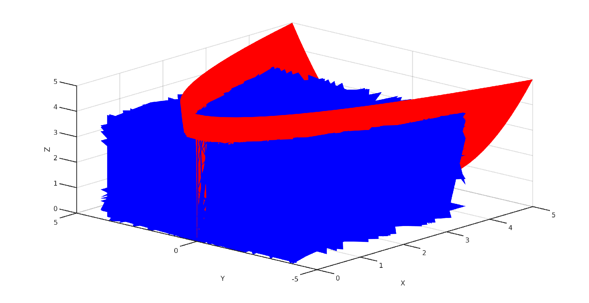
A numerical investigation of (19) reveals that by increasing the number of samples $\mathchar 29037$, the space formed by the intersection of half-spaces (inequality constraints) can fully shrink to the optimal point inside the PSD constraint—see Fig. 1 for an illustrative example of this phenomenon. As can be seen in this figure, the black lines representing the linear inequalities form a finite-volume space around the optimal point displayed by the purple circle inside the PSD cone (the elliptical region²² 2 Note that a two-dimensional slice of the three-dimensional PSD cone typically assumes an elliptical form.) by growing the number of one-bit samples. In (a)/(d), constraints are not enough to create a finite-volume space, whereas in (b)/(e) such constraints can create the desired finite-volume polyhedron space which, however, is not fully inside the PSD cone. Lastly, in (c)/(f), the created finite-volume space shrinks to be fully inside the PSD cone.

To find the signal of interest in the polyhedron (19), we use the RKA without enforcing other costly constraints. This is due to the fact that the solution may be efficiently approached by solving the linear system of inequalities presented in (19).

Note that two signal models for the phase retrieval problem were introduced in [11]: (1) The real-valued model: the unknown signal $\mathbf{\mathchar 29048}$ and $\{\bm{\mathchar 29025}_{\mathchar 29034}\}$ are real. (2) The complex-valued model: the unknown signal $\mathbf{\mathchar 29048}$ and $\{\bm{\mathchar 29025}_{\mathchar 29034}\}$ are complex [11]. Both settings will be considered in the following proposed algorithm.

To recover the desired signal in the one-bit phase retrieval problem, we aim to find a point in the polyhedron (19) instead of solving the SDP in (6). As discussed in Section III-A, when we exploit a large number of samples, the solution of (19) is increasingly likely to capture the desired point, i.e. the signal of interest, inside the PSD conical region. The proposed signal recovery relies on the RKA, which is a powerful tool for solving real- or complex-valued linear system of equations, or inequalities through projections [39, 40].

Accordingly, we propose an algorithm to find the desired matrix $\bm{\mathchar 29016}^{\mathchar 8511}$ in (13) by (i) using abundant measurements, in order to create the finite-volume space inside the PSD conical region (discussed further in Section IV), and (ii) solving (19) via the RKA. We name our algorithm the One-bit Phase Retrieval Algorithm (OPeRA).

The RKA is a sub-conjugate gradient method to solve overdetermined linear systems, i.e, $\bm{\mathchar 28995}\mathbf{\mathchar 29048}\mathchar 12820\mathbf{\mathchar 29026}$ where $\bm{\mathchar 28995}$ is a ${\mathchar 29037\mathchar 8706\mathchar 29038}$ matrix with $\mathchar 29037\mathchar 12606\mathchar 29038$ [40, 41]. Conjugate-gradient methods immediately turn the mentioned inequality to an equality in the following form:

and then, approach the solution by the same process as used for systems of equations. Without loss of generality, consider (20) to be a polyhedron:

where the disjoint index sets $\mathchar 29001_{\mathchar 12820}$ and $\mathchar 29001_{\mathchar 12349}$ partition our sample index set $\mathcal{\mathchar 29002}$, and $\{\bm{\mathchar 29027}_{\mathchar 29034}\}$ denote the rows of $\bm{\mathchar 28995}$. Based on this problem, the projection coefficient $\mathchar 28940_{\mathchar 29033}$ of the RKA is defined as [40, 39, 42]:

Also, the unknown column vector $\mathbf{\mathchar 29048}$ is iteratively updated as:

where, at each iteration $\mathchar 29033$, the index $\mathchar 29034$ is chosen independently at random from the set $\mathcal{\mathchar 29002}$, following the distribution

To ensure a limited error, the feasible region in (19) cannot be an infinite space in an asymptotic sense. Fortunately, by introducing more samples, the problem can form a polyhedron with a bounded volume containing the desired point. Even more interesting, by adding more inequality constraints in (19), the shrinkage of the said polyhedron will put a downward pressure on the error between the desired and recovered points (each informative sample will shrink this space). We will show that by increasing the number of constraints and effective sampling, this error approaches zero. Moreover, as a result of using an overdetermined linear system of inequalities, the convergence of the RKA is guaranteed [40, 39].

It is worth noting that, in our problem, we only have the inequality partition $\mathchar 29001_{\mathchar 12820}$. Herein, the row vectors $\{\bm{\mathchar 29027}_{\mathchar 29034}\}$ and the scalars $\{\mathchar 29026_{\mathchar 29034}\}$ used in the RKA (21)-(24) are $\mathchar 8704\left\{\mathchar 29042_{\mathchar 29034}\operatorname{\delimiter 69640972\mathchar 29029\mathchar 29027}\left\delimiter 67273472\bm{\mathchar 29014}^{\mathchar 574}_{\mathchar 29034}\right\delimiter 84054785^{\mathchar 574}\right\}$ and $\mathchar 8704\left\{\mathchar 29042_{\mathchar 29034}\mathchar 28956^{\mathchar 28722}_{\mathchar 29034}\right\}$, respectively.

We numerically examine the effect of growing the sample size in the recovery of the desired matrix $\bm{\mathchar 29016}^{\mathchar 8511}$ in OPeRA. We will use the spectral radius metric which is particularly informative in the recovery of rank-one matrices. Note that for a positive semi-definite matrix such as our desired matrix $\bm{\mathchar 29016}^{\mathchar 8511}$, the spectral radius is equal to the Frobenius norm of the matrix [38]. In all experiments, the input signals were generated as $\mathbf{\mathchar 29048}\mathchar 12824\mathcal{\mathchar 29006}\left\delimiter 67273472\mathbf{\mathchar 28720}\mathchar 24891\mathchar 29001_{\mathchar 29038}\right\delimiter 84054785\mathchar 8235\mathchar 29034\mathcal{\mathchar 29006}\left\delimiter 67273472\mathbf{\mathchar 28720}\mathchar 24891\mathchar 29001_{\mathchar 29038}\right\delimiter 84054785$ for the complex-valued model, and $\mathbf{\mathchar 29048}\mathchar 12824\mathcal{\mathchar 29006}\left\delimiter 67273472\mathbf{\mathchar 28720}\mathchar 24891\mathchar 29001_{\mathchar 29038}\right\delimiter 84054785$, for the real-valued model. For both models, the rows of the sensing matrix $\bm{\mathchar 28993}$ were generated as $\bm{\mathchar 29025}_{\mathchar 29034}\mathchar 12824\mathcal{\mathchar 29006}\left\delimiter 67273472\mathbf{\mathchar 28720}\mathchar 24891\mathchar 29001_{\mathchar 29038}\right\delimiter 84054785$. Accordingly, we made use of the time-varying thresholds $\bm{\mathchar 28956}\mathchar 12824\operatorname{\mathchar 29004\mathchar 29039\mathchar 29031\mathchar 29038\mathchar 29039\mathchar 29042\mathchar 29037\mathchar 29025\mathchar 29036}\left\delimiter 67273472\mathchar 28720\mathchar 24891\mathchar 28721\right\delimiter 84054785$. We define the experimental mean square error (MSE) between the true spectral radius $\mathchar 28954\left\delimiter 67273472\bm{\mathchar 29016}\right\delimiter 84054785$ and its estimate $\mathchar 28954\left\delimiter 67273472\bar{\bm{\mathchar 29016}}\right\delimiter 84054785$ as

where $\mathchar 28997$ is the number of experiments. Each presented data point is averaged over $\mathchar 28721\mathchar 28720$ experiments. The results are obtained for the number of samples $\mathchar 29037\mathchar 12850\left\{\mathchar 28721\mathchar 28720\mathchar 28720\mathchar 28720\mathchar 24891\mathchar 28725\mathchar 28720\mathchar 28720\mathchar 28720\mathchar 24891\mathchar 28721\mathchar 28720\mathchar 28720\mathchar 28720\mathchar 28720\mathchar 24891\mathchar 28725\mathchar 28720\mathchar 28720\mathchar 28720\mathchar 28720\mathchar 24891\mathchar 28721\mathchar 28720\mathchar 28720\mathchar 28720\mathchar 28720\mathchar 28720\right\}$.

Fig. 2 appears to confirm the possibility of recovering the spectral radius of $\bm{\mathchar 29016}^{\mathchar 8511}$ from the large number of one-bit sampled data with time-varying thresholds by OPeRA for the real-valued and the complex-valued models, respectively. As expected, the performance of the recovery will be significantly enhanced as the number of one-bit samples grows large. In all experiments, the obtained maximum eigenvalue is positive, which is equal to the spectral radius of the recovered matrix.

An important part of our work is to show that our method can recover an $\bm{\mathchar 29016}$ that is “increasingly” rank-one and PSD by growing the number of one-bit sampled data. To do so, at first, we show in Fig. 2 that the maximum eigenvalue is accurately recovered. Next, we present that all eigenvalues $\{\mathchar 352_{\mathchar 29033}\}$ of the recovered matrix $\bar{\bm{\mathchar 29016}}$ except the maximum eigenvalue approach zero by increasing the number of one-bit sampled data. Fig. 3 appears to confirm this claim for both real-valued and complex-valued models. The presented results are averaged over $\mathchar 28721\mathchar 28720$ experiments and the eigenvalues are arranged in descending order.

To further investigate the effectiveness of OPeRA in both real-valued and complex-valued models, Fig. 4 illustrates the squared Frobenius norm of the error normalized by the squared Frobenius norm of the desired matrix $\bm{\mathchar 29016}^{\mathchar 8511}$, defined as

where the presented results are averaged over $\mathchar 28721\mathchar 28720$ experiments. Fig. 4 appears to confirm that the performance of the recovery is enhanced by increasing the number of one-bit samples.

We first investigate the convergence of OPeRA through a probabilistic lens. Define the distance between the optimal point $\bm{\mathchar 29016}^{\mathchar 8511}$ and the $\mathchar 29034$-th hyperplane presented in (19) as

where $\bm{\mathchar 29016}_{\mathchar 29033}$ is the solution from the RKA iterations. From an intuitive point of view, it is easy to observe that by generally reducing the distances between $\bm{\mathchar 29016}^{\mathchar 8511}$ and the constraint-associated hyperplanes, the possibility of capturing the optimal point is increased.

Suppose $\mathcal{\mathchar 29003}$ is the cardinality of the set of the hyperplanes presented in (19), a portion of the whole sample size, i.e., $\mathcal{\mathchar 29003}\mathchar 12820\mathchar 29037$ , which will effectively form a polyhedron inside the PSD cone around the optimal point $\bm{\mathchar 29016}^{\mathchar 8511}$ if the number of samples is sufficient. The average of the distances $\left\{\mathchar 29000_{\mathchar 29034}\right\}$ around the optimal point is obtained as

For a specific sample size $\mathchar 29037$, when the area of the finite-volume space around the optimal point is reduced, $\mathcal{\mathchar 28997}\left\delimiter 67273472\bm{\mathchar 29016}^{\mathchar 8511}\right\delimiter 84054785$ is diminished as well. Define the overall average distance $\mathchar 29012_{\text{ave}}$ as

Increasing the number of samples leads to smaller values of $\mathcal{\mathchar 28997}\left\delimiter 67273472\bm{\mathchar 29016}^{\mathchar 8511}\right\delimiter 84054785$ and $\mathchar 29012_{\text{ave}}$. Therefore, the possibility of creating the finite-volume space around the desired point increases in the asymptotic sample-size scenario, with $\mathchar 29037\mathchar 12821\mathchar 29037^{\mathchar 8511}$, where $\mathchar 29037^{\mathchar 8511}$ is the minimal measurement size. The Chernoff Bound [43, 44] can shed light on this phenomenon as illustrated bellow.

In order to find the signal of interest in the polyhedron (19), we are utilizing the RKA which leads to the following convergence bound [45, 41, 39, 40]:

where $\mathbf{\mathchar 29048}^{\mathchar 8511}$ is a desired point, $\mathchar 29041\mathchar 12850\delimiter 67273472\mathchar 28720\mathchar 24891\mathchar 28721\delimiter 84054785$ is a function of the condition number of the matrix $\bm{\mathchar 28995}$, and $\mathchar 29033$ is the number of required iterations for the RKA. In our problem, $\mathbf{\mathchar 29048}_{\mathchar 29033}\mathchar 12349\operatorname{\delimiter 69640972\mathchar 29029\mathchar 29027}\left\delimiter 67273472\bm{\mathchar 29016}_{\mathchar 29033}\right\delimiter 84054785$, $\mathbf{\mathchar 29048}^{\mathchar 8511}\mathchar 12349\operatorname{\delimiter 69640972\mathchar 29029\mathchar 29027}\left\delimiter 67273472\bm{\mathchar 29016}^{\mathchar 8511}\right\delimiter 84054785$, and $\bm{\mathchar 28995}\mathchar 12349\bm{\mathchar 29010}\mathchar 8716\bm{\mathchar 29014}$. Therefore, the right-hand side of (36) may be recast as

It is clear from (36) that by using a well-chosen initial point $\mathbf{\mathchar 29048}_{\mathchar 28720}$ or by increasing the number of iterations $\mathchar 29033$, the recovery error can be further contained. Nevertheless, in the proposed recovery approach, it is deemed necessary to have the sufficient number of samples (inequalities) in order to guarantee a finite-volume feasible region and a bounded recovery error. Once our search area is located inside the PSD cone, we may effectively employ (36) for the convergence rate. The convergence rate of the RKA is useful when we have a linear system of inequalities. On the other hand, in the one-bit phase retrieval, the main constraints, i.e. the rank-one and the PSD, are non-linear and they may be considered to be redundant by deploying the enough number of samples. Thus, (36) is insufficient to present the convergence rate of OPeRA. We can make (36) relevant to the one-bit phase retrieval problem by taking a penalty function into consideration:

where $\mathchar 28681\delimiter 67273472\mathchar 314\delimiter 84054785$ is a decreasing function in the abundance sample-size regime, such that if the number of samples is enough to satisfy the PSD constraint, the penalty function approaches zero $\mathchar 28681\left\delimiter 67273472\mathchar 29037\right\delimiter 84054785\mathchar 12833\mathchar 28720$. Based on our discussion in Section IV-A, a good example for $\mathchar 28681\left\delimiter 67273472\mathchar 29037\right\delimiter 84054785$ can be $\mathchar 29005_{\mathchar 29012}\mathchar 8704\mathchar 29005_{\mathchar 561}$, where $\mathchar 29005_{\mathchar 561}\mathchar 12349\lim_{\mathchar 29037\mathchar 12833\mathchar 561}\mathchar 29005_{\mathchar 29012}$.

To find a bound for the sufficient number of measurements $\mathchar 29037$ to create a finite-volume space inside the PSD cone and the penalty function starts to be zero, we utilize the tail function of the penalty given by

Tails of decreasing functions may be asymptotically approximated by an exponential function [44]. Mathematically, this may be expressed as

where $\mathchar 28962$ is an arbitrarily small positive number. Therefore, the boundary (38) is reformulated for $\mathchar 29037\mathchar 12821\mathchar 29037^{\mathchar 8511}$ as

The algorithm termination criterion is considered to be

Based on this criterion and (41), the following theorem is presented in order to find a lower bound for the number of required measurements in OPeRA.

The sufficient number of measurements $\mathchar 29037$ is sought to create a finite-volume in the PSD cone $\bm{\mathchar 29016}\mathchar 12823\mathchar 28720$ for the input signal $\mathbf{\mathchar 29048}$ with the size $\mathchar 29038$. It is easy to verify that the dimension of the PSD cone is equal to ${{\mathchar 29038^{\mathchar 28722}\mathchar 8235\mathchar 29038\over\mathchar 28722}}$ in both real-valued and complex valued cases. The infimum number of the hyperplanes creating a finite-volume space in a $\mathchar 29038^{\mathchar 560}$-dimensional region is $\mathchar 29038^{\mathchar 560}\mathchar 8235\mathchar 28721$. Consequently, we can write:

Therefore, to form the finite-volume space, the sample size $\mathchar 29037$ must be lower bounded by $\inf\mathcal{\mathchar 29003}$:

The above bound helps us to establish a clear connection between the sample size and the problem dimension. However, since the boundary in (43) is concerned with containing the error after a finite-volume is formed, it is asymptotically tighter than (48). Therefore, by satisfying (43), the lower bound in (48) is typically met as well.

To compare the computational time for the SDP-based PhaseLift approach and our proposed method, the iterative algorithms are terminated according to (42) with $\mathchar 28943_{\mathchar 28721}\mathchar 12349\mathchar 28721\mathchar 28720^{\mathchar 8704\mathchar 28722}$. The unknown signal $\mathbf{\mathchar 29048}$ lies within $\mathbb{\mathchar 29010}^{\mathchar 28721\mathchar 28720}$. The number of samples $\mathchar 29037$ is set to be $\mathchar 28721\mathchar 28720\mathchar 28720$, $\mathchar 28721\mathchar 28720\mathchar 28720\mathchar 28720$, $\mathchar 28723\mathchar 28720\mathchar 28720\mathchar 28720$, $\mathchar 28724\mathchar 28720\mathchar 28720\mathchar 28720$, $\mathchar 28725\mathchar 28720\mathchar 28720\mathchar 28720$, $\mathchar 28721\mathchar 28720\mathchar 28720\mathchar 28720\mathchar 28720$, $\mathchar 28723\mathchar 28720\mathchar 28720\mathchar 28720\mathchar 28720$, $\mathchar 28725\mathchar 28720\mathchar 28720\mathchar 28720\mathchar 28720$, $\mathchar 28728\mathchar 28720\mathchar 28720\mathchar 28720\mathchar 28720$, and $\mathchar 28721\mathchar 28720\mathchar 28720\mathchar 28720\mathchar 28720\mathchar 28720$. Each CPU time is obtained by averaging over $\mathchar 28725$ experiments. PhaseLift is applied to the high-resolution samples, whereas OPeRA is applied to their one-bit sampled data counterpart, which means only partial information is made available to OPeRA.

As can be seen in Fig. 5, due to the growing number of samples, the cost of the PhaseLift algorithm has an increasing trend. Nevertheless, the CPU time for OPeRA experiences a significant decline rate from $\mathchar 29037\mathchar 12349\mathchar 28721\mathchar 28720\mathchar 28720$ up until $\mathchar 29037\mathchar 12349\mathchar 28725\mathchar 28720\mathchar 28720\mathchar 28720\mathchar 28720$, while it starts increasing afterwards. The reason behind this behavior is hidden in the application of RKA. As discussed in Section IV, to create a finite-volume space around the optimal point $\bm{\mathchar 29016}^{\mathchar 8511}$, and to capture error upper bound $\mathchar 28943_{\mathchar 28721}$, the number of samples has to move to the large-scale regimen. One may simply verify that, according to Theorem 2, by increasing the number of measurements $\mathchar 29037$, the RKA may achieve the error upper bound with fewer iterations $\mathchar 29033$. Additionally, the computational cost of the RKA used to solve (19) behaves as $\mathcal{\mathchar 29007}\left\delimiter 67273472\mathchar 29033\mathchar 29038^{\mathchar 28722}\right\delimiter 84054785$. As a result, the CPU time for OPeRA may initially decrease with a growing number of samples.

Surpassing $\mathchar 29037\mathchar 12349\mathchar 28723\mathchar 28720\mathchar 28720\mathchar 28720$, the CPU time for OPeRA becomes smaller than that of the PhaseLift method; i.e. by employing sufficient number of samples, less complexity is achievable which is facilitated by dropping the PSD constraint. However, after approaching $\mathchar 29037\mathchar 12349\mathchar 28725\mathchar 28720\mathchar 28720\mathchar 28720\mathchar 28720$, we have increased the number of inequalities in such a way that the contribution to signal recovery is negligible, while at the same time, the extra measurements will still need processing. These extra inequalities may require more iterations to take them into account which is undesirable and increases the CPU time; see Fig. 5. Interestingly, OPeRA can satisfy the recovery criterion (42) with less CPU time and less input information compared to PhaseLift which is useful for the high-resolution scenario.

Next, we compare the CPU time of the one-bit PhaseLift defined in (14) and that of OPeRA. As mentioned before, the one-bit PhaseLift problem is a SDP similar to the problem (6).

To compare the relaxation-based formulation of the one-bit PhaseLift with our approach, we aim at the recovery of a signal $\mathbf{\mathchar 29048}\mathchar 12850\mathbb{\mathchar 29010}^{\mathchar 28721\mathchar 28720}$ with sample sizes $\mathchar 29037\mathchar 12850\left\{\mathchar 28721\mathchar 28720\mathchar 28720\mathchar 28720\mathchar 24891\mathchar 28723\mathchar 28720\mathchar 28720\mathchar 28720\mathchar 24891\mathchar 28725\mathchar 28720\mathchar 28720\mathchar 28720\mathchar 24891\mathchar 28728\mathchar 28720\mathchar 28720\mathchar 28720\mathchar 24891\mathchar 28721\mathchar 28720\mathchar 28720\mathchar 28720\mathchar 28720\right\}$. The termination criterion of both algorithms is exactly similar to the one in Section V-A.

As can be seen in Fig. 6, by growing the number of one-bit samples, the CPU time of the one-bit PhaseLift is increasing. On the other hand, the CPU time of OPeRA is decreasing. One may conclude that in the large sample size regimen, the proposed one-bit phase retrieval approach has a lower computational burden than one-bit PhaseLift. This due to enjoying the advantages of using more samples to make both the rank-one constraint and the PSD constraint redundant. We hypothesis that the computation time rise due to unhelpful extra samples (in achieving the error bound) occur well beyond $\mathchar 29037\mathchar 12349\mathchar 28721\mathchar 28720\mathchar 28720\mathchar 28720\mathchar 28720$, which is presumably why the increase is not observed in our experiment.

In light of previous discussion, to achieve a better recovery accuracy for a specific sample size $\mathchar 29037$, one may use the idea of shrinking the space imposed by the set of inequalities in (19) around the optimal solution $\bm{\mathchar 29016}^{\mathchar 8511}$. To make this happen, we propose an iterative algorithm generating an adaptive threshold to accurately obtain the desired solution. To diminish the area of the finite-volume space around the optimal point, we update the time-varying threshold as

where $\left\{\mathchar 28943_{\mathchar 29034}^{\delimiter 67273472\mathchar 29035\delimiter 84054785}\right\}$ at the $\mathchar 29034$-th element of a positive vector $\bm{\mathchar 28943}^{\delimiter 67273472\mathchar 29035\delimiter 84054785}$ in the $\mathchar 29035$-th iteration. This updating process is based on the fact that when $\mathchar 29042_{\mathchar 29034}\mathchar 12349\mathchar 8235\mathchar 28721$, we have $\operatorname{\mathchar 29012\mathchar 29042}\left\delimiter 67273472\bm{\mathchar 29014}_{\mathchar 29034}\bm{\mathchar 29016}\right\delimiter 84054785\mathchar 12821\delimiter 67273472\mathchar 28956_{\mathchar 29034}\delimiter 84054785^{\mathchar 28722}$, and $\operatorname{\mathchar 29012\mathchar 29042}\left\delimiter 67273472\bm{\mathchar 29014}_{\mathchar 29034}\bm{\mathchar 29016}\right\delimiter 84054785\mathchar 12820\delimiter 67273472\mathchar 28956_{\mathchar 29034}\delimiter 84054785^{\mathchar 28722}$ otherwise. The reason behind updating the one-bit measurements $\left\{\mathchar 29042_{\mathchar 29034}^{\delimiter 67273472\mathchar 29035\delimiter 84054785}\right\}$, is to ensure that the optimal solution $\bm{\mathchar 29016}^{\mathchar 8511}$ satisfies (19) in iteration $\mathchar 29035$, i.e. the inequalities $\mathchar 29042_{\mathchar 29034}^{\delimiter 67273472\mathchar 29035\delimiter 84054785}\operatorname{\delimiter 69640972\mathchar 29029\mathchar 29027}\left\delimiter 67273472\bm{\mathchar 29014}^{\mathchar 574}_{\mathchar 29034}\right\delimiter 84054785^{\mathchar 574}\operatorname{\delimiter 69640972\mathchar 29029\mathchar 29027}\left\delimiter 67273472\bm{\mathchar 29016}^{\mathchar 8511}\right\delimiter 84054785\mathchar 12821\mathchar 29042_{\mathchar 29034}^{\delimiter 67273472\mathchar 29035\delimiter 84054785}\left\delimiter 67273472\mathchar 28956_{\mathchar 29034}^{\delimiter 67273472\mathchar 29035\delimiter 84054785}\right\delimiter 84054785^{\mathchar 28722}$ for $\mathchar 29034\mathchar 12850\mathcal{\mathchar 29002}$. Our proposed iterative method to update the time-varying threshold is summarized in Algorithm 1.

To present the efficacy of the adaptive time-varying threshold algorithm in comparison with a non-negative random threshold, the unknown signal $\mathbf{\mathchar 29048}$ and the sensing matrix $\bm{\mathchar 28993}$ are generated using the same settings as in Section III-C. As can be seen in Fig. 8, the performance of our proposed algorithm is evaluated by the NMSE defined in (26) which is considerably enhanced in comparison with adopting a non-negative random threshold according to $\operatorname{\mathchar 29004\mathchar 29039\mathchar 29031\mathchar 29038\mathchar 29039\mathchar 29042\mathchar 29037\mathchar 29025\mathchar 29036}\left\delimiter 67273472\mathchar 28720\mathchar 24891\mathchar 28721\right\delimiter 84054785$. The results are obtained for the sample sizes $\mathchar 29037\mathchar 12850\left\{\mathchar 28721\mathchar 28720\mathchar 28720\mathchar 28720\mathchar 24891\mathchar 28725\mathchar 28720\mathchar 28720\mathchar 28720\mathchar 24891\mathchar 28721\mathchar 28720\mathchar 28720\mathchar 28720\mathchar 28720\mathchar 24891\mathchar 28725\mathchar 28720\mathchar 28720\mathchar 28720\mathchar 28720\mathchar 24891\mathchar 28721\mathchar 28720\mathchar 28720\mathchar 28720\mathchar 28720\mathchar 28720\right\}$ and $\mathchar 28942\mathchar 12349\mathchar 28721\mathchar 28720^{\mathchar 8704\mathchar 28723}$. Each presented data point is averaged over $\mathchar 28725$ experiments.

In the following, we compare the number of measurements $\mathchar 29037$ required to recover the rank-one and PSD matrix $\bm{\mathchar 29016}^{\mathchar 8511}$ using the OPeRA with (i) our proposed adaptive threshold algorithm, as well as (ii) a random non-negative threshold. The result can be summarized as follows.

To numerically scrutinize our claim in Theorem 3, Table I illustrates that the sufficient number of samples $\mathchar 29037$ required for OPeRA to recover a PSD matrix with adaptive sampling thresholds proposed in Algorithm 1 is much less than that of OPeRA with a random threshold. The result is obtained for the input signal $\mathbf{\mathchar 29048}$, a random time-varying threshold $\bm{\mathchar 28956}$, and the sensing matrix $\bm{\mathchar 28993}$ originating from the same settings as presented in Section III-C. The number of samples examined in our experiments are same as Section V-A, plus $\mathchar 29037\mathchar 12349\mathchar 28725\mathchar 28720\mathchar 28720$.

To further investigate the effectiveness of Algorithm 1, we show that the average of all eigenvalues $\{\mathchar 352_{\mathchar 29033}\}$ of $\bar{\bm{\mathchar 29016}}$ except the maximum eigenvalue (spectral radius) approaches zero by increasing the number of measurements—see Fig. 9. Interestingly, Fig. 9 reaffirms that the number of measurements used to recover the rank-one and PSD matrix $\bm{\mathchar 29016}^{\mathchar 8511}$ by OPeRA with adaptive thresholding, is much less than the same result reported in Fig. 3 where OPeRA with a random threshold is adopted. The results are obtained for the number of samples $\mathchar 29037\mathchar 12850\left\{\mathchar 28723\mathchar 28720\mathchar 28720\mathchar 24891\mathchar 28725\mathchar 28720\mathchar 28720\mathchar 24891\mathchar 28721\mathchar 28720\mathchar 28720\mathchar 28720\mathchar 24891\mathchar 28722\mathchar 28720\mathchar 28720\mathchar 28720\right\}$, they are averaged over $\mathchar 28725$ experiments, and the non-dominant eigenvalues are arranged in a decreasing order.

Define the positive-valued vector $\bm{\mathchar 28950}\mathchar 12349\left\delimiter 67482370\mathchar 28950_{\mathchar 28721}\mathchar 24891\mathinner{\mathpunct{\mathchar 513}\mathpunct{\mathchar 513}\mathpunct{\mathchar 513}}\mathchar 24891\mathchar 28950_{\mathchar 29037}\right\delimiter 84267779$ by

Let $\bm{\mathchar 28949}$ and $\mathbf{\mathchar 29050}$ denote the time-varying threshold vector and the noise vector, respectively. The noisy one-bit samples are generated as

The occurrence probability vector $\bm{\mathchar 29040}$ for the noisy one-bit measurement $\bm{\mathchar 29042}$ is given as [46],

where $\mathchar 28680\delimiter 67273472\mathchar 314\delimiter 84054785$ is the CDF of $\mathchar 8704\mathbf{\mathchar 29050}$. Since $\{\mathchar 28950_{\mathchar 29034}\}$ are linear function of $\bm{\mathchar 29016}$, the CDF of noise $\left\{\mathchar 28680\delimiter 67273472\mathchar 28950_{\mathchar 29034}\mathchar 8704\mathchar 28949_{\mathchar 29034}\delimiter 84054785\right\}$ can be written as $\mathchar 28680\left\delimiter 67273472\bm{\mathchar 29016}\right\delimiter 84054785$. The log-likelihood function of the sign data $\bm{\mathchar 29042}$ is given by

Interestingly, by solving the maximum log-likelihood estimation (MLE) problem associated with (53), our desired matrix $\bm{\mathchar 29016}^{\mathchar 8511}$ can be immediately approximated. The proposed algorithm is called Noisy OPeRA.

A preliminary formulation of our optimization problem based on the MLE may be cast as:

This problem is the one-bit version of its counterpart formulated in [23]. However, as discussed in previous sections, because of employing one-bit sampling, the large number of samples can be adopted which leads to the availability of a large number of sign data $\left\{\mathchar 29042_{\mathchar 29034}\right\}$ and the corresponding inequality constraints; since when $\mathchar 29042_{\mathchar 29034}\mathchar 12349\mathchar 8235\mathchar 28721$, we have $\operatorname{\mathchar 29012\mathchar 29042}\left\delimiter 67273472\bm{\mathchar 29014}_{\mathchar 29034}\bm{\mathchar 29016}\right\delimiter 84054785\mathchar 12821\delimiter 67273472\mathchar 28956_{\mathchar 29034}\delimiter 84054785^{\mathchar 28722}$, and $\operatorname{\mathchar 29012\mathchar 29042}\left\delimiter 67273472\bm{\mathchar 29014}_{\mathchar 29034}\bm{\mathchar 29016}\right\delimiter 84054785\mathchar 12820\delimiter 67273472\mathchar 28956_{\mathchar 29034}\delimiter 84054785^{\mathchar 28722}$ otherwise. These inequalities are collected to form the polyhedron (19). However, these constraints may be equivalently absorbed in the objective function to facilitate the one-bit phase retrieval formulation in the noisy case. Therefore, the problem (55) can be reformulated as

In many cases, $\mathcal{\mathchar 29004}_{\bm{\mathchar 29042}}\delimiter 67273472\bm{\mathchar 28950}\mathchar 24891\bm{\mathchar 29016}\delimiter 84054785$ is a concave function and thus the above programs becomes convex. One can readily verify this in the case of a Gaussian noise [35]. In the rest of our paper, $\mathchar 8704\mathbf{\mathchar 29050}$ is assumed to be an i.i.d. zero-mean Gaussian process $\mathbf{\mathchar 29050}\mathchar 12824\mathcal{\mathchar 29006}\left\delimiter 67273472\mathchar 28720\mathchar 24891\mathchar 28955^{\mathchar 28722}_{\mathbf{\mathchar 29050}}\bm{\mathchar 29001}_{\mathchar 29037}\right\delimiter 84054785$, for which $\mathchar 28680\delimiter 67273472\mathchar 314\delimiter 84054785$ is given in (1).

To examine the performance of Noisy OPeRA in practice, and to validate the theoretical results described in this section, we consider signal recovery with different values of $\mathchar 28955_{\mathbf{\mathchar 29050}}\mathchar 12850\left\{\mathchar 28720\mathchar 314\mathchar 28721\mathchar 24891\mathchar 28720\mathchar 314\mathchar 28722\mathchar 24891\mathchar 28720\mathchar 314\mathchar 28724\mathchar 24891\mathchar 28720\mathchar 314\mathchar 28725\mathchar 24891\mathchar 28720\mathchar 314\mathchar 28727\mathchar 24891\mathchar 28721\right\}$, where the unknown signal $\mathbf{\mathchar 29048}$ was generated in a similar manner as in Section III-C. The stochastic threshold $\bm{\mathchar 28949}$ was generated according to $\bm{\mathchar 28949}\mathchar 12824\mathcal{\mathchar 29006}\left\delimiter 67273472\mathchar 28720\mathchar 24891\mathchar 29001_{\mathchar 29037}\right\delimiter 84054785$. The signal to noise ratio (SNR) is evaluated as:

In Fig. 10, the recovery performance is illustrated by using the NMSE defined in (26), with the results averaged over $\mathchar 28721\mathchar 28720$ experiments. We report both SNR and NMSE in dB ($\mathchar 28721\mathchar 28720\log\delimiter 67273472\mathchar 314\delimiter 84054785$). As expected, by increasing the SNR, the performance of our method is improved. Furthermore, the performance of the estimation problem formulation in (55) is enhanced by increasing the number of one-bit samples $\mathchar 29037\mathchar 12850\{\mathchar 28725\mathchar 28720\mathchar 28720\mathchar 28720\mathchar 24891\mathchar 28721\mathchar 28720\mathchar 28720\mathchar 28720\mathchar 28720\}$. In this approach, since the desired matrix $\bm{\mathchar 29016}^{\mathchar 8511}$ is recovered statistically from MLE, we compare $\mathchar 28680\left\delimiter 67273472\bm{\mathchar 29016}\right\delimiter 84054785$ and $\mathchar 28680\delimiter 67273472\bar{\bm{\mathchar 29016}}\delimiter 84054785$ by resorting to a widely used statistical distance, known as the Hellinger distance, which was defined in (2). The vector entry-wise formula of the Hellinger distance is given as

where $\{\bar{\mathchar 28950}_{\mathchar 29034}\}$ is the estimated version of $\{\mathchar 28950_{\mathchar 29034}\}$ obtained from (55). As was previously observed, by increasing the value of SNR, Noisy OPeRA performs better in terms of the NMSE . A similar behavior occurs with the Hellinger distance shown in Fig. 11. The Hellinger distance is obtained is very small for all SNR values in this experiment, However, it is decreasing for an increasing SNR, which appears to confirm the recovery of the desired matrix in statistical (noisy) environments by taking advantage of a large number of samples—thus without considering the rank-one and the PSD constraints.

To show the sustained benefit of sample abundance in the noisy case, we compare Noisy OPeRA with Noisy PhaseLift formulation firstly introduced in [23] as

where $\mathchar 28679_{\bm{\mathchar 28950}}\delimiter 67273472\bm{\mathchar 29016}\delimiter 84054785\mathchar 12349\log\left\delimiter 67273472\mathchar 29030\left\delimiter 67273472\bm{\mathchar 29043}\delimiter 69640972\bm{\mathchar 28950}\right\delimiter 84054785\right\delimiter 84054785$, with the noisy measurement vector $\{\mathchar 29043_{\mathchar 29034}\}$ is sampled from a probability distribution $\mathchar 29030\delimiter 67273472\mathchar 314\delimiter 69640972\bm{\mathchar 28950}\delimiter 84054785$, and $\mathchar 28939$ is a positive scalar. For our numerical examinations, we assume the measurement noise is distributed as $\mathbf{\mathchar 29050}\mathchar 12824\mathcal{\mathchar 29006}\left\delimiter 67273472\mathchar 28720\mathchar 24891\mathchar 28720\mathchar 314\mathchar 28722\mathchar 28725\bm{\mathchar 29001}_{\mathchar 29037}\right\delimiter 84054785$ and the termination criterion is $\left\delimiter 0\bm{\mathchar 29016}_{\mathchar 29033}\mathchar 8704\bm{\mathchar 29016}^{\mathchar 8511}\right\delimiter 0_{\mathrm{\mathchar 28998}}^{\mathchar 28722}\mathchar 12820\mathchar 28725\mathchar 8706\mathchar 28721\mathchar 28720^{\mathchar 8704\mathchar 28723}\left\delimiter 0\bm{\mathchar 29016}^{\mathchar 8511}\right\delimiter 0_{\mathrm{\mathchar 28998}}^{\mathchar 28722}$. Table II shows that by using a large number of samples (and making rank-one and PSD constraints redundant) in the noisy one-bit sampling scenario, Noisy OPeRA can recover the signal with a better CPU time for sample sizes $\mathchar 29037\mathchar 12850\left\{\mathchar 28725\mathchar 28720\mathchar 28720\mathchar 28720\mathchar 24891\mathchar 28721\mathchar 28720\mathchar 28720\mathchar 28720\mathchar 28720\mathchar 24891\mathchar 28722\mathchar 28720\mathchar 28720\mathchar 28720\mathchar 28720\right\}$ compared to the noisy PhaseLift method. This is similar to our discussion in the noiseless scenario; see Section V. Interestingly, by growing the number of samples, the NMSE is enhanced more significantly by Noisy OPeRA than that of the noisy PhaseLift method. The results are averaged over $\mathchar 28725$ experiments. The settings of the input signal, time-varying thresholds and the sensing are also chosen in the same way as in Section III-C.

References

- [1] R. P. Millane, “Phase retrieval in crystallography and optics,” J. Opt. Soc. Am. A, vol. 7, no. 3, pp. 394–411, Mar 1990.
- [2] W. Kim and M. H. Hayes, “The phase retrieval problem in x-ray crystallography,” in Proceedings of the Acoustics, Speech, and Signal Processing, 1991. ICASSP-91., 1991 International Conference, USA, 1991, ICASSP ’91, p. 1765–1768, IEEE Computer Society.
- [3] J. R. Fienup, J. C. Marron, T. J. Schulz, and J. H. Seldin, “Hubble space telescope characterized by using phase-retrieval algorithms,” Appl. Opt., vol. 32, no. 10, pp. 1747–1767, Apr 1993.
- [4] J. E. Krist and C. J. Burrows, “Phase-retrieval analysis of pre- and post-repair hubble space telescope images,” Appl. Opt., vol. 34, no. 22, pp. 4951–4964, Aug 1995.
- [5] A. M. Sarnik, “Phase retrieval: A practical application for the space telescope,” in Inverse Optics II, R.H.T. Bates and A. J. Devaney, Eds. International Society for Optics and Photonics, 1985, vol. 0558, pp. 85 – 94, SPIE.
- [6] R. W. Gerchberg and W. O. Saxton, “Phase determination for image and diffraction plane pictures in the electron microscope,” Optik, vol. 34, pp. 275–284, 1971.
- [7] R. W. Gerchberg and W. O. Saxton, “A practical algorithm for the determination of phase from image and diffraction plane pictures,” Optik, vol. 35, pp. 227–246, 1972.
- [8] J. R. Fienup, “Comments on ”the reconstruction of a multidimensional sequence from the phase or magnitude of its Fourier transform”,” IEEE Transactions on Acoustics, Speech, and Signal Processing, vol. 31, no. 3, pp. 738–739, Jun 1983.
- [9] J. R. Fienup, “Phase retrieval algorithms: a comparison,” Appl. Opt., vol. 21, no. 15, pp. 2758–2769, Aug 1982.
- [10] J. R. Fienup, “Reconstruction of an object from the modulus of its Fourier transform,” Opt. Lett., vol. 3, no. 1, pp. 27–29, Jul 1978.
- [11] E. J. Candes, T. Strohmer, and V. Voroninski, “PhaseLift: Exact and stable signal recovery from magnitude measurements via convex programming,” Communications on Pure and Applied Mathematics, vol. 66, no. 8, pp. 1241–1274, 2013.
- [12] E.J. Candès and X. Li, “Solving quadratic equations via PhaseLift when there are about as many equations as unknowns,” Foundations of Computational Mathematics, vol. 14, no. 5, pp. 1017–1026, 2014.
- [13] K. Jaganathan, S. Oymak, and B. Hassibi, “Sparse phase retrieval: Convex algorithms and limitations,” in 2013 IEEE International Symposium on Information Theory. IEEE, 2013, pp. 1022–1026.
- [14] E. J. Candès, X. Li, and M. Soltanolkotabi, “Phase retrieval via Wirtinger flow: Theory and algorithms,” IEEE Transactions on Information Theory, vol. 61, no. 4, pp. 1985–2007, Apr 2015.
- [15] Y. Chen and E. J. Candes, “Solving random quadratic systems of equations is nearly as easy as solving linear systems,” in Advances in Neural Information Processing Systems 28, pp. 739–747. Curran Associates, Inc., 2015.
- [16] R. Kolte and A. Özgür, “Phase retrieval via incremental truncated wirtinger flow,” ArXiv, vol. abs/1606.03196, 2016.
- [17] H. Zhang, Y. Liang, and Y. Chi, “A nonconvex approach for phase retrieval: Reshaped Wirtinger flow and incremental algorithms,” Journal of Machine Learning Research, vol. 18, no. 141, pp. 1–35, 2017.
- [18] S. Nayer and N. Vaswani, “Sample-efficient low rank phase retrieval,” IEEE Transactions on Information Theory, vol. 67, no. 12, pp. 8190–8206, 2021.
- [19] F. Fogel, I. Waldspurger, and A. d’Aspremont, “Phase retrieval for imaging problems,” Mathematical programming computation, vol. 8, no. 3, pp. 311–335, 2016.
- [20] G. Jagatap and C. Hegde, “Fast, sample-efficient algorithms for structured phase retrieval,” Advances in Neural Information Processing Systems, vol. 30, 2017.
- [21] S. Bahmani and J. Romberg, “Phase retrieval meets statistical learning theory: A flexible convex relaxation,” in Artificial Intelligence and Statistics. PMLR, 2017, pp. 252–260.
- [22] H. Sahinoglou and S. D. Cabrera, “On phase retrieval of finite-length sequences using the initial time sample,” IEEE Transactions on Circuits and Systems, vol. 38, no. 8, pp. 954–958, 1991.
- [23] E. J. Candes, Y. C. Eldar, T. Strohmer, and V. Voroninski, “Phase retrieval via matrix completion,” SIAM review, vol. 57, no. 2, pp. 225–251, 2015.
- [24] A. Eamaz, F. Yeganegi, and M. Soltanalian, “Modified arcsine law for one-bit sampled stationary signals with time-varying thresholds,” in ICASSP 2021-2021 IEEE International Conference on Acoustics, Speech and Signal Processing (ICASSP). IEEE, 2021, pp. 5459–5463.
- [25] Texas Instruments, “Analog embedded processing,” Active Filter Design Techniques, Literature Number SLOA088 Texas Instruments, excerpted from OP-Amps for Everyone, Literature Number SLOD006A.
- [26] A. Mezghani and A. L. Swindlehurst, “Blind estimation of sparse broadband massive MIMO channels with ideal and one-bit ADCs,” IEEE Transactions on Signal Processing, vol. 66, no. 11, pp. 2972–2983, 2018.
- [27] S. Sedighi, B. Shankar, M. Soltanalian, and B. Ottersten, “One-bit DoA estimation via sparse linear arrays,” in IEEE International Conference on Acoustics, Speech and Signal Processing (ICASSP). IEEE, 2020, pp. 9135–9139.
- [28] A. Eamaz, F. Yeganegi, and M. Soltanalian, “Covariance recovery for one-bit sampled data with time-varying sampling thresholds—Part I: Stationary signals,” TechRxiv, 2022.
- [29] A. Eamaz, F. Yeganegi, and M. Soltanalian, “Covariance recovery for one-bit sampled data with time-varying sampling thresholds—Part II: Non-stationary signals,” TechRxiv, 2022.
- [30] C. Qian and J. Li, “ADMM for harmonic retrieval from one-bit sampling with time-varying thresholds,” in 2017 IEEE International Conference on Acoustics, Speech and Signal Processing (ICASSP). IEEE, 2017, pp. 3699–3703.
- [31] C. Gianelli, Luzhou Xu, Jian Li, and Petre Stoica, “One-bit compressive sampling with time-varying thresholds for sparse parameter estimation,” in 2016 IEEE Sensor Array and Multichannel Signal Processing Workshop (SAM). IEEE, 2016, pp. 1–5.
- [32] P. Wang, J. Li, M. Pajovic, P. T. Boufounos, and Philip V Orlik, “On angular-domain channel estimation for one-bit massive MIMO systems with fixed and time-varying thresholds,” in 51st Asilomar Conference on Signals, Systems, and Computers. IEEE, 2017, pp. 1056–1060.
- [33] F. Xi, Y. Xiang, S. Chen, and A. Nehorai, “Gridless parameter estimation for one-bit MIMO radar with time-varying thresholds,” IEEE Transactions on Signal Processing, vol. 68, pp. 1048–1063, 2020.
- [34] J. M. Ortega, Numerical analysis: a second course, SIAM, 1990.
- [35] M. A. Davenport, Y. Plan, E. Van Den Berg, and M. Wootters, “1-bit matrix completion,” Information and Inference: A Journal of the IMA, vol. 3, no. 3, pp. 189–223, 2014.
- [36] L. Vandenberghe and S. Boyd, “Semidefinite programming,” SIAM review, vol. 38, no. 1, pp. 49–95, 1996.
- [37] Y. Nesterov, Introductory lectures on convex optimization: A basic course, vol. 87, Springer Science & Business Media, 2003.
- [38] C. F. Van Loan and G. Golub, “Matrix computations (Johns Hopkins studies in mathematical sciences),” 1996.
- [39] J. Briskman and D. Needell, “Block Kaczmarz method with inequalities,” Journal of Mathematical Imaging and Vision, vol. 52, no. 3, pp. 385–396, 2015.
- [40] D. Leventhal and A. S. Lewis, “Randomized methods for linear constraints: convergence rates and conditioning,” Mathematics of Operations Research, vol. 35, no. 3, pp. 641–654, 2010.
- [41] T. Strohmer and R. Vershynin, “A randomized Kaczmarz algorithm with exponential convergence,” Journal of Fourier Analysis and Applications, vol. 15, no. 2, pp. 262–278, 2009.
- [42] L. Dai, M. Soltanalian, and K. Pelckmans, “On the randomized Kaczmarz algorithm,” IEEE Signal Processing Letters, vol. 21, no. 3, pp. 330–333, 2013.
- [43] H. Chernoff, “A measure of asymptotic efficiency for tests of a hypothesis based on the sum of observations,” The Annals of Mathematical Statistics, pp. 493–507, 1952.
- [44] H. Chernoff, “A career in statistics,” Past, Present, and Future of Statistical Science, vol. 29, 2014.
- [45] Boris T Polyak, “Gradient methods for solving equations and inequalities,” USSR Computational Mathematics and Mathematical Physics, vol. 4, no. 6, pp. 17–32, 1964.
- [46] S. A. Bhaskar and A. Javanmard, “1-bit matrix completion under exact low-rank constraint,” in 2015 49th Annual Conference on Information Sciences and Systems (CISS). IEEE, 2015, pp. 1–6.