PMAL: Open Set Recognition via Robust Prototype Mining

Following Monte-Carlo simulation(Gal and Ghahramani 2016), we first acquire $U$ SoftMax-based deep classifiers $\{M^{u}\}_{u=1}^{U}$ on the training set of known classes by repeating the training process $U$ times. Then the input data is fed into the pre-trained classifiers, obtaining $\{Z^{u}\}_{u=1}^{U}$. Noticing that it is sufficient to formalize different embedding space by conducting repeated training processes with random parameter initialization and data shuffling, as proved in (Lakshminarayanan, Pritzel, and Blundell 2017). Here we set $U$ to 2 for clearer illustration.

Based on Sec. 3.2, the higher quality for a sample, the lower data uncertainty it has.

Property 1. Given a high-quality sample $x_{i}$, its embedding $z_{i}$ satisfies $z_{i}$$\approx$$\phi_{i}$.

The high-quality sample $x_{i}$ satisfy $\sigma_{i}$$\approx$$0$, then combined with Equa. 2 we can easily obtain the above property. Suppose we select high-quality samples from training data to form the candidate prototype set $C$=$\{c_{i}\}_{i=1}^{H}$$\subseteq$$X$, where $H$ is the total candidate number. Correspondingly, the set of their embedding in two different space $Z^{1}$ and $Z^{2}$ can be denoted as $\Phi^{1}$=$\{z_{i}^{1}\}_{i=1}^{H}$$\approx$$\{\phi_{i}^{1}\}_{i=1}^{H}$ and $\Phi^{2}$=$\{z_{i}^{2}\}_{i=1}^{H}$$\approx$$\{\phi_{i}^{2}\}_{i=1}^{H}$, where the superscript denotes the index of embedding space.

Property 2. Given a sample pair $(x_{i},x_{j})$, $\forall$ $i,j$ $\in$$\{1,...H\}$, Mahalanobis distance in embedding space $Z$ can be computed by $d_{\mathcal{M}}(z_{i},z_{j})\text{=}\sqrt{(z_{i}\text{-}z_{j})\varSigma^{-1}(z_{i}\text{-}z_{j})^{\mathrm{T}}}$ where $\varSigma^{-1}$ is covariance matrix. If $x_{i}$, $x_{j}$ are both of high quality, $d_{\mathcal{M}}(z_{i},z_{j})$ in different embedding space remains similar, i.e., $d_{\mathcal{M}}(z_{i}^{1},z_{j}^{1})$$\approx$$d_{\mathcal{M}}(z_{i}^{2},z_{j}^{2})$, $\forall x_{i},x_{j}\in C$.

Proofs. When only feeding the class-relevant feature $\phi_{i}^{1}$ and $\phi_{i}^{2}$ into the top linear layer of each classifier, the output probability for each category should remain consistent under the constraint of same class label $y_{i}$, i.e., $p(\hat{y}_{i}^{1}\text{=}k|\phi_{i}^{1})$$\approx$$p(\hat{y}_{i}^{2}\text{=}k|\phi_{i}^{2})$, $\forall$$k$$\in$$\{1,...,K\}$. Combining Equa. 1, we have the formulation:

which can be deduced to

Averaging up all the equations for $\forall$ $k$$\in$$\{1,...,K\}$ leads to

where $\overline{w}$=($\sum_{l=1}^{K}{w_{l}}$)/$K$ and $\overline{b}$=($\sum_{l=1}^{K}{b_{l}}$)/$K$. Taking $A$= $(w_{1}-\overline{w},...,w_{K}-\overline{w})$ and $B$=$(b_{1}-\overline{b},...,b_{K}-\overline{b})$, Equa. 5 can be rewritten as $\phi_{i}^{1}A^{1}$+$B^{1}\approx\phi_{i}^{2}A^{2}$+$B^{2}$. Given another $c_{j}$$\in$$C$ where $j$$\neq$$i$, the same equation $\phi_{j}^{1}A^{1}$+$B^{1}\approx\phi_{j}^{2}A^{2}$+$B^{2}$ can be obtained. Combining these two equations leads to $(\phi_{i}^{1}-\phi_{j}^{1})A^{1}\approx(\phi_{i}^{2}-\phi_{j}^{2})A^{2}$, which is equivalent to:

Here, $AA^{\mathrm{T}}\text{=}(w_{1}-\overline{w},...,w_{K}-\overline{w})(w_{1}-\overline{w},...,w_{K}-\overline{w})^{\mathrm{T}}$. As (Chang et al. 2020) pointed out, $w_{n}$$\in$$\{w_{1},...w_{K}\}$ in $A$ can be seen as the center (or mean) of embedding region $Z_{n}$, i.e., $E(z_{i}|y_{i}\text{=}n)$$\approx$$w_{n}$. Thus $AA^{\mathrm{T}}$ is a reasonable estimation for the covariance matrix $\varSigma$^-1 of $Z$. Consequently, Equa. 6 educes $d_{\mathcal{M}}(z_{i}^{1},z_{j}^{1})$$\approx$$d_{\mathcal{M}}(\phi_{i}^{1},\phi_{j}^{1})$$\approx$$d_{\mathcal{M}}(\phi_{i}^{2},\phi_{j}^{2})$$\approx$$d_{\mathcal{M}}(z_{i}^{2},z_{j}^{2})$.

Definition 1. Embedding Topology Robustness. Given a sample $x_{i}$, its relative position to other samples in embedding space $Z$ is defined by ‘embedding topology’ as: $t({z_{i}})\triangleq(d_{\mathcal{M}}(z_{i},z_{1}),...,d_{\mathcal{M}}(z_{i},z_{{N}}))$. Then the distance metric ‘embedding topology robustness’ is defined by:

where $||$$\cdot$$||_{2}$ is Euclidean distance. Following Property 2, $r(\cdot)$ possesses the following characteristic.

Property 3. High-quality samples have large embedding topology robustness $r(\cdot)$ near 1, while low-quality ones correspond to smaller $r(\cdot)$.

For a high-quality sample $x_{i}$$\in$$C$ with data uncertainty $\sigma_{i}$$\approx$0, since $d_{\mathcal{M}}(z_{i}^{1},z_{j}^{1})$$\approx$$d_{\mathcal{M}}(z_{i}^{2},z_{j}^{2})$, $\forall x_{j}$$\in$$C$, then $||t({z_{i}^{1}})-t({z_{i}^{2}})||_{2}$ will be a small value approaching 0, hence robustness $r(x_{i})$ will be a large value near 1.

For a low-quality sample $x_{i}$$\in$($X$$\setminus$$C$) with large uncertainty $\sigma_{i}$, the consistency of Embedding Topology will be disrupted. See Figure 3(a), the Mahalanobis distance from class-relevant feature $\phi_{i}$ to $\phi_{1}$, $\phi_{2}$, $\phi_{3}$ remains similar in $Z^{1}$ and $Z^{2}$ following above analysis, thus the topology shape among $\phi_{(\cdot)}$ (dashed arrows) keeps unchanged. But $z_{{i}}^{1}$ and $z_{{i}}^{2}$ vary evidently caused by $\sigma_{{i}}$, hence topology shape from $z_{i}$ to $\phi_{1}$, $\phi_{2}$, $\phi_{3}$ (green solid arrows) shows great distinctions in two space, which results in a reduced $r(x_{i})$. Obviously, the larger uncertainty $\sigma_{i}$ will trigger larger variation of topology shape, leading to smaller $r(x_{i})$.

We denote the set of all input $x_{i}$ in class $k$ as $\mathrm{S}_{k}$. To generate candidate prototype set $C_{k}$ for class $k$, we first find the sample with the highest embedding topology robustness score, i.e., $\max\{r(x_{i})|x_{i}\in\mathrm{S}_{k}\}$. Then samples with $r(\cdot)$ value above $\epsilon\cdot\max\{r(x_{i})|x_{i}\in\mathrm{S}_{k}\}$ are elected into $C_{k}$, where $\epsilon$ is a preset threshold.

Two backbones are adopted to implement our method. The light-weighted backbone OSCRI (Neal et al. 2018) with parameters less than $1M$ is used to validate our performance when equipped on applications with limited resources. The larger-scale backbone Wide-ResNet (WRN) (Chen et al. 2020) with $9M$ parameters is implemented for a fair comparison with previous methods, whose parameter is still less than most existed methods (Yoshihashi et al. 2019; Oza and Patel 2019; Sun et al. 2020). We adopt Adam optimizer to train our model on each dataset for 600 epochs with batchsize 128. The learning rate starts at 0.01 and is dropped by 0.1 every 120 epochs, momentum is set to 0.9 and weight decay is 5e-4. The same optimization strategy is used for obtaining pre-trained models and for embedding space optimization. For all datasets, the margin $\delta$ is fixed to 0.5, $\lambda_{p}$ is set to 1 and prototype number $T$=10.

Following (Neal et al. 2018), the evaluation includes 2 parts: (1) close set performance of known classes is reported by classification accuracy ACC on test set of knowns, and (2) unknown detection performance is evaluated by the most adopted metric AUROC (Area Under ROC Curve) (Neal et al. 2018) on the test set of both known and unknown classes. Reported results are averaged over 5 random splits. We observe two rejection rules lead to similar results, thus we simply report the results of DR.

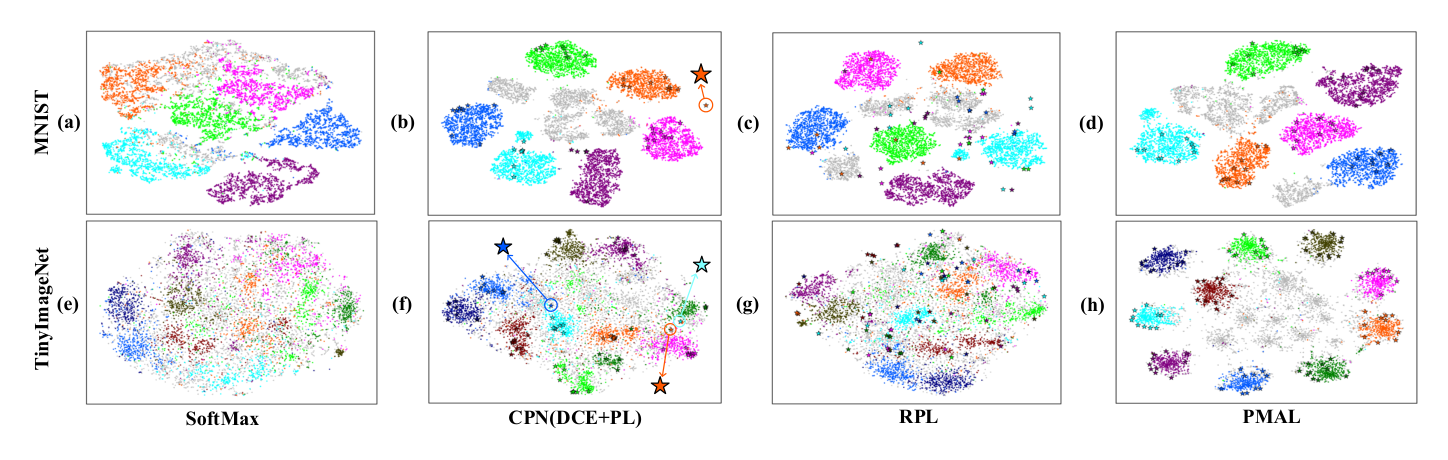
(1) Close Set Recognition: Table 1 shows we obtain the best ACC on all datasets, especially the gain reaches 2%$\sim$3% on three CIFAR datasets and TINY. We attribute it to the fact that PMAL learns more compact intra-class embedding compared to other methods (shown in Figure 6(e)$\sim$(h), thus the classification decision boundaries among classes can be more correctly drawn. (2) Open Set Recognition: PMAL achieves the best AUROC on all benchmarks in Table 1, especially on the most complex TINY, PMAL-WRN achieves 2.2% gain compared to previous best RPL-WRN. The superiority of PMAL is more obvious when equipped on light-weight ‘OSCRI’. Compared to RPL-OSCRI, ARPL and CPN with the same backbone, PMAL-OSCRI outperforms them by a larger margin over 3.6%. Besides, the light PMAL-OSCRI only falls slightly behind PMAL-WRN, still holding top performance among all the reported results (even those with larger networks).

We further validate our method on more challenging large-scale datasets including (1) ImageNet-100, ImageNet-200 (Yang et al. 2020): the first 100 and 200 classes from ImageNet (Deng et al. 2009) are selected as known classes and the rest are treated as unknowns; (2) ImageNet-LT (Liu et al. 2019): a long-tailed dataset with 1000 known classes from ImageNet-2012 (Deng et al. 2009), and additional classes in ImageNet-2010 are as unknowns. The image number per class ranges from 5 to 1280, thus it can well simulate the problem of long-tailed data distribution.

Similar to (Chen et al. 2020), ResNet-50 (He et al. 2016) is used as network backbone and SGD optimizer is adopted with learning rate 0.2, which drops by 0.1 every 30 epochs. Other detailed setups are the same with experiments on small-scale datasets in Section 6.1.

The same metrics (ACC and AUROC) are used for evaluation. See Table 2, our method improves close set ACC by 3.2% and 2% on ImageNet-LT and ImageNet-200. Moreover, open set AUROC is significantly enhanced by 16.5%, 12.6% and 13.7% compared to state-of-the-art. Such performance gains are much more evident than the improvements on small-scale datasets, reflecting that our method possesses larger advantage in more challenging large-scale tasks. It can be observed that the parameter number (apart from the adopted same backbone) of previous methods increases along with known class number, which exceeds a non-negligible cost 2M on ImageNet-LT. The increased prototype parameters may aggravate the difficulty of model training, thus deteriorate their performance. Instead, since PMAL brings no parameters for prototypes, its performance is invariant to the number of known classes, which explains the promotion on more complicated datasets.

Besides, the huge promotion on long-tailed dataset shows PMAL can better handle the problem than the existing. Previous ones tend to learn unreliable prototypes for those few-sample classes, due to unbalanced training of various classes. While PMAL directly mines prototypes from training data, thus produces stable prototypes with fewer samples.

As shown in Table 3, we perform each experiment of the proposed components for ablation study, including the components regarding the two properties, i.e., high-quality and diversity (see Sec. 4), and the embedding learning procedure using the point-to-set distance metric (see Sec. 5.1).

• •

  In prototype mining (PM) phase, both high-quality and diversity matters in prototypes, where high-quality is the more crucial factor validated by our experiments. Jointly combining the two further boosts the performance.

• •

  In embedding optimization (EO) phase, no ‘$\checkmark$’ denotes the commonly adopted way: computing the distance from sample $x_{i}$ to its nearest prototype. Obviously, our proposed point-to-set metric has 1.2% gain, comparing (a)/(c),(b)/(d) or (e)/(f).

(1) Distribution of $r(\cdot)$: We further analyze the distribution of $r(\cdot)$ on TinyImageNet in Figure 4(a). It shows different samples correspond to various robustness, which decreases along with quality degradation caused by occlusion or background interference etc. Besides, we summarize classification accuracy in each interval of $r(\cdot)$, which shows a monotonously ascending trend. It means high-quality samples have larger probabilities to be correctly identified. (2) Comparison with other methods: Furthermore, we compare with mainstream methods to prove the advantage of embedding topology robustness $r(\cdot)$ for selecting high-quality samples on TinyImageNet: (a) Probability: samples with the highest predicted probability from each class are chosen as prototypes; (b) Deep Ensembles (Lakshminarayanan, Pritzel, and Blundell 2017): samples with the lowest probability variance between two models are used as prototypes; (c) MC-dropout (Gal and Ghahramani 2016): data uncertainty is modeled by MC-dropout with ratio 0.5 and samples with the lowest probability variance are selected as prototypes. For a fair comparison, we fix $\epsilon$ to 0.7 and replace $r(\cdot)$ with above ‘probability’ or ‘probability variance’, and then adopt the same diversity strategy to produce final prototypes. Table 5 verifies proposed embedding topology robustness is better than other widely-used data uncertainty modeling methods.

(1) Number of prototypes: We vary prototype number $T$ to quantify the effect of diversity on TinyImageNet. As in Table 5, diverse prototypes lead to much better performance than a single prototype, we obtain the best result when $T$=10. When $T$ increases over 10, performance gradually stabilized. To interpret the advantage of diversity, we visualize embedding space when $T$=1 or $T$=10 in Figure 5(a). Evidently, the chosen 10 prototypes appear in diverse visual looking and their embeddings are located at separate positions. Moreover, using 10 prototypes learns more compact intra-class embedding regions, where unknown sample points are farther from the embedding region of known classes. The reason can be illustrated by Figure 5(b): when $T$=1, sample $s_{B}$ from class B looks even more like the prototype $p_{A}$ of class A than the prototype $p_{B,1}$ of class B, but its embedding will still be forced to be closer to $p_{B,1}$ than $p_{A}$, which is hard to be optimized. Instead when $T$$>$1, embedding of $s_{B}$ is mainly pulled closer to $p_{B,2}$ and $p_{B,3}$ with similar appearance and adjacent embedding, which eases training difficulty. Hence it learns more compact intra-class embedding. (2) Comparison with other methods: We compare with 2 strategies to select multiple ($T$=10) prototypes from same candidates: (a) Randomization: prototypes are randomly selected from candidates. (b) Clustering: K-Means clustering is used and samples whose embedding nearest to cluster centers are used as prototypes. Table 5 shows the obvious advantage using our diversity-based method above randomization and clustering.

The selected prototypes are affected by pre-trained embedding model $M^{1}$ and $M^{2}$. We repeat the mining process for 3 times using different embedding models, and give the results of a class from TinyImageNet in Figure 4(b). We observe prototypes chosen in different repetitions only fluctuate very slightly in embedding space, which validates the stability of prototype mining.

We compare learned embedding space of PL methods in Figure 6. On the easier MNIST dataset, compared to the naive ‘SoftMax’, the latter three can enlarge the distance among known classes.But on the more complex TinyImageNet, our method pushes away the embedding region of known classes to a much larger extent compared to CPN and RPL, so the overlap between known and unknowns is much more evidently reduced.

For CPN, we observe undesired prototypes in the circle of Figure 6(f), arising from the unstable prototype learning fooled by low-quality samples. For RPL, known and unknown samples also can not be well separated by referring to learned prototypes in Figure 6(g). This reveals existed methods endanger from learning sub-optimal prototypes or embedding space especially in complicated tasks. Instead, PMAL is capable of mining trustworthy prototypes and optimizing satisfying embeddings in more challenging tasks.

(1) Threshold $\epsilon$. $\epsilon$ controls the balance of prototype quality and diversity. A larger $\epsilon$ implies more strict condition to ensure quality, but less samples will be elected as candidates, thus diversity among candidates is reduced. A smaller $\epsilon$ is on the contrary. As in Table 5, setting $\epsilon$ too small or large both results in AUROC declined. We find $\epsilon$ in the range [0.6, 0.8] leads to stable performance. (2) Initial model number $U$. Optionally we can adopt more than 2 models to compute $r(\cdot)$, that is, we first compute $r(\cdot)$ with Equation 7 between two arbitrary models then average the results. AUROC remains similar as we increase $U$, shown in Table 5, which implies 2 models are already sufficient to extract effective prototypes. Note that we adopt 2 models for prototype mining, but only one model is employed for prototype learning, thus no extra model parameters are added during inference. (3) Margin $\delta$ and $\lambda_{p}$. $\delta$ decides the separability of different embedding regions. When $\delta$ is too small, different regions can not be well separated. But if $\delta$ becomes too large, $\mathcal{L}_{p}$ will grow to a large value overwhelming $\mathcal{L}_{cls}$, causing $\mathcal{L}_{cls}$ hard to converge. See Table 5, a value between 0.3 and 0.5 for $\delta$ can produce better AUROC results. For loss weight $\lambda_{p}$, when we vary it among 0.5, 0.8 and 1, the resulted AUROC are 82.6, 82.8 and 82.9, which implies PMAL is not very sensitive to $\lambda_{p}$. For all the validations in various tasks, we adopt the universal hyper-parameter setting: $T$=10, $\epsilon$=0.7, $U$=2, $\delta$=0.5 and $\lambda_{p}$=1.

References

- Bendale and Boult (2016) Bendale, A.; and Boult, T. E. 2016. Towards Open Set Deep Networks. In CVPR, 1563–1572.
- Chang et al. (2020) Chang, J.; Lan, Z.; Cheng, C.; and Wei, Y. 2020. Data Uncertainty Learning in Face Recognition. In CVPR, 5709–5718.
- Chen et al. (2021) Chen, G.; Peng, P.; Wang, X.; and Tian, Y. 2021. Adversarial Reciprocal Points Learning for Open Set Recognition. IEEE TPAMI, 1–1.
- Chen et al. (2020) Chen, G.; Qiao, L.; Shi, Y.; Peng, P.; Li, J.; Huang, T.; Pu, S.; and Tian, Y. 2020. Learning Open Set Network with Discriminative Reciprocal Points. In ECCV, volume 12348, 507–522.
- Deng et al. (2009) Deng, J.; Dong, W.; Socher, R.; Li, L.; Li, K.; and Li, F. 2009. ImageNet: A large-scale hierarchical image database. In CVPR, 248–255.
- Gal and Ghahramani (2016) Gal, Y.; and Ghahramani, Z. 2016. Dropout as a Bayesian Approximation: Representing Model Uncertainty in Deep Learning. In ICML, volume 48, 1050–1059.
- Ge, Demyanov, and Garnavi (2017) Ge, Z.; Demyanov, S.; and Garnavi, R. 2017. Generative OpenMax for Multi-Class Open Set Classification. arXiv:1707.07418.
- He et al. (2016) He, K.; Zhang, X.; Ren, S.; and Sun, J. 2016. Deep Residual Learning for Image Recognition. In CVPR, 770–778.
- Kendall, Badrinarayanan, and Cipolla (2016) Kendall, A.; Badrinarayanan, V.; and Cipolla, R. 2016. Bayesian segnet: Model uncertainty in deep convolutional encoder-decoder architectures for scene understanding. arXiv:1511.02680.
- Krizhevsky and et al (2009) Krizhevsky, A.; and et al, G. H. 2009. Learning multiple layers of features from tiny images. Technical report.
- Lakshminarayanan, Pritzel, and Blundell (2017) Lakshminarayanan, B.; Pritzel, A.; and Blundell, C. 2017. Simple and Scalable Predictive Uncertainty Estimation using Deep Ensembles. In NeurIPS, 6402–6413.
- LeCun et al. (1998) LeCun, Y.; Bottou, L.; Bengio, Y.; and Haffner, P. e. a. 1998. Gradient-based learning applied to document recognition. Proceedings of the IEEE, 86(11): 2278–2324.
- Liu et al. (2019) Liu, Z.; Miao, Z.; Zhan, X.; Wang, J.; Gong, B.; and Yu, S. X. 2019. Large-Scale Long-Tailed Recognition in an Open World. In CVPR, 2537–2546.
- Ma et al. (2013) Ma, M.; Shao, M.; Zhao, X.; and Fu, Y. 2013. Prototype based feature learning for face image set classification. In FG, 1–6.
- Neal et al. (2018) Neal, L.; Olson, M. L.; Fern, X. Z.; Wong, W.; and Li, F. 2018. Open Set Learning with Counterfactual Images. In ECCV, volume 11210, 620–635.
- Netzer et al. (2011) Netzer, Y.; Wang, T.; Coates, A.; Bissacco, A.; Wu, B.; and Ng, A. 2011. Reading digits in natural images with unsupervised feature learning. In NeurIPS workshop.
- Oza and Patel (2019) Oza, P.; and Patel, V. M. 2019. C2AE: Class Conditioned Auto-Encoder for Open-Set Recognition. In CVPR, 2307–2316.
- Rosch (1973) Rosch, E. 1973. Natural categories. Cognitive psychology, 4(3): 328–350.
- Scheirer et al. (2013) Scheirer, W. J.; de Rezende Rocha, A.; Sapkota, A.; and Boult, T. E. 2013. Toward Open Set Recognition. IEEE TPAMI, 35(7): 1757–1772.
- Sener and Savarese (2018) Sener, O.; and Savarese, S. 2018. Active Learning for Convolutional Neural Networks: A Core-Set Approach. arXiv:1708.00489.
- Shi and Jain (2019) Shi, Y.; and Jain, A. K. 2019. Probabilistic Face Embeddings. In ICCV, 6901–6910.
- Snell, Swersky, and Zemel (2017) Snell, J.; Swersky, K.; and Zemel, R. S. 2017. Prototypical Networks for Few-shot Learning. In NeurIPS, 4077–4087.
- Sun et al. (2020) Sun, X.; Yang, Z.; Zhang, C.; Ling, K. V.; and Peng, G. 2020. Conditional Gaussian Distribution Learning for Open Set Recognition. In CVPR, 13477–13486.
- Vaswani et al. (2017) Vaswani, A.; Shazeer, N.; Parmar, N.; Uszkoreit, J.; Jones, L.; Gomez, A. N.; Kaiser, L.; and Polosukhin, I. 2017. Attention Is All You Need. In NeurIPS, 6000–6010.
- Wang et al. (2016) Wang, W.; Wang, R.; Shan, S.; and Chen, X. 2016. Prototype Discriminative Learning for Face Image Set Classification. In ACCV, volume 10113, 344–360.
- Ya and Xuan (2015) Ya, L.; and Xuan, Y. 2015. Tiny imagenet visual recognition challenge. CS 231N, 7(7): 3.
- Yang et al. (2018) Yang, H.; Zhang, X.; Yin, F.; and Liu, C. 2018. Robust Classification With Convolutional Prototype Learning. In CVPR, 3474–3482.
- Yang et al. (2020) Yang, H.-M.; Zhang, X.-Y.; Yin, F.; Yang, Q.; and Liu, C.-L. 2020. Convolutional Prototype Network for Open Set Recognition. IEEE TPAMI, 1–1.
- Yoshihashi et al. (2019) Yoshihashi, R.; Shao, W.; Kawakami, R.; You, S.; Iida, M.; and Naemura, T. 2019. Classification-Reconstruction Learning for Open-Set Recognition. In CVPR, 4016–4025.
- Zhang et al. (2020) Zhang, H.; Li, A.; Guo, J.; and Guo, Y. 2020. Hybrid Models for Open Set Recognition. In ECCV, volume 12348, 102–117.
- Zhou, Ye, and Zhan (2021) Zhou, D.; Ye, H.; and Zhan, D. 2021. Learning Placeholders for Open-Set Recognition. In CVPR, 4401–4410.