Snowmass White Paper: Effective Field Theories in Cosmology
Abstract
Small fluctuations around homogeneous and isotropic expanding backgrounds are the main object of study in cosmology. Their origin and evolution is sensitive to the physical processes that happen during inflation and in the late Universe. As such, they hold the key to answering many of the major open questions in cosmology. Given a large separation of relevant scales in many examples of interest, the most natural description of these fluctuations is formulated in terms of effective field theories. This was the main avenue for many of the important modern developments in theoretical cosmology, which provided a unifying framework for a plethora of cosmological models and made a clear connection between the fundamental cosmological parameters and observables. In this review we summarize these results in the context of effective field theories of inflation, large-scale structure, and dark energy.
Submitted to the Proceedings of the US Community Study
on the Future of Particle Physics (Snowmass 2021)
1 Executive Summary
During the last decade we witnessed a large progress in application of effective field theory (EFT) techniques in cosmology. The main object of study of these EFTs are small cosmological perturbations, their evolution and interactions on scales relevant for cosmology. Examples of such perturbations include quantum-mechanical fluctuations of the inflaton which provide the seeds for small density fluctuations in the late Universe, fluctuations in temperature and polarization of the cosmic microwave background (CMB), fluctuations in the number density of galaxies in the cosmic web at low redshifts which forms the large-scale structure (LSS), and fluctuations in some hypothetical medium which drives the current accelerated expansion of the Universe (i.e. dark energy (DE)). Just like in any other generic EFT, in all these examples the action for the relevant degrees of freedom can be expanded in powers of small fluctuations and derivatives and at every order its form is fixed by the symmetries up to a finite number of free coefficients. This description is valid up to a cutoff, where the details of the UV physics become relevant. However, below such cutoff (on large enough scales) the EFT predictions are universal. Different cosmological models or different UV completions differ only by different values of the EFT parameters.
The EFT approach has two major advantages. First, the EFT provides a unified description of many different particular models, keeping only their essential properties and identifying long-wavelength degrees of freedom relevant for cosmology. At the same time, it also allows for a clear separation of the theory of small fluctuations around homogenous background from the evolution of the background itself. Second, EFTs in cosmology are weakly coupled theories, hence they can be used to make perturbative predictions for all relevant observables throughout the entire history of the Universe, from the Bunch-Davies vacuum in inflation to observed galaxy distribution at present times. More precisely, at each order in perturbation theory and derivative expansion, one can calculate a finite number of “shapes,” i.e. momenta dependence, of observable -point correlation functions whose amplitudes are proportional to the free EFT coefficients. Importantly, such calculations can be always perturbatively improved to match the precision required by the statistical errors of a given experiment. These shapes can be then used for comparison to the data. In this way the EFT approach not only played an important conceptual role of simplifying theoretical calculations and unifying different cosmological models, but also made a large impact on observational cosmology, inspiring templates used in the data analysis and providing a way for robust measurements of cosmological parameters, allowing for an easy marginalization over the unknown UV physics.
Historically, the EFT methods in cosmology were first applied to inflation [1, 2]. We will mainly focus on the simplest incarnation, the effective field theory of single-field inflation (EFTI), where inflation is driven by a single medium whose quantum fluctuations produce the observable overdensities in the Universe. At the time when the EFTI appeared, it unified a rapidly growing number of inflationary models and provided a simple Lagrangian for inflaton fluctuations. Using symmetry arguments, the EFTI provided a clear connection between possibly small speed of sound of inflaton perturbations and large primordial non-Gaussianities (PNG) of equilateral and orthogonal shapes [3, 4]. This result paved the road for observational constraints on speed of propagation of inflaton fluctuations, which in turn can tell us a lot about the physics of inflation [5, 6]. Furthermore, the existence of new shapes of potentially large PNG in single-field models (the local shape was known to be absent in single-field inflation [7, 8]), gave an additional boost to the phenomenology of PNG. The EFTI was since then generalized to include multi-field models and other extensions of the basic single-field inflation, playing the role of a common language in the field of primordial cosmology. Many of the recent developments, such as the study of imprints of massive and higher spin particles on cosmological correlation functions or cosmological bootstrap, are motivated by what we have learned from the EFTI.
Another application of the EFT in cosmology, which is becoming increasingly more important in recent years, is to galaxy clustering and the LSS of the Universe. With the ever growing data sets where the spectroscopic galaxy samples increase by a factor of 10 every decade, ongoing and upcoming galaxy surveys have the potential to become one of the leading probes of cosmology, reaching and even surpassing the precision of the CMB observations. The effective field theory of large-scale structure (EFT of LSS) [9, 10, 11] is perfectly placed to face the challenge of interpreting this large amount of data. Being an EFT of fluctuations of the number density of galaxies (or other tracers of matter), it allows for a systematic description of galaxy clustering on large scales, regardless of complicated galaxy formation which strongly depends on details of poorly understood baryonic physics. The cutoff of the theory is given by the scale where gravitational nonlinearities and feedback from astrophysical processes become large and it is typically of the order of a few megaparsecs. Dynamics on larger scales is driven only by gravitational interactions and all UV physics can be captured in effective contributions to the equations of motion that are organized as an expansion in the number of fields and derivatives. Such description, which radically separates galaxy formation physics from the long-wavelength dynamics of fluctuations in the number density of galaxies, proved to be extremely useful in practice. Even though a lot of work still remains to be done, already the consistent leading EFT calculations, such as the one-loop power spectrum and tree-level bispectrum, led to important advancements in the program of obtaining cosmological information from the LSS galaxy surveys. Those include the first inference of all fundamental cosmological parameters from the galaxy power spectrum [12, 13, 14] and the first constraints on primordial non-Gaussianity from the galaxy bispectrum [15, 16], two major milestones that were elusive for a long time in the past. Further theoretical improvements and theory-inspired novel data analysis techniques can lead to further progress and this remains a very active area of research.
Finally, EFT methods were also applied in the context of DE. Assuming that DE is a medium that drives the current accelerated expansion of the Universe, but that can also fluctuate, one can formulate the effective field theory of dark energy (EFT of DE) [17] in a way similar to the EFTI. One important difference is that the couplings of the dark energy field to the matter fields have to be carefully taken into account. As in the other two examples, without the need to refer to any UV physics, one can produce a consistent EFT description that encapsulates all possible phenomenology of DE beyond the cosmological constant. This is very important, since the EFT formulation allows us to consistently parametrize any deviation from the CDM cosmological model which are compatible with all symmetries and general principles of physics. This in turn is a crucial input for exploring and constraining dark energy properties through observations of galaxy clustering on large scales, one of the key science goals for many galaxy surveys in this decade. In parallel, the EFT of DE is formulated in a way which allows for a straightforward connection of its predictions to relevant astrophysical observations, such as mergers of black holes and neutron stars. This led to a burst of activity where the detection of gravitational waves was used to put constraints on the EFT parameters [18, 19, 20]. Many other interesting theoretical questions, such as constraints on the EFT parameters from positivity bounds, will remain a playground for fruitful collaborations of high-energy physicists and cosmologists in the years to come.
In conclusion, EFT methods play the central role in theories of cosmological perturbations and as such they are the key in connecting theory and observations and pivotal for answering all the biggest open questions in cosmology. These include the physics of inflation, properties of dark matter and dark energy, and possible discovery of new, additional energy components in our Universe and new physical processes related to them. In this review we summarize the current status of EFTs in cosmology, focusing on three influential examples: effective field theory of inflation, effective field theory of large-scale structure, and effective field theory of dark energy. We present the most important results, connection to cosmological observables, some open problems and directions for future research as well as connections to neighbouring fields of high-energy physics and astrophysics.
2 Effective Field Theory of Inflation
The energy available to processes during inflation could have been as high as , far beyond what can be achieved in particle accelerators. Interactions between the degrees of freedom active during inflation leave their imprints in the statistics of cosmological perturbations, like anisotropies in the CMB temperature and inhomogeneities in the distribution of galaxies, therefore offering a privileged view on these energy scales (for prospects of constraining inflation using these observations, see also the snowmass white paper on inflation [21] and references therein).
What are the light degrees of freedom during inflation? We know that at least one scalar degree of freedom must have been present. The epoch of accelerated expansion eventually ends, so there must have been a “clock” that tracks the transition to a decelerated Universe. The fluctuations of this clock, together with the fluctuations of the metric, are the degrees of freedom that are guaranteed to be active during inflation. The simplest effective field theory of inflation is one for this degree of freedom: it provides a unified description of all inflationary models where inflation is driven by a single clock. Additional light degrees of freedom are included in the EFT following the same general principles.
2.1 Unitary-gauge action
How can we write an action that encompasses all the single-clock inflationary models? Refs. [1, 2] showed how to achieve this. By using the freedom of changing coordinate system, the fluctuations of the clock can be absorbed by the metric. In models where the clock is a scalar field , i.e. the inflaton, we can write : the new coordinate system corresponds to setting .
In this “unitary gauge,” the graviton has three degrees of freedom: the scalar mode and two tensor helicities. Writing down the action is now simply a matter of finding all operators that are invariant under time-dependent spatial diffeomorphisms, since time diffeomorphisms have been fixed.
The clock defines a preferred foliation of spacetime: the decomposition is therefore well-suited to find all operators that are invariant under spatial diffeomorphisms, i.e. changes of coordinates on the hypersurfaces of constant time. This is summarized in Fig. 1 and the accompanying table.

The second step is as follows. We are interested in constructing an effective field theory for cosmological perturbations,
i.e. fluctuations around a Friedmann–Lemaître
–Robertson–Walker (FLRW) spacetime.11
1
We focus on the case of zero spatial
curvature. See Appendix B of [2] for how to include it.
This is a highly symmetric spacetime, whose line element is written as
| (2.1) |
The Hubble rate is defined as
| (2.2) |
is constant for a de Sitter metric, and the background stress tensor is a cosmological constant. More generally, the background stress tensor can be build from only two operators in this decomposition of spacetime: a free function of time and the operator , where is also a free function. The most general action can then be written as
| (2.3) |
where . All operators beyond the first three have vanishing derivative with respect to on a FLRW metric. As a consequence, and are fixed in terms of the expansion history:
| (2.4a) | ||||
| (2.4b) | ||||
The difference between different inflationary models is then encoded in the remaining operators, which from now on we will call EFT operators.
The organizing principle in Eq. (2.3) is the expansion in perturbations and derivatives, central to all effective field theories. We see that the EFT operators are organized by the number of derivatives acting on the unitary-gauge metric and by the order in perturbations around an FLRW metric to which they start. We will discuss the EFT expansion and the relevant cutoff scales in more detail once we reintroduce the scalar degree of freedom via the Stueckelberg trick in Section 2.5.
The terms “” we have not explicitly written in the action of Eq. (2.3) are built not only from and the extrinsic curvature. Besides these and many other time-diffeomorphisms-breaking operators (see e.g. Ref. [22] for a comprehensive study), we also have covariant operators built from the four-dimensional Riemann tensor: these capture corrections to General Relativity.
2.2 Different models in the EFTI language
The simplest models are those where the clock is the inflaton with minimal kinetic term and potential . In the unitary gauge and , while all the other terms in Eq. (2.3) are set to zero. This is the formulation of slow-roll inflation in the EFTI [7, 2].
Models where there is at most one derivative acting on , i.e.
| with | (2.5) |
have
| (2.6) |
This is K-inflation [23, 24, 25, 26, 27]. A particular example of theory is DBI inflation [28]. There the inflaton is the position of a probe brane in -dimensional spacetime and its action is constructed from the induced metric on this brane. Examples of theories that are described by operators involving are the Ghost Condensate [29, 1, 2], Galileons [30, 31] and generalizations of DBI Inflation [32].
2.3 Slow-roll solution and approximate time-translation symmetry
The coefficients in the unitary gauge action can explicitly depend on time. However, the first two coefficients, and , have a mild dependence if the background solution satisfies the slow-roll conditions , , where
| (2.7) |
It is natural to assume that the same holds for all the other coefficients. Namely, to impose an approximate time-translation symmetry, which in slow-roll models follows from the approximate shift symmetry of the inflaton .
An exception to this rule comes from models where instead of a softly broken continuous shift symmetry, one has a discrete one [33, 34]. Ref. [35] explored this in the context of the EFTI: at the level of the unitary-gauge action the approximate discrete shift symmetry corresponds to an expansion history , and other time-dependent coefficients, that are a superposition like
| (2.8) |
where have a slow time dependence of order . See Refs. [36, 37] for CMB constraints on oscillating features predicted by these models.
2.4 Observables and primordial non-Gaussianity
Let us now discuss what are the inflationary observables. In single-clock inflation the Fourier modes of the comoving curvature perturbation and the graviton , defined by
| (2.9) |
in the unitary gauge, are conserved as they exit the horizon, i.e. for [7, 40, 41, 42]. They start evolving again only when they re-enter the horizon long after the end of inflation, during the Hot Big Bang phase (see Fig. 2). Knowing and therefore means we know the initial conditions for the growth of structure in our Universe. Of course, given that what we can predict are only the quantum fluctuations of and , we cannot really know the exact initial conditions. What we are interested in is instead the probability distribution functional of and . Observations suggest that these distributions are close to Gaussian. Hence, we are interested in the two-point correlation of and , or the power spectra in Fourier space, and the deviations of their distribution from a Gaussian, i.e. in primordial non-Gaussianity.

Let us consider the correlation functions of curvature perturbation . Working in conformal time defined via , which implies in exact de Sitter, we decompose in Fourier modes as
| (2.10) |
The observables in the scalar sector, then, are the polyspectra
| (2.11) |
where is the bispectrum (which depends only on the magnitude of the momenta due to rotational invariance), and the prime denotes that we have stripped a Dirac delta of momentum conservation.
The unitary-gauge action of Eq. (2.3) is everything we need to compute not only these observables, but also the mixed correlation functions involving the graviton, and graviton non-Gaussianities themselves.22 2 For a comprehensive study of graviton bispectra in the EFTI, see Ref. [44]. However, it is when we focus on scalar correlators that the true usefulness of the EFTI becomes manifest, as we will now illustrate.
2.5 Stueckelberg trick and decoupling limit in the EFTI
The breaking of time diffeomorphisms in the EFTI is no different in spirit from what happens in massive Yang-Mills theory, in which a gauge group is explicitly broken by a mass term. Now the longitudinal modes of the vector fields are dynamical degrees of freedom, and one can make them explicit via the so-called “Stueckelberg trick.” The advantage is that at high energies the are decoupled from the transverse modes of . This high-energy limit is called the decoupling limit. Since in this limit the action for the is the same as what we get from a broken global symmetry group , they are often denoted as “Goldstone bosons.” We will use the same terminology.
To perform the Stueckelberg trick in the EFTI we need to do a broken time diffeomorphism . The detailed derivation is contained in Section 3 of Ref. [2]. After removing the tilde to simply the notation, the Stueckelberg trick boils down to replacing in Eq. (2.3). For example, we have
| (2.12) |
Similar relations are easily derived from the standard tensor transformation rules under the broken time diffeomorphism.
Diffeomorphism invariance is restored because transforms nonlinearly under , namely
| (2.13) |
These transformation rules can be used to find the relation between and . The precise derivation is contained in Appendix A of [7] and Appendix B of [45]: one finds that
| (2.14) |
where represents slow-roll-suppressed terms, and represents terms vanishing on superhorizon scales. It is this relation that makes the Stueckelberg trick useful, as we will discuss next.
Now that we have reintroduced , we can discuss what is the decoupling limit in the EFTI. Let us first write the metric in a way suited to the decomposition, i.e. using the ADM formalism [46, 47]:
| (2.15) |
After reintroducing the Goldstone boson, the zero-helicity mode is absent from the metric. That is, the spatial metric contains only the transverse and traceless graviton. The quadratic mixing between and the metric is then a mixing between and the non-dynamical variables and .
The energy scale at which we can neglect this mixing depends on which operators are present in Eq. (2.3), and which operators dominate the quadratic action. For example, for slow-roll inflation the mixing is . After canonical normalization () we see that . Another interesting case is when the operator gets large. The mixing is now of the form , while the canonical normalization of is , so that .
Whatever is, once we are above such energy scale we can neglect metric fluctuations and replace Eq. (2.15) with Eq. (2.1). The action for the Goldstone boson then simplifies to
| (2.16) |
The relation (2.14) between and makes this action useful because of the conservation of after horizon crossing. Even though the concept of the energy of a -mode is not even approximately defined after horizon crossing, as long as , we can use the decoupling limit action to compute correlators shortly after horizon crossing. These can be used to determine correlators, up to and corrections.
From this discussion we see that for slow-roll inflation we always have , since . We also see that there are no interactions in Eq. (2.16) if all EFT operators are switched off. Hence, in this case primordial non-Gaussianities come from the mixing with gravity [7].
Nevertheless, the decoupling-limit action is still enough to predict the normalization of the dimensionless power spectrum , which is proportional to , and its deviation from exact scale-invariance. Combined with limits on (or a future detection of) primordial tensor modes, whose dimensionless power spectrum is instead controlled by , we get a handle on and its time derivatives. With this we can constrain the inflaton potential .
As another example, consider the operator , which gives a quadratic action
| (2.17) |
with speed of sound given by
| (2.18) |
Notice that , which implies a violation of the Null Energy Condition (NEC), is no longer associated to a ghost-like instability if is sufficiently large. Here, the general connection between the violation of the NEC and instabilities [48, 49] persists because there is a gradient instability in the model. However, from a bottom-up point of view, it is possible to construct a stable EFT (called Ghost Condensate) that allows [1].
It is not clear if NEC violating models can be UV completed, and indeed there are results that suggest otherwise [50]. Below, we will focus on the case, where one finds
| (2.19) |
Even if we detect primordial tensor modes, we still cannot disentangle between and the speed of sound. To get a handle on in this case, we need to look at interactions. Indeed, turning on the operators results in
| (2.20) |
where
| (2.21) |
A speed of sound different from means that there is a specific interaction uniquely determined by . Hence, by constraining the non-Gaussianities generated by , we can constrain the speed of propagation of the scalar mode in single-clock inflation.
This relation between the quadratic action and interactions is forced by the nonlinear realization of time diffeomorphisms. In the decoupling limit, this symmetry is reduced to invariance under de Sitter dilations and boosts, which are generate by
| (2.22a) | ||||
| (2.22b) | ||||
where . Under these, transforms nonlinearly [51]: for infinitesimal transformation parameter , with , we have
| (2.23) |
where we used Eq. (2.13). The action is invariant under Eq. (2.22b) only if the coefficient of the operator in Eq. (2.20) has that specific dependence on the speed of sound.
Finally, let us discuss in more detail the decoupling limit for the case where the operators are turned on. In the case of , we have . So we see that at a fixed the speed of sound cannot be too small if we want to use the decoupling-limit action of Eq. (2.16).33 3 The current bound on the speed of sound (which comes from constraints on primordial non-Gaussianity, as we will discuss in a moment) and on (from the absence of detection of primordial -mode polarization of the CMB) are [37] and at [36]. The region of parameter space for which is still allowed: however, in case of a detection of these two parameters it could prove necessary to go beyond the decoupling limit to compute accurately the correlators of . Given that the mixing scale depends on which operators one is considering, a similar analysis must be carried out depending on which kind of interactions of one wants to constrain.
2.6 EFT cutoff
One might wonder why we delayed the discussion of the cutoff scale, a crucial concept for any effective theory, up to now. The reason is that the cutoff of the EFTI depends on what operators dominate the action, so it was necessary to first introduce these operators. In this paper we review only what happens in theories for , referring to [2] for more details on other cases.
We focus on the operator in Eq. (2.20) whose coefficient is fixed by . We can estimate the UV cutoff of the theory by working in the subhorizon limit and finding the maximum energy at which the tree-level scattering of Goldstones is perturbative. The calculation is straightforward, the only complication coming from the non-relativistic dispersion relation . The cutoff (or “strong-coupling”) scale turns out to be
| (2.24) |
where is defined based on the kinetic term Eq. (2.17)
| (2.25) |
The scale indicates the energy at which infinitely many EFT operators become important. So the effective description breaks down and new physics must come into the game [2, 6].
In this example, our construction of the EFT for the fluctuations was motivated by the model. However, only when can we think of as a UV completion of the EFTI: a weakly coupled “effective field theory for inflation” that interpolates between the trivial background and the rolling background [5, 52]. When , or more generally , one needs an alternative since is strongly coupled around . In the next section, we will discuss how this observation provides a theoretically-motivated target for primordial non-Gaussianity.
2.7 Amplitude and shape of primordial non-Gaussianity
The chief observable that describes deviations from Gaussianity is the bispectrum, that we introduced in Section 2.4. The conservation of at super-horizon scales implies that at leading order in slow-roll approximation is scale-invariant. By momentum conservation the three momenta in the bispectrum form a triangle. It is useful to factor out an amplitude and introduce a function that describes the dependence on the shape of triangle:
| (2.26) |
where , the factor of is a historical convention, and the dimensionless shape function is normalized to in the equilateral configuration, .
The amplitude of the primordial power spectrum is very well measured by the Planck satellite (). Hence the overall level of primordial non-Gaussianity is controlled by the parameter . One can estimate by comparing the quadratic and cubic Lagrangians of the Goldstone boson as [2]
| (2.27) |
where derivatives are estimated by evaluating them at horizon crossing. Let us look, for example, at Eq. (2.17) and the interactions of Eq. (2.20). At crossing, we have , but . Therefore the operator with more spatial derivatives in Eq. (2.20) is enhanced when . We have
| (2.28) |
Hence . An exact computation gives [53, 27, 4]
| (2.29) |
This non-Gaussianity is peaked near the equilateral configuration. This is because derivatives of decay fast outside the horizon, and little contribution comes from the period when the modes or deep inside the horizon due to their fast oscillations. So the interaction is maximal when all three modes cross the horizon around the same time. From the point of view of data analysis and the actual detection of primordial non-Gaussianity it is useful to find a template that is easy to manipulate while still being a good representation of the bispectrum shape of the operator. For example, it is very useful to have a template that is separable in . Finding such templates can be achieved by the introduction of the cosine between two shapes. First, because of scale invariance we can always rewrite the shape function as
| (2.30) |
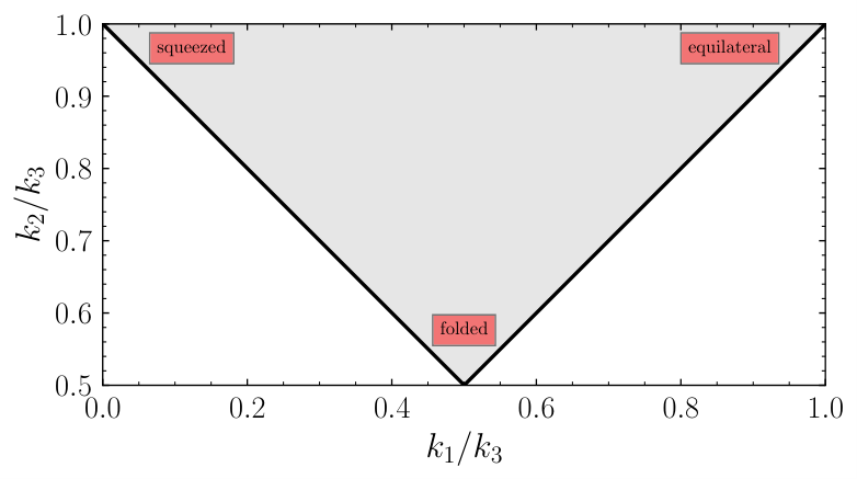
Organizing the momenta as , the conservation of momentum amounts to requiring and : this region is shown in Fig. 3. Given two shapes , one can check that the integral
| (2.31) |
defines a scalar product. Then, the cosine
| (2.32) |
quantifies how much two shapes are similar [3, 4]. It is possible to check that the shape
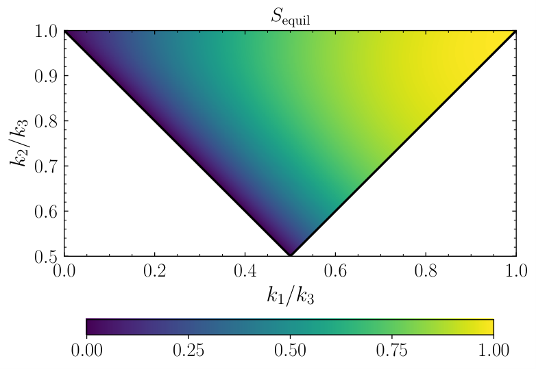
| (2.33) |
has strong overlap with the shape of . This is the equilateral template, which we plot in Fig. 4.
 |
The cosine was originally introduced to study how much two different templates could be distinguished in CMB or large-scale structure data. Given a bispectrum shape, one can build an optimal estimator for its . Then, if two shapes have a small scalar product, the optimal estimator for one shape will be vary bad in detecting non-Gaussianities coming from the other, and vice versa (see Ref. [3] for more details). As such, one could modify the definition of cosine to account for the noise and window function of a given CMB or large-scale structure experiment.
For a comprehensive search, we need a basis of shapes onto which one can project the bispectra of the EFTI [4]. For theories these are the bispectra from and from , whose is
| (2.34) |
The orthogonal shape was introduced for the purpose of obtaining this projection. We plot it in the right panel of Fig. 4.
The orthogonal template takes its name from the fact that it has zero overlap with the equilateral one, . So we can think of it as a second basis vector in the infinite-dimensional space of shapes. Via the cosine we can then obtain and in terms of and .
Constraints on and can then be translated into constraints on the speed of sound and the parameter using Eqs. (2.29), (2.34). This is what has been done with CMB data from the WMAP and Planck satellites [37], and recently from large-scale structure data from the BOSS galaxy survey (see discussion and references in Section 3.12).
Before concluding this section, let us point out a theoretically motivated target for and , following Refs. [5, 6, 54]. These observables are directly related to the cutoff of the EFT: larger means lower strong coupling scale. As discussed in section 2.6, the UV completion of the EFTI has a qualitatively different flavor when , and in particular when . Given the predictions Eq. (2.29) and Eq. (2.34) we see that a natural target is . Much effort has been, and continues to be, devoted to reaching this target.
2.8 Local non-Gaussianity and consistency relations
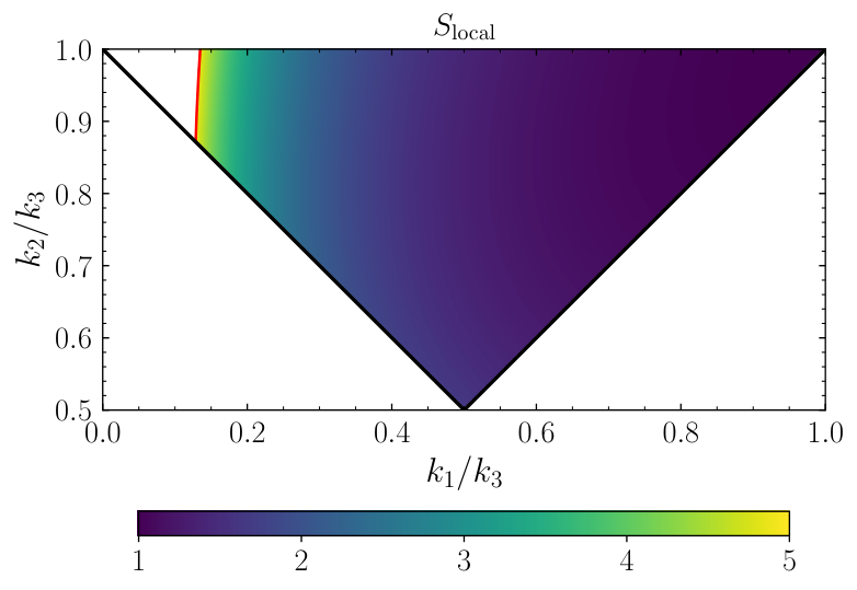
There is another important type of non-Gaussianity, the so-called non-Gaussianity of the local type. Its template is
| (2.35) |
It derives its name from the fact that it comes from a nonlinear local correction to a Gaussian variable: . Importantly, in Fig. 5 we see that it peaks in the squeezed configuration, so it is very distinguishable from equilateral and orthogonal non-Gaussianity.
Local non-Gaussianity vanishes in single-clock inflation. This is a consequence of the fact that in single-clock inflation the squeezed limit of the bispectrum is uniquely fixed in terms of the power spectrum by the consistency relation [7, 8, 45]:
| (2.36) |
where we have defined
| (2.37) |
This result can be derived in the following way. When the long mode goes outside the horizon, the associated perturbations in ADM variables and defined in gauge go to zero. In this limit the metric becomes
| (2.38) |
where we used that becomes a constant. The evolution of short-wavelength modes is then the same as in an unperturbed FLRW Universe, but with a local scale factor . Hence the correlation between the long mode and two short modes is given by a scale tranformation as in Eq. (2.36). Then, we can say that single-clock inflation does not produce local non-Gaussianity: if we measure the squeezed limit of a three-point function, we do not learn anything more than what we would learn from measuring the two-point function. In other words, the long-wavelength field can be locally removed from the metric by a large gauge transformation given by Eq. (2.36), and therefore it is locally unobservable.
Consistency relations for single-field inflation have been an active area of study in the past decade. The main result given in Eq. (2.36) has been generalized for higher-order correlation functions and including soft tensor modes [51, 55, 56, 57, 58], as well as the case of multiple soft limits [59, 60].
The same line of reasoning used to derive inflationary consistency relations can be extended from the horizon exit to re-entry of the long modes. This results in consistency relations for cosmological observables, that all take the form of Eq. (2.36). The more famous are the so-called consistency relations for large-scale structure [61, 62, 63, 64, 65, 66, 67], but similar results have been obtained for CMB anisotropies and CMB spectral distortions [68, 69, 70].
At phenomenological level, consistency relations play a very important role. They imply that any detection of local non-Gaussianity, i.e. a violation of the consistency relations, would rule out all models described by the single-field EFTI. This is why most of the current experimental effort, as far as the physics of the primordial Universe is concerned, is focused on local non-Gaussianity.
2.9 Beyond single-clock inflation
Presence of additional degrees of freedom can significantly modify the predictions of inflation. For instance, inflationary models with extra massless fields (often called “multifield models”) can generate local non-Gaussianity [71, 72, 73, 74, 75]. Therefore, they can violate the single-field consistency condition Eq. (2.36).
In fact, new degrees of freedom even if massive leave their imprints in the squeezed limit of non-Gaussian correlators [76, 77, 78, 79]. For instance, the exchange of a scalar field of mass leads to a squeezed-limit behavior proportional to
| with | (2.39) |
This becomes similar to the local non-Gaussianity as , while there is a distinct oscillatory behavior when . If the exchanged particle had a nonzero spin , then the squeezed limit correlator would also have an angular dependence . Hence by investigating the squeezed-limit of inflationary correlators, we are effectively doing spectroscopy of that era.
Of course, these additional degrees of freedom can be included in the EFTI to reproduce the known results, but more importantly to explore the full range of possibilities that are consistent with the symmetries. Some works along these lines are [80, 81, 82, 83, 84, 85].
To highlight an example, let us recall the Higuchi bound: massive unitary representations of de Sitter group with nonzero spin cannot be arbitrarily light: [86]. This bound suppresses the strength of the squeezed-limit signal coming from spinning degrees of freedom (see Eq. (2.39)). However, even if inflationary spacetime is very close to de Sitter, the Higuchi bound can be strongly violated because dS isometries are broken during inflation (there are preferred time slices). EFT of Inflation helps systematically study this possibility, which indeed leads to phenomenologically interesting signatures [85].
Constraints on primordial non-Gaussianity have been so far driven by CMB experiments, but to improve these constraints we should explore other probes. Chief among these probes is large-scale structure. In order to obtain robust constraints on primordial non-Gaussianity from large-scale structure, however, we must have an accurate theoretical description of nonlinearities from gravitational collapse, since these act as a “noise” for the extraction of the primordial signal. This is where the EFT of LSS, another success in the application of effective field theory techniques to cosmology, comes into play.
3 Effective Field Theory of Large-Scale Structure
The density fluctuations seeded during inflation can be observed through perturbations of the CMB and large-scale structure. Large-scale structure is the distribution of matter on cosmological scales at low redshifts. This distribution is measured through various channels: weak lensing of the CMB and galaxies, spectroscopic galaxy surveys, Lyman- intensity absorption patterns etc. In order to get more information about our Universe one has to establish the connection between these observables and fundamental properties of the Universe. To that end, it is desirable to analyze large-scale structure data just like the CMB, where one uses linear cosmological perturbation theory to extract cosmological parameters from the observed spectra of temperature and polarization fluctuations. However, the large-scale structure observables are somewhat different from the CMB ones. The low-redshift Universe is strongly affected by gravitational instability and complex galaxy formation physics, neither of which can be adequately modeled within linear cosmological perturbation theory. On the other hand, the number of modes available for measurements in large-scale structure experiments is nominally much larger than that of the CMB because the matter distribution is essentially three-dimensional. Potentially, this may lead to very precise measurements of cosmological parameters provided that large-scale structure can be accurately modeled.
The effective field theory of large scale structure [9, 10] and its spin-offs [87, 88, 89] are theoretical tools for accurate analytic calculations of non-linear structure formation in our Universe. The main object of this theory are small fluctuations in the number density of biased tracers, such as galaxies, expanded around homogeneous and isotropic background given by a cosmological model at hand. The cutoff of this theory is given by the scale where the gravitational collapse become very nonlinear or where the impact of astrophysical processes involving baryons is significant. Below this cutoff, the evolution and interactions of the long-wavelength density fluctuations are fixed by gravity as the only long-range force and symmetries of the system. Remarkably, this allows for the description of structure formation on large scales in terms of a weakly-coupled theory, even when the details of complicated baryonic physics governing galaxy formation are unknown. In this way the EFT of LSS provides a direct link between the (non)-Gaussian initial conditions set by inflation and the late Universe observables. In what follows we will review the current state of this field.
3.1 Fluid description of the large-scale structure
In order to illustrate the main principles of the EFT of LSS, we will focus on a simple example where the Universe is dominated by collisionless non-relativistic particles. Such example is already very generic. These particles can represent dark matter, small dark matter halos (as is often the case in numerical N-body simulations) or they can be any other compact objects, such as primordial black holes. Since the gravitation collapse takes place sufficiently inside the Hubble horizon, it essentially occurs in the Newtonian non-relativistic regime. In this regime, the exact description of a system of identical particles of mass which interact only gravitationally is given by the Vlasov equation for the total phase-space probability distribution function (PDF) ,
| (3.1) |
where and are the single-particle gravitational potentials and phase-space densities, and . This setup allows us to obtain the equation of motion for the long-wavelength degrees of freedom by explicitly integrating out the UV modes. This is in practice achieved by coarse-graining the Boltzmann equation by means of a low-pass filter with some cutoff scale and taking the first two moments of the resulting filtered phase-space PDF, which yields [9, 10]
| (3.2) |
In these equations we used conformal time , is the time-dependent matter density fraction which enters the Friedmann equation, is the conformal Hubble parameter, is the gravitational potential and and are the filtered density contrast and peculiar velocity fields, constructed by coarse-graining the density and momentum fields,
| (3.3) |
As argued in [9], consistent truncation of the infinite hierarchy of moments of the Boltzmann equation is possible as long as the scales of interest are larger than the effective mean free path of dark matter particles. Crucially, on the right hand side of the Euler equation in (3.2) we see the appearance of an effective stress-tensor , which is generated by integrating out the short-scale fluctuations. As we will argue shortly, this effective stress-tensor can be expanded in the powers of spacial derivatives and long-wavelength density fields on large scales. Therefore, the fluid description of our Universe is possible as long as the following condition is satisfied
| (3.4) |
where is a wavenumber of density perturbations and (at redshift zero) is the so-called nonlinear scale for which the variance of the density field becomes of order unity: .
Eq. (3.2) is the equation of motion for the long-wavelength degrees of freedom. We have obtained it starting from a simple exact description of a self-gravitating system and explicitly integrating out the UV modes. However, as in any other EFT, the same equations of motion can be derived identifying the relevant long-wavelength degrees of freedom and imposing all symmetries of the system [90], even when the UV model is unknown. Therefore, the long-wavelength description given by Eq. (3.2) is universal, i.e. by construction it covers all possible microscopic scenarios of structure formation. This description allows one to capture effects of unspecified UV physics in a systematic and robust fashion. This is not surprising, given that the EFT decoupling principle guarantees that the impact of any UV physics can be captured by effective operators constructed from the long-wavelength degrees of freedom only.
3.2 Stress tensor and (non–)locality in time
Filtering short-scale modes produces an effective stress-energy tensor in the Euler equation Eq. (3.2). This tensor depends only on the long-wavelength degrees of freedom, i.e. the smoothed density contrast and peculiar velocity. These two fields contain deterministic and stochastic components. The deterministic component is correlated with the long-wavelength fields, while the stochastic is not. However, its statistical properties are strongly constrained by symmetries, i.e. the presence of the stochastic component still allows the theory to be predictive.
On sufficiently large scales the non-linear evolution is negligible, and hence these quantities are small. Thus, the deterministic part of the effective stress-tensor can be Taylor-expanded in powers of the wavenumbers and the large scale fields and spatial derivatives. The most general expression consistent with the rotation invariance and the equivalence principle is given by [91]
| (3.5) |
where is a time propagator, is the position of the fluid element at time . We emphasize that the effective stress tensor depends on fields evaluated on the past light-cone, i.e. the EFT of LSS is in general nonlocal in time [92]. In conventional effective field theories the time scale of short modes is faster than the time scale of long-wavelength degrees of freedom, in which case their evolution can be approximated as quasi-instantaneous, i.e. quasi-local in time. However, in the context of LSS both short and large scales evolve on the same characteristic timescale . Nevertheless, in perturbation theory the fields in the right hand side of Eq. (3.5) can be Taylor-expanded around the fluid trajectory such that the theory can be reformulated in terms of local-in-time operators. Thus, the effective stress tensor at next-to-leading order is given by [10, 91, 93, 94, 95]
| (3.6) |
where , are time-dependent Wilson coefficients, and we have introduced the tidal tensor as
| (3.7) |
The general basis of counterterms at higher orders involves convective derivatives [93, 96, 97], which come from expanding in Eq. (3.5). is the stochastic contribution which is uncorrelated with . It is local and analytic in space and obeys the equivalence principle, as well as the mass and momentum conservation. At the lowest order it is given by
| (3.8) |
3.3 Loop expansion
Plugging (3.6) into (3.2) we obtain effective equations of motion of the matter fluid. At linear order in it solved by the linear growing mode
| (3.9) |
where is the initial density field and is the linear growth factor normalized to unity at zero redshift, is the logarithmic growth factor. The initial conditions for structure formation are set after recombination, such that is a nearly Gaussian random field, whose properties are encoded in the linear power spectrum :
| (3.10) |
such that at leading order (in linear theory) we have
To solve Eq.(3.2) it is convenient to work in the EdS approximation, and to split the fields of interest and into two parts.44 4 In cosmological perturbation theory only the longitudinal part of has a growing mode. The transverse part decays in linear theory but gets excited at the non-linear level. In principle, it can be taken into account, but its contribution is negligible for most applications [90]. One part is obtained upon formally setting the effective stress tensor to zero, while the other part will include corrections due to the presence of this tensor. This way the total perturbative solution for the matter density can be written as
| (3.11) |
and similarly for the velocity divergence . The corrections are given by
| (3.12) |
where are certain convolution kernels whose form is dictated by the non-linear structure of the pressureless fluid equations. Explicitly for the first three kernels we have:
| (3.13) |
The first correction generated by the stress-tensor is given by
| (3.14) |
where is the density field Green’s function of the linearized fluid equations [10]. The two-point function of the matter field including leading order non-linearities (i.e. one-loop corrections) is given by with
| (3.15) |
This correction admits a representation in terms of Feynman diagrams shown in Fig. 6.
The split of the perturbative solution (3.11) is useful for the EFT power counting. On mildly-nonlinear scales the linear power spectrum can be approximated as a power-law with [99, 90]. Using the approximate Lifshitz symmetry the dimensionless power spectrum can be written as,
| (3.16) |
where the first line contains one-loop corrections produced by the intrinsic non-linearity of the fluid equations, while the second line displays the terms coming from the deterministic and stochastic parts of the effective stress tensor. The two-loop corrections scale as
| (3.17) |
which indeed confirms that at NLO we only need to keep the effective operators with Wilson coefficients and . Note, however, that the actual power spectrum of our Universe is not a power-law. In particular, it has the BAO wiggles, which break the naive power counting in and require a special treatment within a procedure called IR resummation.
3.4 UV renormalization and IR resummation
The UV limit of the one-loop integral in Eq. (3.15) reads
| (3.18) |
At face value, UV modes couple to modes with mildly-nonlinear wavenumbers /Mpc through the variance of the short mode displacement field. We see that this integral diverges for a generic initial power spectrum. This divergence is exactly canceled by the Wilson coefficient , which ensures that the physically observed quantities such as the density field n-point correlation functions are finite. Their dependence on short-scale physics is captured by the finite part of , which can been accurately measured in N-body simulations [10, 100, 98, 101] or can be inferred from the data.
The IR limit of the one-loop integral reads [102, 103]:
| (3.19) |
If the linear power spectrum did not have any feature i.e. , such that , the differential operator above could be Taylor-expanded and we would find that the IR modes couple to a mildly-nonlinear mode though the variance of the large-scale density field [104, 105, 106, 107, 65],
| (3.20) |
This coupling is rather weak. However, contains BAO wiggles, whose coupling to IR modes is enhanced. Approximating with , ( Mpc is the comoving acoustic horizon at decoupling) we obtain
| (3.21) | ||||
The integral receives contributions from modes all the way up to , and it is numerically close to the large-scale variance of the displacement field, which turns out to be quite large, i.e. at for modes of interest /Mpc. Hence, the higher order soft loop corrections to (3.21) are not negligible and must be resummed for the correct description of the BAO. This procedure is called “IR resummation” [108, 102, 103, 109, 11, 110, 111, 112]. It was originally formulated within the Lagrangian effective field theory, but shortly it was shown that IR resummation can be performed directly at the diagrammatic level within the Eulerian EFT [103, 111]. At zeroth order in hard loops (with ) one has
| (3.22) |
3.5 Flavors of the EFTs
It is important to stress that at the technical level, there are several different ways to realize the EFT of LSS ideas. The original proposal of the EFT in Eulerian fluid variables that we have discussed so far is plagued by the large IR contributions that require IR resummation. IR resummation in terms of Eulerian fluid variables is complicated by the presence of the spurious IR enhancements in the loop diagrams. This motivated the development of the Lagrangian EFT of LSS [87, 89, 109, 113, 114, 115, 116]. The Lagrangian EFT of LSS also partially resums some of the UV contributions. From the computation efficiency point of view, however, it is still beneficial to work in Eulerian space. In this case it is still possible to perform a systematic IR resummation, as discussed in Sec. 3.4, which is particularly manifest within a path integral formulation of the EFT of LSS known as Time-Sliced Perturbation Theory [88, 103, 111, 117]. All these different techniques agree within the overlapping domains. This reflects the uniqueness property of the EFT: the predictions for physical processes do not depend on a particular formulation, once the results are compared to the same order in appropriate small parameters. In other words, at a given order in relevant IR and UV small parameters, the difference between the EFT formulations appears only at higher orders.
3.6 Biased tracers
So far we have discussed the clustering of pure matter. The galaxy density field observed in cosmological surveys is a biased tracer of the underlying dark matter field. The relationship between them is given by a past light-cone integral over local long wavelength perturbations of matter density, velocity, and tidal fields [118, 96, 119, 120, 121, 122],
| (3.23) |
where is a random field uncorrelated with , which captures the stochasticity of the tracer, are time-dependent kernels with characteristic timescale and order-one amplitudes, i.e. , is the typical length scale of the object. Just like in the case of the effective stress-tensor of matter that we discussed above, the apparent non-locality in time in Eq. (3.23) can be removed in perturbation theory by Taylor-expanding around the fluid trajectory, which allows one to rewrite the bias relation as a local-in-time expression [119]55 5 Strictly speaking, it is possible to rewrite the bias expansion in the local-in-time form only in the so-called Einstein-de-Sitter approximation for the time evolution [121], which is accurate for redshifts relevant to current and future surveys. For works dealing with exact time dependence, see for example [123, 124, 125].
| (3.24) |
where is the stochastic field uncorrelated with the long-scale perturbations, and we have introduced new Galileon operators
| (3.25) |
( is the velocity potential), and “” denote both the operators which do not contribute to the one-loop power spectrum after renormalization and higher order operators. Free parameters are time-dependent Wilson coefficients. In the cases where the bias tracers are galaxies or dark matter halos, these bias parameters, up to quartic order, have already been detected in simulations, see e.g. [126, 127, 121, 128, 129, 130].
Importantly, the bias expansion has a new UV scale , which can be associated with the typical size of the collapsed object [96, 118, 121, 129]. For halos this has the order of magnitude of the Lagrangian radius of the overdensity clump that collapses into a host halo. For the line emission this has the order of the Jeans scale of the diffuse gas [121, 131]. For galaxies depends both on the host halo properties and on the details of galaxy formation, e.g. the ambient radiation field and thermal heating of intergalactic medium.
Another important difference compared to the dark matter case is that the power spectrum of the stochastic field does not fall off on large scales as in Eq. (3.8), but it is rather constant as goes to zero. This is a consequence of the fact that for biased tracers mass and momentum are not conserved, given that each galaxy is counted the same, regardless of the mass of the host dark matter halo. This constant power spectrum of the stochastic field is related to the well known Poisson noise for biased tracers.
3.7 Redshift-space distortions
When galaxy surveys map the Universe they assign the radial position of galaxies according to their redshifts. The observed galaxy redshift is contaminated by peculiar velocity projections onto the line-of-sight, which gives rise to redshift-space distortions (RSD). From the EFT point of view, RSD boil down to the following velocity-dependent coordinate transformation
| (3.26) |
where denotes the line-of-sight direction and we have employed the plane-parallel approximation valid on short scales. Taylor expanding the exponent in the RSD mapping and coarse graining the resulting composite operators involving various insertions of velocity fields one obtains a set of new Wilson coefficients which properly renormalize the UV sensitivity of the redshift-space density. Thus, the redshift-space mapping is an additional source of non-linearity which can be consistently taken into account within the EFT [132, 133, 11].
3.8 Baryons in the EFT of LSS
One particularly compelling advantage of the EFT framework for LSS is that it is possible to include analytically the effects of small scale baryonic, or star-formation, physics on large-scale clustering [134, 135]. In this approach, one treats the CDM and baryons as separate fluids coupled through gravity, each with its own set of EFT parameters which capture the UV properties of the system. The functional form of these effects on large scales, i.e. as a function of , is fixed by symmetries and organized in a controlled derivative expansion, just like the the pure CDM case described above. For predictions on large scales, this can be a significant advantage over relying on -body simulations that include baryonic processes. This is because, unlike the case for pure CDM, we do not know a priori the short-scale baryonic physics that should be included in the simulations.
As an example, [135] used this approach to compute the CMB lensing potential and compare with a numerical simulation (see Fig. 7), which shows quite good agreement up to . This is an important observable because it can be used to probe neutrino masses in CMB-S4, and much of the constraining power for a mass sum of less than comes from [136].
3.9 EFT of LSS at the field level
So far we have been focusing on calculation of correlation functions. However, the EFT of LSS naturally predicts the full non-linear density field, given some realization of the initial conditions. This can be exploited in two ways.
First, the field-level predictions provide a natural way to compare the theory to numerical simulations. If they share the same initial conditions, the comparison can be done without paying the price of cosmic variance. Furthermore, such comparison is much more stringent since one has to fit all Fourier modes and not only the summary statistics. This has been exploited in the past to provide the first reliable measurements of the EFT parameters and the nonlinear scale [137, 138] as well as for the detailed comparison of theory and simulations for biased tracers in real and redshift space [139, 140].
Second, these methods can be used to construct the field-level EFT likelihood in the perturbative forward modelling. Such approach aims at measuring cosmological parameters from the full nonlinear field, without using summary statistics. A lot of progress has been made recently towards achieving this goal, see for instance [141, 142, 143, 144, 145, 146, 147, 148, 149].
Finally, some progress was made recently in fixing the form of galaxy correlation functions using only symmetries of the system and the equivalence principle, without explicitly relying on the equations of motion. This is inspired by the similar cosmological bootstrap approach to derive the form of inflationary correlators from symmetries and general principles such as locality and unitarity. The natural starting point for this “LSS bootstrap” is at the field level, where various theoretical constraints can be straightforwardly imposed [150, 151].
3.10 Extensions
Other important extensions of the EFT include the incorporation of non-Gaussian initial conditions [133, 120, 152, 153], IR-resummation of primordial oscillating features [117, 154, 155], and an accurate treatment of massive neutrinos. The later is a conceptually challenging task, as the neutrino free-streaming scale is significantly longer than the non-linear scale . However, massive neutrinos can be split into “fast” and “slow” ones, which allows to identify a small parameter in the regime and systematically compute their effect on dark matter clustering [156, 157].
Another important task is to account for selection effects, which may be present in realistic surveys. The effective operators capturing these effects at leading orders are given in Ref. [158]. The extensions for CMB lensing, galaxy lensing, and intrinsic alignments are worked out in Refs. [159, 160]. The incorporation of additional degrees of freedom associated with dark energy and modified gravity was done in Refs. [161, 162, 163, 164, 165, 166] and is described in more detail in Sec. 4.
3.11 State-of-the-art computations
The state-of-the-art EFT calculations that have been carried out up to now are listed in Table 1, see Refs. [91, 107, 100, 167, 95, 168, 169, 170, 171, 172, 173]. These calculations must be extended to higher loop orders and higher -point functions in order to use more observed modes in cosmological data analyses. The consistent inclusion of massive neutrinos has been done for the one-loop power spectrum and tree-level matter bispectum [156, 157]. The results of IR resummation formally exist for an arbitrary n-point function and for an arbitrary number of hard loops both in real and redshift spaces and for a generic biased tracer [111].
| Type | Power spectrum | Bispectrum | Trispectrum |
|---|---|---|---|
| Matter in real space | 3-loop | 2-loop | 1-loop |
| Biased tracers in real space | 1-loop | 1-loop | — |
| Biased tracers in redshift space | 1-loop | 0-loop | — |
It is worth mentioning that the computation of EFT loop corrections requires efficient numerical tools to evaluate perturbation theory convolution integrals. These techniques are necessary in order to apply the EFT calculations to observational data. FFTLog is one of such techniques [174, 175, 176]. It has been worked out to one-loop order for biased tracers in redshift space [177], for the two-loop power spectrum and the one-loop bispectrum for matter in real space [176], and for BAO resummation in [112].
3.12 Applications to current and future data
The EFT of LSS allows one to take advantage of the cosmological information encoded in the full shape of the observed galaxy power spectrum. This means a consistent analysis of the large-scale structure data that includes fitting fundamental cosmological parameters directly from the power spectrum shape, as it is routinely done in cosmological analyses of the CMB.66 6 This can be contrasted with the nomenclature of some previous works, which used the term “full shape” for an analysis which studies how a particular fixed power spectrum template gets distorted by the Alcock-Paczynski effect [179]. This analysis has been done for the first time in Refs. [12, 13], which showed that galaxy power spectrum measurements from the Baryon acoustic Oscillation Spectroscopic Survey (BOSS) data release 12 [180] is a powerful source of cosmological information.
EFT-based analyses of the BOSS data yield the CMB-independent measurements of the parameters of the base CDM model and its extensions [181]: the Hubble constant , the current matter density fraction , the primordial power spectrum amplitude and tilt , the mass fluctuation amplitude , as well as constraints on the spatial curvature of the Universe , and the dark energy equation of state parameters [183, 184, 185, 186, 178, 187, 188, 182, 189, 14]. Remarkably, many of these parameters are measured with precision similar to that of the Planck CMB data results, e.g. and , see Fig. 8. Besides, combining the EFT-based full-shape BOSS likelihood with the CMB data has lead to new constraints on the total neutrino mass, effective number of relativistic degrees of freedom [190]. Moreover, the new BOSS likelihood allowed one to derive new constrains on certain models addressing the so-called “Hubble tension.” The use of the EFT-based likelihood was crucial in order to show that such models are ruled out by the current large-scale structure data [191, 192].
In addition, another exciting development has been the application of the EFT of LSS to constrain primordial non-Gaussianities (see Sec. 2.7) [15, 16], including the first-ever bounds on single-field primordial non-Gaussianity from galaxy surveys. Local-type non-Gaussianity, typical for multifield models, has been constrained using the scale-dependent bias of the power spectrum in, for example, [193, 194, 195].
The sensitivity forecasts for ongoing experiments such as Euclid and DESI suggest that the application of the EFT to these surveys can lead to significant improvements in cosmological parameter measurements [196]. This includes a -detection of the sum of neutrino masses and measurement of the Hubble constant from the combination of the Planck CMB and Euclid/DESI data. Also, recent constraints on non-Gaussianity suggest promising and competitive results in the future, given the volume of ongoing state-of-the-art surveys and the ability of EFT formalism to provide more precise computation of relevant observables. These conclusions are based on a realistic analysis including marginalization over all necessary Wilson coefficients and data cuts consistent with the theoretical error [197], which is determined by calculations that are available at present. The results are expected to improve with more precise calculations and with better priors on Wilson coefficients, which can be obtained from high fidelity numerical simulations [198]. Indeed, these types of analyses, and their higher-precision versions of the future, were one of the main motivations for the development of the EFT of LSS.
Looking beyond this decade to the next generation of high-redshift spectroscopic surveys, an increase by another order of magnitude in the number of observed galaxies is expected (for example, see the snowmass white paper on opportunities of high-redshift and large-volume future surveys [199] and references therein). In this coming era of the ultimate precision, the EFT methods discussed here will be even more valuable.
4 Effective Field Theory of Dark Energy
Observationally speaking, Einstein’s theory of General Relativity (GR), as far as we can tell, successfully describes gravitational and cosmological phenomena over an enormous range of length and time scales. For example, GR describes small effects in our Solar System, such as the precession of the perihelion of Mercury and the bending of light around the Sun, it describes large effects like the expansion of the Universe, both at early and late times, it describes gravitational-wave emission by binary inspirals, and it describes black holes. The broad applicability of GR, however, is (most likely) not simply a convenient accident. GR is the unique low-energy Lorentz invariant theory of an interacting massless spin-2 particle (see e.g. [200, 201]), and gauge invariance of the action implies that all other fields couple to gravity with the same strength (this is called the equivalence principle, see e.g. [202]). These facts make the predictions of the universal, long-range force quite robust.
The standard cosmological paradigm, describing the large-scale evolution of the Universe from the moments after the Big Bang until the current time, is GR with a cosmological constant coupled to a fluid-like system of cold dark matter (CDM) particles, called CDM. This model so far successfully describes cosmological phenomena such as the cosmic microwave background, Big Bang nucleosynthesis, the large-scale structure of the Universe, and gravitational lensing of galaxies, to name a few.
A historically theoretically worrying critique of the CDM paradigm, though, is the cosmological constant problem. This is the fact that the observed value of the background energy density is 60 to 120 orders of magnitude smaller than what is expected from our understanding of particle physics, and seems to represent a huge fine-tuning problem for the theory [203]. In response to this problem, Weinberg suggested the compelling anthropic solution [204, 205]. His argument roughly goes like this. First of all, viewing GR as a low-energy effective field theory, the cosmological constant is the most relevant operator, and so is generically expected to be present in the low-energy theory, although its value is not known a priori. In order to estimate its value, Weinberg pointed out that if it were much larger than the current observed value, there would be no stars or planets (and therefore no humans) in the Universe. Thus, if there are many patches of the Universe with different values of (for example, in a multiverse scenario), then humans would only exist in the patches with small values of .
This then brings us to dark energy (DE) and modified gravity theories,77 7 For the purposes of this review, we do not make a meaningful distinction between DE and modified gravity theories. which are essentially attempts to change the low-energy dynamics of gravitation. Historically speaking, these theories were considered, in part, as potential explanations for various perceived theoretical shortcomings of GR, such as in the Brans-Dicke theory [206] and early quintessence models [207]. Theories of DE and modified gravity attempt, among other things, to solve the cosmological constant problem88 8 Although no compelling solution has yet been found. or explain the acceleration of the Universe without an explicit cosmological constant (so-called self-accelerating solutions, see for example [208]). While the history of motivations to study extensions to GR (see [209] for example for a review) is important, we prefer to take a slightly different perspective in this review, one more in line with the EFT principles that we have been discussing. Here we simply ask what are the possible observable deviations from CDM? The question in this form has the advantage that it points us toward systematic ways in which we can test GR and look for deviations caused by new physics, which is especially relevant in this era of precision cosmological measurements.99 9 Upcoming observations range from galaxy surveys like the Rubin Observatory (formally LSST), Euclid, and DESI, to CMB measurements with CMB-S4, to 21cm emission measurements with SKA, to measurements of gravitational waves with LIGO/Virgo, together representing billions of dollars of international investment.
4.1 Unitary-gauge action in the presence of matter
In this review, we focus on modifications to CDM arising from an extra scalar mode which is related to the breaking of time diffeomorphisms in the Universe (i.e. the presence of the preferred slicing of space-time where the CMB is nearly homogenous and isotropic). As discussed above in Sec. 2.1, a general way of describing all such possible modifications is to write the action for the metric in unitary gauge. Instead of demanding that the action be diffeomorphism invariant, we demand that it be invariant under time-dependent spatial diffeomorphisms. Since the action has less symmetry, there is an extra scalar degree of freedom in addition to the normal two degrees of freedom of the graviton, and the scalar mode can be made manifest by performing the Stueckelberg trick. In fact, this procedure is exactly the same as the one discussed in Sec. 2.1 for the EFTI, with the only difference now being that, because we want to describe late-Universe physics, we have to include the coupling of the metric to matter.
The full action is made up of a gravitational part , and a matter part ,
| (4.1) |
In terms of covariant objects like the Riemann tensor and the covariant derivative , as well as time-diffeomorphism breaking operators like and the extrinsic curvature , the gravitational action has the form [1, 2, 17]
| (4.2) |
Here, the index ‘’ referrs to the time coordinate which parameterizes equal-time surfaces. The matter action can also in principle depend on all of the aforementioned fields and the matter fields, , coupled in such a way that allows operators which break time diffeomorphisms. Thus, the generic form is (see [80] for example)
| (4.3) |
with the same rule that for any covariant object, it is allowed to appear with an upper index. Once the action is written in this way, the Stueckelberg trick can be used to introduce the scalar mode just as in Eq. (2.12), for example.
In this review, we assume the existence of a frame, called the Jordan frame, where each matter species is minimally coupled to the same metric. Then, the action in the Jordan frame in unitary gauge reads
| (4.4) |
where is as in Eq. (4.2), but is fully diffeomorphism invariant. For the matter action, we can write
| (4.5) |
where for pressureless CDM, we have
| (4.6) |
where is the energy density in the rest frame of the fluid, and is the fluid four-velocity. In the non-relativistic limit, we have
| (4.7) |
and we have introduced the background energy density , the overdensity and the fluid three-velocity .
Similar to Eq. (2.3), we can write the gravitational action as
| (4.8) |
where the explicit operators shown are the only ones that contain linear perturbations, while contains terms that start quadratic in the fields. Furthermore, is constant and is related to the effective Planck mass by Eq. (4.14) below. The presence of the function above differs from the inflationary case, where, since there is no matter, one can always eliminate through a redefinition of the metric. From Eq. (4.5) and Eq. (4.8), we can then find the background equations (i.e. to cancel the tadpole terms) which are given by [17]1010 10 We assume zero spatial curvature of the background FLRW metric throughout for simplicity.
| (4.9) | ||||
which reduce to the inflationary relations Eq. (2.4) when , , and . Once the background equations have been determined, the differences among DE theories is contained in .
At this point, in order to generate the most general DE models, one could simply write all of the possible terms in invariant under time-dependent spatial diffeomorphisms, organized in a derivative expansion, much like in Eq. (2.3). However, many DE models in the literature focus on a specific subset of operators, motivated by the following considerations. First of all, the scale associated with the observed background expansion is
| (4.10) |
Then, because GR has been stringently tested on Solar System scales, one typically tries to set up a screening mechanism (for example Vainshtein screening [210, 211]), so that GR is recovered on smaller scales, but gravity is modified on larger cosmological scales. The Vainshtein mechanism relies on large nonlinear terms in the action which leads to a second scale defined by
| (4.11) |
(which is roughly the Vainshtein radius for a Planck mass) and leads to Galaxy size screening for the Sun, for example. Thus, we will consider interactions in the EFT which are suppressed by this much smaller scale .
While promoting these nonlinear interactions, higher-derivative terms can generically appear in the equations of motion, which can lead to unstable Ostrogradski ghosts (see [212], for example). To get around this, it is common to consider models which explicitly only contain second derivatives in the equations of motion (Horndeski theories [213, 214]), or that contain higher derivatives, but have a degenerate kinetic structure so that only one extra, non-ghost, scalar mode propagates (beyond Horndeski, Gleyzes-Langlois-Piazza-Vernizzi (GLPV), and degenerate higher-order scalar-tensor (DHOST) theories [215, 216, 217, 218, 219, 220]). The specific choices of nonlinear terms in these theories is protected from large quantum corrections by a weakly broken galileon invariance [221, 222]. Finally, for everything we discuss in this review, we will be working in the Newtonian limit, where , so we will only consider the leading operators in this limit.
With these considerations in mind, a quite general EFT action for the tensor and scalar modes is (for GLPV theories, see [18] and references therein)
| (4.12) |
with
| (4.13) |
where is the three-dimensional Ricci tensor of the equal-time hypersurfaces and the time-dependent effective Planck mass is given by
| (4.14) |
For example, Horndeski theories have and . It is sometimes convenient to express the above EFT parameters as dimensionless parameters that are expected to be ,
| (4.15) | ||||
For example, changes the speed of tensors to [223]
| (4.16) |
These dimensionless parameters also allow us to easily estimate the scales suppressing various interactions. One can show that, in terms of the canonically normalized scalar field , we have for example
| (4.17) |
so that this interaction is suppressed by , as desired. Because is the scale suppressing the interactions, it is often referred to as the unitarity cutoff of the EFT.
We would like to mention that a lot of work has been done on scalar-tensor theories in the covariant formulation, where one starts with a covariant action and then expands around the background [213, 224, 214, 225, 218, 219, 220],1111 11 For a relationship between the EFT parameters in Eq. (4.12) and a covariant formulation, see [226], for example. but in the spirit of this review, we would like to mention a few advantages of the EFT formulation. On the theoretical side, the EFT approach is agnostic as to what kind of fundamental physics gives rise to the low-energy dynamics; the action Eq. (4.12) could indeed come from a fundamental scalar field, but it could also be the low-energy action of the longitudinal mode of a massive vector field, for example. On the practical side, once the background is fixed as in Eq. (4.9), the EFT is directly an expansion in the perturbations, and so the independent free parameters are more easily identified.
4.2 Linear cosmology
Before matter starts to clump into structures, the Universe is well approximated by a homogenous expanding background with coupled linear perturbations of all of the relevant fields. In the early Universe, this includes photons, neutrinos, baryons, and dark matter, for example. As the Universe cools, non-relativistic matter starts to dominate the dynamics, and the dark matter starts to fall into larger and larger potential wells. When the dark-matter overdensity reaches , the evolution enters the non-linear regime.
The linear regime holds through the CMB until the early times of matter domination. This means that both CMB observables and the initial conditions for LSS can be computed with linear theory. In this section, we discuss some modifications of CMB and linear LSS observables that result from the EFT of DE, see for example [227, 228, 229, 230, 231, 232, 233, 234, 235, 236, 237, 238, 239, 240, 241, 242, 243, 244, 245].
In Newtonian gauge, one can write the scalar part of the metric as
| (4.18) |
where and are the gravitational potentials. Some early attempts to describe deviations from CDM included the phenomenological functions and , which parameterize changes in the Poisson equation
| (4.19) |
and the anisotropic stress
| (4.20) |
where in CDM. The EFT of DE, however, provides a systematic way to compute relationships like these from a consistent theory in a controlled derivative expansion, specifically allowing one to see if certain parameters enter multiple observables. For example, varying Eq. (4.8) with respect to , , and in the quasi-static limit gives the equations relevant for large-scale clustering, which has a solution like that shown in Eq. (4.30). These equations, in addition to the evolution equations for the fluid, are directly relevant for the non-relativistic evolution of the matter overdensity . An analogous relativistic set of equations can also be found, which is relevant for CMB anisotropies [241].
As examples of DE effects, in Fig. 9 and Fig. 10, we show results from [241] for the modification of the matter power spectrum and the CMB, respectively, with , for various values of , the present-day value of . The effect of is sometimes referred to as ‘kinetic matter mixing,’ or KMM, because it results in a kinetic coupling between matter and the DE field . In this case, we can see that larger values of tend to suppress the matter power spectrum on small scales, suppress the CMB lensing power spectrum, and increase CMB anisotropies at small multipoles. A number of publicly available codes have been developed to solve the linear Boltzmann equations with DE [228, 235, 244].
4.3 Gravitational wave propagation
Given the explosion of measurements of GW signals coming from binary inspirals after [246], one important question is how the DE action Eq. (4.12) affects GW propagation. As we have already seen in Eq. (4.16), the speed of the graviton is changed by the operator , proportional to . However, the observation of GW170817 and its electromagnetic counterpart GRB170817A [247] constrains the speed of gravitational waves to be the same as the speed of light to within approximately , i.e.
| (4.21) |
Subsequent works used this fact to significantly constrain DE models [18, 19, 20, 248]. In the language of this review, Eq. (4.21) constrains the EFT of DE to have , which for all intents and purposes means that
| (4.22) |
As [18] also pointed out, in order for Eq. (4.21) to hold also for small changes in the cosmological background (i.e. if the matter fraction were slightly different in our Universe), the EFT of DE action Eq. (4.12) must also have
| (4.23) |
So we see that these kinds of cosmological observations can have dramatic implications for the allowed operators in the EFT of DE.
Apart from the graviton speed, we can also use GW observations to constrain some other non-linear DE interactions. Assuming the previously mentioned constraints Eq. (4.22) and Eq. (4.23), the DE action Eq. (4.12) contains the term , which leads to the interaction vertex
| (4.24) |
between the canonically normalized graviton and scalar field [226], where the scale suppressing the interaction is given by
| (4.25) |
This cubic vertex allows the graviton to decay, through the diagram in Fig. 11, into two scalar modes when , where is the speed of sound of the scalar.1212 12 This decay is allowed for because Lorentz invariance is spontaneously broken by the background evolution. Calling the decay rate of the graviton, and demanding that gravitons do not decay over cosmological distances (since in fact we see gravitational waves), we have and one obtains the strong constraint [226]
| (4.26) |
which alternatively means
| (4.27) |
in GLPV theories.1313 13 For DHOST theories which have the extra parameter , the constraint becomes .
The interaction vertex Eq. (4.24) also modifies the dispersion relation , i.e. the dependence of the energy on wavenumber, through the Feynman diagram in Fig. 11, which is also constrained by GW measurements [249, 246]. This interaction leads to a modification of the graviton dispersion relation [226]
| (4.28) |
where is an arbitrary renormalization scale, and is a small positive parameter. The decay rate and the modified dispersion above are indeed connected by the optical theorem
| (4.29) |
where the sign of is important to have the correct branch cut of the . Current observations limit the above deviation from to a similar level as in Eq. (4.26) [226].
While the above discussion focused on the perturbative quantum mechanical decay of the graviton, the GWs that we measure are actually classical waves with large occupation numbers, a fact that tends to further increase instabilities through Bose enhancement [250]. As discussed in [250], the regime of narrow resonance, where the computation is under analytic control, is able to probe for LIGO/Virgo type measurements, and for a LISA type experiment. Further study of classical effects [251] showed that GWs can induce instabilities in the scalar field throughout the Universe unless and , thus providing even stronger constraints on the EFT of DE.
Before closing this section, we should mention a few potential caveats to the above discussion. First, since the momentum of observed GWs is close to the unitary scale of the EFT of DE (whose actual UV cutoff could be lower), the EFT may not actually be valid on those scales, and the above constraints would not apply [252]. Additionally, positivity arguments suggest that a theory with an approximate Galilean symmetry (the term in the EFT of DE) would have to break down at a cutoff of approximately [253], and so again, the above constraints would not apply. Exceptions to this conclusion in the above discussion could be the constraints obtained in [251], which are relevant for GW frequencies of approximately .
4.4 Large-scale structure
To study effects at much smaller energies, well below the unitary cutoff , we can turn to LSS, where the inverse length scale associated to the non-linear scale is , well below even the scale of current GW measurements. Thus, LSS constraints on DE would be much more relevant if for some reason the EFT of DE breaks down near GW scales.
In this review, we focus on DE effects in LSS in the mildly non-linear regime, and as always, we assume the Newtonian limit (). To see how DE affects LSS, we start with a CDM fluid Eq. (4.5) coupled to DE through Eq. (4.1). DE is then described by the action Eq. (4.12), and in this section, we assume the Horndeski limit. In this case, the form of the fluid equations is the same as in Eq. (3.2), including the stress tensor .
The effects of DE in Eq. (3.2) come in through the modified Poisson equation, and the terms relevant for the one-loop power spectrum are (we use the scale factor as the time variable)
| (4.30) | ||||
where the are functions of time, and are explicitly given in [162] in terms of the EFT of DE parameters in Eq. (4.15), and we have used the notation
| (4.31) |
Furthermore, the momentum dependent interaction vertices describing the effects of DE are given by1414 14 Notice that in terms of the standard mixing functions and , we have (4.32)
| (4.33) |
For example, the second-order solution for (which is relevant for the one-loop power spectrum and the tree-level bispectrum, for example) has the form [254, 255, 256, 257, 258]
| (4.34) |
where
| (4.35) |
and the are functions of time which involve integrals over Green’s functions of the linear equations of motion. As discussed in [163], the function depends on the non-linear modification , and and are changed from their CDM values by the linear modification .

At this point, a few comments are in order. First of all, we stress the inclusion of the stress tensor from the EFT of LSS. Since the fluid mass and momentum are conserved in Horndeski theories, the counterterms in take the same form as in CDM Eq. (3.6), so that the term relevant for the computation of the one-loop power spectrum is [163]
| (4.36) |
where is an unknown function of time that depends on the details of short-scale clustering. The scale above is the non-linear scale of structure formation, which in the presence of DE can be different from the corresponding scale in CDM [163]. The scale is also different from the so-called Vainshtein scale (discussed more in the next section), which is the scale at which the non-linear terms in the equations for the scalar field become important [259]. In the limit that , Vainshtein screening takes place on scales much smaller than gravitational non-linearities and we would expect to only see linear modifications of gravity near . On the other hand, if , then scalar field non-linearities become important on scales much larger than those we typically use in LSS, causing the perturbative expansion assumed in this section to break down on larger scales. Thus, the regime is the one in which we would expect to see new features in non-linear clustering due to DE [162].
As mentioned in Sec. 3, the advantage of the EFT of LSS is that one can perform precise, controllable, and improvable fits to clustering data, and as we have seen in this section, it is also the natural framework to include physics beyond the standard CDM paradigm. Work using the EFT of LSS to compare to simulations including DE was started in [164]. For inclusion of a clustering quintessence DE model in the EFT of LSS, see [161, 124], and for works on structure formation with DE outside of the context of the EFT of LSS, see for example [260, 261, 262, 263].

4.5 Violation of the consistency relations of LSS
The final topic that we will mention in this section concerns the consistency relations of LSS [61, 62, 63, 64, 65, 66, 67]. These are general, non-perturbative relations satisfied by LSS observables in various “soft” limits (when some momentum is taken much smaller than others). For example, the consistency conditions are the reason that the coefficient of is not modified in Eq. (4.35) for Horndeski theories [165] (a similar result holds for clustering quintessence theories [124]). In GLPV and DHOST theories of DE, however, the consistency relations are violated [165, 166] (see also [264, 265]), essentially because the scalar field introduces a large-scale relative velocity which cannot be removed by a coordinate transformation. The violation of the consistency relations in DHOST theories is proportional to the relative velocity, and is computable in terms of parameters of the linear theory [166]. For example, the one-loop power spectrum in DHOST theories has the form
| (4.37) |
where is a parameter proportional to the DHOST parameters or , and is proportional to the large-scale relative velocity [166]. In CDM, IR dominant terms like Eq. (4.37) are not present in the loop expansion because of the consistency relations, but they can appear in DHOST theories.
The violation of the consistency relations in DHOST theories also affects the BAO signal [166]. To see how this happens, consider the tree-level bispectrum in DHOST theories
| (4.38) |
where
| (4.39) |
and to describe the deviations from CDM, we write
| (4.40) |
The fact that in CDM is due to the standard consistency relations, but here we have an allowed deviation in DHOST theories. The value , on the other hand, is cosmology dependent. We can then consider another observable which is sensitive to IR physics, the squeezed limit of the oscillatory part of the bispectrum, , which we define by
| (4.41) |
for a small parameter .1515 15 Here, the superscripts ‘’ stands for ‘smooth’ and ‘’ stands for ‘oscillatory.’ The squeezed limit is given by
| (4.42) |
where and are the smooth and oscillatory parts of the linear power spectrum, respectively. Notice how, in this limit, the signal is proportional to , and not . In CDM, where , this is a universal contribution, fixed by the equivalence principle [102]. However, in DHOST theories, we see that the size of the oscillations can change due to the deviation . We show the various limiting behaviors in Fig. 13.
4.6 Further topics
We close with a brief overview of some further topics in which the EFT of DE has played an important role. One such arena is in binary mergers. For example, the quasinormal modes in the ringdown phase can be affected by extra degrees of freedom (see e.g. [266]), and a convenient way of parametrizing these effects is through the use of EFTs. If GR is modified by a heavy degree of freedom, then the spectrum of quasinormal modes can be described by an EFT expansion of higher derivatives of the Riemann tensor [267]. On the other hand, if there is an extra light degree of freedom (i.e. dark energy), then there can be a more general deviation from GR [268] (see also [269, 270]). Additionally, the waveform of the inspiral phase can be modified [271]. Possible observable effects include shifting of the quasinormal-mode spectrum, scalar radiation, and different spectra for the axial and polar modes, and the EFT approach provides a general and systematic way to search for these signatures in upcoming data.
The EFT of DE can also be used to study Vainshtein screening and astrophysical effects. Because GR has been so well tested in the local solar system, there is not much room in the data to modify gravity on these scales. Thus, if we have a theory of DE that modifies gravity on large scales, some mechanism in the theory must restore GR on small scales. One such mechanism is Vainshtein screening [210, 211], where the non-linear couplings in the scalar field equations become large near massive sources (like the sun), and GR is restored inside of the so-called Vainshtein radius . However, some theories of DE can break the Vainshtein mechanism in different ways [272, 273, 274, 275, 276], for example by having inside or outside of a massive object. One can then use observational constraints, such as the Hulse-Taylor pulsar [277] and the Cassini measurements [278] to constrain the parameters of the EFT of DE. If DE changes the gravitational potentials inside of massive objects, then astrophysical constraints related to internal star dynamics apply [279, 276].
The final topic that we will discuss is related to theoretical constraints on the EFT of DE. A particularly interesting class of theoretical constraints comes from demanding positivity of the scattering amplitudes (as a consequence of unitarity, analyticity, and crossing symmetry). As mentioned in Sec. 4.3, arguments of this kind suggest that a cosmological theory with approximate Galilean symmetry (which is generally used for Vainshtein screening) would have to break down at approximately , severely limiting the applicability of the EFT on scales of cosmological interest [253]. Additionally, [280] considered more general theories with Vainshtein screening (using positivity bounds for theories which break Lorentz invariance [281]) and showed that a large number of them are inconsistent with a standard UV completion. As another example, it was argued that EFT corrections to GR from heavy fields can only enter such that they make the graviton the fastest particle in the spectrum [282]. These kinds of theoretical constraints can shrink the allowable parameter space used to analyze data and improve bounds on EFT parameters [283], and are even stronger when including the coupling to matter [284].
5 Conclusions
Rapid progress in applications of EFT methods in cosmology over the last decade have shown the exciting potential that this approach has in describing cosmological perturbations in various stages in the history of the Universe, from inflation to the present day. While a lot of progress has been made so far, exploration of different EFTs remains one of the most active areas of research in theoretical cosmology and related fields. In this review we summarized the current status of the field and argued that its continued development is of paramount importance for connecting theory and observations and ultimately answering the biggest open questions in cosmology.
References
- [1] P. Creminelli, M. A. Luty, A. Nicolis, and L. Senatore, “Starting the Universe: Stable Violation of the Null Energy Condition and Non-standard Cosmologies,” JHEP 12 (2006) 080, arXiv:hep-th/0606090 [hep-th].
- [2] C. Cheung, P. Creminelli, A. L. Fitzpatrick, J. Kaplan, and L. Senatore, “The Effective Field Theory of Inflation,” JHEP 03 (2008) 014, arXiv:0709.0293 [hep-th].
- [3] D. Babich, P. Creminelli, and M. Zaldarriaga, “The Shape of non-Gaussianities,” JCAP 08 (2004) 009, arXiv:astro-ph/0405356.
- [4] L. Senatore, K. M. Smith, and M. Zaldarriaga, “Non-Gaussianities in Single Field Inflation and their Optimal Limits from the WMAP 5-year Data,” JCAP 01 (2010) 028, arXiv:0905.3746 [astro-ph.CO].
- [5] P. Creminelli, “On non-Gaussianities in single-field inflation,” JCAP 10 (2003) 003, arXiv:astro-ph/0306122.
- [6] D. Baumann and D. Green, “Equilateral Non-Gaussianity and New Physics on the Horizon,” JCAP 1109 (2011) 014, arXiv:1102.5343 [hep-th].
- [7] J. M. Maldacena, “Non-Gaussian features of primordial fluctuations in single field inflationary models,” JHEP 05 (2003) 013, arXiv:astro-ph/0210603 [astro-ph].
- [8] P. Creminelli and M. Zaldarriaga, “Single field consistency relation for the 3-point function,” JCAP 0410 (2004) 006, arXiv:astro-ph/0407059 [astro-ph].
- [9] D. Baumann, A. Nicolis, L. Senatore, and M. Zaldarriaga, “Cosmological Non-Linearities as an Effective Fluid,” JCAP 1207 (2012) 051, arXiv:1004.2488 [astro-ph.CO].
- [10] J. J. M. Carrasco, M. P. Hertzberg, and L. Senatore, “The Effective Field Theory of Cosmological Large Scale Structures,” JHEP 09 (2012) 082, arXiv:1206.2926 [astro-ph.CO].
- [11] A. Perko, L. Senatore, E. Jennings, and R. H. Wechsler, “Biased Tracers in Redshift Space in the EFT of Large-Scale Structure,” arXiv:1610.09321 [astro-ph.CO].
- [12] M. M. Ivanov, M. Simonović, and M. Zaldarriaga, “Cosmological Parameters from the BOSS Galaxy Power Spectrum,” JCAP 05 (2020) 042, arXiv:1909.05277 [astro-ph.CO].
- [13] G. D’Amico, J. Gleyzes, N. Kokron, D. Markovic, L. Senatore, P. Zhang, F. Beutler, and H. Gil-Marín, “The Cosmological Analysis of the SDSS/BOSS data from the Effective Field Theory of Large-Scale Structure,” arXiv:1909.05271 [astro-ph.CO].
- [14] S.-F. Chen, Z. Vlah, and M. White, “A new analysis of galaxy 2-point functions in the BOSS survey, including full-shape information and post-reconstruction BAO,” JCAP 02 no. 02, (2022) 008, arXiv:2110.05530 [astro-ph.CO].
- [15] G. Cabass, M. M. Ivanov, O. H. E. Philcox, M. Simonović, and M. Zaldarriaga, “Constraints on Single-Field Inflation from the BOSS Galaxy Survey,” arXiv:2201.07238 [astro-ph.CO].
- [16] G. D’Amico, M. Lewandowski, L. Senatore, and P. Zhang, “Limits on primordial non-Gaussianities from BOSS galaxy-clustering data,” arXiv:2201.11518 [astro-ph.CO].
- [17] G. Gubitosi, F. Piazza, and F. Vernizzi, “The Effective Field Theory of Dark Energy,” JCAP 1302 (2013) 032, arXiv:1210.0201 [hep-th].
- [18] P. Creminelli and F. Vernizzi, “Dark Energy after GW170817 and GRB170817A,” Phys. Rev. Lett. 119 no. 25, (2017) 251302, arXiv:1710.05877 [astro-ph.CO].
- [19] J. Sakstein and B. Jain, “Implications of the Neutron Star Merger GW170817 for Cosmological Scalar-Tensor Theories,” Phys. Rev. Lett. 119 no. 25, (2017) 251303, arXiv:1710.05893 [astro-ph.CO].
- [20] J. M. Ezquiaga and M. Zumalacrregui, “Dark Energy After GW170817: Dead Ends and the Road Ahead,” Phys. Rev. Lett. 119 no. 25, (2017) 251304, arXiv:1710.05901 [astro-ph.CO].
- [21] G. L. Pimentel, B. Wallisch, W. L. K. Wu, et al., “Inflation: Theory and Observations.” Snowmass 2021 White Paper, 2022.
- [22] L. Bordin, G. Cabass, P. Creminelli, and F. Vernizzi, “Simplifying the EFT of Inflation: generalized disformal transformations and redundant couplings,” JCAP 1709 no. 09, (2017) 043, arXiv:1706.03758 [astro-ph.CO].
- [23] C. Armendariz-Picon, T. Damour, and V. F. Mukhanov, “k - inflation,” Phys. Lett. B 458 (1999) 209–218, arXiv:hep-th/9904075.
- [24] C. Armendariz-Picon, V. F. Mukhanov, and P. J. Steinhardt, “A Dynamical solution to the problem of a small cosmological constant and late time cosmic acceleration,” Phys. Rev. Lett. 85 (2000) 4438–4441, arXiv:astro-ph/0004134.
- [25] C. Armendariz-Picon, T. Damour, and V. F. Mukhanov, “k - inflation,” Phys. Lett. B458 (1999) 209–218, arXiv:hep-th/9904075 [hep-th].
- [26] J. Garriga and V. F. Mukhanov, “Perturbations in k-inflation,” Phys. Lett. B 458 (1999) 219–225, arXiv:hep-th/9904176.
- [27] X. Chen, M.-x. Huang, S. Kachru, and G. Shiu, “Observational signatures and non-Gaussianities of general single field inflation,” JCAP 0701 (2007) 002, arXiv:hep-th/0605045 [hep-th].
- [28] M. Alishahiha, E. Silverstein, and D. Tong, “DBI in the sky,” Phys. Rev. D 70 (2004) 123505, arXiv:hep-th/0404084.
- [29] N. Arkani-Hamed, H.-C. Cheng, M. A. Luty, and S. Mukohyama, “Ghost condensation and a consistent infrared modification of gravity,” JHEP 05 (2004) 074, arXiv:hep-th/0312099.
- [30] A. Nicolis, R. Rattazzi, and E. Trincherini, “The Galileon as a local modification of gravity,” Phys. Rev. D 79 (2009) 064036, arXiv:0811.2197 [hep-th].
- [31] C. Burrage, C. de Rham, D. Seery, and A. J. Tolley, “Galileon inflation,” JCAP 01 (2011) 014, arXiv:1009.2497 [hep-th].
- [32] C. de Rham and A. J. Tolley, “DBI and the Galileon reunited,” JCAP 05 (2010) 015, arXiv:1003.5917 [hep-th].
- [33] R. Flauger, L. McAllister, E. Pajer, A. Westphal, and G. Xu, “Oscillations in the CMB from Axion Monodromy Inflation,” JCAP 1006 (2010) 009, arXiv:0907.2916 [hep-th].
- [34] R. Flauger and E. Pajer, “Resonant Non-Gaussianity,” JCAP 1101 (2011) 017, arXiv:1002.0833 [hep-th].
- [35] S. R. Behbahani, A. Dymarsky, M. Mirbabayi, and L. Senatore, “(Small) Resonant non-Gaussianities: Signatures of a Discrete Shift Symmetry in the Effective Field Theory of Inflation,” JCAP 1212 (2012) 036, arXiv:1111.3373 [hep-th].
- [36] Planck Collaboration, Y. Akrami et al., “Planck 2018 results. X. Constraints on inflation,” Astron. Astrophys. 641 (2020) A10, arXiv:1807.06211 [astro-ph.CO].
- [37] Planck Collaboration, Y. Akrami et al., “Planck 2018 results. IX. Constraints on primordial non-Gaussianity,” Astron. Astrophys. 641 (2020) A9, arXiv:1905.05697 [astro-ph.CO].
- [38] M. H. Namjoo, H. Firouzjahi, and M. Sasaki, “Violation of non-Gaussianity consistency relation in a single field inflationary model,” EPL 101 no. 3, (2013) 39001, arXiv:1210.3692 [astro-ph.CO].
- [39] B. Finelli, G. Goon, E. Pajer, and L. Santoni, “The Effective Theory of Shift-Symmetric Cosmologies,” arXiv:1802.01580 [hep-th].
- [40] S. Weinberg, “Adiabatic modes in cosmology,” Phys. Rev. D67 (2003) 123504, arXiv:astro-ph/0302326 [astro-ph].
- [41] V. Assassi, D. Baumann, and D. Green, “Symmetries and Loops in Inflation,” JHEP 02 (2013) 151, arXiv:1210.7792 [hep-th].
- [42] L. Senatore and M. Zaldarriaga, “The constancy of in single-clock Inflation at all loops,” JHEP 09 (2013) 148, arXiv:1210.6048 [hep-th].
- [43] D. Baumann, “Inflation,” in Physics of the large and the small, TASI 09, proceedings of the Theoretical Advanced Study Institute in Elementary Particle Physics, Boulder, Colorado, USA, 1-26 June 2009, pp. 523–686. 2011. arXiv:0907.5424 [hep-th].
- [44] L. Bordin and G. Cabass, “Graviton non-Gaussianities and Parity Violation in the EFT of Inflation,” JCAP 07 (2020) 014, arXiv:2004.00619 [astro-ph.CO].
- [45] C. Cheung, A. L. Fitzpatrick, J. Kaplan, and L. Senatore, “On the consistency relation of the 3-point function in single field inflation,” JCAP 0802 (2008) 021, arXiv:0709.0295 [hep-th].
- [46] R. L. Arnowitt, S. Deser, and C. W. Misner, “Dynamical Structure and Definition of Energy in General Relativity,” Phys. Rev. 116 (1959) 1322–1330.
- [47] E. Gourgoulhon, “3+1 formalism and bases of numerical relativity,” arXiv:gr-qc/0703035.
- [48] S. D. H. Hsu, A. Jenkins, and M. B. Wise, “Gradient instability for w -1,” Phys. Lett. B 597 (2004) 270–274, arXiv:astro-ph/0406043.
- [49] S. Dubovsky, T. Grégoire, A. Nicolis, and R. Rattazzi, “Null energy condition and superluminal propagation,” JHEP 03 (2006) 025, arXiv:hep-th/0512260.
- [50] T. Hartman, S. Kundu, and A. Tajdini, “Averaged Null Energy Condition from Causality,” JHEP 07 (2017) 066, arXiv:1610.05308 [hep-th].
- [51] P. Creminelli, J. Noreña, and M. Simonović, “Conformal consistency relations for single-field inflation,” JCAP 1207 (2012) 052, arXiv:1203.4595 [hep-th].
- [52] S. Weinberg, “Effective Field Theory for Inflation,” Phys. Rev. D 77 (2008) 123541, arXiv:0804.4291 [hep-th].
- [53] A. Gruzinov, “Consistency relation for single scalar inflation,” Phys. Rev. D 71 (2005) 027301, arXiv:astro-ph/0406129.
- [54] M. Alvarez et al., “Testing Inflation with Large Scale Structure: Connecting Hopes with Reality,” arXiv:1412.4671 [astro-ph.CO].
- [55] K. Hinterbichler, L. Hui, and J. Khoury, “Conformal Symmetries of Adiabatic Modes in Cosmology,” JCAP 1208 (2012) 017, arXiv:1203.6351 [hep-th].
- [56] K. Hinterbichler, L. Hui, and J. Khoury, “An Infinite Set of Ward Identities for Adiabatic Modes in Cosmology,” JCAP 1401 (2014) 039, arXiv:1304.5527 [hep-th].
- [57] L. Senatore and M. Zaldarriaga, “A Note on the Consistency Condition of Primordial Fluctuations,” JCAP 1208 (2012) 001, arXiv:1203.6884 [astro-ph.CO].
- [58] V. Assassi, D. Baumann, and D. Green, “On Soft Limits of Inflationary Correlation Functions,” JCAP 11 (2012) 047, arXiv:1204.4207 [hep-th].
- [59] M. Mirbabayi and M. Zaldarriaga, “Double Soft Limits of Cosmological Correlations,” JCAP 03 (2015) 025, arXiv:1409.6317 [hep-th].
- [60] A. Joyce, J. Khoury, and M. Simonović, “Multiple Soft Limits of Cosmological Correlation Functions,” JCAP 01 (2015) 012, arXiv:1409.6318 [hep-th].
- [61] M. Peloso and M. Pietroni, “Galilean invariance and the consistency relation for the nonlinear squeezed bispectrum of large scale structure,” JCAP 05 (2013) 031, arXiv:1302.0223 [astro-ph.CO].
- [62] A. Kehagias and A. Riotto, “Symmetries and Consistency Relations in the Large Scale Structure of the Universe,” Nucl. Phys. B 873 (2013) 514–529, arXiv:1302.0130 [astro-ph.CO].
- [63] P. Creminelli, J. Noreña, M. Simonović, and F. Vernizzi, “Single-Field Consistency Relations of Large Scale Structure,” JCAP 1312 (2013) 025, arXiv:1309.3557 [astro-ph.CO].
- [64] P. Valageas, “Kinematic consistency relations of large-scale structures,” Phys. Rev. D 89 no. 8, (2014) 083534, arXiv:1311.1236 [astro-ph.CO].
- [65] P. Creminelli, J. Gleyzes, M. Simonović, and F. Vernizzi, “Single-Field Consistency Relations of Large Scale Structure. Part II: Resummation and Redshift Space,” JCAP 02 (2014) 051, arXiv:1311.0290 [astro-ph.CO].
- [66] P. Creminelli, J. Gleyzes, L. Hui, M. Simonović, and F. Vernizzi, “Single-Field Consistency Relations of Large Scale Structure. Part III: Test of the Equivalence Principle,” JCAP 06 (2014) 009, arXiv:1312.6074 [astro-ph.CO].
- [67] A. Kehagias, J. Noreña, H. Perrier, and A. Riotto, “Consequences of Symmetries and Consistency Relations in the Large-Scale Structure of the Universe for Non-local bias and Modified Gravity,” Nucl. Phys. B 883 (2014) 83–106, arXiv:1311.0786 [astro-ph.CO].
- [68] P. Creminelli, C. Pitrou, and F. Vernizzi, “The CMB bispectrum in the squeezed limit,” JCAP 1111 (2011) 025, arXiv:1109.1822 [astro-ph.CO].
- [69] M. Mirbabayi and M. Zaldarriaga, “CMB Anisotropies from a Gradient Mode,” JCAP 1503 no. 03, (2015) 056, arXiv:1409.4777 [astro-ph.CO].
- [70] G. Cabass, E. Pajer, and D. van der Woude, “Spectral distortion anisotropies from single-field inflation,” arXiv:1805.08775 [astro-ph.CO].
- [71] N. Bartolo, S. Matarrese, and A. Riotto, “Nongaussianity from inflation,” Phys. Rev. D 65 (2002) 103505, arXiv:hep-ph/0112261.
- [72] F. Bernardeau and J.-P. Uzan, “NonGaussianity in multifield inflation,” Phys. Rev. D 66 (2002) 103506, arXiv:hep-ph/0207295.
- [73] D. H. Lyth, C. Ungarelli, and D. Wands, “The Primordial density perturbation in the curvaton scenario,” Phys. Rev. D 67 (2003) 023503, arXiv:astro-ph/0208055.
- [74] G. Dvali, A. Gruzinov, and M. Zaldarriaga, “A new mechanism for generating density perturbations from inflation,” Phys. Rev. D 69 (2004) 023505, arXiv:astro-ph/0303591.
- [75] M. Zaldarriaga, “Non-Gaussianities in models with a varying inflaton decay rate,” Phys. Rev. D 69 (2004) 043508, arXiv:astro-ph/0306006.
- [76] X. Chen and Y. Wang, “Quasi-Single Field Inflation and Non-Gaussianities,” JCAP 1004 (2010) 027, arXiv:0911.3380 [hep-th].
- [77] X. Chen, “Primordial Non-Gaussianities from Inflation Models,” Adv. Astron. 2010 (2010) 638979, arXiv:1002.1416 [astro-ph.CO].
- [78] X. Chen and Y. Wang, “Quasi-Single Field Inflation with Large Mass,” JCAP 1209 (2012) 021, arXiv:1205.0160 [hep-th].
- [79] N. Arkani-Hamed and J. Maldacena, “Cosmological Collider Physics,” arXiv:1503.08043 [hep-th].
- [80] L. Senatore and M. Zaldarriaga, “The Effective Field Theory of Multifield Inflation,” JHEP 04 (2012) 024, arXiv:1009.2093 [hep-th].
- [81] D. Baumann and D. Green, “Signatures of Supersymmetry from the Early Universe,” Phys. Rev. D 85 (2012) 103520, arXiv:1109.0292 [hep-th].
- [82] M. Mirbabayi and M. Simonović, “Effective Theory of Squeezed Correlation Functions,” JCAP 03 (2016) 056, arXiv:1507.04755 [hep-th].
- [83] H. Lee, D. Baumann, and G. L. Pimentel, “Non-Gaussianity as a Particle Detector,” JHEP 12 (2016) 040, arXiv:1607.03735 [hep-th].
- [84] L. V. Delacretaz, V. Gorbenko, and L. Senatore, “The Supersymmetric Effective Field Theory of Inflation,” JHEP 03 (2017) 063, arXiv:1610.04227 [hep-th].
- [85] L. Bordin, P. Creminelli, A. Khmelnitsky, and L. Senatore, “Light Particles with Spin in Inflation,” JCAP 1810 no. 10, (2018) 013, arXiv:1806.10587 [hep-th].
- [86] A. Higuchi, “Forbidden Mass Range for Spin- Field Theory in De Sitter Space-time,” Nucl. Phys. B 282 (1987) 397–436.
- [87] R. A. Porto, L. Senatore, and M. Zaldarriaga, “The Lagrangian-space Effective Field Theory of Large Scale Structures,” JCAP 1405 (2014) 022, arXiv:1311.2168 [astro-ph.CO].
- [88] D. Blas, M. Garny, M. M. Ivanov, and S. Sibiryakov, “Time-Sliced Perturbation Theory for Large Scale Structure I: General Formalism,” JCAP 1607 no. 07, (2016) 052, arXiv:1512.05807 [astro-ph.CO].
- [89] Z. Vlah, M. White, and A. Aviles, “A Lagrangian effective field theory,” JCAP 09 (2015) 014, arXiv:1506.05264 [astro-ph.CO].
- [90] L. Mercolli and E. Pajer, “On the velocity in the Effective Field Theory of Large Scale Structures,” JCAP 03 (2014) 006, arXiv:1307.3220 [astro-ph.CO].
- [91] J. J. M. Carrasco, S. Foreman, D. Green, and L. Senatore, “The Effective Field Theory of Large Scale Structures at Two Loops,” JCAP 07 (2014) 057, arXiv:1310.0464 [astro-ph.CO].
- [92] S. M. Carroll, S. Leichenauer, and J. Pollack, “Consistent effective theory of long-wavelength cosmological perturbations,” Phys. Rev. D90 no. 2, (2014) 023518, arXiv:1310.2920 [hep-th].
- [93] T. Baldauf, L. Mercolli, M. Mirbabayi, and E. Pajer, “The Bispectrum in the Effective Field Theory of Large Scale Structure,” JCAP 1505 no. 05, (2015) 007, arXiv:1406.4135 [astro-ph.CO].
- [94] R. E. Angulo, S. Foreman, M. Schmittfull, and L. Senatore, “The One-Loop Matter Bispectrum in the Effective Field Theory of Large Scale Structures,” JCAP 1510 no. 10, (2015) 039, arXiv:1406.4143 [astro-ph.CO].
- [95] D. Bertolini, K. Schutz, M. P. Solon, and K. M. Zurek, “The Trispectrum in the Effective Field Theory of Large Scale Structure,” JCAP 06 (2016) 052, arXiv:1604.01770 [astro-ph.CO].
- [96] M. Mirbabayi, F. Schmidt, and M. Zaldarriaga, “Biased Tracers and Time Evolution,” JCAP 1507 no. 07, (2015) 030, arXiv:1412.5169 [astro-ph.CO].
- [97] A. A. Abolhasani, M. Mirbabayi, and E. Pajer, “Systematic Renormalization of the Effective Theory of Large Scale Structure,” JCAP 1605 no. 05, (2016) 063, arXiv:1509.07886 [hep-th].
- [98] T. Baldauf, L. Mercolli, and M. Zaldarriaga, “Effective field theory of large scale structure at two loops: The apparent scale dependence of the speed of sound,” Phys. Rev. D92 no. 12, (2015) 123007, arXiv:1507.02256 [astro-ph.CO].
- [99] E. Pajer and M. Zaldarriaga, “On the Renormalization of the Effective Field Theory of Large Scale Structures,” JCAP 1308 (2013) 037, arXiv:1301.7182 [astro-ph.CO].
- [100] S. Foreman, H. Perrier, and L. Senatore, “Precision Comparison of the Power Spectrum in the EFTofLSS with Simulations,” JCAP 05 (2016) 027, arXiv:1507.05326 [astro-ph.CO].
- [101] A. Chudaykin, M. M. Ivanov, and M. Simonović, “Optimizing large-scale structure data analysis with the theoretical error likelihood,” Phys. Rev. D 103 no. 4, (2021) 043525, arXiv:2009.10724 [astro-ph.CO].
- [102] T. Baldauf, M. Mirbabayi, M. Simonović, and M. Zaldarriaga, “Equivalence Principle and the Baryon Acoustic Peak,” Phys. Rev. D92 no. 4, (2015) 043514, arXiv:1504.04366 [astro-ph.CO].
- [103] D. Blas, M. Garny, M. M. Ivanov, and S. Sibiryakov, “Time-Sliced Perturbation Theory II: Baryon Acoustic Oscillations and Infrared Resummation,” JCAP 1607 no. 07, (2016) 028, arXiv:1605.02149 [astro-ph.CO].
- [104] B. Jain and E. Bertschinger, “Selfsimilar evolution of cosmological density fluctuations,” Astrophys. J. 456 (1996) 43, arXiv:astro-ph/9503025 [astro-ph].
- [105] R. Scoccimarro and J. Frieman, “Loop corrections in nonlinear cosmological perturbation theory,” Astrophys. J. Suppl. 105 (1996) 37, arXiv:astro-ph/9509047.
- [106] D. Blas, M. Garny, and T. Konstandin, “On the non-linear scale of cosmological perturbation theory,” JCAP 09 (2013) 024, arXiv:1304.1546 [astro-ph.CO].
- [107] J. J. M. Carrasco, S. Foreman, D. Green, and L. Senatore, “The 2-loop matter power spectrum and the IR-safe integrand,” JCAP 07 (2014) 056, arXiv:1304.4946 [astro-ph.CO].
- [108] L. Senatore and M. Zaldarriaga, “The IR-resummed Effective Field Theory of Large Scale Structures,” JCAP 1502 no. 02, (2015) 013, arXiv:1404.5954 [astro-ph.CO].
- [109] Z. Vlah, U. Seljak, M. Y. Chu, and Y. Feng, “Perturbation theory, effective field theory, and oscillations in the power spectrum,” JCAP 1603 no. 03, (2016) 057, arXiv:1509.02120 [astro-ph.CO].
- [110] L. Senatore and G. Trevisan, “On the IR-Resummation in the EFTofLSS,” JCAP 1805 no. 05, (2018) 019, arXiv:1710.02178 [astro-ph.CO].
- [111] M. M. Ivanov and S. Sibiryakov, “Infrared Resummation for Biased Tracers in Redshift Space,” JCAP 1807 no. 07, (2018) 053, arXiv:1804.05080 [astro-ph.CO].
- [112] M. Lewandowski and L. Senatore, “An analytic implementation of the IR-resummation for the BAO peak,” JCAP 03 no. 03, (2020) 018, arXiv:1810.11855 [astro-ph.CO].
- [113] Z. Vlah, E. Castorina, and M. White, “The Gaussian streaming model and convolution Lagrangian effective field theory,” JCAP 12 (2016) 007, arXiv:1609.02908 [astro-ph.CO].
- [114] Z. Vlah and M. White, “Exploring redshift-space distortions in large-scale structure,” JCAP 03 (2019) 007, arXiv:1812.02775 [astro-ph.CO].
- [115] S.-F. Chen, Z. Vlah, E. Castorina, and M. White, “Redshift-Space Distortions in Lagrangian Perturbation Theory,” JCAP 03 (2021) 100, arXiv:2012.04636 [astro-ph.CO].
- [116] S.-F. Chen, Z. Vlah, and M. White, “Consistent Modeling of Velocity Statistics and Redshift-Space Distortions in One-Loop Perturbation Theory,” JCAP 07 (2020) 062, arXiv:2005.00523 [astro-ph.CO].
- [117] A. Vasudevan, M. M. Ivanov, S. Sibiryakov, and J. Lesgourgues, “Time-sliced perturbation theory with primordial non-Gaussianity and effects of large bulk flows on inflationary oscillating features,” JCAP 09 (2019) 037, arXiv:1906.08697 [astro-ph.CO].
- [118] L. Senatore, “Bias in the Effective Field Theory of Large Scale Structures,” JCAP 1511 no. 11, (2015) 007, arXiv:1406.7843 [astro-ph.CO].
- [119] V. Assassi, D. Baumann, D. Green, and M. Zaldarriaga, “Renormalized Halo Bias,” JCAP 1408 (2014) 056, arXiv:1402.5916 [astro-ph.CO].
- [120] R. Angulo, M. Fasiello, L. Senatore, and Z. Vlah, “On the Statistics of Biased Tracers in the Effective Field Theory of Large Scale Structures,” JCAP 1509 no. 09, (2015) 029, arXiv:1503.08826 [astro-ph.CO].
- [121] V. Desjacques, D. Jeong, and F. Schmidt, “Large-Scale Galaxy Bias,” Phys. Rept. 733 (2018) 1–193, arXiv:1611.09787 [astro-ph.CO].
- [122] E. O. Nadler, A. Perko, and L. Senatore, “On the Bispectra of Very Massive Tracers in the Effective Field Theory of Large-Scale Structure,” JCAP 02 (2018) 058, arXiv:1710.10308 [astro-ph.CO].
- [123] M. Fasiello and Z. Vlah, “Nonlinear fields in generalized cosmologies,” Phys. Rev. D94 no. 6, (2016) 063516, arXiv:1604.04612 [astro-ph.CO].
- [124] M. Lewandowski and L. Senatore, “IR-safe and UV-safe integrands in the EFTofLSS with exact time dependence,” JCAP 08 (2017) 037, arXiv:1701.07012 [astro-ph.CO].
- [125] Y. Donath and L. Senatore, “Biased Tracers in Redshift Space in the EFTofLSS with exact time dependence,” JCAP 10 (2020) 039, arXiv:2005.04805 [astro-ph.CO].
- [126] T. Lazeyras, C. Wagner, T. Baldauf, and F. Schmidt, “Precision measurement of the local bias of dark matter halos,” JCAP 1602 no. 02, (2016) 018, arXiv:1511.01096 [astro-ph.CO].
- [127] T. Lazeyras and F. Schmidt, “Beyond LIMD bias: a measurement of the complete set of third-order halo bias parameters,” JCAP 1809 no. 09, (2018) 008, arXiv:1712.07531 [astro-ph.CO].
- [128] M. M. Abidi and T. Baldauf, “Cubic Halo Bias in Eulerian and Lagrangian Space,” JCAP 1807 no. 07, (2018) 029, arXiv:1802.07622 [astro-ph.CO].
- [129] T. Lazeyras and F. Schmidt, “A robust measurement of the first higher-derivative bias of dark matter halos,” arXiv:1904.11294 [astro-ph.CO].
- [130] T. Nishimichi, G. D’Amico, M. M. Ivanov, L. Senatore, M. Simonović, M. Takada, M. Zaldarriaga, and P. Zhang, “Blinded challenge for precision cosmology with large-scale structure: results from effective field theory for the redshift-space galaxy power spectrum,” Phys. Rev. D 102 no. 12, (2020) 123541, arXiv:2003.08277 [astro-ph.CO].
- [131] G. Cabass and F. Schmidt, “A new scale in the bias expansion,” JCAP 05 (2019) 031, arXiv:1812.02731 [astro-ph.CO].
- [132] L. Senatore and M. Zaldarriaga, “Redshift Space Distortions in the Effective Field Theory of Large Scale Structures,” arXiv:1409.1225 [astro-ph.CO].
- [133] M. Lewandowski, L. Senatore, F. Prada, C. Zhao, and C.-H. Chuang, “EFT of large scale structures in redshift space,” Phys. Rev. D 97 no. 6, (2018) 063526, arXiv:1512.06831 [astro-ph.CO].
- [134] M. Lewandowski, A. Perko, and L. Senatore, “Analytic Prediction of Baryonic Effects from the EFT of Large Scale Structures,” JCAP 1505 no. 05, (2015) 019, arXiv:1412.5049 [astro-ph.CO].
- [135] D. P. L. Bragança, M. Lewandowski, D. Sekera, L. Senatore, and R. Sgier, “Baryonic effects in the Effective Field Theory of Large-Scale Structure and an analytic recipe for lensing in CMB-S4,” arXiv:2010.02929 [astro-ph.CO].
- [136] CMB-S4 Collaboration, K. N. Abazajian et al., “CMB-S4 Science Book, First Edition,” arXiv:1610.02743 [astro-ph.CO].
- [137] T. Baldauf, E. Schaan, and M. Zaldarriaga, “On the reach of perturbative descriptions for dark matter displacement fields,” JCAP 03 (2016) 017, arXiv:1505.07098 [astro-ph.CO].
- [138] T. Baldauf, E. Schaan, and M. Zaldarriaga, “On the reach of perturbative methods for dark matter density fields,” JCAP 03 (2016) 007, arXiv:1507.02255 [astro-ph.CO].
- [139] M. Schmittfull, M. Simonović, V. Assassi, and M. Zaldarriaga, “Modeling Biased Tracers at the Field Level,” Phys. Rev. D100 no. 4, (2019) 043514, arXiv:1811.10640 [astro-ph.CO].
- [140] M. Schmittfull, M. Simonović, M. M. Ivanov, O. H. E. Philcox, and M. Zaldarriaga, “Modeling Galaxies in Redshift Space at the Field Level,” arXiv:2012.03334 [astro-ph.CO].
- [141] F. Schmidt, F. Elsner, J. Jasche, N. M. Nguyen, and G. Lavaux, “A rigorous EFT-based forward model for large-scale structure,” JCAP 1901 (2019) 042, arXiv:1808.02002 [astro-ph.CO].
- [142] F. Elsner, F. Schmidt, J. Jasche, G. Lavaux, and N.-M. Nguyen, “Cosmology Inference from Biased Tracers using the EFT-based Likelihood,” arXiv:1906.07143 [astro-ph.CO].
- [143] G. Cabass and F. Schmidt, “The EFT Likelihood for Large-Scale Structure,” arXiv:1909.04022 [astro-ph.CO].
- [144] F. Schmidt, “An -th order Lagrangian Forward Model for Large-Scale Structure,” arXiv:2012.09837 [astro-ph.CO].
- [145] G. Cabass and F. Schmidt, “The Likelihood for LSS: Stochasticity of Bias Coefficients at All Orders,” JCAP 07 (2020) 051, arXiv:2004.00617 [astro-ph.CO].
- [146] F. Schmidt, G. Cabass, J. Jasche, and G. Lavaux, “Unbiased Cosmology Inference from Biased Tracers using the EFT Likelihood,” JCAP 11 (2020) 008, arXiv:2004.06707 [astro-ph.CO].
- [147] F. Schmidt, “Sigma-Eight at the Percent Level: The EFT Likelihood in Real Space,” arXiv:2009.14176 [astro-ph.CO].
- [148] N.-M. Nguyen, F. Schmidt, G. Lavaux, and J. Jasche, “Impacts of the physical data model on the forward inference of initial conditions from biased tracers,” JCAP 03 (2021) 058, arXiv:2011.06587 [astro-ph.CO].
- [149] G. Cabass, “The EFT Likelihood for Large-Scale Structure in Redshift Space,” JCAP 01 (2021) 067, arXiv:2007.14988 [astro-ph.CO].
- [150] T. Fujita and Z. Vlah, “Perturbative description of biased tracers using consistency relations of LSS,” JCAP 10 (2020) 059, arXiv:2003.10114 [astro-ph.CO].
- [151] G. D’Amico, M. Marinucci, M. Pietroni, and F. Vernizzi, “The large scale structure bootstrap: perturbation theory and bias expansion from symmetries,” JCAP 10 (2021) 069, arXiv:2109.09573 [astro-ph.CO].
- [152] V. Assassi, D. Baumann, E. Pajer, Y. Welling, and D. van der Woude, “Effective theory of large-scale structure with primordial non-Gaussianity,” JCAP 11 (2015) 024, arXiv:1505.06668 [astro-ph.CO].
- [153] V. Assassi, D. Baumann, and F. Schmidt, “Galaxy Bias and Primordial Non-Gaussianity,” JCAP 1512 no. 12, (2015) 043, arXiv:1510.03723 [astro-ph.CO].
- [154] F. Beutler, M. Biagetti, D. Green, A. Slosar, and B. Wallisch, “Primordial Features from Linear to Nonlinear Scales,” arXiv:1906.08758 [astro-ph.CO].
- [155] S.-F. Chen, Z. Vlah, and M. White, “Modeling features in the redshift-space halo power spectrum with perturbation theory,” JCAP 11 (2020) 035, arXiv:2007.00704 [astro-ph.CO].
- [156] L. Senatore and M. Zaldarriaga, “The Effective Field Theory of Large-Scale Structure in the presence of Massive Neutrinos,” arXiv:1707.04698 [astro-ph.CO].
- [157] R. de Belsunce and L. Senatore, “Tree-Level Bispectrum in the Effective Field Theory of Large-Scale Structure extended to Massive Neutrinos,” JCAP 02 (2019) 038, arXiv:1804.06849 [astro-ph.CO].
- [158] V. Desjacques, D. Jeong, and F. Schmidt, “The Galaxy Power Spectrum and Bispectrum in Redshift Space,” JCAP 1812 no. 12, (2018) 035, arXiv:1806.04015 [astro-ph.CO].
- [159] S. Foreman and L. Senatore, “The EFT of Large Scale Structures at All Redshifts: Analytical Predictions for Lensing,” JCAP 04 (2016) 033, arXiv:1503.01775 [astro-ph.CO].
- [160] Z. Vlah, N. E. Chisari, and F. Schmidt, “An EFT description of galaxy intrinsic alignments,” JCAP 01 (2020) 025, arXiv:1910.08085 [astro-ph.CO].
- [161] M. Lewandowski, A. Maleknejad, and L. Senatore, “An effective description of dark matter and dark energy in the mildly non-linear regime,” JCAP 05 (2017) 038, arXiv:1611.07966 [astro-ph.CO].
- [162] G. Cusin, M. Lewandowski, and F. Vernizzi, “Nonlinear Effective Theory of Dark Energy,” JCAP 04 (2018) 061, arXiv:1712.02782 [astro-ph.CO].
- [163] G. Cusin, M. Lewandowski, and F. Vernizzi, “Dark Energy and Modified Gravity in the Effective Field Theory of Large-Scale Structure,” JCAP 04 (2018) 005, arXiv:1712.02783 [astro-ph.CO].
- [164] B. Bose, K. Koyama, M. Lewandowski, F. Vernizzi, and H. A. Winther, “Towards Precision Constraints on Gravity with the Effective Field Theory of Large-Scale Structure,” JCAP 04 (2018) 063, arXiv:1802.01566 [astro-ph.CO].
- [165] M. Crisostomi, M. Lewandowski, and F. Vernizzi, “Consistency relations for large-scale structure in modified gravity and the matter bispectrum,” Phys. Rev. D 101 no. 12, (2020) 123501, arXiv:1909.07366 [astro-ph.CO].
- [166] M. Lewandowski, “Violation of the consistency relations for large-scale structure with dark energy,” JCAP 08 (2020) 044, arXiv:1912.12292 [astro-ph.CO].
- [167] D. Bertolini, K. Schutz, M. P. Solon, J. R. Walsh, and K. M. Zurek, “Non-Gaussian Covariance of the Matter Power Spectrum in the Effective Field Theory of Large Scale Structure,” Phys. Rev. D93 no. 12, (2016) 123505, arXiv:1512.07630 [astro-ph.CO].
- [168] A. Eggemeier, R. Scoccimarro, and R. E. Smith, “Bias Loop Corrections to the Galaxy Bispectrum,” arXiv:1812.03208 [astro-ph.CO].
- [169] T. Konstandin, R. A. Porto, and H. Rubira, “The effective field theory of large scale structure at three loops,” JCAP 11 (2019) 027, arXiv:1906.00997 [astro-ph.CO].
- [170] T. Steele and T. Baldauf, “Precise Calibration of the One-Loop Bispectrum in the Effective Field Theory of Large Scale Structure,” Phys. Rev. D 103 no. 2, (2021) 023520, arXiv:2009.01200 [astro-ph.CO].
- [171] T. Steele and T. Baldauf, “Precise Calibration of the One-Loop Trispectrum in the Effective Field Theory of Large Scale Structure,” arXiv:2101.10289 [astro-ph.CO].
- [172] M. M. Ivanov, O. H. E. Philcox, T. Nishimichi, M. Simonović, M. Takada, and M. Zaldarriaga, “Precision analysis of the redshift-space galaxy bispectrum,” arXiv:2110.10161 [astro-ph.CO].
- [173] T. Baldauf, M. Garny, P. Taule, and T. Steele, “Two-loop bispectrum of large-scale structure,” Phys. Rev. D 104 no. 12, (2021) 123551, arXiv:2110.13930 [astro-ph.CO].
- [174] J. E. McEwen, X. Fang, C. M. Hirata, and J. A. Blazek, “FAST-PT: a novel algorithm to calculate convolution integrals in cosmological perturbation theory,” JCAP 1609 no. 09, (2016) 015, arXiv:1603.04826 [astro-ph.CO].
- [175] X. Fang, J. A. Blazek, J. E. McEwen, and C. M. Hirata, “FAST-PT II: an algorithm to calculate convolution integrals of general tensor quantities in cosmological perturbation theory,” JCAP 1702 no. 02, (2017) 030, arXiv:1609.05978 [astro-ph.CO].
- [176] M. Simonović, T. Baldauf, M. Zaldarriaga, J. J. Carrasco, and J. A. Kollmeier, “Cosmological perturbation theory using the FFTLog: formalism and connection to QFT loop integrals,” JCAP 1804 no. 04, (2018) 030, arXiv:1708.08130 [astro-ph.CO].
- [177] A. Chudaykin, M. M. Ivanov, O. H. E. Philcox, and M. Simonović, “Nonlinear perturbation theory extension of the Boltzmann code CLASS,” Phys. Rev. D 102 no. 6, (2020) 063533, arXiv:2004.10607 [astro-ph.CO].
- [178] G. D’Amico, L. Senatore, and P. Zhang, “Limits on CDM from the EFTofLSS with the PyBird code,” JCAP 01 (2021) 006, arXiv:2003.07956 [astro-ph.CO].
- [179] C. Alcock and B. Paczyński, “An evolution free test for non-zero cosmological constant,” Nature 281 (1979) 358–359.
- [180] BOSS Collaboration, S. Alam et al., “The clustering of galaxies in the completed SDSS-III Baryon Oscillation Spectroscopic Survey: cosmological analysis of the DR12 galaxy sample,” Mon. Not. Roy. Astron. Soc. 470 no. 3, (2017) 2617–2652, arXiv:1607.03155 [astro-ph.CO].
- [181] Planck Collaboration, N. Aghanim et al., “Planck 2018 results. VI. Cosmological parameters,” arXiv:1807.06209 [astro-ph.CO].
- [182] M. M. Ivanov, “Cosmological constraints from the power spectrum of eBOSS emission line galaxies,” Phys. Rev. D 104 no. 10, (2021) 103514, arXiv:2106.12580 [astro-ph.CO].
- [183] O. H. E. Philcox, M. M. Ivanov, M. Simonović, and M. Zaldarriaga, “Combining Full-Shape and BAO Analyses of Galaxy Power Spectra: A 1.6\% CMB-independent constraint on H0,” JCAP 05 (2020) 032, arXiv:2002.04035 [astro-ph.CO].
- [184] O. H. E. Philcox, B. D. Sherwin, G. S. Farren, and E. J. Baxter, “Determining the Hubble Constant without the Sound Horizon: Measurements from Galaxy Surveys,” Phys. Rev. D 103 no. 2, (2021) 023538, arXiv:2008.08084 [astro-ph.CO].
- [185] T. Colas, G. D’amico, L. Senatore, P. Zhang, and F. Beutler, “Efficient Cosmological Analysis of the SDSS/BOSS data from the Effective Field Theory of Large-Scale Structure,” JCAP 06 (2020) 001, arXiv:1909.07951 [astro-ph.CO].
- [186] A. Chudaykin, K. Dolgikh, and M. M. Ivanov, “Constraints on the curvature of the Universe and dynamical dark energy from the Full-shape and BAO data,” Phys. Rev. D 103 no. 2, (2021) 023507, arXiv:2009.10106 [astro-ph.CO].
- [187] G. D’Amico, Y. Donath, L. Senatore, and P. Zhang, “Limits on Clustering and Smooth Quintessence from the EFTofLSS,” arXiv:2012.07554 [astro-ph.CO].
- [188] M. M. Ivanov, O. H. E. Philcox, M. Simonović, M. Zaldarriaga, T. Nishimichi, and M. Takada, “Cosmological constraints without fingers of God,” arXiv:2110.00006 [astro-ph.CO].
- [189] O. H. E. Philcox and M. M. Ivanov, “BOSS DR12 full-shape cosmology: CDM constraints from the large-scale galaxy power spectrum and bispectrum monopole,” Phys. Rev. D 105 no. 4, (2022) 043517, arXiv:2112.04515 [astro-ph.CO].
- [190] M. M. Ivanov, M. Simonović, and M. Zaldarriaga, “Cosmological Parameters and Neutrino Masses from the Final Planck and Full-Shape BOSS Data,” Phys. Rev. D 101 no. 8, (2020) 083504, arXiv:1912.08208 [astro-ph.CO].
- [191] M. M. Ivanov, E. McDonough, J. C. Hill, M. Simonović, M. W. Toomey, S. Alexander, and M. Zaldarriaga, “Constraining Early Dark Energy with Large-Scale Structure,” Phys. Rev. D 102 no. 10, (2020) 103502, arXiv:2006.11235 [astro-ph.CO].
- [192] G. D’Amico, L. Senatore, P. Zhang, and H. Zheng, “The Hubble Tension in Light of the Full-Shape Analysis of Large-Scale Structure Data,” arXiv:2006.12420 [astro-ph.CO].
- [193] A. Slosar, C. Hirata, U. Seljak, S. Ho, and N. Padmanabhan, “Constraints on local primordial non-Gaussianity from large scale structure,” JCAP 0808 (2008) 031, arXiv:0805.3580 [astro-ph].
- [194] J.-Q. Xia, C. Baccigalupi, S. Matarrese, L. Verde, and M. Viel, “Constraints on Primordial Non-Gaussianity from Large Scale Structure Probes,” JCAP 08 (2011) 033, arXiv:1104.5015 [astro-ph.CO].
- [195] E. Castorina et al., “Redshift-weighted constraints on primordial non-Gaussianity from the clustering of the eBOSS DR14 quasars in Fourier space,” JCAP 09 (2019) 010, arXiv:1904.08859 [astro-ph.CO].
- [196] A. Chudaykin and M. M. Ivanov, “Measuring neutrino masses with large-scale structure: Euclid forecast with controlled theoretical error,” JCAP 11 (2019) 034, arXiv:1907.06666 [astro-ph.CO].
- [197] T. Baldauf, M. Mirbabayi, M. Simonović, and M. Zaldarriaga, “Large-scale structure constraints with controlled theoretical uncertainties,” arXiv:1602.00674 [astro-ph.CO].
- [198] D. Wadekar, M. M. Ivanov, and R. Scoccimarro, “Cosmological constraints from BOSS with analytic covariance matrices,” Phys. Rev. D 102 (2020) 123521, arXiv:2009.00622 [astro-ph.CO].
- [199] A. S. S. Ferraro, N. Sailer and M. White, “Snowmass2021 Cosmic Frontier White Paper: Cosmology and Fundamental Physics from the three-dimensional Large Scale Structure.” Snowmass 2021 White Paper, 2022.
- [200] S. Weinberg, “Photons and gravitons in perturbation theory: Derivation of maxwell’s and einstein’s equations,” Phys. Rev. 138 (May, 1965) B988–B1002. https://link.aps.org/doi/10.1103/PhysRev.138.B988.
- [201] S. Weinberg, Gravitation and Cosmology. Wiley, 1972.
- [202] S. Weinberg, “Photons and gravitons in -matrix theory: Derivation of charge conservation and equality of gravitational and inertial mass,” Phys. Rev. 135 (Aug, 1964) B1049–B1056. https://link.aps.org/doi/10.1103/PhysRev.135.B1049.
- [203] S. Weinberg, “The cosmological constant problem,” Rev. Mod. Phys. 61 (Jan, 1989) 1–23. https://link.aps.org/doi/10.1103/RevModPhys.61.1.
- [204] S. Weinberg, “Anthropic bound on the cosmological constant,” Phys. Rev. Lett. 59 (Nov, 1987) 2607–2610. https://link.aps.org/doi/10.1103/PhysRevLett.59.2607.
- [205] S. Weinberg, “The Cosmological constant problems,” in 4th International Symposium on Sources and Detection of Dark Matter in the Universe (DM 2000). 2, 2000. arXiv:astro-ph/0005265.
- [206] C. Brans and R. Dicke, “Mach’s principle and a relativistic theory of gravitation,” Phys.Rev. 124 (1961) 925–935.
- [207] Y. Fujii, “Origin of the Gravitational Constant and Particle Masses in Scale Invariant Scalar - Tensor Theory,” Phys. Rev. D 26 (1982) 2580.
- [208] N. Chow and J. Khoury, “Galileon Cosmology,” Phys. Rev. D 80 (2009) 024037, arXiv:0905.1325 [hep-th].
- [209] A. Joyce, B. Jain, J. Khoury, and M. Trodden, “Beyond the Cosmological Standard Model,” Phys.Rept. 568 (2015) 1–98, arXiv:1407.0059 [astro-ph.CO].
- [210] A. I. Vainshtein, “To the problem of nonvanishing gravitation mass,” Phys. Lett. B 39 (1972) 393–394.
- [211] E. Babichev and C. Deffayet, “An introduction to the Vainshtein mechanism,” Class. Quant. Grav. 30 (2013) 184001, arXiv:1304.7240 [gr-qc].
- [212] R. P. Woodard, “Avoiding dark energy with 1/r modifications of gravity,” Lect. Notes Phys. 720 (2007) 403–433, arXiv:astro-ph/0601672.
- [213] G. W. Horndeski, “Second-order scalar-tensor field equations in a four-dimensional space,” Int. J. Theor. Phys. 10 (1974) 363–384.
- [214] C. Deffayet, X. Gao, D. A. Steer, and G. Zahariade, “From k-essence to generalised Galileons,” Phys. Rev. D84 (2011) 064039, arXiv:1103.3260 [hep-th].
- [215] M. Zumalacrregui and J. Garca-Bellido, “Transforming gravity: from derivative couplings to matter to second-order scalar-tensor theories beyond the Horndeski Lagrangian,” Phys. Rev. D89 (2014) 064046, arXiv:1308.4685 [gr-qc].
- [216] J. Gleyzes, D. Langlois, F. Piazza, and F. Vernizzi, “Healthy theories beyond Horndeski,” Phys. Rev. Lett. 114 no. 21, (2015) 211101, arXiv:1404.6495 [hep-th].
- [217] J. Gleyzes, D. Langlois, F. Piazza, and F. Vernizzi, “Exploring gravitational theories beyond Horndeski,” JCAP 1502 (2015) 018, arXiv:1408.1952 [astro-ph.CO].
- [218] D. Langlois and K. Noui, “Degenerate higher derivative theories beyond Horndeski: evading the Ostrogradski instability,” JCAP 1602 no. 02, (2016) 034, arXiv:1510.06930 [gr-qc].
- [219] M. Crisostomi, K. Koyama, and G. Tasinato, “Extended Scalar-Tensor Theories of Gravity,” JCAP 1604 no. 04, (2016) 044, arXiv:1602.03119 [hep-th].
- [220] J. Ben Achour, M. Crisostomi, K. Koyama, D. Langlois, K. Noui, and G. Tasinato, “Degenerate higher order scalar-tensor theories beyond Horndeski up to cubic order,” JHEP 12 (2016) 100, arXiv:1608.08135 [hep-th].
- [221] D. Pirtskhalava, L. Santoni, E. Trincherini, and F. Vernizzi, “Weakly Broken Galileon Symmetry,” JCAP 1509 no. 09, (2015) 007, arXiv:1505.00007 [hep-th].
- [222] L. Santoni, E. Trincherini, and L. G. Trombetta, “Behind Horndeski: structurally robust higher derivative EFTs,” JHEP 08 (2018) 118, arXiv:1806.10073 [hep-th].
- [223] J. Gleyzes, D. Langlois, F. Piazza, and F. Vernizzi, “Essential Building Blocks of Dark Energy,” JCAP 1308 (2013) 025, arXiv:1304.4840 [hep-th].
- [224] F. P. Silva and K. Koyama, “Self-Accelerating Universe in Galileon Cosmology,” Phys. Rev. D 80 (2009) 121301, arXiv:0909.4538 [astro-ph.CO].
- [225] T. Kobayashi, M. Yamaguchi, and J. Yokoyama, “Generalized G-inflation: Inflation with the most general second-order field equations,” Prog.Theor.Phys. 126 (2011) 511–529, arXiv:1105.5723 [hep-th].
- [226] P. Creminelli, M. Lewandowski, G. Tambalo, and F. Vernizzi, “Gravitational Wave Decay into Dark Energy,” JCAP 1812 no. 12, (2018) 025, arXiv:1809.03484 [astro-ph.CO].
- [227] F. Piazza, H. Steigerwald, and C. Marinoni, “Phenomenology of dark energy: exploring the space of theories with future redshift surveys,” JCAP 1405 (2014) 043, arXiv:1312.6111 [astro-ph.CO].
- [228] B. Hu, M. Raveri, N. Frusciante, and A. Silvestri, “Effective Field Theory of Cosmic Acceleration: an implementation in CAMB,” Phys.Rev. D89 no. 10, (2014) 103530, arXiv:1312.5742 [astro-ph.CO].
- [229] R. Kase and S. Tsujikawa, “Cosmology in generalized Horndeski theories with second-order equations of motion,” Phys. Rev. D90 (2014) 044073, arXiv:1407.0794 [hep-th].
- [230] E. Bellini and I. Sawicki, “Maximal freedom at minimum cost: linear large-scale structure in general modifications of gravity,” JCAP 1407 (2014) 050, arXiv:1404.3713 [astro-ph.CO].
- [231] Planck Collaboration, P. Ade et al., “Planck 2015 results. XIV. Dark energy and modified gravity,” arXiv:1502.01590 [astro-ph.CO].
- [232] L. Lombriser and A. Taylor, “Semi-dynamical perturbations of unified dark energy,” JCAP 1511 no. 11, (2015) 040, arXiv:1505.05915 [astro-ph.CO].
- [233] L. Perenon, F. Piazza, C. Marinoni, and L. Hui, “Phenomenology of dark energy: general features of large-scale perturbations,” JCAP 1511 no. 11, (2015) 029, arXiv:1506.03047 [astro-ph.CO].
- [234] J. Gleyzes, D. Langlois, M. Mancarella, and F. Vernizzi, “Effective Theory of Dark Energy at Redshift Survey Scales,” JCAP 1602 no. 02, (2016) 056, arXiv:1509.02191 [astro-ph.CO].
- [235] N. Frusciante, G. Papadomanolakis, and A. Silvestri, “An Extended action for the effective field theory of dark energy: a stability analysis and a complete guide to the mapping at the basis of EFTCAMB,” JCAP 1607 no. 07, (2016) 018, arXiv:1601.04064 [gr-qc].
- [236] B. Hu, M. Raveri, M. Rizzato, and A. Silvestri, “Testing Hu Sawicki f(R) gravity with the effective field theory approach,” Mon. Not. Roy. Astron. Soc. 459 no. 4, (2016) 3880–3889, arXiv:1601.07536 [astro-ph.CO].
- [237] V. Salvatelli, F. Piazza, and C. Marinoni, “Constraints on modified gravity from Planck 2015: when the health of your theory makes the difference,” arXiv:1602.08283 [astro-ph.CO].
- [238] J. Renk, M. Zumalacarregui, and F. Montanari, “Gravity at the horizon: on relativistic effects, CMB-LSS correlations and ultra-large scales in Horndeski’s theory,” JCAP 1607 no. 07, (2016) 040, arXiv:1604.03487 [astro-ph.CO].
- [239] J. S. Y. Leung and Z. Huang, “Marginalized Fisher Forecast for Horndeski Dark Energy Models,” Int. J. Mod. Phys. D26 no. 07, (2017) 1750070, arXiv:1604.07330 [astro-ph.CO].
- [240] L. Pogosian and A. Silvestri, “What can cosmology tell us about gravity? Constraining Horndeski gravity with and ,” Phys. Rev. D94 no. 10, (2016) 104014, arXiv:1606.05339 [astro-ph.CO].
- [241] G. D’Amico, Z. Huang, M. Mancarella, and F. Vernizzi, “Weakening Gravity on Redshift-Survey Scales with Kinetic Matter Mixing,” JCAP 1702 (2017) 014, arXiv:1609.01272 [astro-ph.CO].
- [242] M. Raveri, B. Hu, N. Frusciante, and A. Silvestri, “Effective Field Theory of Cosmic Acceleration: constraining dark energy with CMB data,” Phys. Rev. D90 no. 4, (2014) 043513, arXiv:1405.1022 [astro-ph.CO].
- [243] E. Bellini, A. J. Cuesta, R. Jimenez, and L. Verde, “Constraints on deviations from CDM within Horndeski gravity,” JCAP 1602 no. 02, (2016) 053, arXiv:1509.07816 [astro-ph.CO]. [Erratum: JCAP1606,no.06,E01(2016)].
- [244]
M. Zumalacárregui, E. Bellini, I. Sawicki, and J. Lesgourgues,
“
hi_class: Horndeski in the Cosmic Linear Anisotropy Solving System,” arXiv:1605.06102 [astro-ph.CO]. - [245] Z. Huang, “Observational effects of a running Planck mass,” Phys. Rev. D93 no. 4, (2016) 043538, arXiv:1511.02808 [astro-ph.CO].
- [246] Virgo, LIGO Scientific Collaboration, B. P. Abbott et al., “Observation of Gravitational Waves from a Binary Black Hole Merger,” Phys. Rev. Lett. 116 no. 6, (2016) 061102, arXiv:1602.03837 [gr-qc].
- [247] Virgo, Fermi-GBM, INTEGRAL, LIGO Scientific Collaboration, B. P. Abbott et al., “Gravitational Waves and Gamma-Rays from a Binary Neutron Star Merger: GW170817 and GRB 170817A,” Astrophys. J. 848 no. 2, (2017) L13, arXiv:1710.05834 [astro-ph.HE].
- [248] T. Baker, E. Bellini, P. G. Ferreira, M. Lagos, J. Noller, and I. Sawicki, “Strong constraints on cosmological gravity from GW170817 and GRB 170817A,” Phys. Rev. Lett. 119 no. 25, (2017) 251301, arXiv:1710.06394 [astro-ph.CO].
- [249] N. Yunes, K. Yagi, and F. Pretorius, “Theoretical Physics Implications of the Binary Black-Hole Mergers GW150914 and GW151226,” Phys. Rev. D 94 no. 8, (2016) 084002, arXiv:1603.08955 [gr-qc].
- [250] P. Creminelli, G. Tambalo, F. Vernizzi, and V. Yingcharoenrat, “Resonant Decay of Gravitational Waves into Dark Energy,” JCAP 1910 no. 10, (2019) 072, arXiv:1906.07015 [gr-qc].
- [251] P. Creminelli, G. Tambalo, F. Vernizzi, and V. Yingcharoenrat, “Dark-Energy Instabilities induced by Gravitational Waves,” JCAP 05 (2020) 002, arXiv:1910.14035 [gr-qc].
- [252] C. de Rham and S. Melville, “Gravitational Rainbows: LIGO and Dark Energy at its Cutoff,” Phys. Rev. Lett. 121 no. 22, (2018) 221101, arXiv:1806.09417 [hep-th].
- [253] B. Bellazzini, M. Lewandowski, and J. Serra, “Positivity of Amplitudes, Weak Gravity Conjecture, and Modified Gravity,” Phys. Rev. Lett. 123 no. 25, (2019) 251103, arXiv:1902.03250 [hep-th].
- [254] N. Bartolo, E. Bellini, D. Bertacca, and S. Matarrese, “Matter bispectrum in cubic Galileon cosmologies,” JCAP 1303 (2013) 034, arXiv:1301.4831 [astro-ph.CO].
- [255] Y. Takushima, A. Terukina, and K. Yamamoto, “Bispectrum of cosmological density perturbations in the most general second-order scalar-tensor theory,” Phys. Rev. D89 no. 10, (2014) 104007, arXiv:1311.0281 [astro-ph.CO].
- [256] E. Bellini and M. Zumalacarregui, “Nonlinear evolution of the baryon acoustic oscillation scale in alternative theories of gravity,” Phys. Rev. D92 no. 6, (2015) 063522, arXiv:1505.03839 [astro-ph.CO].
- [257] E. Bellini, R. Jimenez, and L. Verde, “Signatures of Horndeski gravity on the Dark Matter Bispectrum,” JCAP 1505 no. 05, (2015) 057, arXiv:1504.04341 [astro-ph.CO].
- [258] C. Burrage, J. Dombrowski, and D. Saadeh, “The shape dependence of Vainshtein screening in the cosmic matter bispectrum,” JCAP 10 (2019) 023, arXiv:1905.06260 [astro-ph.CO].
- [259] M. Fasiello and Z. Vlah, “Screening in perturbative approaches to LSS,” Phys. Lett. B773 (2017) 236–241, arXiv:1704.07552 [astro-ph.CO].
- [260] Y. Takushima, A. Terukina, and K. Yamamoto, “Third order solutions of cosmological density perturbations in Horndeski’s most general scalar-tensor theory with the Vainshtein mechanism,” Phys. Rev. D92 no. 10, (2015) 104033, arXiv:1502.03935 [gr-qc].
- [261] B. Bose and K. Koyama, “A Perturbative Approach to the Redshift Space Power Spectrum: Beyond the Standard Model,” arXiv:1606.02520 [astro-ph.CO].
- [262] B. Bose and A. Taruya, “The one-loop matter bispectrum as a probe of gravity and dark energy,” JCAP 10 (2018) 019, arXiv:1808.01120 [astro-ph.CO].
- [263] B. Bose, J. Byun, F. Lacasa, A. Moradinezhad Dizgah, and L. Lombriser, “Modelling the matter bispectrum at small scales in modified gravity,” JCAP 02 (2020) 025, arXiv:1909.02504 [astro-ph.CO].
- [264] S. Hirano, T. Kobayashi, H. Tashiro, and S. Yokoyama, “Matter bispectrum beyond Horndeski theories,” Phys. Rev. D 97 no. 10, (2018) 103517, arXiv:1801.07885 [astro-ph.CO].
- [265] S. Hirano, T. Kobayashi, D. Yamauchi, and S. Yokoyama, “UV sensitive one-loop matter power spectrum in degenerate higher-order scalar-tensor theories,” Phys. Rev. D 102 no. 10, (2020) 103505, arXiv:2008.02798 [gr-qc].
- [266] E. Berti, K. Yagi, H. Yang, and N. Yunes, “Extreme Gravity Tests with Gravitational Waves from Compact Binary Coalescences: (II) Ringdown,” Gen. Rel. Grav. 50 no. 5, (2018) 49, arXiv:1801.03587 [gr-qc].
- [267] S. Endlich, V. Gorbenko, J. Huang, and L. Senatore, “An effective formalism for testing extensions to General Relativity with gravitational waves,” JHEP 09 (2017) 122, arXiv:1704.01590 [gr-qc].
- [268] G. Franciolini, L. Hui, R. Penco, L. Santoni, and E. Trincherini, “Effective Field Theory of Black Hole Quasinormal Modes in Scalar-Tensor Theories,” JHEP 02 (2019) 127, arXiv:1810.07706 [hep-th].
- [269] O. J. Tattersall, P. G. Ferreira, and M. Lagos, “General theories of linear gravitational perturbations to a Schwarzschild Black Hole,” Phys. Rev. D 97 no. 4, (2018) 044021, arXiv:1711.01992 [gr-qc].
- [270] O. J. Tattersall and P. G. Ferreira, “Quasinormal modes of black holes in Horndeski gravity,” Phys. Rev. D 97 no. 10, (2018) 104047, arXiv:1804.08950 [gr-qc].
- [271] A. Kuntz, R. Penco, and F. Piazza, “Extreme Mass Ratio Inspirals with Scalar Hair,” JCAP 08 (2020) 023, arXiv:2004.10772 [gr-qc].
- [272] T. Kobayashi, Y. Watanabe, and D. Yamauchi, “Breaking of Vainshtein screening in scalar-tensor theories beyond Horndeski,” Phys. Rev. D 91 no. 6, (2015) 064013, arXiv:1411.4130 [gr-qc].
- [273] M. Crisostomi and K. Koyama, “Vainshtein mechanism after GW170817,” Phys. Rev. D97 no. 2, (2018) 021301, arXiv:1711.06661 [astro-ph.CO].
- [274] D. Langlois, R. Saito, D. Yamauchi, and K. Noui, “Scalar-tensor theories and modified gravity in the wake of GW170817,” Phys. Rev. D97 no. 6, (2018) 061501, arXiv:1711.07403 [gr-qc].
- [275] A. Dima and F. Vernizzi, “Vainshtein Screening in Scalar-Tensor Theories before and after GW170817: Constraints on Theories beyond Horndeski,” Phys. Rev. D97 no. 10, (2018) 101302, arXiv:1712.04731 [gr-qc].
- [276] M. Crisostomi, M. Lewandowski, and F. Vernizzi, “Vainshtein regime in scalar-tensor gravity: Constraints on degenerate higher-order scalar-tensor theories,” Phys. Rev. D100 no. 2, (2019) 024025, arXiv:1903.11591 [gr-qc].
- [277] R. A. Hulse and J. H. Taylor, “Discovery of a pulsar in a binary system,” Astrophys. J. Lett. 195 (1975) L51–L53.
- [278] B. Bertotti, L. Iess, and P. Tortora, “A test of general relativity using radio links with the Cassini spacecraft,” Nature 425 (2003) 374–376.
- [279] J. Sakstein, “Hydrogen Burning in Low Mass Stars Constrains Scalar-Tensor Theories of Gravity,” Phys. Rev. Lett. 115 (2015) 201101, arXiv:1510.05964 [astro-ph.CO].
- [280] A.-C. Davis and S. Melville, “Scalar Fields Near Compact Objects: Resummation versus UV Completion,” arXiv:2107.00010 [gr-qc].
- [281] T. Grall and S. Melville, “Positivity Bounds without Boosts,” arXiv:2102.05683 [hep-th].
- [282] C. de Rham and A. J. Tolley, “Speed of gravity,” Phys. Rev. D 101 no. 6, (2020) 063518, arXiv:1909.00881 [hep-th].
- [283] S. Melville and J. Noller, “Positivity in the Sky: Constraining dark energy and modified gravity from the UV,” Phys. Rev. D 101 no. 2, (2020) 021502, arXiv:1904.05874 [astro-ph.CO]. [Erratum: Phys.Rev.D 102, 049902 (2020)].
- [284] C. de Rham, S. Melville, and J. Noller, “Positivity Bounds on Dark Energy: When Matter Matters,” arXiv:2103.06855 [astro-ph.CO].