Here we summarize the results of the paper. First, we study the (2+1)D bosonic topological phases with global symmetry $G$. In general, global symmetry of a (2+1)D topological ordered phase is characterized by symmetry fractionalization on anyons [24]. Roughly speaking, the symmetry fractionalization means that the global symmetry acts projectively on anyons. An example of symmetry fractionalization is found in FQH states where anyons carry fractional charge under U(1) symmetry.

Then, we derive several constraints on the symmetry fractionalization data of anyons required for the existence of symmetry-preserving gapped boundary. We basically show that symmetry fractionalization data for Lagrangian algebra anyons (i.e., condensed anyons on the boundary) must be trivial, in order to realize a symmetry-preserving gapped boundary. For example, in the case of U(1) symmetry, we show that the Lagrangian algebra anyons must carry trivial fractional charge.

Based on the constraints on symmetry fractionalization data of the Lagrangian algebra anyons, we can generally show that some specific set of anyons must be condensed to realize a symmetry-preserving gapped boundary. For example, in the case of U(1) symmetry, a special anyon $v$ called a vison must be condensed. This in particular means that $v$ must be a boson, $\theta_{v}=1$. Here, it is known that $\theta_{v}$ computes the electric Hall conductivity as [25, 26, 27]

where we define the Hall conductivity by the electromagnetic response locally given by the Chern-Simons action $-\frac{\sigma_{H}}{4\pi}A\mathrm{d}A$.

So, the constraint $\theta_{v}=1$ corresponds to vanishing electric Hall conductivity. As an application, we show that in (2+1)D bosonic Abelian topological phases with U(1) symmetry, $\theta_{v}=1$ together with $\xi_{n}=1$ for all $n$ such that $\gcd(n,\frac{N_{\mathrm{FS}}}{\gcd(n,N_{\mathrm{FS}})})=1$ give necessary and sufficient conditions for symmetry-preserving gapped boundary. This generalizes the result in [14] for bosonic Abelian topological phases to the case with U(1) global symmetry.

Next, we investigate gapped boundary condition for (2+1)D fermionic topological phases. We first develop a general algebraic framework for gapped boundary of fermionic topological phases, by extending the formalism of the Lagrangian algebra anyon for bosonic phases to fermionic cases. ¹¹ 1 In this paper, we restrict ourselves to fermionic phases that no anyons $\sigma$ carrying vortex of $\mathbb{Z}_{2}^{f}$ fermion parity symmetry satisfy $\sigma\times\psi=\sigma$, where $\psi$ is a fermion physically regarded as an electron. When we are interested in fermionic phases with $\mathrm{U}(1)^{f}$ symmetry which is main interest in this paper, there exists no such anyons since the assignment of U(1) charge on anyons cannot be consistent with the fusion rule $\sigma\times\psi=\sigma$. So, this assumption does not lose generality in that case. We also make a generalization of the formalism to the case of symmetry-preserving gapped boundary, mainly focusing on the case with $\mathrm{U}(1)^{f}$ symmetry.

As an application of the above formalism for fermionic phases, we propose new obstructions to symmetry-preserving gapped boundary of (2+1)D fermionic topological phases with $\mathrm{U}(1)^{f}$ symmetry, given by

where $Q_{a}$ is fractional charge of an anyon $a$, and $\mathcal{C}$ is a super-modular tensor category that characterizes the properties of anyons in a fermionic phase. We show that $\zeta_{n}=1$ for all $n$ such that $\gcd(n,N_{\mathrm{FS}})=1$ give necessary conditions to symmetry-preserving gapped boundary.

The above quantities $\{\zeta_{n}\}$ are regarded as higher versions of $c_{-}$ and $\sigma_{H}$, in the sense that $\{\zeta_{n}\}$ provide obstructions to symmetry-preserving gapped boundaries beyond $c_{-}$ and $\sigma_{H}$. For $\mathrm{U}(1)^{f}$-symmetric fermionic topological phases, $c_{-}$ and $\sigma_{H}$ are given by [27]

and $\zeta_{n}$ cannot be expressed by any multiplication of $e^{-2\pi ic_{-}}$ and $e^{-2\pi i\sigma_{H}}$. As we can see in (1.5) and (1.6), one can only obtain $c_{-}$ and $\sigma_{H}$ mod 1 for a given data of super-modular category. This is because there exists a (2+1)D fermionic invertible phase characterized by Spin^c Chern-Simons theory characterized by the theta term [28]

which carries $c_{-}=\sigma_{H}=1$.

This paper is organized as follows. In Sec. 2, after reviewing an algebraic formalism of gapped boundary of bosonic phases called the Lagrangian algebra anyon, we make a generalization of the framework to symmetry-enriched topological phases. We then derive a necessary and sufficient condition for U(1)-preserving gapped boundary in the case of bosonic Abelian topological order with U(1) symmetry. In Sec. 3, we move to fermionic topological phases, and describe a generic theory for anyon condensation in fermionic non-Abelian topological order. After studying various properties of fermionic gapped boundary, we discuss the case with $\mathrm{U}(1)^{f}$ symmetry. In Sec. 4, we derive obstructions to $\mathrm{U}(1)^{f}$-preserving gapped boundary of fermionic phases with $\mathrm{U}(1)^{f}$ symmetry. Review of concepts used in this paper and detailed calculations are relegated to appendices.

We begin with a brief review for some properties of gapped boundary of a bosonic topological phase without global symmetry. See [14] for detailed descriptions.

Gapped boundary of a (2+1)D bosonic topological quantum field theory (TQFT) is algebraically described by an object called a Lagrangian algebra anyon [14, 15, 16, 17]. The idea is that when a TQFT admits a topological gapped boundary condition, we consider cutting out a solid cylinder from a spacetime 3-manifold. We introduce a gapped boundary condition on the boundary of the resulting manifold, getting a cylinder of gapped boundary. We shrink the radius of the cylinder of a gapped boundary, then it eventually becomes a topological line operator of a TQFT, see Fig. 1. So, the tube of the gapped boundary after shrinking is expressed as a sum of simple anyons in a modular tensor category $\mathcal{C}$,

with non-negative integers $Z_{0a}$. This object $\mathcal{L}$ is called a Lagrangian algebra anyon. Since one can cap off the tube on the top of it and introduce gapped boundary on the cap, the tube of a gapped boundary can end at a point. It means that $\mathrm{Hom}(\mathcal{L},1)$ is not empty, and hence $Z_{00}>0$. See Fig. 1. In general, the Lagrangian algebra anyon with $Z_{00}>1$ is known to decompose into the sum of those with $Z_{00}=1$. The simple gapped boundary condition is hence described by the Lagrangian algebra anyon satisfying $Z_{00}=1$.

When $Z_{0a}>0$ for some anyon $a\in\mathcal{C}$, $\mathrm{Hom}(\mathcal{L}\times a,\mathcal{L})$ is not empty since $Z_{00}>0$. This implies that the Wilson line of $a$ can end on the tube of gapped boundary, meaning that $a$ is condensed on the boundary. So, anyons with $Z_{0a}>0$ is physically regarded as a set of condensed anyons.

$\mathcal{L}$ satisfies nice properties under modular $S,T$ transformations. The vector $\{Z_{0a}\}$ turns out to be an eigenvector of modular $S$ and $T$ matrices:

Since $S$ and $T$ of modular tensor category $(ST)^{3}=e^{\frac{2\pi i}{8}c_{-}}S^{2}$, the existence of the Lagrangian algebra anyon with (2.2) implies $c_{-}=0$ mod $8$.

We can consider a fusion space of the Lagrangian algebra anyon $V^{\mathcal{L}\mathcal{L}}_{\mathcal{L}}$ by taking a junction of three tubes of gapped boundary. We can then talk about the $F$- and $R$-move of tubes with junctions, which turn out to be trivial:

Here, we consider a (2+1)D TQFT with global symmetry $G$, and study gapped boundary condition that preserves the global symmetry of the bulk. We assume that the background gauge field is realized by a network of codimension-1 symmetry defects. A symmetry defect in the bulk can transversally end on the gapped boundary at a line, and the ending line then defines a symmetry defect of the gapped boundary theory.

First, we can cut out a tube from a 3-manifold and introduce the gapped boundary condition on the boundary. We then consider a symmetry defect across the carved tube, see Fig. 2. In this setup, since the boundary condition should be invariant under the symmetry action, we require that the symmetry action leaves the Lagrangian algebra anyon invariant,

To derive a further constraint on the Lagrangian algebra anyon, we argue that gauge transformations of flat background $G$ gauge field in the bulk-boundary system leave the partition function invariant. We verify this statement based on an similar argument to Ref. [29], which showed that a theory must be free of ’t Hooft anomaly if it admits a symmetry-preserving boundary condition. Following Ref. [29], we put several axioms about the properties of background gauge transformations in the bosonic phases:

1. 1.

   The partition function is invariant under smooth isotopies of symmetry defects.

2. 2.

   The partition function is invariant under introducing or removing spherical components of the symmetry defects whose interior does not contain any defects or other operator insertions.

3. 3.

   We can perform a recombination of the symmetry defects by Pachner moves on either bulk or boundary, and it only has the effect of shifting the partition function by a phase.

Then, we think of creating a bubble of $G$ symmetry defects in 3D bulk given in a following way. First, consider a 3-sphere $S^{3}$ composed of five 3-simplices, regarded as a boundary of a 4-simplex. The bubble of symmetry defects is given by the Poincaré dual of flat background $G$-gauge field on the triangulated $S^{3}$ (see Fig. 3), stereographically projected onto a 3-ball $D^{3}$. It can be checked that this bubble can be eliminated from the bulk by performing a single Pachner move in 3D, up to other moves pushing the diagram into the boundary without producing a phase [29].

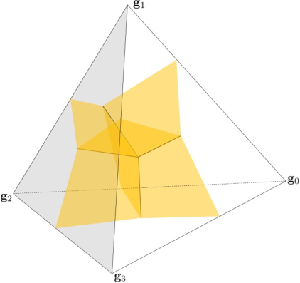
The phase produced by a Pachner move is expressed as a function $\omega:G^{5}\to\mathrm{U}(1)$ where $G^{5}$ denotes group elements on five 0-simplices on $S^{3}$ that characterizes a background gauge fields on $S^{3}$. $\omega$ turns out to take a value in a 4-cocycle $Z^{4}(BG,\mathrm{U}(1))$, and characterizes a ’t Hooft anomaly of the (2+1)D bulk [30]. Then, it has been shown in [29] that the ’t Hooft anomaly must be trivial when the bulk admits a symmetry-preserving gapped boundary, so we set $\omega=0$. It means that the bubble can be created without producing any phase.

Then, we eliminate the bubble by pushing it into the boundary. It involves a Pachner move on boundary, every time a codimension-3 junction of defects at the center of a 3-simplex gets absorbed in the boundary, see Fig. 4. We write the phase produced by a boundary Pachner move as $\alpha:G^{4}\to\mathrm{U}(1)$, as a function of group labels on the four vertices of a 3-simplex. The overall phase factor to eliminate the bubble is given by $\delta\alpha$ evaluated on a 4-simplex.

Since $\delta\alpha=0$ due to the vanishing of ’t Hooft anomaly in the bulk, $\alpha$ takes its value in $Z^{3}(BG,\mathrm{U}(1))$. When the gauge transformation on the boundary shifts the partition function by a phase $\alpha\in Z^{3}(BG,\mathrm{U}(1))$, one can cancel the phase ambiguity by coupling the bulk with a (2+1)D bosonic SPT phase characterized by the 3-cocycle $\alpha$. This process makes the bulk-boundary system gauge invariant without modifying the boundary condition, or the data of symmetry-enriched topological phase in the bulk (i.e., anyons and their symmetry fractionalization). Hence, one can assume without loss of generality that gauge transformations of flat background $G$ gauge field in the bulk-boundary system leave the partition function invariant.

Now, let us consider a junction of three symmetry defects $\mathbf{g},\mathbf{h},\mathbf{gh}\in G$ in the 3-manifold, then carve out a tube piercing the symmetry defects, as shown in Fig. 5. We introduce the gapped boundary condition on the boundary of the tube, where symmetry defects in 3D end on symmetry defects on the boundary theory.

Then, by performing background gauge transformation, one can move the junction of symmetry defects across the tube. By shrinking the tube during the process of the gauge transformations, one can see that symmetry fractionalization on the Lagrangian algebra anyon is trivial (see Appendix B for a review of symmetry fractionalization),

Also, consider cutting out the junction of three tubes and introducing the gapped boundary condition on its boundary, see Fig. 6. Then, by performing background gauge transformation across the junction, we obtain

which means that $G$ symmetry acts trivially on the fusion space $V^{\mathcal{L},\mathcal{L}}_{\mathcal{L}}$.

In particular, suppose that we can fix a gauge as $U_{\mathbf{g}}(a,b;c)=1$ for any $a,b,c\in\mathcal{C}$ with $N^{ab}_{c}>0$ and $\mathbf{g}\in G$, and consider a symmetry-preserving gapped boundary in this fixed gauge. We can then express symmetry fractionalization as $\eta_{a}(\mathbf{g},\mathbf{h})=M_{a,\mathfrak{t}(\mathbf{g},\mathbf{h})}$ using some Abelian anyon $\mathfrak{t}(\mathbf{g},\mathbf{h})\in\mathcal{C}$, which gives an element of $Z^{2}_{\rho}(BG,\mathcal{B})$ where $\mathcal{B}$ is a group of Abelian anyons in $\mathcal{C}$. Then, by using the property $SZ=Z$ of the Lagrangian algebra anyon we have

where $\mathcal{A}$ is the set of anyons with $Z_{0a}>0$. Since $S_{\mathfrak{t}(\mathbf{g},\mathbf{h}),b}=\frac{d_{b}M^{*}_{\mathfrak{t}(\mathbf{g},\mathbf{h}),b}}{\mathcal{D}}$ and $M_{b,\mathfrak{t}(\mathbf{g},\mathbf{h})}=\eta_{b}(\mathbf{g},\mathbf{h})=1$ when $b\in\mathcal{A}$, (2.8) is rewritten as

so we have $Z_{0,\mathfrak{t}(\mathbf{g},\mathbf{h})}>0$. Due to $TZ=Z$, we can see that $\mathfrak{t}(\mathbf{g},\mathbf{h})$ must be a boson, $\theta_{\mathfrak{t}(\mathbf{g},\mathbf{h})}=1$. More precisely, for a given symmetry fractionalization class $[\mathfrak{t}]\in H_{\rho}^{2}(BG,\mathcal{B})$, (2.6) should be understood as requiring the existence of natural isomorphism that picks a specific cocycle representative of $[\mathfrak{t}]$, so that $\eta_{a}(\mathbf{g},\mathbf{h})=1$ for $a\in\mathcal{A}$. The statement $\theta_{\mathfrak{t}(\mathbf{g},\mathbf{h})}=1$ is valid after performing such a natural isomorphism so that $\eta$ satisfies (2.6).

Here we comment on the simplicity of the Lagrangian algebra anyon in the presence of the global symmetry. Though a gapped boundary condition with $Z_{00}>1$ always decomposes into simple ones with $Z_{00}=1$ in the absence of the global symmetry, the symmetry-preserving boundary with $Z_{00}>0$ does not necessarily decompose into simple symmetric ones. In fact, for a given simple symmetry-breaking gapped boundary that violates (2.5), one can sum over the orbit of $G$ symmetry actions on it to obtain a $G$-symmetric boundary condition, which does not decompose into symmetry-preserving ones in general. However, when $G$ does not permute the anyons where (2.5) is satisfied, the constraints (2.6), (2.7) are obviously preserved for each decomposed component of the Lagrangian algebra anyons. Hence, we conjecture that the symmetric boundary condition with $Z_{00}>1$ always decomposes into simple symmetric ones with $Z_{00}=1$ when $[\rho]$ is trivial.

When $G=\mathrm{U}(1)$, the symmetry does not permute anyons. Symmetry fractionalization is then characterized by an assignment of fractional charge defined as follows. For a given set of $\{\eta,U\}$, one can define fractional charges of anyons that characterize the U(1) symmetry fractionalization as follows. For a fixed anyon $a$, let $n$ be the smallest integer such that $a^{n}$ contains the identity as a fusion product. Choose a sequence of anyons $a,a^{2},\dots a^{n}=1$ such that $a\times a^{k}$ contains $a^{k+1}$ as a fusion product. Then define a fractional charge $Q_{a}\in\mathbb{R}/\mathbb{Z}$ as [31]

where the elements of $\mathrm{U}(1)=\mathbb{R}/\mathbb{Z}$ is labeled by the numbers in $[0,1)$. One can check that the quantity $e^{2\pi iQ_{a}}$ is gauge-invariant. Since the map $[\rho]$ is trivial, we can fix a gauge where $U=1$, ²² 2 For modular tensor categories with the trivial symmetry action $[\rho]$, the existence of the gauge with $U=1$ is rigorously shown in Ref. [26] when all fusion coefficients satisfy $N^{c}_{a,b}\in\{0,1\}$. For the case with generic fusion coefficients, it is a conjecture given in Ref. [24]. so that $\eta$ satisfies ${\eta_{c}({\bf g},{\bf h})}=\eta_{a}({\bf g},{\bf h})\eta_{b}({\bf g},{\bf h})$ when $N^{c}_{ab}>0$. One can then see that

In the gauge where $U=1$, we can write the phases $\eta_{a}({\bf g},{\bf h})$ as

for Abelian anyon $\mathfrak{t}\in Z^{2}(B\mathrm{U}(1),\mathcal{B})$ where $\mathcal{B}$ is the set of Abelian anyons in $\mathcal{C}$. A representative 2-cocycle $\mathfrak{t}$ is given by $\mathfrak{t}({\bf g},{\bf h})=v^{{\bf g}+{\bf h}-[{\bf g}+{\bf h}]},$ where $v\in\mathcal{B}$ is referred to as the vison, $\mathbf{g},\mathbf{h}\in\mathbb{R}/\mathbb{Z}$ takes the values in $[0,1)$, and $[\mathbf{g}+\mathbf{h}]$ means the sum mod 1. Using the vison $v$, the fractional charge can be rewritten as [32]

Then, suppose that a bosonic TQFT with U(1) symmetry admits a U(1) symmetry-preserving gapped boundary, after setting the gauge $U=1$ by a suitable natural isomorphism. Then, (2.6) implies that

Hence, the vison $v$ has trivial mutual braiding with all $a\in\mathcal{A}$, $M_{a,v}=1$. Using the property of Lagrangian algebra anyon $SZ=Z$ and $S_{v,b}=\frac{d_{b}M^{*}_{v,b}}{\mathcal{D}}$, we obtain

so we have $Z_{0v}>0$. According to $TZ=Z$, we immediately see that the vison $v$ must be a boson, $\theta_{v}=1$.

As a straightforward application, we study an Abelian (2+1)D bosonic TQFT with U(1) symmetry. We prove the following statement:

Here, $N_{\mathrm{FS}}$ is the Frobenius-Schur exponent defined as the smallest positive integer such that $\theta_{a}^{N_{\mathrm{FS}}}=1$ for all $a\in\mathcal{C}$.

We provide a generic theory for topological gapped boundary of (2+1)D topological phases, which are effectively described by spin TQFT. For non-Abelian spin TQFTs, we make a generalization of Lagrangian algebra anyon for bosonic phases to fermionic cases, and express the gapped boundary condition of spin TQFT in algebraic form. In general, (2+1)D spin TQFT is described in terms of a super-modular tensor category $\mathcal{C}$ together with its minimal modular extension $\breve{\mathcal{C}}$. The basic description of spin TQFT are reviewed in Appendix C.

Let us assume that a spin TQFT has a gapped topological boundary condition. For a given 3-manifold, one can cut out a solid torus from it, and equip the resulting 3-manifold with a spin structure. We then introduce a gapped boundary condition on the boundary torus $T^{2}$. We can think of shrinking the radius of the tube of gapped boundary into a line, then the tube is eventually described by a line operator of spin TQFT. The expression of the line operator depends on the spin structure of the boundary torus $T^{2}$, and generally described by an object of a minimal modular extension $\breve{\mathcal{C}}$ of a super-modular tensor category $\mathcal{C}$.

We write spin structure on $T^{2}$ in the form of $T^{2}_{\mu,\lambda}$, where $\mu$ is spin structure on the meridian of the tube, and $\lambda$ is that on the longitude. We also write the minimal modular extension $\breve{\mathcal{C}}=\breve{\mathcal{C}}_{\mathrm{NS}}\oplus\breve{\mathcal{C}}_{\mathrm{R}}$ with $\breve{\mathcal{C}}_{\mathrm{NS}}=\mathcal{C}$ the NS sector.

To make an algebraic description of gapped boundary, it is convenient to consider a boundary state ${\left|{\mathcal{L}_{\mu,\lambda}}\right>}$ on a space $T^{2}_{\mu,\lambda}$ given by considering a spacetime $T^{2}_{\mu,\lambda}\times[0,1]$, and then introducing a gapped boundary condition on $T^{2}_{\mu,\lambda}\times\{1\}$. This defines a state ${\left|{\mathcal{L}_{\mu,\lambda}}\right>}$ on $T^{2}_{\mu,\lambda}\times\{0\}$. Equivalently, one can also regard the geometry as a solid torus $D^{2}\times S^{1}$, with a thin solid torus cut out at the center of $D^{2}$. So, the boundary state is thought of as an insertion of a line operator in $D^{2}\times S^{1}$ along $S^{1}$ obtained by a thin tube of gapped boundary.

Based on the description of Hilbert space for spin TQFT explained in Appendix C, the boundary state with each spin structure $(\mu,\lambda)$ is expressed as follows:

with $Z^{\mathrm{NS}}_{0[a]},Z^{\mathrm{R}}_{0[a]}$ set to be non-negative integers. The reasoning for the expression of the state is that spin structure along a closed curve is measured by inserting a Wilson line of the transparent fermion $\psi$ of $\mathcal{C}$ along the curve. For example, the $\psi$ line along the longitude acts by phase $+1$ (resp. $-1$) when spin structure along the longitude is NS (resp. R), hence the state is expressed in the form of ${\left|{a}\right>}+{\left|{a\times\psi}\right>}$ (resp. ${\left|{a}\right>}-{\left|{a\times\psi}\right>}$).

For simplicity, we assumed that the R sector $\breve{\mathcal{C}}_{\mathrm{R}}$ does not contain an anyon $\sigma$ with fusion rule $\sigma\times\psi=\sigma$ (which is called a “q-type” object). For example, when we are interested in spin TQFT with $\mathrm{U}(1)^{f}$ symmetry which is main interest in this paper, there exists no q-type object in $\breve{\mathcal{C}}_{\mathrm{R}}$ since the assignment of U(1) charge on anyons cannot be consistent with the fusion rule $\sigma\times\psi=\sigma$. So, this assumption does not lose generality in that case. The Hilbert space in the presence of q-type objects are illustrated in [36], and it would be interesting to study boundary conditions of such spin TQFTs.

The boundary states (3.1), (3.2) have several important properties under the $S,T$ transformation. Firstly, since the boundary is gapped and topological, the diffeomorphism acting on the gapped boundary at $T^{2}_{\mu,\lambda}\times\{1\}$ must not change the boundary state ${\left|{\mathcal{L}_{\mu,\lambda}}\right>}$. Since the torus is equipped with spin structure, the diffeomorphism here means the mapping class group of $T^{2}_{\mu,\lambda}$ leaving spin structure invariant.

For the case of $\mu=\mathrm{NS}$, the Dehn twist $T$ along the meridian exchanges the spin structure as $T^{2}_{\mathrm{NS},\mathrm{NS}}\leftrightarrow T^{2}_{\mathrm{NS},\mathrm{R}}$, so we have $T^{2}{\left|{\mathcal{L}_{\mathrm{NS},\mathrm{NS}}}\right>}={\left|{\mathcal{L}_{\mathrm{NS},\mathrm{NS}}}\right>}$. This implies that an anyon that appears in the summand of ${\left|{\mathcal{L}_{\mathrm{NS},\mathrm{NS}}}\right>}$ must be either a boson or a fermion, since Dehn twist acts on Wilson lines as ${\left|{a}\right>}\to\theta_{a}{\left|{a}\right>}$. For convenience, we write $\mathcal{A}_{\mathrm{NS}}=\mathcal{A}_{\mathrm{NS}}^{1}\sqcup\mathcal{A}_{\mathrm{NS}}^{\psi}$ as a set of anyons that appear in ${\left|{\mathcal{L}_{\mathrm{NS}}}\right>}$ (i.e., all $a,a\times\psi\in\breve{\mathcal{C}}_{\mathrm{NS}}$ with $Z_{0a}^{\mathrm{NS}}\neq 0$). $\mathcal{A}_{\mathrm{NS}}^{1}\subset\mathcal{A}_{\mathrm{NS}}$ is the set of bosons, and $\mathcal{A}_{\mathrm{NS}}^{\psi}\subset\mathcal{A}_{\mathrm{NS}}$ is the set of fermions. Note that $\mathcal{A}_{\mathrm{NS}}^{1}\cdot\psi=\mathcal{A}_{\mathrm{NS}}^{\psi}$.

Because of $T{\left|{\mathcal{L}_{\mathrm{NS},\mathrm{NS}}}\right>}={\left|{\mathcal{L}_{\mathrm{NS},\mathrm{R}}}\right>}$, the sum over a class of anyons $[a]=\{a,a\times\psi\}$ in (3.1) is fixed to be the sum over bosons $\mathcal{A}_{\mathrm{NS}}^{1}$. We then have

where we define $Z_{0a}^{\mathrm{NS}}=Z_{0,a\times\psi}^{\mathrm{NS}}=Z_{0[a]}^{\mathrm{NS}}$.

For the case of $\mu=\mathrm{R}$, the Dehn twist along the meridian leaves the spin structure invariant, so we have $T{\left|{\mathcal{L}_{\mathrm{R},*}}\right>}={\left|{\mathcal{L}_{\mathrm{R},*}}\right>}$. This means that an anyon that appears in the summand of ${\left|{\mathcal{L}_{\mathrm{R},*}}\right>}$ must be a boson. For convenience, we again write $\mathcal{A}_{\mathrm{R}}=\mathcal{A}_{\mathrm{R}}^{e}\sqcup\mathcal{A}_{\mathrm{R}}^{m}$ as a set of anyons that appear in ${\left|{\mathcal{L}_{\mathrm{R}}}\right>}$ (i.e., all $a,a\times\psi\in\breve{\mathcal{C}}_{\mathrm{R}}$ with $Z_{0a}^{\mathrm{R}}\neq 0$). The decomposition $\mathcal{A}_{\mathrm{R}}^{e}\sqcup\mathcal{A}_{\mathrm{R}}^{m}$ is taken to satisfy $\mathcal{A}_{\mathrm{R}}^{e}\times\psi=\mathcal{A}_{\mathrm{R}}^{m}$. We note that there is no canonical way to perform the decomposition into $\mathcal{A}_{\mathrm{R}}^{e}$ and $\mathcal{A}_{\mathrm{R}}^{m}$ unlike the case of NS sector, since all anyons of $\mathcal{A}_{\mathrm{R}}$ are bosons. We have

where we define $Z_{0a}^{\mathrm{R}}=Z_{0,a\times\psi}^{\mathrm{R}}=Z_{0[a]}^{\mathrm{R}}$.

Next, we discuss the property of the boundary states under the $S$ transformation. In the spacetime manifold $S^{3}$, let us consider a Hopf link between the thin tube of gapped boundary and a line operator $x$, as described in Fig. 8. This Hopf link can be evaluated in two ways. On one hand, the amplitude of the Hopf link is computed by the modular $S$-matrix of a modular category $\breve{\mathcal{C}}$ between two states on $T^{2}$, the boundary state ${\left|{\mathcal{L}}\right>}$ and ${\left|{x}\right>}$ respectively. On the other hand, one can enlarge the radius of the boundary tube, which makes the geometry $D^{2}\times S^{1}$ with the gapped boundary on $T^{2}$. It then reduces to a partition function on $D^{2}\times S^{1}$ with a $x$ line inserted along $S^{1}$. Comparing these two distinct expressions put a nontrivial constraint on the vectors $Z_{0a}$.

The analysis of $S$-matrix action on boundary states requires a lengthy discussion done by cases for spin structure of the spatial torus, and the detail is relegated to Appendix D. Here we summarize the $S$-matrix actions on $Z_{0a}$ obtained as follows:

(3.7) also holds when $a$ is not an element of $\mathcal{A}_{\mathrm{NS}}$, where both lhs and rhs becomes zero.

(3.8) also holds when $a$ is not an element of $\mathcal{A}_{\mathrm{R}}$, where both lhs and rhs becomes zero.

In the above study of the $S$-matrix action on boundary states, we obtained a bunch of equations in the form of $2SZ=\pm Z$ for each spin structure. We can express the above many equations in a much simpler way, with help of toric code $D(\mathbb{Z}_{2})$ with anyons $\{1,\psi,e,m\}$ and $S$-matrix $S^{\mathrm{tc}}$. The above properties of the boundary states under the action of $S$-matrix (3.5) (3.6) (3.7) (3.8) are then neatly summarized as

with $x,y\in D(\mathbb{Z}_{2})$. Then, let us define a new set of anyons $\widetilde{\mathcal{A}}_{\mathrm{NS}}\subset\breve{\mathcal{C}}_{\mathrm{NS}}\boxtimes D(\mathbb{Z}_{2})$ as

Here $\boxtimes$ denotes the Deligne product, which physically means stacking two independent theories.

We also define $\widetilde{\mathcal{A}}_{\mathrm{R}}\subset\breve{\mathcal{C}}_{\mathrm{R}}\boxtimes D(\mathbb{Z}_{2})$ as

We can then write the equations in terms of $S$-matrix of $\breve{\mathcal{C}}\boxtimes D(\mathbb{Z}_{2})$ as

Finally, by writing the combined vector $\widetilde{Z}:=Z_{\mathrm{NS}}\oplus Z_{\mathrm{R}}$ and $\widetilde{\mathcal{A}}:=\widetilde{\mathcal{A}}_{\mathrm{NS}}\sqcup\widetilde{\mathcal{A}}_{\mathrm{R}}$, we obtain

and it is not hard to see that the lhs becomes zero when $a$ is not an element of $\widetilde{\mathcal{A}}$. That is, the vector $\widetilde{Z}$ gives an eigenvector of the $S$-matrix of $\breve{\mathcal{C}}\boxtimes D(\mathbb{Z}_{2})$, $S\widetilde{Z}=\widetilde{Z}$. Since the anyons in $\widetilde{\mathcal{A}}$ are all bosons, we also have $T\widetilde{Z}=\widetilde{Z}$. So, a newly constructed object $\widetilde{\mathcal{L}}:=\sum_{a\in\widetilde{\mathcal{A}}}\widetilde{Z}_{0a}a$ satisfies the crucial property for the Lagrangian algebra anyon of a bosonic TQFT $\breve{\mathcal{C}}\boxtimes D(\mathbb{Z}_{2})$. Hence, we expect that $\widetilde{Z}$ describes a bosonic gapped boundary of a bosonic modular theory $\breve{\mathcal{C}}\boxtimes D(\mathbb{Z}_{2})$.

Physically, the gapped boundary of a fermionic theory $\mathcal{C}$ is regarded as a gapped interface between $\mathcal{C}$ and a trivial fermionic invertible phase. By gauging fermion parity $\mathbb{Z}_{2}^{f}$ of the whole system in the presence of the gapped boundary, we obtain a bosonic gapped interface between $\breve{\mathcal{C}}$ and a $\mathbb{Z}_{2}$ toric code $D(\mathbb{Z}_{2})$, where the toric code $D(\mathbb{Z}_{2})$ corresponds to gauging a trivial fermionic invertible phase. Since $D(\mathbb{Z}_{2})=\overline{D(\mathbb{Z}_{2})}$, it implies the existence of the gapped boundary for a bosonic theory $\breve{\mathcal{C}}\boxtimes D(\mathbb{Z}_{2})$. In the next subsection, we confirm this physical intuition by checking the other additional properties of Lagrangian algebra anyon.

References

- [1] D. C. Tsui, H. L. Stormer, and A. C. Gossard, “Two-dimensional magnetotransport in the extreme quantum limit,” Phys. Rev. Lett. 48 (1982) 1559.
- [2] R. B. Laughlin, “Anomalous quantum hall effect: An incompressible quantum fluid with fractionally charged excitations,” Phys. Rev. Lett. 50 (1983) 1395.
- [3] F. Wilczek, “Magnetic flux, angular momentum, and statistics,” Phys. Rev. Lett. 48 (Apr, 1982) 1144–1146. https://link.aps.org/doi/10.1103/PhysRevLett.48.1144.
- [4] G. Moore and N. Read, “Nonabelions in the fractional quantum hall effect,” Nuclear Physics B 360 no. 2-3, (1991) 362 – 396.
- [5] M. Banerjee, M. Heiblum, V. Umansky, D. E. Feldman, Y. Oreg, and A. Stern, “Observation of half-integer thermal hall conductance,” Nature 559 no. 7713, (Jun, 2018) 205–210.
- [6] A. Kitaev and L. Kong, “Models for Gapped Boundaries and Domain Walls,” Commun. Math. Phys. 313 no. 2, (2012) 351–373, arXiv:1104.5047 [cond-mat.str-el].
- [7] A. Kapustin and N. Saulina, “Topological boundary conditions in abelian Chern-Simons theory,” Nucl. Phys. B845 (2011) 393–435, arXiv:1008.0654 [hep-th].
- [8] A. Kapustin, “Ground-state degeneracy for abelian anyons in the presence of gapped boundaries,” Phys. Rev. B 89 no. 12, (2014) 125307, arXiv:1306.4254 [cond-mat.str-el].
- [9] M. Barkeshli, C.-M. Jian, and X.-L. Qi, “Classification of Topological Defects in Abelian Topological States,” Phys. Rev. B 88 (2013) 241103, arXiv:1304.7579 [cond-mat.str-el].
- [10] L.-Y. Hung and Y. Wan, “Ground State Degeneracy of Topological Phases on Open Surfaces,” Phys. Rev. Lett. 114 no. 7, (2015) 076401, arXiv:1408.0014 [cond-mat.str-el].
- [11] J. Wang and X.-G. Wen, “Boundary Degeneracy of Topological Order,” Phys. Rev. B 91 no. 12, (2015) 125124, arXiv:1212.4863 [cond-mat.str-el].
- [12] T. Lan, J. C. Wang, and X.-G. Wen, “Gapped Domain Walls, Gapped Boundaries and Topological Degeneracy,” Phys. Rev. Lett. 114 no. 7, (2015) 076402, arXiv:1408.6514 [cond-mat.str-el].
- [13] L. Kong and H. Zheng, “A mathematical theory of gapless edges of 2d topological orders. Part I,” JHEP 02 (2020) 150, arXiv:1905.04924 [cond-mat.str-el].
- [14] J. Kaidi, Z. Komargodski, K. Ohmori, S. Seifnashri, and S.-H. Shao, “Higher central charges and topological boundaries in 2+1-dimensional tqfts,” 2021. https://arxiv.org/abs/2107.13091.
- [15] A. Davydov, M. Müger, D. Nikshych, and V. Ostrik, “The witt group of non-degenerate braided fusion categories,” Journal für die reine und angewandte Mathematik (Crelles Journal) 2013 no. 677, (2013) 135–177.
- [16] J. Fuchs, C. Schweigert, and A. Valentino, “Bicategories for boundary conditions and for surface defects in 3-d TFT,” Commun. Math. Phys. 321 (2013) 543–575, arXiv:1203.4568 [hep-th].
- [17] A. Davydov, D. Nikshych, and V. Ostrik, “On the structure of the witt group of braided fusion categories,” Selecta Mathematica 19 no. 1, (2013) 237–269, arXiv:1109.5558.
- [18] F. A. Bais and J. K. Slingerland, “Condensate induced transitions between topologically ordered phases,” Phys. Rev. B 79 (2009) 045316, arXiv:0808.0627 [cond-mat.mes-hall].
- [19] F. J. Burnell, “Anyon condensation and its applications,” Ann. Rev. Condensed Matter Phys. 9 (2018) 307–327, arXiv:1706.04940 [cond-mat.str-el].
- [20] S.-H. Ng, A. Schopieray, and Y. Wang, “Higher gauss sums of modular categories,” Selecta Mathematica 25 no. 4, (Aug, 2019) , arXiv:1812.11234 [math.QA]. http://dx.doi.org/10.1007/s00029-019-0499-2.
- [21] S.-H. Ng, E. C. Rowell, Y. Wang, and Q. Zhang, “Higher central charges and witt groups,” 2020. https://arxiv.org/abs/2002.03570.
- [22] A. Kitaev, “Anyons in an exactly solved model and beyond,” Annals of Physics 321 (2006) 2–111, arXiv:cond-mat/0506438.
- [23] A. Kitaev, “Toward topological classification of phases with short-range entanglement,” 2011. https://online.kitp.ucsb.edu/online/topomat11/kitaev/.
- [24] M. Barkeshli, P. Bonderson, M. Cheng, and Z. Wang, “Symmetry fractionalization, defects, and gauging of topological phases,” Phys. Rev. B 100 (Sep, 2019) 115147, arXiv:1410.4540.
- [25] M. Lapa and M. Levin, “Anomaly indicators for topological orders with u(1) and time-reversal symmetry,” Physical Review B 100 no. 16, (Oct, 2019) , arXiv:1905.00435. http://dx.doi.org/10.1103/PhysRevB.100.165129.
- [26] F. Benini, C. Córdova, and P.-S. Hsin, “On 2-group global symmetries and their anomalies,” Journal of High Energy Physics 2019 no. 3, (Mar, 2019) 118, arXiv:1803.09336.
- [27] R. Kobayashi and M. Barkeshli, “(3+1)d path integral state sums on curved u(1) bundles and u(1) anomalies of (2+1)d topological phases,” 2021. https://arxiv.org/abs/2111.14827.
- [28] N. Seiberg and E. Witten, “Gapped boundary phases of topological insulators via weak coupling,” Progress of Theoretical and Experimental Physics 2016 no. 12, (2016) 1–86, arXiv:1602.04251v3.
- [29] R. Thorngren and Y. Wang, “Anomalous symmetries end at the boundary,” Journal of High Energy Physics no. 9, (2021) 17, arXiv:2012.15861.
- [30] X. Chen, Z.-C. Gu, Z.-X. Liu, and X.-G. Wen, “Symmetry-protected topological orders in interacting bosonic systems,” Science 338 no. 6114, (2012) 1604–1606, http://www.sciencemag.org/content/338/6114/1604.full.pdf.
- [31] D. Bulmash and M. Barkeshli, “Fermionic symmetry fractionalization in (2+1)d,” 2021. https://arxiv.org/abs/2109.10913.
- [32] M. Cheng, M. Zaletel, M. Barkeshli, A. Vishwanath, and P. Bonderson, “Translational symmetry and microscopic constraints on symmetry-enriched topological phases: A view from the surface,” Phys. Rev. X 6 (Dec, 2016) 041068, arXiv:1511.02263. https://link.aps.org/doi/10.1103/PhysRevX.6.041068.
- [33] N. Reshetikhin and V. G. Turaev, “Invariants of 3-manifolds via link polynomials and quantum groups,” Inventiones mathematicae 103 no. 1, (1991) 547–597. https://doi.org/10.1007/BF01239527.
- [34] V. G. Turaev, Quantum Invariants of Knots and 3-Manifolds. De Gruyter, 2010. https://doi.org/10.1515/9783110221848.
- [35] V. Drinfeld, S. Gelaki, D. Nikshych, and V. Ostrik, “On braided fusion categories i,” 2010. https://arxiv.org/abs/0906.0620.
- [36] D. Delmastro, D. Gaiotto, and J. Gomis, “Global anomalies on the hilbert space,” 2021. http://arxiv.org/abs/2101.02218.
- [37] D. Aasen, P. Bonderson, and C. Knapp, “Characterization and classification of fermionic symmetry enriched topological phases,” 2021. https://arxiv.org/abs/2109.10911.
- [38] Z.-C. Gu and X.-G. Wen, “Symmetry-protected topological orders for interacting fermions: Fermionic topological nonlinear models and a special group supercohomology theory,” Phys. Rev. B 90 (Sep, 2014) 115141, arXiv:1201.2648. https://link.aps.org/doi/10.1103/PhysRevB.90.115141.
- [39] A. Kapustin, R. Thorngren, A. Turzillo, and Z. Wang, “Fermionic Symmetry Protected Topological Phases and Cobordisms,” JHEP 12 (2015) 052, arXiv:1406.7329 [cond-mat.str-el].
- [40] Q.-R. Wang and Z.-C. Gu, “Construction and classification of symmetry protected topological phases in interacting fermion systems,” Physical Review X 10 (2018) 031055, arXiv:1811.00536.
- [41] R. Thorngren, “Anomalies and bosonization,” arXiv:1810.04414. https://arxiv.org/abs/1810.04414.
- [42] M. Barkeshli, Y.-A. Chen, P.-S. Hsin, and N. Manjunath, “Classification of (2+1)d invertible fermionic topological phases with symmetry,” 2021. https://arxiv.org/abs/2109.11039.
- [43] L. Bhardwaj, D. Gaiotto, and A. Kapustin, “State sum constructions of spin-tfts and string net constructions of fermionic phases of matter,” Journal of High Energy Physics 2017 no. 96, (2017) . https://doi.org/10.1007/JHEP04(2017)096.
- [44] Y. Wan and C. Wang, “Fermion condensation and gapped domain walls in topological orders,” Journal of High Energy Physics 2017 no. 3, (Mar, 2017) , arXiv:1607.01388 [cond-mat.str-el]. http://dx.doi.org/10.1007/JHEP03(2017)172.
- [45] C. Heinrich and M. Levin, “Criteria for protected edge modes with symmetry,” Physical Review B 98 no. 3, (Jul, 2018) , arXiv:1803.00023 [cond-mat].
- [46] T.-J. Freyd and D. Reutter, “Minimal nondegenerate extensions,” 2021. https://arxiv.org/abs/2105.15167.
- [47] P. Bruillard, C. Galindo, T. Hagge, S.-H. Ng, J. Y. Plavnik, E. C. Rowell, and Z. Wang, “Fermionic modular categories and the 16-fold way,” Journal of Mathematical Physics 58 no. 4, (Apr, 2017) 041704, arXiv:1603.09294. http://dx.doi.org/10.1063/1.4982048.
- [48] Y. Tachikawa, “On gauging finite subgroups,” SciPost Phys. 8 no. 1, (2020) 015, arXiv:1712.09542 [hep-th].
- [49] S. Tata, R. Kobayashi, D. Bulmash, and M. Barkeshli, “Anomalies in (2+1)d fermionic topological phases and (3+1)d path integral state sums for fermionic spts,” 2021. https://arxiv.org/abs/2104.14567.
- [50] R. Thorngren, “Framed wilson operators, fermionic strings, and gravitational anomaly in 4d,” Journal of High Energy Physics 2015 no. 2, (Feb, 2015) . http://dx.doi.org/10.1007/JHEP02(2015)152.
- [51] D. Gaiotto and A. Kapustin, “Spin TQFTs and Fermionic Phases of Matter,” Int. J. Mod. Phys. A31 no. 28n29, (2016) 1645044, arXiv:1505.05856 [cond-mat.str-el].
- [52] D. Aasen, E. Lake, and K. Walker, “Fermion condensation and super pivotal categories,” Journal of Mathematical Physics 60 no. 12, (Dec, 2019) 121901, arXiv:1709.01941. http://dx.doi.org/10.1063/1.5045669.
- [53] Karlheinz Knapp, “Wu class.” http://www.map.mpim-bonn.mpg.de/Wu_class.
- [54] S. Tata, “Geometrically interpreting higher cup products, and application to combinatorial pin structures,” 2020. https://arxiv.org/abs/2008.10170.