Implicit Feature Decoupling with Depthwise Quantization
Abstract
Quantization has been applied to multiple domains in Deep Neural Networks (DNNs). We propose Depthwise Quantization (DQ) where quantization is applied to a decomposed sub-tensor along the feature axis of weak statistical dependence. The feature decomposition leads to an exponential increase in representation capacity with a linear increase in memory and parameter cost. In addition, DQ can be directly applied to existing encoder-decoder frameworks without modification of the DNN architecture. We use DQ in the context of Hierarchical Auto-Encoders and train end-to-end on an image feature representation. We provide an analysis of the cross-correlation between spatial and channel features and propose a decomposition of the image feature representation along the channel axis. The improved performance of the depthwise operator is due to the increased representation capacity from implicit feature decoupling. We evaluate DQ on the likelihood estimation task, where it outperforms the previous state-of-the-art on CIFAR-10, ImageNet-32 and ImageNet-64. We progressively train with increasing image size a single hierarchical model that uses 69% fewer parameters and has faster convergence than the previous work.
1 Introduction


Quantization is an effective lossy compression process that maps a continuous signal to a set of discrete values, also called codes. Quantization is extended to vector feature spaces with learning paradigms such as Vector Quantization (VQ) and with a training objective identical to k-means. Product Quantization (PQ) decomposes the feature vector and assumes a weak statistical dependence between feature sub-vectors. Additive Quantization (AQ) decomposes the feature vector into a sum of quantized vectors as opposed to the concatenated output in PQ.

Quantization is used in conjunction with Deep Neural Networks (DNNs) for tasks such as classificationprototype_cnn, incremental learningprototype_cnn, zero-shot learning zero_shot_prototype, generation vqvae, compression image_compression and data retrieval cao_image_retrieval. The discrete quantized feature representations can be used post-hoc vqvae; vqvae2; jukebox or as a learning objective (i.e. classification) zero_shot_prototype; prototype_cnn. Our work is motivated by the increasing number of quantization applications to high dimensional feature tensors. We view the quantizer as a density estimator and evaluate it on the task of likelihood estimation for the visual domain.
Likelihood estimation models seek to minimize the divergence between the data distribution and the model prior. Explicit likelihood estimation models, including Vector Quantization (VQ), Variational Auto-encoders (VAEs), and Auto-Regressive (AR) models directly minimize a divergence. In this work, we focus on explicit likelihood estimation.
AR models do well in likelihood estimation and are applied in multiple domains such as language, vision, and audio. AR models have a recursive dependency on the input during training and inference. Therefore, AR models are computationally inefficient for domains with long sequences, such as pixels of an image. Even with caching cache_wavenet during sampling, AR models are still less efficient than VAEs.
The priors of VAEs provide a compressed feature representation that can be used as a surrogate training objective for the downstream task. In contrast to the discrete prior, a continuous prior can lead to posterior collapse. The representation is ignored by the downstream task model because it is either too noisy or uninformative. This effect is amplified when the data is discrete, as in the language domainz_forcing.
To that end, we propose the Depthwise Quantization (DQ) method that quantizes each decomposed feature sub-tensor with a different quantizer. We use rate-distortion theory to interpret a quantizer as an encoding function with limited capacity. We provide a theoretical upper bound on the capacity in relation to the quantization cost when DQ is applied on a decoupled feature tensor, as opposed to a coupled feature tensor. We evaluate the performance of DQ on the feature space of ImageNet for an image classification backbone. Lastly, we apply DQ to a hierarchical Auto-Encoder with DQ as a bottleneck for different hierarchies and train it end-to-end. DQ outperforms explicit models in likelihood estimation. In detail:
- •
We propose Depthwise Quantization (DQ) and decompose a feature tensor along the axis of weak statistical dependence.
- •
We provide a theoretical analysis on the improved quantization performance and experimentally corroborate our theoretical results.
- •
We introduce an improved hierarchical AutoEncoder model Depth-Quantized Auto-Encoder where DQ is applied to the feature representation at different hierarchies.
- •
We extend the parametric Mutual Information (MI) quantization estimators for DNNs when the prior is learned. We experimentally verify that the learned prior is implicitly decoupled.
Our approach can be applied to previous works that use quantization. We demonstrate with our experiments that DQ performs significantly better when the assumption on cross-correlation is strong in both post-hoc analysis and end-to-end training settings. When trained end-to-end, DQ reduces the cross-correlation among the decomposed feature tensors (‘‘implicitly decouple’’) and improves reconstruction loss and likelihood estimation. Our code is publicly available11 1 https://github.com/fostiropoulos/Depthwise-Quantization.
2 Related Work
Our work is closely related to previous studies on feature decomposition and quantization optimization in visual tasks using DNNs.
Feature decomposition approaches include Separable Convolutions (SP) seperable_convnets, which factorizes a convolutional kernel to the spatial dimensions. SP reduces the number of computations required to calculate the filter output. Inception inception, another approach to feature decomposition, factorizes a feature representation implicitly with a “Network-in-Network” (NiN) network_in_network branch of convolutions. Thus, Inception learns spatial cross-correlations and feature cross-correlations independently. Depthwise Separable Convolution (DSC) xception; inception is a method of feature decomposition that uses a single “spatial” convolution followed by multiple vanilla convolutions on a decomposed “segment”. Xceptionxception is based on the “Inception Hypothesis” for a decoupled space where DSC is applied to an eXtreme. Our work is based on a hypothesis similar to that of DSC and considers modeling cross-channel correlations and spatial correlations independently.
There are analyses on the decoupling of the feature space implicitly in the context of DSC as well as on NiN architectures. Blueprint Separable Convolutions (BSConv) bsconv have been proposed as an alternative to DSC based on the observation of intra-kernel correlations. They propose a pointwise (1x1) convolution followed by a depthwise convolution. In contrast, DSC enforces cross-kernel correlations implicitly. Analysis on the variance of a convolution kernel shows that a DNN can perform better when cross-kernel redundancies decrease.
Other works explicitly factorize a convolutional filter. There are methods that use a low-rank approximation low_rank_aprox_conv or closed-form decomposition network_decoupling on pre-trained networks to speed up the computation process. Previous works on speeding up networks quantization_kernel have used product quantization to quantize convolutional filters and take advantage of the redundancies. Previous analysis of the redundancy and cross-correlation of the feature space in DNNs is complementary to our work.
Improvements in quantization learning approaches include Optimized Product Quantization optimized_pq that decomposes the feature vector in a parametric manner. In addition, Additive Quantization additive_quantization improves on the computational efficiency of PQ for high dimensional vector search by decomposing the vectors into a sum instead of a concatenation of their sub-vectors. In contrast, our work can be applied to feature tensors and the quantizer is trained end-to-end with a DNN.
Kobayashi et al. decomposing_medical_images train a quantizer end-to-end with a DNN. They use multiple codebooks and train each codebook independently for a different supervised task. However, as opposed to our method, the codebooks are decoupled in a supervised manner. Moreover, the quantized representations are used by different networks for different downstream tasks as opposed to interacting for a single downstream task. Lastly, vector decomposition is applied to feature vectors as opposed to feature sub-tensors as in our work.
PQ-VAE pqvae also decomposes the latent representations to sub-vectors and uses different quantizers for each sub-vector. Kaiser et al. fast_decoding introduces “sliced quantization” that is identical to PQ-VAE but uses the discrete representation post-hoc with a latent variable model. By contrast, DQ decomposes the feature space to sub-tensors as opposed to sub-vectors and thus improves the reconstruction loss by implicitly increasing the statistical dependence within the sub-tensor.
The works most similar to ours are those of Razavi et al. vqvae2 and Dhariwal et al. jukebox. VQ-VAE-2 vqvae2 applies quantization to the feature representation of multiple hierarchies on a VAE. Similar to our method, they train VQ end-to-end with a VAE. However, we apply DQ as opposed to VQ for the quantization method. VQ-VAE-2 can suffer from an uninformative top prior. Subsequent models such as “Jukebox” jukebox mitigate the issue by modeling each hierarchy with an independent encoder-decoder architecture. We also avoid the issue of an uninformative top prior but do not model each hierarchy with a different model. Instead, we introduce a model architecture DQ-AE.
3 Background


Auto-Encoder (AE) is an unsupervised class of DNN architectures that learns compressed feature representations from high dimensional data. Work by Kingma et al. vae extends AE to Deep Latent Variable Models with variants such as Variational Auto-Encoder (VAE). For some input and a latent space , VAE is composed of a decoder , a prior , and an encoder . VAE is a probabilistic model that implicitly learns underlying variables used to generate the data and their latent factors by minimizing the divergence between the encoded representation and the true data manifold . To evaluate AE, we can use Mutual Information (MI) which is a statistical dependence metric between two variables s.t. , where is the information entropy of . The optimization objective of a VAE beta-vae; beta_understanding is an upper bound to
| (1) |
that maximizes the mutual information between latent representation and decoded data, and discards information from x that is not informative to decoding . As such, maximizing Eq. 1 also maximizes the entropy of or “informativeness” hutter2002distribution.
Our view on quantization is based on the interpretation by Richardson et al. richardson2008modern and MacKay et al. mackay2003information. For the sake of brevity, we refer the reader to their work for a detailed analysis and attach our own analysis and proofs in the supplementary material.
Scalar Quantizer (SQ) with a vocabulary of size is an encoding function for an element from a sequence of length such that . SQ quantizes every element of the sequence in a memory-less fashion with the same encoding function. SQ cannot place assumptions on cross-correlation between different sequence elements. SQ performs optimally when the probability density function (pdf) of all data is known in advance. An encoding function that follows a uniform distribution (i.e. floor function) will perform optimally when all are also uniformly distributed and bounded such that . When has an unknown pdf, SQ will assign probability mass on unlikely regions in .
Vector Quantization (VQ) “learns” a mapping between , and quantization vectors, or codes. A Codebook is the set of codes such that . The VQ decoding function returns the code with the lowest decoding error between and the vector such that where . The objective function is to minimize the error of the closest codebook vector to the feature vector and can be summarized as .

Product Quantization (PQ) decomposes a one dimensional vector to sub-vectors and optimizes for a unique pair of a VQ and the sub-vector space. For different Codebooks there is a one-to-one mapping with each . The PQ decoding function is the concatenation or addition of all VQ decoding for codebook such that . We adopt the feature decomposition from PQ and extend it to high dimensional feature vectors to reduce the statistical independence among latent features.
Cost of a quantizer is the number of Codebook vectors s.t. , for PQ. Representation Capacity () defines an upper bound on the sample space from the number of discrete latent factors that can be represented by the quantizer for independent random variables , such that for codes and decomposed sub-vectors. For redundant , the sample space is reduced to and thus the capacity is bounded by the sample space s.t.
| (2) |
Note that for PQ, grows linearly while grows exponentially, in contrast to a VQ which has linear growth for both, and thus has an exponential cost with an identical capacity to PQ. More detailed analysis and proofs can be found in the Appendix.
Distribution of Prior can have an effect on the decoding performance of the quantizer. For example, VQ with from before can achieve identical decoding error as SQ but at a significant cost of as compared to for a memory-less SQ. The assumption on the distribution of the prior can determine the cost and the representation capacity of a quantizer.
The difference between PQ and VQ is the assumption of co-variance among features. Contrary to VQ, PQ takes advantage of the low co-variance among feature sub-vectors.
4 Depthwise Quantization
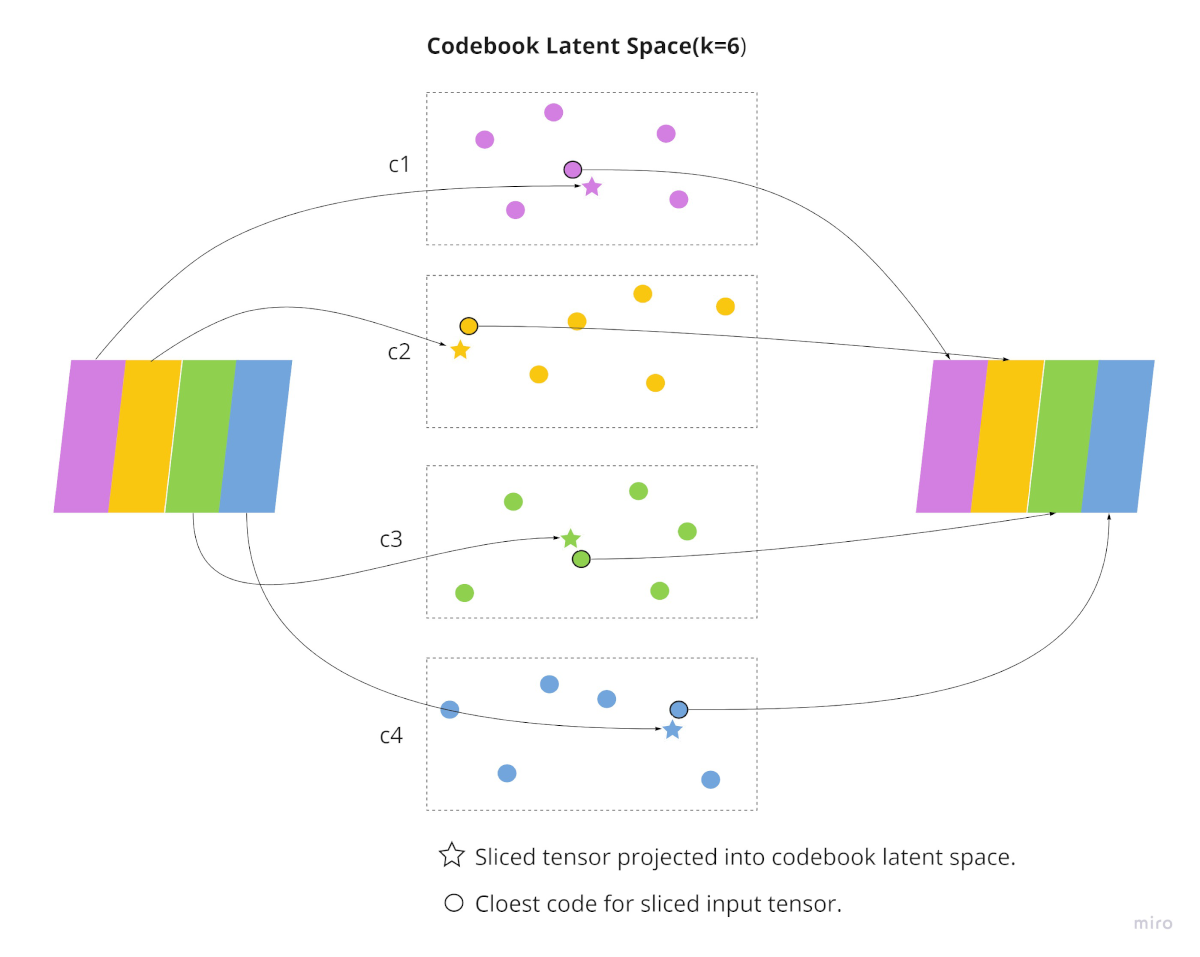
Given an output feature tensor from encoder with rank , Depthwise Quantization (DQ) applies quantizers pair-wise on decomposed tensor slices along an axis with quantization dimension .
| (3) |
Each optimizes Codebook and uses to define the error between and closest quantization vector . The optimization objective is the joint optimization over each codebook such that
| (4) |
We use the norm as a similarity metric for between each and the local quantization vector . The DQ loss is then added to the reconstruction loss of the DNN and the gradients are copied from the quantized vector to using auto-grad stop_grad. The loss function of DQ becomes
| (5) |
where stands for stop-gradient operator that stops the operand from updating during the training phase. Similar to the setting in VQ-VAE, the first loss term is used to lower the reconstruction error, the second term adjusts the codebook corresponding to the encoder output, and the third term is used to prevent the output of the encoder from growing arbitrarily. Note that the KL divergence is a constant equal to as DQ assumes a uniform prior distribution of latent embeddings. Therefore, the KL divergence term is dropped from the optimization objective of our framework. A detailed explanation is provided in Section 4.1
Note that for a feature tensor of rank one, DQ is identical to SQ when a single codebook of dimensionality one is used. When more than one codebook is used, DQ is identical to PQ and Additive Quantization with addition as the decoding function. The advantage of DQ over other quantization methods comes from the decomposition of a tensor to sub-tensors along the axis of weak statistical dependence.
For 2-D Convolutional Neural Networks (CNN), X is a feature tensor of rank 3. Fig. 2 provides an illustration of the DQ process for a 3-rank tensor. Different quantizers are applied for each slice of the channel axis, but the same quantizer is applied on the sub-vectors of a feature sub-tensor, such as decomposing along the spatial dimension.
4.1 Decoupled Feature Space
Decoupled refers to the statistical independence between features and Coupled refers to the statistical dependence between features. We use Information Theory to analyze quantization as an encoding function with an information bottleneck on a signal.
Eq. 1 provides the basis of the VAE optimization objective that can be formulated as a lower bound to the channel capacity as beta-vae; beta_understanding where is the Lagrange multiplier. -VAE assumes a Gaussian prior , and DQ assumes a uniform prior. Thus the KL-Divergence of the uniform distribution and decoder is the capacity of the quantizer . The detailed proof can be found in Appendix 1.
| (6) |
Reducing the capacity of the information bottleneck in VAE encourages disentangled representations in -VAE. In a similar fashion, reducing encourages disentangled representations for each codebook, with the upper bound controlled by and . By doing so, significantly compressed representations can be learned for an improved downstream training objective.
and by extension in the discrete case are not differentiable with respect to the DNN parameters and can not be explicitly minimized. We observe index collapse and performance degradation on hierarchical deep quantization variants. Index collapse causes the quantizer to utilize only limited number of codes. We enforce a uniform prior through an approximate solution and discuss the implications in Section 4.2 and Section 6.


4.2 Implicit Decoupling
Implicit decoupling of the feature space is the surrogate optimization objective derived by the explicit minimization of the decoding error. There is a joint optimization objective when DQ is applied to the intermediate feature representations in the context of DNN and trained end-to-end. DQ minimizes the decoding error along the DNN objective function. DQ works as a bottleneck on intermediate feature representations between subsequent layers of the network. We use the result from work by -VAE on the interpretation of AE as the information bottleneck.
-VAE uses to learn a set of additive channels where their capacity is maximized when all are independent. This provides an implicit optimization objective by optimizing Eq. 1, which is the equivalent in the quantized case as optimizing Eq. 6. There is an equivalence between each and the codebook as they both perform as additive information channels that, when combined, reconstruct an original signal. Lastly, both and the quantizer are parametric density estimators or smaller networks that can be considered as part of a generic Network-in-Network (NiN) family of models.
Feature independence improves downstream task performance when learned implicitly in NiN models. Xception uses Depthwise Seperable Convolution (DSC) to outperform coupled variants on ablation studies on Mobile-Net intra_kernel_cor. Additional previous analysis on the intra-kernel correlations bsconv has demonstrated the benefits of a decoupled feature space along the channels of an image feature tensor. We corroborate the analysis with MI estimation on a static prior to determine the axis of weak statistical dependence and apply DQ along the channel dimension (“depth-wise”) and spatial dimension (“pixel-wise”) in the context of DNN.
Uniform Prior In contrast to the traditional Variational Auto-Encoder, DQ relies on the assumption of uniform distribution of quantized vectors . However, the assumption of a uniform prior is not strong, which can potentially lead to degrading performance and be sensitive to the random initialization. A non-uniform prior will cause codebook collapse where only few codes are utilized in a codebook. To mitigate this issue, we follow previous work, and use Exponential Moving Average (EMA) and random re-initialization of codes. We re-initialize codes with low usage frequency counts that are below a threshold.Although previous works fast_decoding; on_line_em discuss the equivalence of quantization with EMA and the -VAE objective, there is no exact relationship between the two. VQ-VAE is an approximation to the Varitional Information Bottleneck (VIB) when trained with soft Expectation Maximization (EM). The E-step on the update rule of DQ is approximated with EMA over mini-batches of data on_line_em; chen2018stochastic. This is in contrast to hard - EM where quantization is deterministic roy2018theory. Soft - EM provides a probabilistic discrete information bottleneck as discussed in work by Roy et al. roy2018towards and Wu et al. wu2018variational.
We use entropy of the quantization vectors to measure their information density. A successful decoupling method should generate feature vectors with high entropy. Entropy Estimation on continuous distributions is intractable, but a signal can be discretized by quantization with both parametric and non-parametric optimization on the quantization interval. The entropy is then computed on the quantized discrete distribution.
| (7) |
We use the quantization regions of VQ as a density estimator for entropy, and thus mutual information on a continuous prior. When DQ is learned end-to-end, entropy can be calculated directly by the frequency count of each code vector over a sample set. Our approach in approximating MI is similar to previous work that uses Kernel Density Estimators kernel_density_estimator and is performed post-hoc on a trained network or by training a different DQ. Quantization post-hoc is sensitive to sample size but performs at par with other state-of-the-art approaches k-means-mi; k-means-mi-2; MI_estimation; paninski2003estimation.
4.3 Depth-Quantized AutoEncoder
Depthwise Quantized Auto-Encoder (DQ-AE) uses DQ at different hierarchical feature representations. The full algorithm that defines the training process is found in the supplementary material. In summary, we decode each quantized representation conditioned only on the quantized representation of the previous level. We perform this operation top-bottom and use Eq. 6 as the optimization objective of each DQ. Through experiments, we find that lower capacity bottom-level hierarchy enforces the utilization of top-level hierarchies and that the problem of under-utilization of top or bottom level hierarchies can also be a consequence of over-fitting. During the early stages of training, both hierarchies are used equivalently, but at later stages, top-level prior collapse. Our architecture leads to informative top and bottom level hierarchies as can be seen in Fig. 4.
5 Experiment
| CIFAR-10 | ImageNet-32 | ImageNet-64 | |||
|---|---|---|---|---|---|
| Model (Param.) | bits/dim | Param. | bits/dim | Param. | bits/dim |
| S-Tr.1 (59M) | 2.80 | Img-Tr.2 (-) | 3.77 | S-Tr.1 (152M) | 3.44 |
| VDVAE3 (39M) | 2.80 | 119M | 3.80 | 125M | 3.52 |
| (Ours) (22M) | 2.52 | 22M | 3.12 | 22M | 2.89 |
In our experiment, we evaluate DQ in two settings: on a static prior, and when trained end-to-end with a DNN, on a learned prior. We first evaluate our theoretical claim on a static prior and perform an ablation study on DQ and DQ-AE. We report the details of the training and network hyper-parameters in the supplementary material.
5.1 Density Estimation
We experimentally verify our claims on the decoupled feature space from Section 4.1. The penultimate feature representation from pre-trained VGG-16 model22 2 https://pytorch.org/vision/stable/models.html is used on ImageNet deng2009imagenet. DQ decomposes the feature representation “channel-wise” () and “pixel-wise” (). The penultimate feature tensor with shape is sliced along the channel axis into 7 segments and zero padded with and . The quantizers for both networks independently quantize each row for in contrast to each slice for .
We train DQ as a quantizer for multiple random runs (10) and we report the mean norm between X and the reconstruction . For each quantization method, we approximate the entropy of the codes to determine their respective information density using Eq. 7. The results of our experiments can be found in Table 2.
We find that DQ can achieve better density estimation along the channel dimension as opposed to the spatial dimension. The lower entropy of the feature tensor is due to a higher redundancy among feature sub-tensor and corresponds to a higher reconstruction error. DQ can perform better when decomposing on the channel axis and our results agree with previous analyses on intra-kernel correlations bsconv.
| Quant. | K | D | ||
|---|---|---|---|---|
| Pixel | 32 | 74 | 0.192 | 1.98 |
| Channel | 32 | 74 | 0.184 | 2.53 |
| Pixel | 1024 | 74 | 0.523 | 3.64 |
| Channel | 1024 | 74 | 0.480 | 3.99 |
5.2 Implicit Decoupling
We train a DQ-AE and a VQ-VAE vqvae for and with an identical network configuration, methodology and hyper-parameters. The difference between architectures is highlighted in Fig. 2. We measure the likelihood estimation of the two approaches on CIFAR-10krizhevsky2009learning and quantize each image to codes. VQ-VAE NLL is 4.36 bits/dim as compared to 3.14 bits/dim for single hierarchy DQ-AE, a 28% decrease.
High Entropy We show that the learned features of DQ have high entropy which indicates low statistical dependence among them. In contrast, VQ appears to have few very informative features and many uninformative ones. The mean entropy of the prior is nats/pixel for DQ as compared to nats/pixel for VQ. The entropy distribution among spatial features of the prior can be found in the left two sub-figures in Fig. 3.
Low MI We estimate the pairwise MI of the quantization vectors along the depth of the feature tensor with mean score of and nats/vector respectively. A comparison matrix can be found in the right two sub-figures in Fig. 3. For DQ the MI between quantization vectors is significantly lower as visualized by the mostly empty upper triangular matrix. In contrast, for VQ there seems to be higher redundancy among quantization vectors. The diagonal of the matrix represents the entropy of each quantization vector. The MI estimate on the quantization vector shows that the redundancies are significantly higher in the learned representation for VQ.
5.3 Ablation study
We study the effect of and on the model performance. The model is more sensitive to the dimensionality of the sub-vector and less sensitive to . DQ outperforms coupled variants on likelihood estimation and reconstruction loss in all settings. grows exponentially with as opposed to . Fewer code vectors can be used to quantize without performance degradation. For example, when , DQ outperforms a VQ variant by 35% and uses 25% fewer code vectors. Fig. 5 shows a summary of the loss for different and values. A detailed table of the results can be found in the Appendix.
5.4 Likelihood Estimation
For likelihood estimation, we compare DQ-AE with other likelihood estimator models and report the numbers from their work. We use Very Deep VAE (“VD-VAE”) vdvae as a continuous AutoEncoder baseline and Sparse Transformer (“S-Tr”) child2019generating as an Auto-Regressive baseline.
For experiments on ImageNet, we add a number on the image resolution at which we train the model at the end of the dataset name. For our model, we use an identical architecture and number of hierarchies for all resolution of the dataset. The detailed results are in Table 1. We outperform all previous state-of-the-art models when measuring the loss in bits/dim, we also report separately. The estimate for nats. Visual inspection of both top and bottom hierarchies confirm that they encode different granularity of features and are utilized (Fig. 4), and perceptual quality is improved (Fig. 1). Additional high resolution images are attached in the supplementary materials.
When compared to the hierarchical model by Razavi et al. vqvae2, DQ-AE also outperforms in reconstruction error for on ImageNet-256. On CIFAR-10, the DQ-AE loss is compared to for VQ-VAE. For ImageNet-256, DQ-AE loss is compared to for VQ-VAE-2.
6 Discussion
We thoroughly evaluate the theoretical claims of our work and empirically verify our method in likelihood estimation. Evaluation of the discrete representation on a downstream task such as latent interpolations is domain specific. Sampling from the multi-resolution and high dimensional discrete codebooks requires training additional models post-hoc. As such, there are multiple open problems in how to design such a model. We leave this for future work.
The direct evaluation and comparison on NLL between explicit likelihood models can be non-equivalent. Our model makes different assumptions on the prior distribution and as such the direct comparison can be flawed. Previous work alemi2018fixing has suggested that the ELBO might be a poor metric to evaluate deep latent variable models. We mitigated the issue and followed the theoretical result and experimental methodology to previous work vdvae. We consider the proper evaluation of the discrete prior with other model variants as an open problem.
7 Conclusion
We analyze the effects of decomposing an image feature tensor along an axis of statistical independence. Decomposition and quantization among independent features outperforms coupled feature variants. Our theoretical insights focus on feature decoupling for decomposed image feature tensors along the channel axis. Our results corroborate previous analyses and explain the advantage of NiN applications which can be interpreted as an information bottleneck.
Based on our theoretical insight, we propose Depthwise Quantization (DQ) that provides significantly more efficient bottleneck capacity by eliminating redundancies implicitly in the feature axis. DQ is trained end-to-end with a Hierarchical Auto-Encoder (DQ-AE) and learns improved hierarchical discrete representations. Our method is domain agnostic, and we consider the evaluation on a specific task for future work.
References
- (1) Alexander Alemi, Ben Poole, Ian Fischer, Joshua Dillon, Rif A Saurous, and Kevin Murphy. Fixing a broken elbo. In International Conference on Machine Learning, pages 159–168. PMLR, 2018.
- (2) Artem Babenko and Victor Lempitsky. Additive quantization for extreme vector compression. In Proceedings of the IEEE Conference on Computer Vision and Pattern Recognition, pages 931–938, 2014.
- (3) Christopher P Burgess, Irina Higgins, Arka Pal, Loic Matthey, Nick Watters, Guillaume Desjardins, and Alexander Lerchner. Understanding disentangling in -vae. arXiv preprint arXiv:1804.03599, 2018.
- (4) Yue Cao, Mingsheng Long, Jianmin Wang, and Shichen Liu. Deep visual-semantic quantization for efficient image retrieval. In Proceedings of the IEEE Conference on Computer Vision and Pattern Recognition, pages 1328–1337, 2017.
- (5) Olivier Cappé and Eric Moulines. On-line expectation-maximization algorithm for latent data models. Journal of the Royal Statistical Society: Series B (Statistical Methodology), 71(3):593–613, Jun 2009.
- (6) Jianfei Chen, Jun Zhu, Yee Whye Teh, and Tong Zhang. Stochastic expectation maximization with variance reduction. In NeurIPS, pages 7978–7988, 2018.
- (7) Rewon Child. Very deep {vae}s generalize autoregressive models and can outperform them on images. In International Conference on Learning Representations, 2021.
- (8) Rewon Child, Scott Gray, Alec Radford, and Ilya Sutskever. Generating long sequences with sparse transformers. arXiv preprint arXiv:1904.10509, 2019.
- (9) François Chollet. Xception: Deep learning with depthwise separable convolutions. In Proceedings of the IEEE conference on computer vision and pattern recognition, pages 1251–1258, 2017.
- (10) Jia Deng, Wei Dong, Richard Socher, Li-Jia Li, Kai Li, and Li Fei-Fei. Imagenet: A large-scale hierarchical image database. In 2009 IEEE conference on computer vision and pattern recognition, pages 248–255. Ieee, 2009.
- (11) Prafulla Dhariwal, Heewoo Jun, Christine Payne, Jong Wook Kim, Alec Radford, and Ilya Sutskever. Jukebox: A generative model for music. arXiv preprint arXiv:2005.00341, 2020.
- (12) Weihao Gao, Sreeram Kannan, Sewoong Oh, and Pramod Viswanath. Estimating mutual information for discrete-continuous mixtures. arXiv preprint arXiv:1709.06212, 2017.
- (13) Tiezheng Ge, Kaiming He, Qifa Ke, and Jian Sun. Optimized product quantization. IEEE transactions on pattern analysis and machine intelligence, 36(4):744–755, 2013.
- (14) Anirudh Goyal, Alessandro Sordoni, Marc-Alexandre Côté, Nan Rosemary Ke, and Yoshua Bengio. Z-forcing: Training stochastic recurrent networks. arXiv preprint arXiv:1711.05411, 2017.
- (15) Jianbo Guo, Yuxi Li, Weiyao Lin, Yurong Chen, and Jianguo Li. Network decoupling: From regular to depthwise separable convolutions. arXiv preprint arXiv:1808.05517, 2018.
- (16) Daniel Haase and Manuel Amthor. Rethinking depthwise separable convolutions: How intra-kernel correlations lead to improved mobilenets. In Proceedings of the IEEE/CVF Conference on Computer Vision and Pattern Recognition, pages 14600–14609, 2020.
- (17) Daniel Haase and Manuel Amthor. Rethinking depthwise separable convolutions: How intra-kernel correlations lead to improved mobilenets. In Proceedings of the IEEE/CVF Conference on Computer Vision and Pattern Recognition, pages 14600–14609, 2020.
- (18) Irina Higgins, Loic Matthey, Arka Pal, Christopher Burgess, Xavier Glorot, Matthew Botvinick, Shakir Mohamed, and Alexander Lerchner. beta-vae: Learning basic visual concepts with a constrained variational framework. 2016.
- (19) Marcus Hutter. Distribution of mutual information. Advances in neural information processing systems, 1:399–406, 2002.
- (20) Max Jaderberg, Andrea Vedaldi, and Andrew Zisserman. Speeding up convolutional neural networks with low rank expansions. arXiv preprint arXiv:1405.3866, 2014.
- (21) Lukasz Kaiser, Samy Bengio, Aurko Roy, Ashish Vaswani, Niki Parmar, Jakob Uszkoreit, and Noam Shazeer. Fast decoding in sequence models using discrete latent variables. In International Conference on Machine Learning, pages 2390–2399. PMLR, 2018.
- (22) Diederik P Kingma and Max Welling. An introduction to variational autoencoders. arXiv preprint arXiv:1906.02691, 2019.
- (23) Zeger F Knops, JB Antoine Maintz, Max A Viergever, and Josien PW Pluim. Normalized mutual information-based registration using k-means clustering-based histogram binning. In Medical Imaging 2003: Image Processing, volume 5032, pages 1072–1080. International Society for Optics and Photonics, 2003.
- (24) Zeger F Knops, JB Antoine Maintz, Max A Viergever, and Josien PW Pluim. Normalized mutual information based registration using k-means clustering and shading correction. Medical image analysis, 10(3):432–439, 2006.
- (25) Kazuma Kobayashi, Ryuichiro Hataya, Yusuke Kurose, Mototaka Miyake, Masamichi Takahashi, Akiko Nakagawa, Tatsuya Harada, and Ryuji Hamamoto. Decomposing normal and abnormal features of medical images into discrete latent codes for content-based image retrieval. arXiv preprint arXiv:2103.12328, 2021.
- (26) Alex Krizhevsky, Geoffrey Hinton, et al. Learning multiple layers of features from tiny images. 2009.
- (27) Min Lin, Qiang Chen, and Shuicheng Yan. Network in network. arXiv preprint arXiv:1312.4400, 2013.
- (28) Zhizhe Liu, Xingxing Zhang, Zhenfeng Zhu, Shuai Zheng, Yao Zhao, and Jian Cheng. Convolutional prototype learning for zero-shot recognition. Image and Vision Computing, 98:103924, 2020.
- (29) Ilya Loshchilov and Frank Hutter. Decoupled weight decay regularization. arXiv preprint arXiv:1711.05101, 2017.
- (30) Xiaotong Lu, Heng Wang, Weisheng Dong, Fangfang Wu, Zhonglong Zheng, and Guangming Shi. Learning a deep vector quantization network for image compression. IEEE Access, 7:118815–118825, 2019.
- (31) David JC MacKay and David JC Mac Kay. Information theory, inference and learning algorithms. Cambridge university press, 2003.
- (32) Franck Mamalet and Christophe Garcia. Simplifying convnets for fast learning. In International Conference on Artificial Neural Networks, pages 58–65. Springer, 2012.
- (33) Young-Il Moon, Balaji Rajagopalan, and Upmanu Lall. Estimation of mutual information using kernel density estimators. Physical Review E, 52(3):2318, 1995.
- (34) Aaron van den Oord, Oriol Vinyals, and Koray Kavukcuoglu. Neural discrete representation learning. arXiv preprint arXiv:1711.00937, 2017.
- (35) Tom Le Paine, Pooya Khorrami, Shiyu Chang, Yang Zhang, Prajit Ramachandran, Mark A Hasegawa-Johnson, and Thomas S Huang. Fast wavenet generation algorithm. arXiv preprint arXiv:1611.09482, 2016.
- (36) Liam Paninski. Estimation of entropy and mutual information. Neural computation, 15(6):1191–1253, 2003.
- (37) Niki Parmar, Ashish Vaswani, Jakob Uszkoreit, Lukasz Kaiser, Noam Shazeer, Alexander Ku, and Dustin Tran. Image transformer. In International Conference on Machine Learning, pages 4055–4064. PMLR, 2018.
- (38) Adam Paszke, Sam Gross, Soumith Chintala, Gregory Chanan, Edward Yang, Zachary DeVito, Zeming Lin, Alban Desmaison, Luca Antiga, and Adam Lerer. Automatic differentiation package - torch.autograd, 2017.
- (39) Ali Razavi, Aaron van den Oord, and Oriol Vinyals. Generating diverse high-fidelity images with vq-vae-2. arXiv preprint arXiv:1906.00446, 2019.
- (40) Tom Richardson and Ruediger Urbanke. Modern coding theory. Cambridge university press, 2008.
- (41) Aurko Roy, Ashish Vaswani, Arvind Neelakantan, and Niki Parmar. Theory and experiments on vector quantized autoencoders. arXiv preprint arXiv:1805.11063, 2018.
- (42) Aurko Roy, Ashish Vaswani, Niki Parmar, and Arvind Neelakantan. Towards a better understanding of vector quantized autoencoders. 2018.
- (43) Tim Salimans, Andrej Karpathy, Xi Chen, and Diederik P Kingma. Pixelcnn++: Improving the pixelcnn with discretized logistic mixture likelihood and other modifications. arXiv preprint arXiv:1701.05517, 2017.
- (44) Pierre Stock, Armand Joulin, Rémi Gribonval, Benjamin Graham, and Hervé Jégou. And the bit goes down: Revisiting the quantization of neural networks. arXiv preprint arXiv:1907.05686, 2019.
- (45) Christian Szegedy, Vincent Vanhoucke, Sergey Ioffe, Jon Shlens, and Zbigniew Wojna. Rethinking the inception architecture for computer vision. In Proceedings of the IEEE conference on computer vision and pattern recognition, pages 2818–2826, 2016.
- (46) Naftali Tishby, Fernando C Pereira, and William Bialek. The information bottleneck method. arXiv preprint physics/0004057, 2000.
- (47) Hanwei Wu and Markus Flierl. Variational information bottleneck on vector quantized autoencoders. arXiv preprint arXiv:1808.01048, 2018.
- (48) Hanwei Wu and Markus Flierl. Learning product codebooks using vector-quantized autoencoders for image retrieval. In 2019 IEEE Global Conference on Signal and Information Processing (GlobalSIP), pages 1–5. IEEE, 2019.
- (49) Hong-Ming Yang, Xu-Yao Zhang, Fei Yin, and Cheng-Lin Liu. Robust classification with convolutional prototype learning. In Proceedings of the IEEE Conference on Computer Vision and Pattern Recognition, pages 3474–3482, 2018.
Appendix A Appendix
A.1 Representation Capacity
Proofs in this section correspond to claims and results in the main text. Where applicable, a proposition will refer to the the equation in the main text for which the result is applied.
Proposition 1 (Depthwise Quantization Channel Capacity - Result for Equation 2 in the main text).
The capacity of Depthwise Quantization (DQ) channel for set of codebooks is the entropy of the codebooks s.t.
Proof.
Let the capacity of a channel tishby2000information , where is the mutual information. It is sufficient to show where is the set of codebooks. Since the quantization channel is a noiseless discrete channel with deterministic quantization function, and thus . ∎
| (8) |
Proposition 2 (Representation Capacity - Result for Equation 2 in the main text).
The channel capacity is bounded by the number of discrete latent factors that can be represented by DQ. Let be the cardinality of the set of codebooks with codes. Representation Capacity is defined as
Proof.
Let be the sample space for the set of codebooks with codes. By definition
| (9) |
where .
is maximized when are independent variables and are uniformly distributed (uniform prior) s.t. . Thus:
| (10) |
Proposition 3 (ELBO for Depthwise AutoEncoder - Result for Equation 6).
The variational lower bound of DQ-AE is
| (11) |
Proof.
By definition beta_understanding
| (12) |
Thus, it is sufficient to show that is the bound of the divergence of the uniform prior and inferred prior s.t.
| (13) |
Let be the uniform distribution and the inferred prior. Therefore,
Since is constant, it does not affect the optimization objective, the ELBO is
| (14) |
A.2 Architecture
In this section we provide details on the Hierarchical DQ-AE architecture.

A.3 Ablation Study
Results for the ablation study on the quantization process can be found in Table 3. Results for the ablation study on DQ-AE can be found in Table 4. We also perform additional experiments on MNIST where DQ (“Our”) outperforms VQ with 1.92e-04 in reconstruction loss as compared to 3.41e-04, and similarly for CelebA with 9.57e-03 compared to 3.70e-02.
A.4 Training Configuration
For all experiments and for the quantizer we use and dimensionality of each code , decay factor and unless otherwise noted. We use a different random seed for all experiments and for every trial. For the discretized logistic mixture loss (“mix”) salimans2017pixelcnn++, we use 10 components and discretize on 8-bit (lossless). We use Adam with weight decay regularization loshchilov2017decoupled for optimization for all training settings. We use automatic mixed precision (amp)33 3 https://pytorch.org/docs/stable/amp.html.We use a batch size of 128, learning rate 2.00e-04 and train for 400 epochs.
Ablation Study For DQ-AE we use 2 Encoder Block composed of 4 Resnet Block with Conv2D layer of 256 channel and 256 hidden unit and stride 2.
Likelihood estimation DQ-AE for the likelihood estimation task uses 2 hierarchies with and . For each hierarchical encoder, it uses 2 encoder block composed of 4 resnet block with Conv2D layer of 256 channel and 256 hidden unit.
| loss func. | M | K | DQ (nats/dim) | VQ (nats/dim) |
|---|---|---|---|---|
| ce | 1 | 32 | 4.16e+00 | 4.16e+00 |
| ce | 1 | 128 | 4.01e+00 | 4.01e+00 |
| ce | 1 | 512 | 3.85e+00 | 3.85e+00 |
| ce | 3 | 32 | 3.55e+00 | 3.92e+00 |
| ce | 3 | 128 | 3.31e+00 | 3.80e+00 |
| ce | 3 | 512 | 3.13e+00 | 3.68e+00 |
| ce | 5 | 32 | 3.25e+00 | 3.84e+00 |
| ce | 5 | 128 | 2.96e+00 | 3.71e+00 |
| ce | 5 | 512 | 2.75e+00 | 3.59e+00 |
| ce | 10 | 32 | 2.71e+00 | 3.71e+00 |
| ce | 10 | 128 | 2.37e+00 | 3.51e+00 |
| ce | 10 | 512 | 2.13e+00 | 3.44e+00 |
| loss func. | M | K | DQ () | VQ () |
| mse | 1 | 32 | 1.22e-01 | 1.22e-01 |
| mse | 1 | 128 | 8.75e-02 | 8.75e-02 |
| mse | 1 | 512 | 6.78e-02 | 6.78e-02 |
| mse | 3 | 32 | 3.90e-02 | 7.70e-02 |
| mse | 3 | 128 | 2.49e-02 | 6.17e-02 |
| mse | 3 | 512 | 1.67e-02 | 4.78e-02 |
| mse | 5 | 32 | 2.08e-02 | 6.48e-02 |
| mse | 5 | 128 | 1.15e-02 | 5.52e-02 |
| mse | 5 | 512 | 7.33e-03 | 4.14e-02 |
| mse | 10 | 32 | 6.84e-03 | 5.54e-02 |
| mse | 10 | 128 | 3.08e-03 | 4.07e-02 |
| mse | 10 | 512 | 1.68e-03 | 3.25e-02 |
| loss func. | M | K | DQ (nats/dim) | VQ (nats/dim) |
|---|---|---|---|---|
| ce | 5 | [128,128,128] | 2.96e+00 | 3.73e+00 |
| ce | 5 | [128,128] | 2.95e+00 | 3.60e+00 |
| ce | 5 | [128,256] | 2.96e+00 | 3.69e+00 |
| ce | 5 | [128,32] | 2.94e+00 | 3.70e+00 |
| ce | 5 | [256,128] | 2.84e+00 | 3.63e+00 |
| ce | 5 | [256,256] | 2.85e+00 | 3.63e+00 |
| ce | 5 | [32,128] | 3.21e+00 | 3.72e+00 |
| ce | 5 | [32,32,32] | 3.24e+00 | 3.69e+00 |
| ce | 5 | [64,64,64] | 3.08e+00 | 3.79e+00 |
| loss func. | M | K | DQ (nats/dim) | VQ (nats/dim) |
| mix | 5 | [128,128,128] | 2.55e+00 | 3.04e+00 |
| mix | 5 | [128,128] | 2.56e+00 | 3.12e+00 |
| mix | 5 | [128,256] | 2.52e+00 | 3.11e+00 |
| mix | 5 | [128,32] | 2.55e+00 | 3.18e+00 |
| mix | 5 | [256,128] | 2.49e+00 | 3.15e+00 |
| mix | 5 | [256,256] | 2.49e+00 | 3.11e+00 |
| mix | 5 | [32,128] | 2.79e+00 | 3.26e+00 |
| mix | 5 | [32,32,32] | 2.80e+00 | 3.26e+00 |
| mix | 5 | [64,64,64] | 2.65e+00 | 3.06e+00 |
| loss func. | M | K | DQ () | VQ () |
| mse | 5 | [128,128,128] | 1.15e-02 | 5.53e-02 |
| mse | 5 | [128,128] | 1.24e-02 | 5.05e-02 |
| mse | 5 | [128,256] | 1.02e-02 | 5.52e-02 |
| mse | 5 | [128,32] | 1.15e-02 | 5.07e-02 |
| mse | 5 | [256,128] | 9.31e-03 | 4.52e-02 |
| mse | 5 | [256,256] | 9.27e-03 | 5.13e-02 |
| mse | 5 | [32,128] | 1.94e-02 | 5.82e-02 |
| mse | 5 | [32,32,32] | 2.03e-02 | 6.29e-02 |
| mse | 5 | [64,64,64] | 1.50e-02 | 5.81e-02 |

A.5 Hierarchical Reconstruction


A.6 Perceptual Evaluation of Image Reconstructions


