跳到论文正文
W Papers独立论文阅读器 arXiv:2203.07963 论文正文 计算阅读时间 · 0%
引用这篇论文根据当前论文元数据生成,正式投稿前建议核对。


License: CC BY 4.0
arXiv:2203.07963v2 [math.DG] 22 Mar 2022

On The Spherical Clothoid

Alexandru Ionu t ,
Abstract

We revisit a nonlinear spline primitive for 3-space first studied by Even Mehlum. It is the spherical clothoid, the spherical curve with geodesic curvature a linear function of arc length. We present its Cartesian coordinate functions using confluent hypergeometric functions (the Kummer functions) and its stereographic projection onto the complex plane. New Humbert series results are also presented along with generating function formulas related to the associated Meixner-Pollaczek polynomials.

1 Notation

The Pochhammer symbol:

(q)n=q⁡(q+1)​…​(q+n−1)=Γ⁡(q+n)Γ⁡(q)(q)_{n}=q(q+1)\dots(q+n-1)=\frac{\Gamma(q+n)}{\Gamma(q)}

Gauss’ hypergeometric series [1]:

F12​(a,b,c,z)=∑m=0∞(a)m​(b)m(c)m​zmm!{}_{2}F_{1}(a,b,c;z)=\sum_{m=0}^{\infty}\frac{(a)_{m}(b)_{m}}{(c)_{m}}\frac{z^{m}}{m!}

The confluent hypergeometric functions (the Kummer function) [2]:

F11​(a,b,z)=∑m=0∞(a)m(b)m​zmm!{}_{1}F_{1}(a,b;z)=\sum_{m=0}^{\infty}\frac{(a)_{m}}{(b)_{m}}\frac{z^{m}}{m!}

Humbert hypergeometric series in 2 variables [3, 4]:

ϕ1​(a,b,c,x,y)=∑m,n=0∞(a)m+n​(b)m(c)m+n​xmm!​ynn!\phi_{1}(a,b,c;x,y)=\sum_{m,n=0}^{\infty}\frac{(a)_{m+n}(b)_{m}}{(c)_{m+n}}\frac{x^{m}}{m!}\frac{y^{n}}{n!}
ϕ2​(b1,b2,c,x,y)=∑m,n=0∞(b1)m​(b2)n(c)m+n​xmm!​ynn!\phi_{2}(b_{1},b_{2},c;x,y)=\sum_{m,n=0}^{\infty}\frac{(b_{1})_{m}(b_{2})_{n}}{(c)_{m+n}}\frac{x^{m}}{m!}\frac{y^{n}}{n!}
Ξ1​(a1,a2,b,c,x,y)=∑m,n=0∞(a1)m​(a2)n​(b)m(c)m+n​xmm!​ynn!\Xi_{1}(a_{1},a_{2},b,c;x,y)=\sum_{m,n=0}^{\infty}\frac{(a_{1})_{m}(a_{2})_{n}(b)_{m}}{(c)_{m+n}}\frac{x^{m}}{m!}\frac{y^{n}}{n!}

The parabolic cylinder functions, even and odd solutions to d2​yd​z2−(14​z2+a)​y=0\frac{d^{2}y}{dz^{2}}-(\frac{1}{4}z^{2}+a)y=0 (19.2.1, 19.2.2 in [5]):

y1​(a,z)=e1−z24​F1​(12​a+14,12,z22)y_{1}(a;z)=e^{\frac{-z^{2}}{4}}\,_{1}F_{1}\left(\frac{1}{2}a+\frac{1}{4},\frac{1}{2};\frac{z^{2}}{2}\right)
y2​(a,z)=z​e1−z24​F1​(12​a+34,32,z22)y_{2}(a;z)=ze^{\frac{-z^{2}}{4}}\,_{1}F_{1}\left(\frac{1}{2}a+\frac{3}{4},\frac{3}{2};\frac{z^{2}}{2}\right)

The associated Meixner-Pollaczek polynomials Qnλ​(x,ϕ,c)Q_{n}^{\lambda}(x;\phi,c) [6, 7] defined by the recurrence relation:

0=\displaystyle 0= (n+c+1)​Qn+1λ​(x,ϕ,c)\displaystyle\phantom{+}(n+c+1)Q_{n+1}^{\lambda}(x;\phi,c)
−2​[(n+λ+c)​cos⁡ϕ+x​sin⁡ϕ]​Qnλ​(x,ϕ,c)\displaystyle-2[(n+\lambda+c)\cos\phi+x\sin\phi]Q_{n}^{\lambda}(x;\phi,c)
+(n+2​λ+c−1)​Qn−1λ​(x,ϕ,c)\displaystyle+(n+2\lambda+c-1)Q_{n-1}^{\lambda}(x;\phi,c)

where n=0,1,2​…n=0,1,2... and Q−1λ​(x,ϕ,c)=0Q_{-1}^{\lambda}(x;\phi,c)=0, Q0λ​(x,ϕ,c)=1Q_{0}^{\lambda}(x;\phi,c)=1

2 Summary of prior work

In mathematics, the word spline has come to mean a function defined piecewise by polynomials with certain continuity constraints. We are interested in a more general concept i.e. nonlinear splines meaning the curve primitive, the building block of the spline, can be an analytic function. In English, The term spline goes back centuries referring to the flexible strip of wood used by draftsmen to draw smooth curves. Lead weights called ducks or whales held the spline in place at certain points and the strip would take the shape that minimized the bending energy yielding a smooth curve. This shape arising in the physical world corresponds to the minimum energy curve (MEC) i.e. the curve that minimizes the L2L^{2} norm of curvature (see [8] for a more comprehensive treatise).

We can also examine the MEC spline element in 3D space. First we recall that the intrinsic quantities needed to describe the shape of a space curve are its curvature κ\kappa and torsion τ\tau as functions of arc length ss. Mehlum derived the relationship between curvature and torsion for this curve and a differential equation characterizing the curvature (1.4 and 1.3 in[9]):

κ2​τ=C\kappa^{2}\tau=C (1)
[(κ2)′]2+κ2​[(κ2−2​D)2−4​ψ2]+4​C2=0\left[(\kappa^{2})^{\prime}\right]^{2}+\kappa^{2}\left[(\kappa^{2}-2D)^{2}-4\psi^{2}\right]+4C^{2}=0 (2)

CC, DD, and ψ\psi are constants.

The calculus of variations problem is solved without the approximation that leads to the ubiquitous cubic spline. However, working with the MEC in practical applications can have its own drawbacks. Mehlum goes on to study a modified version of the differential equation for curvature. (1.5 and 1.6 in [9]) Assuming κ2≪2​D\kappa^{2}\ll 2D yields:

[(κ2)′]2−4​α2​κ2+4​C2=0\left[(\kappa^{2})^{\prime}\right]^{2}-4\alpha^{2}\kappa^{2}+4C^{2}=0 (3)

α=ψ2−D2\alpha=\psi^{2}-D^{2} is a constant. We have a simple solution:

κ2=α2​s2+C2α2\kappa^{2}=\alpha^{2}s^{2}+\frac{C^{2}}{\alpha^{2}} (4)

When C=0C=0 the resulting planar curve is the clothoid i.e. curvature is a linear function of arc length. The clothoid has since been heavily investigated in the theory of nonlinear planar splines [10, 11, 8]. For all other CC, Mehlum discovered that this curve lies on a sphere and that R=αCR=\frac{\alpha}{C} (2.16 in [9]). Mehlum and Wimp bring up a known necessary and sufficient condition for a space curve to be spherical (2.8 in [12]):

τκ−(κ′τ​κ2)′=0\frac{\tau}{\kappa}-\Big(\frac{\kappa^{\prime}}{\tau\kappa^{2}}\Big)^{\prime}=0 (5)

Mehlum and Resch [9] go on to describe this curve with a geometric/kinematic construction by rolling a sphere without slipping or twisting on a planar clothoid. They thereby reveal that this is the spherical curve with geodesic curvature a linear function of arc length (see[13], Theorem 2.3):

κg=α​s\kappa_{g}=\alpha s (6)

It is fitting to call it the sherical clothoid, a term first coined by Ülo Lumiste [14] in work unrelated to the theory of nonlinear splines.

Mehlum manages to express the cartesian coordinate functions of the spherical clothoid using Humbert series ϕ1\phi_{1}, ϕ2\phi_{2} and some more common functions.

3 Novel results

3.1 Simplified hypergeometric Representation

The main purpose of this work is to present a simpler hypergeometric representation of the coordinate functions. Without loss of generality, we will restrict our attention to the case R=1R=1 since all other curves can be obtained with simple scaling. Let 𝒓⁡(s)=(x⁡(s),y⁡(s),z⁡(s))\bm{r}(s)=(x(s),y(s),z(s)) be the parametric equation of our space curve. We consider the differential equation and initial conditions first examined by Mehlum (1.13, 2.17, 2.18, 2.19 and 2.21 in [9]):

{𝒓′′′′​(s)+(α2​s2+1)​𝒓′′​(s)+3​α2​s​𝒓′​(s)=𝟎𝒓⁡(0)=(0,0,0)𝒓′​(0)=(1,0,0)𝒓′′​(0)=(0,1,0)𝒓′′′​(0)=(−1,0,α)\begin{cases}\bm{r}^{\prime\prime\prime\prime}(s)+(\alpha^{2}s^{2}+1)\bm{r}^{\prime\prime}(s)+3\alpha^{2}s\bm{r}^{\prime}(s)=\bm{0}\\ \bm{r}(0)=(0,0,0)\\ \bm{r}^{\prime}(0)=(1,0,0)\\ \bm{r}^{\prime\prime}(0)=(0,1,0)\\ \bm{r}^{\prime\prime\prime}(0)=(-1,0,\alpha)\\ \end{cases} (7)

The following solution holds:

{x⁡(s)=ℜ⁡(s1​F1​(−i8​α,12,−i​α​s22)1​F1​(i8​α+12,32,i​α​s22))y⁡(s)=−2​|F11​(i8​α,12,i​α​s22)|2+2z⁡(s)=ℑ⁡(s1​F1​(−i8​α,12,−i​α​s22)1​F1​(i8​α+12,32,i​α​s22))\begin{cases}x(s)=\Re\left(s\,_{1}F_{1}\left(-\frac{\mathrm{i}}{8\,\alpha},\frac{1}{2};-\frac{\mathrm{i}\,\alpha s^{2}}{2}\right)\,_{1}F_{1}\left(\frac{\mathrm{i}}{8\,\alpha}+\frac{1}{2},\frac{3}{2};\frac{\mathrm{i}\,\alpha s^{2}}{2}\right)\right)\\ y(s)=-2{\left|\,{}_{1}F_{1}\left(\frac{\mathrm{i}}{8\,\alpha},\frac{1}{2};\frac{\mathrm{i}\,\alpha s^{2}}{2}\right)\right|}^{2}+2\\ z(s)=\Im\left(s\,_{1}F_{1}\left(-\frac{\mathrm{i}}{8\,\alpha},\frac{1}{2};-\frac{\mathrm{i}\,\alpha s^{2}}{2}\right)\,_{1}F_{1}\left(\frac{\mathrm{i}}{8\,\alpha}+\frac{1}{2},\frac{3}{2};\frac{\mathrm{i}\,\alpha s^{2}}{2}\right)\right)\end{cases} (8)

xx, yy and zz can also be expressed equivalently using conjugation instead of using real and imaginary parts and the absolute value. Consult Appendix A for a computer-assisted proof using Mathematica.
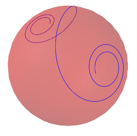
Refer to caption
Figure 1: Plot of the spherical clothoid for α=1\alpha=1 and s∈[−5,5]s\in[-5,5]

3.2 Derivation

We begin by investigating a loose end from the kinematic construction. The following system of equations describes the rolling without slipping and twisting of a unit sphere on a planar clothoid with scale factor α\alpha (see 3 in [15] and 29a in [16]) :

dd​s​(x~y~z~)=(00−sin⁡(α​s22)00cos⁡(α​s22)sin⁡(α​s22)−cos⁡(α​s22)0)​(x~y~z~)\frac{d}{ds}\begin{pmatrix}\tilde{x}\\ \tilde{y}\\ \tilde{z}\end{pmatrix}=\begin{pmatrix}0&0&-\sin\left(\frac{\alpha s^{2}}{2}\right)\\ 0&0&\cos\left(\frac{\alpha s^{2}}{2}\right)\\ \sin\left(\frac{\alpha s^{2}}{2}\right)&-\cos\left(\frac{\alpha s^{2}}{2}\right)&0\end{pmatrix}\begin{pmatrix}\tilde{x}\\ \tilde{y}\\ \tilde{z}\end{pmatrix} (9)

We introduce two new complex variables (see 10 in [15], 8 in [16]):

x~=a​b∗+b​a∗,y~=i⁡(a​b∗−b​a∗),z~=a​a∗−b​b∗.\tilde{x}=ab^{*}+ba^{*},\tilde{y}=\mathrm{i}\left(ab^{*}-ba^{*}\right),\tilde{z}=aa^{*}-bb^{*}. (10)

This tool was first presented by Feynman, Vernon and Hellwarth to geometrically represent the Schrödinger equation of a two-level quantum system [17]. aa and bb must satsfy the following system in order for x~\tilde{x},y~\tilde{y} and z~\tilde{z} to satisfy (9):

i​dd​s​(ab)=−12​(0e−iαs2/2ei​α​s2/20)​(ab)\mathrm{i}\frac{d}{ds}\begin{pmatrix}a\\ b\end{pmatrix}=-\frac{1}{2}\begin{pmatrix}0&e^{-\mathrm{i}\alpha s^{2}/2}\\ e^{\mathrm{i}\alpha s^{2}/2}&0\end{pmatrix}\begin{pmatrix}a\\ b\end{pmatrix} (11)

We are now left with a system that can be solved directly in a computer algebra system. Consult Appendix B for a solution using Mathematica. This system arises in the Landau-Zener problem (4, [18]). In fact, Zener first solved this system analytically using parabolic cylinder functions in this quantum physics context.
We then obtain the solution to Mehlum’s equation using (10) again and a rigid motion to satisfy the initial conditions.

3.3 Stereographic projection
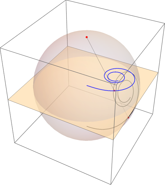
Refer to caption
Figure 2: Plot of the spherical clothoid and its stereographic projection for α=1\alpha=1 and s∈[0,5]s\in[0,5]

Stereographic projection is a mapping that projects the sphere onto the plane. Circles on the sphere are mapped to circles on the plane (as long as they do not pass through the point of projection) and loxodromes are mapped to logarithmic spirals. We shift the sphere to center it on the origin and consider the stereographic projection of our curve onto the complex plane:

ζ⁡(s)=X⁡(s)+i​Y​(s)=x⁡(s)+i​z​(s)1−(y⁡(s)−1)=s1​F1​(i8​α+12,32,i​α​s22)21​F1​(i8​α,12,i​α​s22)\begin{split}\zeta(s)&=X(s)+\mathrm{i}Y(s)\\ &=\frac{x(s)+\mathrm{i}z(s)}{1-(y(s)-1)}\\ &=\frac{s\,_{1}F_{1}\left(\frac{\mathrm{i}}{8\,\alpha}+\frac{1}{2},\frac{3}{2};\frac{\mathrm{i}\,\alpha s^{2}}{2}\right)}{2\,_{1}F_{1}\left(\frac{\mathrm{i}}{8\,\alpha},\frac{1}{2};\frac{\mathrm{i}\,\alpha s^{2}}{2}\right)}\end{split} (12)

We also have an alternative representation using a quotient of odd and even parabolic cylinder functions:

ζ⁡(s)=e−iπ/4y2(i4​α−12;ei​π/4αs)2​αy1​(i4​α−12,ei​π/4​α​s)\zeta(s)=\frac{e^{-\mathrm{i}\pi/4}\;y_{2}\left(\frac{\mathrm{i}}{4\alpha}-\frac{1}{2};e^{\mathrm{i}\pi/4}\sqrt{\alpha}s\right)}{2\sqrt{\alpha}\;\;\;\,y_{1}\left(\frac{\mathrm{i}}{4\alpha}-\frac{1}{2};e^{\mathrm{i}\pi/4}\sqrt{\alpha}s\right)} (13)

3.4 Humbert series corollaries

Let us revisit Mehlum and Wimp’s work on the spherical clothoid. We begin with Mehlum’s hypergeometric expression for yy restricted to the unit sphere (2.54 in [9]):

y⁡(s)=1−ϕ2​(i4​α,−i4​α,12,i​α​s22,−i​α​s22)y(s)=1-\phi_{2}\left(\frac{\mathrm{i}}{4\,\alpha},-\frac{\mathrm{i}}{4\,\alpha},\frac{1}{2};\frac{\mathrm{i}\,\alpha s^{2}}{2},-\frac{\mathrm{i}\,\alpha s^{2}}{2}\right) (14)

Combining this work with our new representation yields a novel reduction formula for a special form of ϕ2\phi_{2}:

ϕ2​(a,−a,12,x,−x)=21​F1​(a2,12,x)1​F1​(−a2,12,−x)−1\phi_{2}\left(a,-a,\frac{1}{2};x,-x\right)=2\,_{1}F_{1}\left(\frac{a}{2},\frac{1}{2};x\right)\,_{1}F_{1}\left(-\frac{a}{2},\frac{1}{2};-x\right)-1 (15)

We can use some suggestions in Mehlum’s work to obtain an expression for x+i​zx+\mathrm{i}z using ϕ1\phi_{1} special forms and less mysterious functions (see Appendix B for the derivation):

u=π​cos⁡(π​i4​α)​Γ​(−i4​α−12)i4​α​Γ​(−i8​α)2v=−π​cos⁡(π​i4​α)​Γ​(i4​α−12)2​Γ​(i8​α+12)2ϕ1=ϕ1​(i4​α+1,i4​α,i4​α+32,12,i​α​s22)ϕ1∗=ϕ1​(−i4​α+1,−i4​α,−i4​α+32,12,−i​α​s22)x⁡(s)+i​z​(s)=s⁡(u​e−i​α​s22​ϕ1+v​ei​α​s22​ϕ1∗)\begin{split}&u=\frac{\sqrt{\pi}\cos(\pi\frac{\mathrm{i}}{4\,\alpha})\Gamma\left(-\frac{\mathrm{i}}{4\,\alpha}-\frac{1}{2}\right)}{\frac{\mathrm{i}}{4\,\alpha}\Gamma\left(-\frac{\mathrm{i}}{8\,\alpha}\right)^{2}}\\ &v=-\frac{\sqrt{\pi}\cos(\pi\frac{\mathrm{i}}{4\,\alpha})\Gamma\left(\frac{\mathrm{i}}{4\,\alpha}-\frac{1}{2}\right)}{2\Gamma\left(\frac{\mathrm{i}}{8\,\alpha}+\frac{1}{2}\right)^{2}}\\ &\phi_{1}=\phi_{1}\left(\frac{\mathrm{i}}{4\,\alpha}+1,\frac{\mathrm{i}}{4\,\alpha},\frac{\mathrm{i}}{4\,\alpha}+\frac{3}{2};\frac{1}{2},\frac{\mathrm{i}\,\alpha s^{2}}{2}\right)\\ &\phi_{1}^{*}=\phi_{1}\left(-\frac{\mathrm{i}}{4\,\alpha}+1,-\frac{\mathrm{i}}{4\,\alpha},-\frac{\mathrm{i}}{4\,\alpha}+\frac{3}{2};\frac{1}{2},-\frac{\mathrm{i}\,\alpha s^{2}}{2}\right)\\ &x(s)+\mathrm{i}\,z(s)=s\left(u\,e^{-\frac{\mathrm{i}\,\alpha s^{2}}{2}}\phi_{1}+v\,e^{\frac{\mathrm{i}\,\alpha s^{2}}{2}}\phi_{1}^{*}\right)\end{split} (16)

Once again combining this with our new representation yields a new identity:

π​cos⁡(π​a)​Γ​(−a−12)a​Γ​(−a2)2​e−x​ϕ1​(a+1,a,a+32,12,x)−π​cos⁡(π​a)​Γ​(a−12)2​Γ​(a+12)2​ex​ϕ1​(−a+1,−a,−a+32,12,−x)=1F1(−a2,12;−x)1F1(a2+12,32;x)\begin{split}&\phantom{-}\frac{\sqrt{\pi}\cos(\pi a)\Gamma\left(-a-\frac{1}{2}\right)}{a\Gamma\left(-\frac{a}{2}\right)^{2}}e^{-x}\phi_{1}\left(a+1,a,a+\frac{3}{2};\frac{1}{2},x\right)\\ &-\frac{\sqrt{\pi}\cos(\pi a)\Gamma\left(a-\frac{1}{2}\right)}{2\Gamma\left(\frac{a+1}{2}\right)^{2}}e^{x}\phi_{1}\left(-a+1,-a,-a+\frac{3}{2};\frac{1}{2},-x\right)\\[8.5359pt] &\qquad\qquad\qquad=\,_{1}F_{1}\left(-\frac{a}{2},\frac{1}{2};-x\right)\,_{1}F_{1}\left(\frac{a}{2}+\frac{1}{2},\frac{3}{2};x\right)\end{split} (17)

It is interesting to note that these reductions demystify some quadratic relationships for special functions studied by Mehlum and Wimp (section 5 in [12]).

3.5 Generating function formulas related to the associated Meixner-Pollaczek polynomials

Mehlum found expressions for the parameter functions of the spherical clothoid involving associated Meixner-Pollaczek polynomials (2.38, 2.39 and 2.40 in [9]):

x⁡(s)=∑j=0∞Qj0​(14​α,π2,12)​(−α2)j​s2​j+1(1)jx(s)=\sum_{j=0}^{\infty}Q_{j}^{0}(\frac{1}{4\alpha};\frac{\pi}{2},\frac{1}{2})\frac{\left(\frac{-\alpha}{2}\right)^{j}s^{2j+1}}{(1)_{j}} (18)
y⁡(s)=12​∑j=0∞Qj0​(14​α,π2,1)​(−α2)j​s2​j+2(32)jy(s)=\frac{1}{2}\sum_{j=0}^{\infty}Q_{j}^{0}(\frac{1}{4\alpha};\frac{\pi}{2},1)\frac{\left(\frac{-\alpha}{2}\right)^{j}s^{2j+2}}{\left(\frac{3}{2}\right)_{j}} (19)
z⁡(s)=α6​∑j=0∞Qj0​(14​α,π2,32)​(−α2)j​s2​j+3(2)jz(s)=\frac{\alpha}{6}\sum_{j=0}^{\infty}Q_{j}^{0}(\frac{1}{4\alpha};\frac{\pi}{2},\frac{3}{2})\frac{\left(\frac{-\alpha}{2}\right)^{j}s^{2j+3}}{(2)_{j}} (20)

Generating functions related to this family of orthogonal polynomials arise in recent research [19, 20, 21]. Combining these expressions with our new parameter functions, we obtain the following generating function results:

∑j=0∞Qj0​(x,π2,12)​tjj!=12(1F1(−i​x2,12;it)1F1(i​x2+12,32;−it)+1F1(i​x2,12;−it)1F1(−i​x2+12,32;it))\begin{split}\sum_{j=0}^{\infty}Q_{j}^{0}(x;\frac{\pi}{2},\frac{1}{2})\frac{t^{j}}{j!}=&\frac{1}{2}\Bigg(\,_{1}F_{1}\left(-\frac{\mathrm{i}x}{2},\frac{1}{2};\mathrm{i}t\right)\,_{1}F_{1}\left(\frac{\mathrm{i}x}{2}+\frac{1}{2},\frac{3}{2};-\mathrm{i}t\right)\\ &+\,_{1}F_{1}\left(\frac{\mathrm{i}x}{2},\frac{1}{2};-\mathrm{i}t\right)\,_{1}F_{1}\left(-\frac{\mathrm{i}x}{2}+\frac{1}{2},\frac{3}{2};\mathrm{i}t\right)\Bigg)\end{split} (21)
∑j=0∞Qj0​(x,π2,1)​tj(32)j=F11​(i​x2,12,−i​t)1​F1​(−i​x2,12,i​t)−12​x​t\sum_{j=0}^{\infty}Q_{j}^{0}(x;\frac{\pi}{2},1)\frac{t^{j}}{\left(\frac{3}{2}\right)_{j}}=\frac{\,{}_{1}F_{1}\left(\frac{\mathrm{i}x}{2},\frac{1}{2};-\mathrm{i}t\right)\,_{1}F_{1}\left(-\frac{\mathrm{i}x}{2},\frac{1}{2};\mathrm{i}t\right)-1}{2xt} (22)
∑j=0∞Qj0​(x,π2,32)​tj(j+1)!=3​i2​t(1F1(−i​x2,12;it)1F1(i​x2+12,32;−it)−1F1(i​x2,12;−it)1F1(−i​x2+12,32;it))\begin{split}\sum_{j=0}^{\infty}Q_{j}^{0}(x;\frac{\pi}{2},\frac{3}{2})\frac{t^{j}}{(j+1)!}=&\frac{3\mathrm{i}}{2t}\Bigg(\,_{1}F_{1}\left(-\frac{\mathrm{i}x}{2},\frac{1}{2};\mathrm{i}t\right)\,_{1}F_{1}\left(\frac{\mathrm{i}x}{2}+\frac{1}{2},\frac{3}{2};-\mathrm{i}t\right)\\ &-\,_{1}F_{1}\left(\frac{\mathrm{i}x}{2},\frac{1}{2};-\mathrm{i}t\right)\,_{1}F_{1}\left(-\frac{\mathrm{i}x}{2}+\frac{1}{2},\frac{3}{2};\mathrm{i}t\right)\Bigg)\end{split} (23)

4 Conclusion

We have found simple expressions for the Cartesian coordinates of the spherical clothoid and its projection with some special function results as a bonus. It is remarkable that tools from quantum physics elucidate a classical problem. Suddenly this curve studied by Mehlum does not seem so exotic, heightening its potential in the world of computer aided geometric design. The computation of the special functions presented in this work presents an avenue for future research.

5 Acknowledgments

I would like to thank Dr. Zurab Silagadze for discussions that sparked the idea behind this hypergeometric reduction tied to the spherical clothoid. I am grateful to Dr. Khalid Ahbli, Dr. James Hateley, Max Kölbl and Dr. Robert Lewis for their attention and support during my research.

Appendix A ODE solution verification

In[1]:= x[s_]:=1/2 s Hypergeometric1F1[-(I/(8 α\alpha)),1/2,-((I α\alpha s^2)/2)] Hypergeometric1F1[1/2+I/(8 α\alpha),3/2,(I α\alpha s^2)/2]+1/2 s Hypergeometric1F1[I/(8 α\alpha),1/2,(I α\alpha s^2)/2] Hypergeometric1F1[1/2-I/(8 α\alpha),3/2,-((I α\alpha s^2)/2)]
In[2]:= y[s_]:=2-2 Hypergeometric1F1[-(I/(8 α\alpha)),1/2,-((I α\alpha s^2)/2)] Hypergeometric1F1[I/(8 α\alpha),1/2,(I α\alpha s^2)/2]
In[3]:= z[s_]:=1/(2 I) s Hypergeometric1F1[-(I/(8 α\alpha)),1/2,-((I α\alpha s^2)/2)] Hypergeometric1F1[1/2+I/(8 α\alpha),3/2,(I α\alpha s^2)/2]-1/(2 I) s Hypergeometric1F1[I/(8 α\alpha),1/2,(I α\alpha s^2)/2] Hypergeometric1F1[1/2-I/(8 α\alpha),3/2,-((I α\alpha s^2)/2)]
In[4]:= r[s_]:={x[s],y[s],z[s]}
In[5]:= r[0]
Out[5]= {0,0,0}
In[6]:= r’[0]
Out[6]= {1,0,0}
In[7]:= r”[0]
Out[7]= {0,1,0}
In[8]:= FullSimplify[r”’[0]]
Out[8]= {-1,0,α\alpha}
In[9]:= FullSimplify[r””[s]+(α\alpha^2 s^2 + 1) r”[s] + 3 α\alpha^2 s r’[s]]
Out[9]= {0,0,0}
Mathematica Session

Appendix B Complex differential equation system

Here we take an experimental approach and consider the following initial conditions: a⁡(0)=1,b⁡(0)=0a(0)=1,b(0)=0 (implying x~​(0)=0,y~​(0)=,z~​(0)=1\tilde{x}(0)=0,\tilde{y}(0)=,\tilde{z}(0)=1)

In[1]:=DSolve[{a’[s] == 1/2 I b[s] E^(1/2 (-I) α\alpha s^2), b’[s] == 1/2 I a[s] E^(1/2 I α\alpha s^2), a[0] == 1, b[0] == 0}, {a, b}, s]
Out[1]={{a -> Function[{s}, E^(-(1/2) I s^2 α\alpha) Hypergeometric1F1[-((-I - 4 α\alpha)/(8 α\alpha)), 1/2, 1/2 I s^2 α\alpha]], b -> Function[{s}, 1/2 s (I Hypergeometric1F1[1 - (-I - 4 α\alpha)/(8 α\alpha), 3/2, 1/2 I s^2 α\alpha] + 4 α\alpha Hypergeometric1F1[1 - (-I - 4 α\alpha)/(8 α\alpha), 3/2, 1/2 I s^2 α\alpha] - 4 α\alpha Hypergeometric1F1[-((-I - 4 α\alpha)/(8 α\alpha)) 1/2, 1/2 I s^2 α\alpha])]}}
In[2]:=FullSimplify[E^(-(1/2) I s^2 α\alpha) Hypergeometric1F1[-((-I - 4 α\alpha)/(8 α\alpha)), 1/2, 1/2 I s^2 α\alpha]]
Out[2]=Hypergeometric1F1[-(I/(8 α\alpha)), 1/2, -(1/2) I s^2 α\alpha]
In[3]:=FullSimplify[1/2 s (I Hypergeometric1F1[1 - (-I - 4 α\alpha)/(8 α\alpha), 3/2, 1/2 I s^2 α\alpha] + 4 α\alpha Hypergeometric1F1[1 - (-I - 4 α\alpha)/(8 α\alpha), 3/2, 1/2 I s^2 α\alpha] - 4 α\alpha Hypergeometric1F1[-((-I - 4 α\alpha)/(8 α\alpha)), 1/2, 1/2 I s^2 α\alpha])]
Out[3]= 1/2 I s Hypergeometric1F1[1/2 + I/(8 α\alpha), 3/2, 1/2 I s^2 α\alpha]
Mathematica Session

Appendix C Mehlum’s x+i​zx+\mathrm{i}\,z

Combining Mehlum’s expression for xx and zz (2.65 and 2.67 in [9]) and a Humbert series transform (2.61 and 2.62 in [9]), it is possible to obtain expressions of this form:

x⁡(s)+i​z​(s)=s⁡(u​e−i​α​s22​ϕ1+v​ei​α​s22​ϕ1∗)=s⁡(u​Ξ1+v​Ξ1∗)\begin{split}x(s)+\mathrm{i}\,z(s)&=s\left(u\,e^{-\frac{\mathrm{i}\,\alpha s^{2}}{2}}\phi_{1}+v\,e^{\frac{\mathrm{i}\,\alpha s^{2}}{2}}\phi_{1}^{*}\right)\\ &=s\left(u\,\Xi_{1}+v\,\Xi_{1}^{*}\right)\end{split} (24)

uu, vv do not depend on ss and these are the special forms of Ξ1\Xi_{1} we are playing with:

Ξ1=Ξ1​(i4​α,12,i4​α+1,i4​α+32,12,−i​α​s22)=∑m=0∞(12)m(i4​α+32)m​F12​(i4​α,i4​α+1,i4​α+32+m,12)​(−i​α​s22)mm!Ξ1∗=Ξ1​(−i4​α,12,−i4​α+1,−i4​α+32,12,i​α​s22)=∑m=0∞(12)m(−i4​α+32)m​F12​(−i4​α,−i4​α+1,−i4​α+32+m,12)​(i​α​s22)mm!\begin{split}\Xi_{1}&=\Xi_{1}\left(\frac{\mathrm{i}}{4\,\alpha},\frac{1}{2},\frac{\mathrm{i}}{4\,\alpha}+1,\frac{\mathrm{i}}{4\,\alpha}+\frac{3}{2};\frac{1}{2},-\frac{\mathrm{i}\,\alpha s^{2}}{2}\right)\\ &=\sum_{m=0}^{\infty}\frac{(\frac{1}{2})_{m}}{(\frac{\mathrm{i}}{4\,\alpha}+\frac{3}{2})_{m}}{}_{2}F_{1}(\frac{\mathrm{i}}{4\,\alpha},\frac{\mathrm{i}}{4\,\alpha}+1,\frac{\mathrm{i}}{4\,\alpha}+\frac{3}{2}+m;\frac{1}{2})\frac{(-\frac{\mathrm{i}\,\alpha s^{2}}{2})^{m}}{m!}\\ \Xi_{1}^{*}&=\Xi_{1}\left(-\frac{\mathrm{i}}{4\,\alpha},\frac{1}{2},-\frac{\mathrm{i}}{4\,\alpha}+1,-\frac{\mathrm{i}}{4\,\alpha}+\frac{3}{2};\frac{1}{2},\frac{\mathrm{i}\,\alpha s^{2}}{2}\right)\\ &=\sum_{m=0}^{\infty}\frac{(\frac{1}{2})_{m}}{(-\frac{\mathrm{i}}{4\,\alpha}+\frac{3}{2})_{m}}{}_{2}F_{1}(-\frac{\mathrm{i}}{4\,\alpha},-\frac{\mathrm{i}}{4\,\alpha}+1,-\frac{\mathrm{i}}{4\,\alpha}+\frac{3}{2}+m;\frac{1}{2})\frac{(\frac{\mathrm{i}\,\alpha s^{2}}{2})^{m}}{m!}\\ \end{split} (25)

Let’s examine the special forms of F12{}_{2}F_{1} that arise. We first recall some identities derived by Mitra (2.68 and 2.69 in [9]):

2F1(a,a+1,a+12;12)=πΓ(a+12)[1Γ​(a2+12)2+1Γ⁡(a2+1)​Γ​(a2)]_{2}F_{1}\left(a,a+1,a+\frac{1}{2};\frac{1}{2}\right)=\sqrt{\pi}\Gamma\left(a+\frac{1}{2}\right)\left[\frac{1}{\Gamma\left(\frac{a}{2}+\frac{1}{2}\right)^{2}}+\frac{1}{\Gamma\left(\frac{a}{2}+1\right)\Gamma\left(\frac{a}{2}\right)}\right] (26)
2F1(a,a+1,a+32;12)=2πΓ(a+32)[1Γ​(a2+12)2−1Γ⁡(a2+1)​Γ​(a2)]_{2}F_{1}\left(a,a+1,a+\frac{3}{2};\frac{1}{2}\right)=2\sqrt{\pi}\Gamma\left(a+\frac{3}{2}\right)\left[\frac{1}{\Gamma\left(\frac{a}{2}+\frac{1}{2}\right)^{2}}-\frac{1}{\Gamma\left(\frac{a}{2}+1\right)\Gamma\left(\frac{a}{2}\right)}\right] (27)

Using the contiguous relations of F12{}_{2}F_{1} we can deduce another relation:

2F1(a,a+1,a+52;12)=43πΓ(a+52)[1−4​aΓ​(a2+12)2+1+4​aΓ⁡(a2+1)​Γ​(a2)]_{2}F_{1}\left(a,a+1,a+\frac{5}{2};\frac{1}{2}\right)=\frac{4}{3}\sqrt{\pi}\Gamma\left(a+\frac{5}{2}\right)\left[\frac{1-4a}{\Gamma\left(\frac{a}{2}+\frac{1}{2}\right)^{2}}+\frac{1+4a}{\Gamma\left(\frac{a}{2}+1\right)\Gamma\left(\frac{a}{2}\right)}\right] (28)

Examining the first few terms in the Maclaurin series of s⁡(u​Ξ1+v​Ξ1∗)s\left(u\,\Xi_{1}+v\,\Xi_{1}^{*}\right) and our initial conditions, we can now find expressions for uu and vv explicitly in terms of the gamma function and more common functions. There are no terms with even powers of ss in our Maclaurin series and that satisfies the first and third initial conditions. We examine the second and fourth:

In[1]:= u=Sqrt[Pi]Cos[Pi I/(4 α\alpha)] Gamma[-I/(4 α\alpha)-1/2]/(I/(4 α\alpha)Gamma[-I/(8α\alpha)]^2)
In[2]:= v=-Sqrt[Pi]Cos[Pi I/(4 α\alpha)] Gamma[I/(4 α\alpha)-1/2]/(2Gamma[I/(8α\alpha)+1/2]^2)
In[3]:= b=2 Sqrt[Pi] Gamma[I/(4 α\alpha)+3/2](1/Gamma[I/(8α\alpha)+1/2]^2-1/(Gamma[I/(8α\alpha)+1]Gamma[I/(8α\alpha)]))
In[4]:= bstar=2 Sqrt[Pi] Gamma[-I/(4 α\alpha)+3/2](1/Gamma[-I/(8α\alpha)+1/2]^2-1/(Gamma[-I/(8α\alpha)+1]Gamma[-I/(8α\alpha)]))
In[5]:= FullSimplify[u b + v bstar]
Out[5]= 1
In[6]:= c=(1/2)/(I/(4 α\alpha)+3/2) 4/3 Sqrt[Pi] Gamma[I/(4 α\alpha)+5/2]((1-I/α\alpha)/Gamma[I/(8α\alpha)+1/2]^2+(1+I/α\alpha)/(Gamma[I/(8α\alpha)+1]Gamma[I/(8α\alpha)])) (-I α\alpha/2)
In[7]:= cstar=(1/2)/(-I/(4 α\alpha)+3/2) 4/3 Sqrt[Pi] Gamma[-I/(4 α\alpha)+5/2]((1+I/α\alpha)/Gamma[-I/(8α\alpha)+1/2]^2+(1-I/α\alpha)/(Gamma[-I/(8α\alpha)+1]Gamma[-I/(8α\alpha)])) (I α\alpha/2)
In[8]:= FullSimplify[Factorial[3](u c + v cstar)]
Out[8]= -1+I α\alpha
Mathematica Session

This shows us the unique values of uu and vv that satisfy our initial conditions.

References

  • [1] CF Gauss. Disquisitiones generales circa seriem infinitam… Commentationes societatis regiae scientiarum Gottingensis recentiores, 2:1–46, 1813.
  • [2] E.E. Kummer. De integralibus quibusdam definitis et seriebus infinitis. Journal für die reine und angewandte Mathematik, 1837(17):228–242, 1837.
  • [3] P. Humbert. Sur les fonctions hypercylindriques. C. R. Acad. Sci., Paris, 171:490–492, 1920.
  • [4] Bateman Manuscript Project, H. Bateman, A. Erdélyi, and United States. Office of Naval Research. Higher Transcendental Functions. Number vol. 1 in Bateman Manuscript Project California Institute of Technology. McGraw-Hill, 1953.
  • [5] Milton Abramowitz and Irene A. Stegun. Handbook of Mathematical Functions with Formulas, Graphs, and Mathematical Tables. Dover, New York, ninth dover printing, tenth gpo printing edition, 1964.
  • [6] Felix Pollaczek. Sur une famille de polynômes orthogonaux à quatre paramètres. C. R. Acad. Sci., Paris, 230:2254–2256, 1950.
  • [7] Min jie Luo and Ravinder Krishna Raina. Generating functions of pollaczek polynomials: a revisit. Integral Transforms and Special Functions, 30:893 – 919, 2019.
  • [8] Raphael Linus Levien. From Spiral to Spline: Optimal Techniques in Interactive Curve Design. PhD thesis, EECS Department, University of California, Berkeley, Dec 2009.
  • [9] Even Mehlum. Appell and the apple (nonlinear splines in space). In M. Dæhlen, T. Lyche, and L. L. Schumaker, editors, Mathematical Methods for Curves and Surfaces: Ulvik, Norway. Vanderbilt University Press, 1994.
  • [10] Josef Stoer. Curve fitting with clothoidal splines. J. Res. Nat. Bur. Standards, 87(4):317–346, 1982.
  • [11] Ian D. Coope. Curve interpolation with nonlinear spiral splines. IMA Journal of Numerical Analysis, 13(3):327–341, 1993.
  • [12] Even Mehlum and Jet Wimp. Spherical curves and quadratic relationships for special functions. The Journal of the Australian Mathematical Society. Series B. Applied Mathematics, 27(1):111–124, 1985.
  • [13] Erlend Grong Mauricio Godoy Molina. Geometric conditions for the existence of a rolling without twisting or slipping. Communications on Pure & Applied Analysis, 13(1):435–452, 2014.
  • [14] Ülo Lumiste. On submanifolds with parallel higher order fundamental form in euclidean spaces. In Dirk Ferus, Ulrich Pinkall, Udo Simon, and Berd Wegner, editors, Global Differential Geometry and Global Analysis, pages 126–137, Berlin, Heidelberg, 1991. Springer Berlin Heidelberg.
  • [15] Arkady Kholodenko and Zurab Silagadze. When physics helps mathematics: Calculation of the sophisticated multiple integral. Physics of Particles and Nuclei, 43, 01 2012.
  • [16] Alberto G. Rojo and Anthony M. Bloch. The rolling sphere, the quantum spin, and a simple view of the landau–zener problem. American Journal of Physics, 78(10):1014–1022, 2010.
  • [17] Richard P. Feynman, Frank L. Vernon, and Robert W. Hellwarth. Geometrical representation of the schrödinger equation for solving maser problems. Journal of Applied Physics, 28(1):49–52, 1957.
  • [18] Clarence Zener. Non-adiabatic crossing of energy levels. Proceedings of the Royal Society of London. Series A, Containing Papers of a Mathematical and Physical Character, 137(833):696–702, 1932.
  • [19] Min-Jie Luo, Ravinder Krishna Raina, and Shu-Han Zhao. Certain results on generating functions related to the associated meixner-pollaczek polynomials. Integral Transforms and Special Functions, 0(0):1–17, 2021.
  • [20] Khalid Ahbli and Zouhair Mouayn. A generating function and formulae defining the first-associated meixner-pollaczek polynomials. Integral Transforms and Special Functions, 29, 02 2018.
  • [21] Min-Jie Luo and Ravinder Krishna Raina. Generating functions of pollaczek polynomials: a revisit. Integral Transforms and Special Functions, 30(11):893–919, 2019.

E-mail address: alexandru.ionut172@gmail.com