Contrastive Learning of Sociopragmatic Meaning in Social Media
Abstract
Recent progress in representation and contrastive learning in NLP has not widely considered the class of sociopragmatic meaning (i.e., meaning in interaction within different language communities). To bridge this gap, we propose a novel framework for learning task-agnostic representations transferable to a wide range of sociopragmatic tasks (e.g., emotion, hate speech, humor, sarcasm). Our framework outperforms other contrastive learning frameworks for both in-domain and out-of-domain data, across both the general and few-shot settings. For example, compared to two popular pre-trained language models, our model obtains an improvement of average on datasets when fine-tuned on only training samples per dataset. We also show that our framework improves uniformity and preserves the semantic structure of representations. Our code is available at: https://github.com/UBC-NLP/infodcl
1 Introduction
Meaning emerging through human interaction such as on social media is deeply contextualized. It extends beyond referential meaning of utterances to involve both information about language users and their identity (the domain of sociolinguistics Tagliamonte 2015) and the communication goals of these users (the domain of pragmatics Thomas 2014). From a sociolinguistics perspective, a message can be expressed in various linguistic forms, depending on user background. For example, someone might say ‘let’s watch the soccer game’, but they can also call the game ‘football’. In real world, the game is the same thing. While the two expressions are different ways of saying the same thing Labov 1972, they do carry information about the user such as their region (i.e., where they could be coming from). From a pragmatics perspective, the meaning of an utterance depends on its interactive context. For example, while the utterance ‘it’s really hot here’ (said in a physical meeting) could be a polite way of asking someone to open the window, it could mean ‘it’s not a good idea for you to visit at this time’ (said in a phone conversation discussing travel plans). We refer to the meaning communicated through this type of socially embedded interaction as sociopragmatic meaning (SM).

While SM is an established concept in linguistics Leech 1983, NLP work still lags behind. This issue is starting to be acknowledged in the NLP community Nguyen et al. 2021, and there has been calls to include social aspects in representation learning of language Bisk et al. 2020. Arguably, pre-trained language models (PLMs) such as BERT Devlin et al. 2019 learn representations relevant to SM tasks. While this is true to some extent, PLMs are usually pre-trained on standard forms of language (e.g. BookCorpus) and hence miss (i) variation in language use among different language communities (social aspects of meaning) in (ii) interactive settings (pragmatic aspects). In spite of recent efforts to rectify some of these limitations by PLMs such as BERTweet on casual language Nguyen et al. 2020, it is not clear whether the masked language modeling (MLM) objective employed in PLMs is sufficient for capturing the rich representations needed for sociopragmatics.
Another common issue with PLMs is that their sequence-level embeddings suffer from the anisotropy problem Ethayarajh 2019; Li et al. 2020. That is, these representations tend to occupy a narrow cone on the multidimensional space. This makes it hard for effectively teasing apart sequences belonging to different classes without use of large amounts of labeled data. Work on contrastive learning (CL) has targeted this issue of anisotropy by attempting to bring semantic representations of instances of a given class (e.g., positive pairs of the same objects in images or same topics in text) closer and representations of negative class(es) instances farther away Liu et al. 2021a; Gao et al. 2021. A particularly effective type of CL is supervised CL Khosla et al. 2020; Khondaker et al. 2022, but it (i) requires labeled data (ii) for each downstream task. Again, acquiring labeled data is expensive and resulting models are task-specific (i.e., cannot be generalized to all SM tasks).
In this work, our goal is to learn effective task-agnostic representations for SM from social data without a need for labels. To achieve this goal, we introduce a novel framework situated in CL that we call InfoDCL. InfoDCL leverages sociopragmatic signals such as emojis or hashtags naturally occurring in social media, treating these as distant/surrogate labels.11 1 We use distant label and surrogate label interchangeably. Since surrogate labels are abundant (e.g., hashtags on images or videos), our framework can be extended beyond language. To illustrate the superiority of our proposed framework, we evaluate representations by our InfoDCL on SM datasets (such as emotion recognition Mohammad et al. 2018 and irony detection Ptácek et al. 2014) and compare against competitive baselines. Our proposed framework outperforms all baselines on (out of ) in-domain datasets and seven (out of eight) out-of-domain datasets (Sec. 4). Furthermore, our framework is strikingly successful in few-shot learning: it consistently outperforms baselines by a large margin for different sizes of training data (Sec. 4). Our framework is also language-independent, as demonstrated on several tasks from three languages other than English (Sec. E.3).
Our major contributions are as follows: (1) We introduce InfoDCL, a novel CL framework for learning sociopragmatics exploiting surrogate labels. To the best of our knowledge, this is the first work to utilize surrogate labels in language CL to improve PLMs. (2) We propose a new CL loss, Corpus-Aware Contrastive Loss (CCL), to preserve the semantic structure of representations exploiting corpus-level information (Sec. 3.3). (3) Our framework outperforms several competitive methods on a wide range of SM tasks (both in-domain and out-of-domain, across general and few-shot settings). (4) Our framework is language-independent, as demonstrated by its utility on various SM tasks in four languages. (5) We offer an extensive number of ablation studies that show the contribution of each component in our framework and qualitative analyses that demonstrate superiority of representation from our models (Sec. 5).
2 Related Work
Our work combines advances in representation learning and contrastive learning.
Representation Learning.
PLMs encode discrete language symbols into a continuous representation space that can capture the syntactic and the semantic information underlying the text. Since BERT is pre-trained on standard text that is not ideal for social media, Nguyen et al. 2020 propose BERTweet, a model pre-trained on tweets with MLM objective and without intentionally learning SM from social media data. Previous studies Felbo et al. 2017; Corazza et al. 2020 have also utilized distant supervision (e.g., use of emoji) to obtain better representations for a limited number of tasks. Our work differs in that we make use of distant supervision in the context of CL to acquire rich representations suited to the whole class of SM tasks. In addition, our methods excel not only in the full data setting but also for few-shot learning and diverse domains.
Contrastive Learning.
There has been a flurry of recent CL frameworks introducing self-supervised Liu et al. 2021a; Gao et al. 2021; Cao et al. 2022, semi-supervised Yu et al. 2021, weakly-supervised Zheng et al. 2021, and strongly supervised Gunel et al. 2021; Suresh and Ong 2021; Zhou et al. 2022 learning objectives.22 2 These frameworks differ across a number of dimensions that we summarize in Table 6 in Sec. A in Appendix. Although effective, existing supervised CL (SCL) frameworks Gunel et al. 2021; Suresh and Ong 2021; Pan et al. 2022 suffer from two major drawbacks. The first drawback is SCL’s dependence on task-specific labeled data (which is required to identify positive samples in a batch). Recently, Zheng et al. 2021 introduced a weakly-supervised CL (WCL) objective for computer vision, which generates a similarity-based 1-nearest neighbor graph in each batch and assigns weak labels for samples of the batch (thus clustering vertices in the graph). It is not clear, however, how much an WCL method with augmentations akin to language would fare for NLP. We propose a framework that does not require model-derived weak labels, which outperforms a clustering-based WCL approach. The second drawback with SCL is related to how negative samples are treated. Khosla et al. 2020; Gunel et al. 2021 treat all the negatives equally, which is sub-optimal since hard negatives should be more informative Robinson et al. 2021. Suresh and Ong 2021 attempt to rectify this by introducing a label-aware contrastive loss (LCL) where they feed the anchor sample to a task-specific model and assign higher weights to confusable negatives based on this model’s confidence on the class corresponding to the negative sample. LCL, however, is both narrow and costly. It is narrow since it exploits task-specific labels. We fix this by employing surrogate labels generalizable to all SM tasks. In addition, LCL is costly since it requires an auxiliary task-specific model to be trained with the main model. Again, we fix this issue by introducing a light LCL framework (LCL-LiT) where we use our main model, rather than an auxiliary model, to derive the weight vector from our main model through an additional loss (i.e., weighting is performed end-to-end in our main model). Also, LCL only considers instance-level information to capture relationships between individual sample and classes. In comparison, we introduce a novel corpus-aware contrastive loss (CCL) that overcomes this limitation (Sec. 3.3).
3 Proposed Framework
Our goal is to learn rich and diverse representations suited for a wide host of SM tasks. To this end, we introduce our novel InfoDCL framework. InfoDCL is a distantly supervised CL (DCL) framework that exploits distant/surrogate label (e.g., emoji) as a proxy for supervision and incorporates corpus-level information to capture inter-class relationships.
3.1 Contrastive Losses
CL aims to learn efficient representations by pulling samples from the same class together and pushing samples from other classes apart Hadsell et al. 2006. We formalize the framework now. Let denote the set of class labels. Let denote a randomly sampled batch of size , where and denote a sample and its label respectively. Many CL frameworks construct the similar (a.k.a., positive) sample () for an anchor sample () by applying a data augmentation technique () such as back-translation Fang and Xie 2020, token masking Liu et al. 2021a, and dropout masking Gao et al. 2021 on the anchor sample (). Let denote an augmented batch, where and = ().
Self-supervised Contrastive Loss.
We consider , where is the total number of training samples. Hence, the representation of the anchor sample is pulled closer to that of its augmented (positive) sample and pushed away from the representations of other (negative) samples in the batch. The semantic representation for each sample is computed by an encoder, , where . Chen et al. 2017 calculate the contrastive loss in a batch as follows:
| (1) |
where is the index of positive sample of ,33 3 If , , otherwise . is a scalar temperature parameter, and is the cosine similarity .
Supervised Contrastive Loss.
The CL loss in Eq. 1 is unable to handle the case of multiple samples belonging to the same class when utilizing a supervised dataset (). Positive samples in SCL Khosla et al. 2020 is a set composed of not only the augmented sample but also the samples belonging to the same class as . The positive samples of are denoted by , and is its cardinality. The SCL is formulated as:
| (2) |
In our novel framework, we make use of SCL but employ surrogate labels instead of gold labels to construct the positive set.
3.2 Label-Aware Contrastive Loss
Suresh and Ong 2021 extend the SCL to capture relations between negative samples. They hypothesize that not all negatives are equally difficult for an anchor and that the more confusable negatives should be emphasized in the loss. They propose LCL, which introduces a weight to indicate the confusability of class label w.r.t. anchor :
| (3) |
The weight vector comes from the class-specific probabilities (or confidence score) outputted by an auxiliary task-specific supervised model after consuming the anchor . LCL assumes that the highly confusable classes w.r.t anchor receive higher confidence scores, while the lesser confusable classes w.r.t anchor receive lower confidence scores. As stated earlier, limitations of LCL include (i) its dependence on gold annotations, (ii) its inability to generalize to all SM tasks due to its use of task-specific labels, and (iii) its ignoring of corpus-level and inter-class information. As explained in Sec. 2, we fix all these issues.
3.3 Corpus-Aware Contrastive Loss
In spite of the utility of existing CL methods for text representation, a uniformity-tolerance dilemma has been identified in vision representation model by Wang and Liu 2021: pursuing excessive uniformity makes a model intolerant to semantically similar samples, thereby breaking its underlying semantic structure (and thus causing harm to downstream performance).44
4
For details see Sec. G in Appendix. Our learning objective is to obtain representations suited to all SM tasks, thus we hypothesize that preserving the semantic relationships between surrogate labels during pre-training can benefit many of downstream SM tasks. Since we have a large number of fine-grained classes (i.e., surrogate labels), each class will not be equally distant from all other classes. For example, the class ‘
![[Uncaptioned image]](2203.07648v5/emojis/1f600.png) ’ shares similar semantics with the class ‘
’ shares similar semantics with the class ‘
![[Uncaptioned image]](2203.07648v5/emojis/1f606.png) ’, but is largely distant to the class ‘
’, but is largely distant to the class ‘
![[Uncaptioned image]](2203.07648v5/emojis/1f62d.png) ’. The texts with ‘
’ and ‘
’ belong to same class of ‘joy’ in downstream emotion detection task. We thus propose a new CL method that relies on distant supervision to learn general knowledge of all SM tasks and incorporates corpus-level information to capture inter-class relationships, while improving uniformity of PLM and preserving the underlying semantic structure. Concretely, our proposed corpus-aware contrastive loss (CCL) exploits a simple yet effective corpus-level measure based on pointwise mutual information (PMI) Bouma 2009 to extract relations between surrogate labels (e.g., emojis) from a large amount of unlabeled tweets.55
5
We experiment with a relatively sophisticated approach that learns class embeddings to capture the inter-class relations in Sec. 5, but find it to be sub-optimal. The PMI method is cheap to compute as it requires neither labeled data nor model training: PMI is based only on the co-occurrence of emoji pairs. We hypothesize that PMI scores of emoji pairs could provide globally useful semantic relations between emojis. Our CCL based on PMI
can be formulated as:
’. The texts with ‘
’ and ‘
’ belong to same class of ‘joy’ in downstream emotion detection task. We thus propose a new CL method that relies on distant supervision to learn general knowledge of all SM tasks and incorporates corpus-level information to capture inter-class relationships, while improving uniformity of PLM and preserving the underlying semantic structure. Concretely, our proposed corpus-aware contrastive loss (CCL) exploits a simple yet effective corpus-level measure based on pointwise mutual information (PMI) Bouma 2009 to extract relations between surrogate labels (e.g., emojis) from a large amount of unlabeled tweets.55
5
We experiment with a relatively sophisticated approach that learns class embeddings to capture the inter-class relations in Sec. 5, but find it to be sub-optimal. The PMI method is cheap to compute as it requires neither labeled data nor model training: PMI is based only on the co-occurrence of emoji pairs. We hypothesize that PMI scores of emoji pairs could provide globally useful semantic relations between emojis. Our CCL based on PMI
can be formulated as:
| (4) |
where the weight , and is normalized point-wise mutual information Bouma 2009 between and .66 6 Equation for NPMI is in Appendix B.1.
3.4 Overall Objective
To steer the encoder to learn representations that recognize corpus-level inter-class relations while distinguishing between classes, we combine our and .77 7 Note that operates over surrogate labels rather than task-specific downstream labels as in Suresh and Ong 2021, thereby allowing us to learn broad SM representations. The resulting loss, which we collectively refer to as distantly-supervised contrastive loss is given by:
| (5) |
where is a hyper-parameter that controls the relative importance of each of the contrastive losses. Our results show that a model trained with can achieve sizeable improvements over baselines (Table 1). For a more enhanced representation, our proposed framework also exploits a surrogate label prediction (SLP) objective where the encoder is jointly optimized for the emoji prediction task using cross entropy loss. Our employment of an SLP objective now allows us to weight the negatives in using classification probabilities from our main model rather than training an additional weighting model, another divergence from Suresh and Ong 2021. This new LCL framework is our LCL-LiT (for light LCL),88 8 The formula of LCL-LiT is the same as Eq. 3 (i.e., Loss of LCL). giving us a lighter DCL loss that we call DCL-LiT:
| (6) |
Our sharing strategy where a single model is trained end-to-end on an overall objective incorporating negative class weighting should also improve our model efficiency (e.g., training speed, energy efficiency). Our ablation study in Sec. 5 confirms that using the main model as the weighing network is effective for overall performance. To mitigate effect of any catastrophic forgetting of token-level knowledge, the proposed framework includes an MLM objective defined by .99 9 The Equations of and are listed in Appendix B.2 and B.3, respectively. The overall objective function of the proposed InfoDCL framework can be given by:
| (7) |
where and are the loss scaling factors. We also employ a mechanism for randomly re-pairing an anchor with a new positive sample at the beginning of each epoch. We describe this epoch-wise repairing in Appendix B.4.
| Task | RB | MLM | E-MLM | SLP | Mir-B | Sim-S | Sim-D | SCL | LCL | WCL | DCL | InfoD-R | BTw | InfoD-B | |
| CrisisOltea | 95.87 | 95.81 | 95.91 | 95.89 | 95.79 | 95.71 | 95.94 | 95.88 | 95.87 | 95.83 | 95.92 | 96.01 | 95.76 | 95.84 | |
| EmoMoham | 78.76 | 79.68 | 80.79 | 81.25 | 78.27 | 77.00 | 81.05 | 78.79 | 77.66 | 77.65 | 80.54 | 81.34 | 80.23 | 81.96 | |
| HateWas | 57.01 | 56.87 | 56.65 | 57.05 | 57.09 | 56.70 | 57.13 | 56.94 | 56.96 | 57.19 | 57.14 | 57.30 | 57.32 | 57.65 | |
| HateDav | 76.04 | 77.55 | 77.79 | 75.70 | 75.88 | 74.40 | 77.15 | 77.20 | 75.90 | 76.87 | 76.79 | 77.29 | 76.93 | 77.94 | |
| HateBas | 47.85 | 52.56 | 52.33 | 52.58 | 45.49 | 46.81 | 52.32 | 48.24 | 48.93 | 50.68 | 52.17 | 52.84 | 53.62 | 53.95 | |
| In-Domain | HumorMea | 93.28 | 93.62 | 93.73 | 93.31 | 93.37 | 91.55 | 93.42 | 92.82 | 93.00 | 92.45 | 94.13 | 93.75 | 94.43 | 94.04 |
| IronyHee-A | 72.87 | 74.15 | 75.94 | 76.89 | 70.62 | 66.40 | 75.36 | 73.58 | 73.86 | 71.24 | 77.15 | 76.31 | 77.03 | 78.72 | |
| IronyHee-B | 53.20 | 52.87 | 55.85 | 56.38 | 49.60 | 46.26 | 54.06 | 50.68 | 53.63 | 52.80 | 57.48 | 57.22 | 56.73 | 59.15 | |
| OffenseZamp | 79.93 | 80.75 | 80.72 | 80.07 | 78.79 | 77.28 | 80.80 | 79.96 | 80.75 | 79.48 | 79.94 | 81.21 | 79.35 | 79.83 | |
| SarcRiloff | 73.71 | 74.87 | 77.34 | 77.97 | 66.60 | 64.41 | 80.27 | 73.92 | 74.82 | 73.68 | 79.26 | 78.31 | 78.76 | 80.52 | |
| SarcPtacek | 95.99 | 95.87 | 96.02 | 95.89 | 95.62 | 95.27 | 96.07 | 95.89 | 95.62 | 95.72 | 96.13 | 96.10 | 96.40 | 96.67 | |
| SarcRajad | 85.21 | 86.19 | 86.38 | 86.89 | 84.31 | 84.06 | 87.20 | 85.18 | 84.74 | 85.89 | 87.45 | 87.00 | 87.13 | 87.20 | |
| SarcBam | 79.79 | 80.48 | 80.66 | 81.08 | 79.02 | 77.58 | 81.40 | 79.32 | 79.62 | 79.53 | 81.31 | 81.49 | 81.76 | 83.20 | |
| SentiRosen | 89.55 | 89.69 | 90.41 | 91.03 | 85.87 | 84.54 | 90.64 | 89.82 | 89.79 | 89.69 | 90.65 | 91.59 | 89.53 | 90.41 | |
| SentiThel | 71.41 | 71.31 | 71.50 | 71.79 | 71.23 | 70.11 | 71.68 | 70.57 | 70.10 | 71.30 | 71.73 | 71.87 | 71.64 | 71.98 | |
| StanceMoham | 69.44 | 69.47 | 70.50 | 69.54 | 66.23 | 64.96 | 70.48 | 69.14 | 69.55 | 70.33 | 69.74 | 71.13 | 68.33 | 68.22 | |
| Average | 76.24 | 76.98 | 77.66 | 77.71 | 74.61 | 73.32 | 77.81 | 76.12 | 76.30 | 76.27 | 77.97 | 78.17 | 77.81 | 78.58 | |
| EmotionWall | 66.51 | 66.02 | 67.89 | 67.28 | 62.33 | 59.59 | 67.68 | 66.56 | 67.55 | 63.99 | 68.36 | 68.41 | 64.48 | 65.61 | |
| Out-of-Domain | EmotionDem | 56.59 | 56.77 | 56.80 | 56.67 | 57.13 | 56.69 | 55.27 | 54.14 | 56.82 | 55.61 | 57.43 | 57.28 | 53.33 | 54.99 |
| SarcWalk | 67.50 | 66.16 | 67.42 | 68.78 | 63.95 | 59.39 | 65.04 | 66.98 | 66.93 | 65.46 | 67.39 | 68.45 | 67.27 | 67.30 | |
| SarcOra | 76.92 | 76.34 | 77.10 | 77.25 | 75.57 | 74.68 | 77.12 | 76.94 | 75.99 | 76.95 | 77.76 | 77.41 | 77.33 | 76.88 | |
| Senti-MR | 89.00 | 89.67 | 89.97 | 89.58 | 88.66 | 87.81 | 89.09 | 89.14 | 89.33 | 89.47 | 89.15 | 89.43 | 87.94 | 88.21 | |
| Senti-YT | 90.22 | 91.33 | 91.22 | 91.98 | 88.63 | 85.27 | 92.23 | 90.29 | 89.82 | 91.07 | 92.26 | 91.98 | 92.25 | 92.41 | |
| SST-5 | 54.96 | 55.83 | 56.15 | 55.94 | 54.18 | 52.84 | 55.09 | 55.33 | 54.28 | 55.30 | 56.00 | 56.37 | 55.74 | 55.93 | |
| SST-2 | 94.57 | 94.33 | 94.39 | 94.51 | 93.97 | 91.49 | 94.29 | 94.50 | 94.24 | 94.61 | 94.64 | 94.98 | 93.32 | 93.73 | |
| Average | 74.53 | 74.55 | 75.12 | 75.25 | 73.05 | 70.97 | 74.48 | 74.24 | 74.37 | 74.06 | 75.37 | 75.54 | 73.96 | 74.38 |
3.5 Data for Representation Learning
We exploit emojis as surrogate labels using an English language dataset with M tweets and a total of unique emojis (TweetEmoji-EN). In addition, we acquire representation learning data for (1) our experiments on three additional languages (i.e., Arabic, Italian, and Spanish) and to (2) investigate of the utility of hashtags as surrogate labels. More about how we develop TweetEmoji-EN and all our other representation learning data is in Appendix C.1.
3.6 Evaluation Data and Splits
In-Domain Data.
We collect English language Twitter datasets representing eight different SM tasks. These are (1) crisis awareness, (2) emotion recognition, (3) hateful and offensive language detection, (4) humor identification, (5) irony and sarcasm detection, (6) irony type identification, (7) sentiment analysis, and (8) stance detection. We also evaluate our framework on nine Twitter datasets, three from each of Arabic, Italian, and Spanish. More information about our English and multilingual datasets is in Appendix C.2.
Out-of-Domain Data.
We also identify eight datasets of SM involving emotion, sarcasm, and sentiment derived from outside the Twitter domain (e.g., data created by psychologists, debate fora, YouTube comments, movie reviews). We provide more information about these datasets in Appendix C.2.
Data Splits.
3.7 Implementation and Baselines
For experiments on English, we initialize our model with the pre-trained English RoBERTaBase.1010 10 For short, we refer to the official released English RoBERTaBase as RoBERTa in the rest of the paper. For multi-lingual experiments (reported in Appendix E.3), we use the pre-trained XLM-RoBERTaBase model Conneau et al. 2020 as our initial checkpoint. More details about these two models are in Appendix D.1. We tune hyper-parameters of our InfoDCL framework based on performance on development sets of downstream tasks, finding our model to be resilient to changes in these as detailed in Appendix D.3. To evaluate on downstream tasks, we fine-tune trained models on each task for five times with different random seeds and report the averaged model performance. Our main metric is macro-averaged score. To evaluate the overall ability of a model, we also report an aggregated metric that averages over the in-domain datasets, eight out-of-domain tasks, and the nine multi-lingual Twitter datasets, respectively.
NPMI Weighting Matrix.
We randomly sample M tweets from our original M Twitter dataset, each with at least two emojis. We extract all emojis in each tweet and count the frequencies of emojis as well as co-occurrences between emojis. To avoid noisy relatedness from low frequency pairs, we filter out emoji pairs whose co-occurrences are less than times. We employ Eq. 8 (Appendix B.1) to calculate NPMI for each emoji pair.
Baselines.
We compare our methods to baselines, as described in Appendix D.2.
4 Main Results
Table 1 shows our main results. We refer to our models trained with (Eq. 5) and (Eq. 7) in Table 1 as DCL and InfoDCL, respectively. We compare our models to baselines on the Twitter (in-domain) datasets and eight out-of-domain datasets.
In-Domain Results.
InfoDCL outperforms Baseline (1), i.e., fine-tuning original RoBERTa, on each of the in-domain datasets, with average improvement. InfoDCL also outperforms both the MLM and surrogate label prediction (SLP) methods with and average scores, respectively. Our proposed framework is thus able to learn more effective representations for SM. We observe that both Mirror-BERT and SimCSE-Self negatively impact downstream task performance, suggesting that while the excessive uniformity they result in is useful for semantic similarity tasks Gao et al. 2021; Liu et al. 2021a, it hurts downstream SM tasks.1111 11 The analyses in Sections 5 and E.6 illustrate this behavior. We observe that our proposed variant of SimCSE, SimCSE-Distant, achieves sizable improvements over both Mirror-BERT and SimCSE-Self ( and average , respectively). This further demonstrates effectiveness of our distantly supervised objectives. SimCSE-Distant, however, cannot surpass our proposed InfoDCL framework on average over all the tasks. We also note that InfoDCL outperforms SCL, LCL, and WCL with , , and average , respectively. Although our simplified model, i.e., DCL, underperforms InfoDCL with average , it outperforms all the baselines. Overall, our proposed models (DCL and InfoDCL) obtain best performance in out of tasks, and InfoDCL acquires the best average . We further investigate the relation between model performance and emoji presence, finding that our proposed approach not only improves tasks involving high amounts of emoji content (e.g., the test set of EmoMoham has tweets containing emojis) but also those without any emoji content (e.g., HateDav). 1212 12 Statistics of emoji presence of each downstream task is shown in Table 7 in Appendix. Compared to the original BERTweet, our InfoDCL-RoBERTa is still better ( higher ). This demonstrates not only effectiveness of our approach as compared to domain-specific models pre-trained simply with MLM, but also its data efficiency: BERTweet is pre-trained with more data (M tweets vs. only M for our model). Moreover, the BERTweet we continue training with our framework obtains an average improvement of (outperforms it on individual tasks). The results demonstrate that our framework can enhance the domain-specific PLM as well.
Out-of-Domain Results.
InfoDCL achieves an average improvement of ( = ) over the eight out-of-domain datasets compared to Baseline (1) as Table 1 shows. Our DCL and InfoDCL models also surpass all baselines on average, achieving highest on seven out of eight datasets. We notice the degradation of BERTweet when we evaluate on the out-of-domain data. Again, this shows generalizability of our proposed framework for leaning SM.
Significance Tests.
We conduct two types of significance test on our results, i.e., the classical paired student’s t-test Fisher 1936 and Almost Stochastic Order (ASO) Dror et al. 2019. The t-test shows that our InfoDCL-RoBERTa significantly () outperforms out of baselines (exceptions are SimCSE-Distant and BERTweet) on the average scores over in-domain datasets and baselines (exception is SLP) on the average scores over eight out-of-domain datasets. ASO concludes that InfoDCL-RoBERTa significantly () outperforms all baselines on both average scores of in-domain and out-of-domain datasets. InfoDCL-BERTweet also significantly ( by t-test, by ASO) outperforms BERTweet on the average scores. We report standard deviations of our results and significance tests in Appendix E.1.
Additional Results.
Comparisons to Individual SoTAs. We compare our models on each dataset to the task-specific SoTA model on that dataset, acquiring strong performance on the majority of these as we show in Table 12, Sec. E.2 in Appendix. Beyond English. We also demonstrate effectiveness and generalizability of our proposed framework on nine SM tasks in three additional languages in Sec. E.3. Beyond Emojis. To show the generalizability of our framework to surrogate labels other than emojis, we train DCL and InfoDCL with hashtags and observe comparable gains (Sec. E.4). Beyond Sociopragmatics. Although the main objective of our proposed framework is to improve model representation for SM, we also evaluate our models on two topic classification datasets and a sentence evaluation benchmark, SentEval Conneau and Kiela 2018. This allows us to show both strengths of our framework (i.e., improvements beyond SM) and its limitations (i.e., on textual semantic similarity). More about SentEval is in Appendix C.2, and results are in Sections E.5 and E.6.
Few-Shot Learning Results.
Since DCL and InfoDCL exploit an extensive set of cues, allowing them to capture a broad range of nuanced concepts of SM, we hypothesize they will be particularly effective in few-shot learning. We hence fine-tune our DCL, InfoDCL, strongest two baselines, and the original RoBERTa with varying amounts of downstream data.1313 13 Data splits for few-shot experiments are in Appendix C.2. As Table 2 shows, for in-domain tasks, with only and training samples per task, our InfoDCL-RoBERTa strikingly improves and points over the RoBERTa baseline, respectively. Similarly, InfoDCL-RoBERTa is and over RoBERTa with and training samples for out-of-domain tasks. These gains also persist when we compare our framework to all other strong baselines, including as we increase data sample size. Clearly, our proposed framework remarkably alleviates the challenge of labelled data scarcity even under severely few-shot settings.1414 14 We offer additional few-shot results in Appendix E.7.
| N | 20 | 100 | 500 | 1000 | |
| In-Domain | RoBERTa | 35.22 | 41.92 | 70.06 | 72.20 |
| BERTweet | 39.14 | 38.23 | 68.35 | 73.50 | |
| Ours (SimCSE-Distant) | 44.99 | 54.06 | 71.56 | 73.39 | |
| Ours (DCL) | 46.60 | 58.31 | 72.00 | 73.86 | |
| Ours (InfoDCL-RoBERTa) | 46.88 | 59.44 | 72.72 | 74.47 | |
| Ours (InfoDCL-BERTweet) | 45.29 | 52.64 | 71.31 | 74.03 | |
| Out-of-Domain | RoBERTa | 27.07 | 41.12 | 69.26 | 71.42 |
| BERTweet | 30.89 | 39.40 | 62.52 | 68.22 | |
| Ours (SimCSE-Distant) | 39.02 | 53.95 | 66.85 | 70.50 | |
| Ours (DCL) | 42.19 | 56.62 | 68.22 | 71.21 | |
| Ours (InfoDCL-RoBERTa) | 40.96 | 58.51 | 69.36 | 71.92 | |
| Ours (InfoDCL-BERTweet) | 38.72 | 48.87 | 65.64 | 69.25 |
5 Ablation Studies and Analyses
| Model | Avg | Diff |
| InfoDCL | 78.17 (0.19) | - |
| wo CCL | 77.75 (0.18) | -0.42 |
| wo LCL | 78.09 (0.28) | -0.08 |
| wo CCL & LCL | 77.98 (0.19) | -0.19 |
| wo SLP | 76.37 (0.35) | -0.80 |
| wo MLM | 77.12 (0.31) | -0.05 |
| wo SLP & MLM (Our DCL) | 77.97 (0.24) | -0.20 |
| wo EpW-RP | 78.00 (0.41) | -0.17 |
| w additional weighting model | 78.16 (0.21) | -0.02 |
| InfoDCL+Self-Aug | 77.79 (0.27) | -0.38 |
Ablation Studies. We investigate effectiveness of each of the ingredients in our proposed framework through ablation studies exploiting TweetEmoji-EN for pre-training. We evaluate on the in-domain SM datasets with the same hyper-parameters identified in Sec. D.3 and report results over five runs. As Table 3 shows, InfoDCL outperforms all other settings, demonstrating the utility of the various components in our model. Results show the SLP objective is the most important ingredient in InfoDCL (with a drop of average when removed). However, when we drop both SLP and MLM objectives, DCL (our second best proposed model) only loses as compared to InfoDCL. Results also show that our proposed CCL is more effective than LCL: CCL is second most important component and results in drop vs. only drop when ablating LCL. Interestingly, when we remove both CCL and LCL, the model is relatively less affected (i.e., drop) than when we remove CCL alone. We hypothesize this is the case since CCL and LCL are two somewhat opposing objectives: LCL tries to make individual samples distinguishable across confusable classes, while CCL tries to keep the semantic relations between confusable classes. Overall, our results show the utility of distantly supervised contrastive loss. Although distant labels are intrinsically noisy, our InfoDCL is able to mitigate this noise by using CCL and LCL losses. Our epoch-wise re-pairing (EpW-RP) strategy is also valuable, as removing it results in a drop of average . We believe EpW-RP helps regularize our model as we dynamically re-pair an anchor with a new positive pair for each training epoch. We also train an additional network to produce the weight vector, , in LCL loss as Suresh and Ong 2021 proposed instead of using our own main model to assign this weight vector end-to-end. We observe a slight drop of average with the additional model, showing the superiority of our end-to-end approach (which is less computational costly). We also adapt a simple self-augmentation method introduced by Liu et al. 2021a to our distant supervision setting: given an anchor , we acquire a positive set where is a sample with the same emoji as the anchor, is an augmented version (applying dropout and masking) of , and is an augmented version of . As Table 3 shows, InfoDCL+Self-Aug underperforms InfoDCL ( drop). We investigate further issues as to how to handle inter-class relations in our models and answer the following questions:
Should we cluster or push apart the large number of fine-grained (correlated) classes? In previous works, contrastive learning is used to push apart samples from different classes. Suresh and Ong 2021 propose the LCL to penalize samples that is more confusable. In this paper, we hypothesize that we should also incorporate inter-class relations into learning objectives (our CCL). Hence, we introduce the PMI score into SCL to scale down the loss of a pair belonging to semantically related classes (emojis) as defined in Section 3.3 (which should help cluster our fine-grained classes). Here, we investigate an alternative strategy where we explore using the PMI scores as weights to scale up the loss of a pair with related labels (which should keep the fine-grained emoji classes separate). Hence, we set where . We train RoBERTa on M random samples from the training set of TweetEmoji-EN with the overall loss function in Eq. 7, one time using this new weighting method and another time using the weighting method used in all our reported models so far: . Given these two ways to acquire in Eq. 4, we fine-tune the trained model on the Twitter tasks. Our results in Table 4 show the penalizing strategy to perform lower than our original clustering strategy reported in all experiments in this paper. We also present their performance on each dataset in Table 5.
| Method | Average | |
| PMI | 77.70 | |
| EC-Emb | 77.53 | |
| PMI | 77.39 | |
| EC-Emb | 77.36 |
| RB | |||||
| Method | PMI | CLS-emb | PMI | CLS-emb | |
| CrisisOltea | 95.93 | 95.93 | 95.88 | 95.95 | 95.87 |
| EmoMoham | 81.03 | 81.30 | 81.00 | 80.43 | 78.76 |
| HateWas | 57.26 | 57.16 | 57.35 | 57.26 | 57.01 |
| HateDav | 76.07 | 77.42 | 76.95 | 76.59 | 76.04 |
| HateBas | 51.86 | 50.47 | 52.04 | 51.68 | 47.85 |
| HumorMea | 93.77 | 93.66 | 93.65 | 93.53 | 93.28 |
| IronyHee-A | 75.39 | 73.95 | 74.09 | 74.32 | 72.87 |
| IronyHee-B | 57.02 | 55.50 | 56.99 | 55.10 | 53.20 |
| OffenseZamp | 80.29 | 80.89 | 81.08 | 80.81 | 79.93 |
| SarcRiloff | 76.73 | 75.90 | 72.45 | 74.64 | 73.71 |
| SarcPtacek | 96.01 | 95.98 | 95.99 | 95.73 | 95.99 |
| SarcRajad | 86.81 | 86.28 | 86.22 | 86.13 | 85.21 |
| SarcBam | 81.40 | 81.02 | 81.18 | 80.48 | 79.79 |
| SentiRosen | 91.30 | 91.64 | 91.45 | 91.95 | 89.55 |
| SentiThel | 71.72 | 71.71 | 72.02 | 71.65 | 71.44 |
| StanceMoham | 70.69 | 71.60 | 69.91 | 71.57 | 69.44 |
| Average | 77.70 | 77.53 | 77.39 | 77.36 | 76.24 |
Can we use the emoji class embedding (EC-Emb) for corpus-level weighting?
We experiment with using the embedding of the emoji class (EC-Emb) as an alternative weighting method in place of PMI. Namely, we train RoBERTa on SLP (using the training set of TweetEmoji-EN) for three epochs with a standard cross-entropy loss. We then extract weights of the last classification layer and use these weights as class embeddings, , where , is hidden dimension (i.e., ), and is the size of classes (i.e., ). The correlation of each pair of emojis is computed using cosine similarity, i.e., .1515
15
Self-similarity is set to . As Table 4 and 5 shows, using PMI scores performs slightly better than using class embeddings in both the clustering and penalizing strategies mentioned previously in the current section. For more intuition, we hand-pick three query emojis and manually compare the quality of similarity measures produced by both PMI and class embeddings for these. As Table 17 in Appendix shows, both PMI and EC-Emb are capable of capturing sensible correlations between emojis (although the embedding approach includes a few semantically distant emojis, such as the emoji ‘
’ being highly related to ‘
![[Uncaptioned image]](2203.07648v5/emojis/1f601.png) ’).
’).
Qualitative Analysis.
To further illustrate the effectiveness of the representation learned by InfoDCL, we compare a -SNE Van der Maaten and Hinton 2008 visualization of it to that of two strong baselines on two SM datasets.1616 16 Note that we use our model representations without downstream fine-tuning. Fig. 2 shows that our model has clearly learned to cluster the samples with similar semantics and separate semantically different clusters before fine-tuning on the gold downstream samples, for both in-domain and out-of-domain tasks. We provide more details about how we obtain the -SNE vitalization and provide another visualization study in Appendix F.2.


Uniformity-Tolerance Dilemma. Following Wang and Liu 2021, we investigate uniformity and tolerance of our models using Dev data of downstream tasks.1717 17 For details see Sec. G in Appendix. As Fig. 3 shows, unlike other models, our proposed DCL and InfoDCL models make a balance between uniformity and tolerance (which works best for SM).
6 Conclusion
We proposed InfoDCL, a novel framework for adapting PLMs to SM exploiting surrogate labels in contrastive learning. We demonstrated effectiveness of our framework on in-domain and eight out-of-domain datasets as well as nine non-English datasets. Our model outperforms strong baselines and exhibits strikingly powerful performance in few-shot learning.
7 Limitations
We identify the potential limitations of our work as follow: (1) Distant labels may not be available in every application domain (e.g., patient notes in clinical application), although domain adaptation can be applied in these scenarios. We also believe that distantly supervised contrastive learning can be exploited in tasks involving image and video where surrogate labels are abundant. (2) We also acknowledge that the offline NPMI matrix of our proposed CCL method depends on a dataset (distantly) labeled with multiple classes in each sample. To alleviate this limitation, we explore an alternative method that uses learned class embeddings to calculate the inter-class relations in Section 5. This weighting approach achieves sizable improvement over RoBERTa on in-domain datasets, though it underperforms our NPMI-based approach. (3) Our framework does not always work on tasks outside SM. For example, our model underperforms self-supervised CL models, i.e., SimCSE-Self and Mirror-BERT, on semantic textual similarity task in Appendix E.6. As we showed, however, our framework exhibits promising performance on some other tasks. For example, our hashtag-based model acquires best performance on the topic classification task, as shown in Appendix E.5.
Ethical Considerations
All our evaluation datasets are collected from publicly available sources. Following privacy protection policy, all the data we used for model pre-training and fine-tuning are anonymized. Some annotations in the downstream data (e.g., for hate speech tasks) can carry annotator bias. We will accompany our data and model release with model cards. We will also provide more detailed ethical considerations on a dedicated GitHub repository. All our models will be distributed for research with a clear purpose justification.
Acknowledgements
We gratefully acknowledge support from the Natural Sciences and Engineering Research Council of Canada (NSERC; RGPIN-2018-04267), the Social Sciences and Humanities Research Council of Canada (SSHRC; 435-2018-0576; 895-2020-1004; 895-2021-1008), Canadian Foundation for Innovation (CFI; 37771), Digital Research Alliance of Canada (the Alliance),1818 18 https://www.computecanada.ca and UBC ARC-Sockeye.1919 19 https://arc.ubc.ca/ubc-arc-sockeye Any opinions, conclusions or recommendations expressed in this material are those of the author(s) and do not necessarily reflect the views of NSERC, SSHRC, CFI, the Alliance, or UBC ARC-Sockeye.
References
- Abdul-Mageed et al. (2020) Muhammad Abdul-Mageed, Chiyu Zhang, Azadeh Hashemi, and El Moatez Billah Nagoudi. 2020. AraNet: A deep learning toolkit for Arabic social media. In Proceedings of the 4th Workshop on Open-Source Arabic Corpora and Processing Tools, with a Shared Task on Offensive Language Detection, pages 16–23, Marseille, France. European Language Resource Association.
- Agirre et al. (2015) Eneko Agirre, Carmen Banea, Claire Cardie, Daniel M. Cer, Mona T. Diab, Aitor Gonzalez-Agirre, Weiwei Guo, Iñigo Lopez-Gazpio, Montse Maritxalar, Rada Mihalcea, German Rigau, Larraitz Uria, and Janyce Wiebe. 2015. Semeval-2015 task 2: Semantic textual similarity, english, spanish and pilot on interpretability. In Proceedings of the 9th International Workshop on Semantic Evaluation, SemEval@NAACL-HLT 2015, Denver, Colorado, USA, June 4-5, 2015, pages 252–263. The Association for Computer Linguistics.
- Agirre et al. (2014) Eneko Agirre, Carmen Banea, Claire Cardie, Daniel M. Cer, Mona T. Diab, Aitor Gonzalez-Agirre, Weiwei Guo, Rada Mihalcea, German Rigau, and Janyce Wiebe. 2014. Semeval-2014 task 10: Multilingual semantic textual similarity. In Proceedings of the 8th International Workshop on Semantic Evaluation, SemEval@COLING 2014, Dublin, Ireland, August 23-24, 2014, pages 81–91. The Association for Computer Linguistics.
- Agirre et al. (2012) Eneko Agirre, Daniel M. Cer, Mona T. Diab, and Aitor Gonzalez-Agirre. 2012. Semeval-2012 task 6: A pilot on semantic textual similarity. In Proceedings of the 6th International Workshop on Semantic Evaluation, SemEval@NAACL-HLT 2012, Montréal, Canada, June 7-8, 2012, pages 385–393. The Association for Computer Linguistics.
- Agirre et al. (2013) Eneko Agirre, Daniel M. Cer, Mona T. Diab, Aitor Gonzalez-Agirre, and Weiwei Guo. 2013. *sem 2013 shared task: Semantic textual similarity. In Proceedings of the Second Joint Conference on Lexical and Computational Semantics, *SEM 2013, June 13-14, 2013, Atlanta, Georgia, USA, pages 32–43. Association for Computational Linguistics.
- Agirre et al. (2016) Eneko Agirre, Aitor Gonzalez-Agirre, Iñigo Lopez-Gazpio, Montse Maritxalar, German Rigau, and Larraitz Uria. 2016. Semeval-2016 task 2: Interpretable semantic textual similarity. In Proceedings of the 10th International Workshop on Semantic Evaluation, SemEval@NAACL-HLT 2016, San Diego, CA, USA, June 16-17, 2016, pages 512–524. The Association for Computer Linguistics.
- Bamman and Smith (2015) David Bamman and Noah A. Smith. 2015. Contextualized sarcasm detection on twitter. In Proceedings of the Ninth International Conference on Web and Social Media, ICWSM 2015, University of Oxford, Oxford, UK, May 26-29, 2015, pages 574–577. AAAI Press.
- Barbieri et al. (2020) Francesco Barbieri, José Camacho-Collados, Luis Espinosa Anke, and Leonardo Neves. 2020. TweetEval: Unified benchmark and comparative evaluation for tweet classification. In Findings of the Association for Computational Linguistics: EMNLP 2020, Online Event, 16-20 November 2020, volume EMNLP 2020 of Findings of ACL, pages 1644–1650. Association for Computational Linguistics.
- Barbieri et al. (2018) Francesco Barbieri, José Camacho-Collados, Francesco Ronzano, Luis Espinosa Anke, Miguel Ballesteros, Valerio Basile, Viviana Patti, and Horacio Saggion. 2018. Semeval 2018 task 2: Multilingual emoji prediction. In Proceedings of The 12th International Workshop on Semantic Evaluation, SemEval@NAACL-HLT 2018, New Orleans, Louisiana, USA, June 5-6, 2018, pages 24–33. Association for Computational Linguistics.
- Basile et al. (2019) Valerio Basile, Cristina Bosco, Elisabetta Fersini, Debora Nozza, Viviana Patti, Francisco Manuel Rangel Pardo, Paolo Rosso, and Manuela Sanguinetti. 2019. SemEval-2019 task 5: Multilingual detection of hate speech against immigrants and women in Twitter. In Proceedings of the 13th International Workshop on Semantic Evaluation, SemEval@NAACL-HLT 2019, Minneapolis, MN, USA, June 6-7, 2019, pages 54–63. Association for Computational Linguistics.
- Bianchi et al. (2021) Federico Bianchi, Debora Nozza, and Dirk Hovy. 2021. FEEL-IT: emotion and sentiment classification for the italian language. In Proceedings of the Eleventh Workshop on Computational Approaches to Subjectivity, Sentiment and Social Media Analysis, WASSA@EACL 2021, Online, April 19, 2021, pages 76–83. Association for Computational Linguistics.
- Bisk et al. (2020) Yonatan Bisk, Ari Holtzman, Jesse Thomason, Jacob Andreas, Yoshua Bengio, Joyce Chai, Mirella Lapata, Angeliki Lazaridou, Jonathan May, Aleksandr Nisnevich, Nicolas Pinto, and Joseph Turian. 2020. Experience grounds language. In Proceedings of the 2020 Conference on Empirical Methods in Natural Language Processing (EMNLP), pages 8718–8735, Online. Association for Computational Linguistics.
- Bosco et al. (2018) Cristina Bosco, Felice Dell’Orletta, Fabio Poletto, Manuela Sanguinetti, and Maurizio Tesconi. 2018. Overview of the EVALITA 2018 hate speech detection task. In Proceedings of the Sixth Evaluation Campaign of Natural Language Processing and Speech Tools for Italian. Final Workshop (EVALITA 2018) co-located with the Fifth Italian Conference on Computational Linguistics (CLiC-it 2018), Turin, Italy, December 12-13, 2018, volume 2263 of CEUR Workshop Proceedings. CEUR-WS.org.
- Bouma (2009) Gerlof Bouma. 2009. Normalized (pointwise) mutual information in collocation extraction. Proceedings of GSCL, 30:31–40.
- Cao et al. (2022) Rui Cao, Yihao Wang, Yuxin Liang, Ling Gao, Jie Zheng, Jie Ren, and Zheng Wang. 2022. Exploring the impact of negative samples of contrastive learning: A case study of sentence embedding. In Findings of the Association for Computational Linguistics: ACL 2022, pages 3138–3152. Association for Computational Linguistics.
- Cer et al. (2017) Daniel Cer, Mona Diab, Eneko Agirre, Iñigo Lopez-Gazpio, and Lucia Specia. 2017. SemEval-2017 task 1: Semantic textual similarity multilingual and crosslingual focused evaluation. In Proceedings of the 11th International Workshop on Semantic Evaluation (SemEval-2017), pages 1–14, Vancouver, Canada. Association for Computational Linguistics.
- Chen et al. (2017) Ting Chen, Yizhou Sun, Yue Shi, and Liangjie Hong. 2017. On sampling strategies for neural network-based collaborative filtering. In Proceedings of the 23rd ACM SIGKDD International Conference on Knowledge Discovery and Data Mining, Halifax, NS, Canada, August 13 - 17, 2017, pages 767–776. ACM.
- Cignarella et al. (2018) Alessandra Teresa Cignarella, Simona Frenda, Valerio Basile, Cristina Bosco, Viviana Patti, and Paolo Rosso. 2018. Overview of the EVALITA 2018 task on irony detection in italian tweets (ironita). In Proceedings of the Sixth Evaluation Campaign of Natural Language Processing and Speech Tools for Italian. Final Workshop (EVALITA 2018) co-located with the Fifth Italian Conference on Computational Linguistics (CLiC-it 2018), Turin, Italy, December 12-13, 2018, volume 2263 of CEUR Workshop Proceedings. CEUR-WS.org.
- Conneau et al. (2020) Alexis Conneau, Kartikay Khandelwal, Naman Goyal, Vishrav Chaudhary, Guillaume Wenzek, Francisco Guzmán, Edouard Grave, Myle Ott, Luke Zettlemoyer, and Veselin Stoyanov. 2020. Unsupervised cross-lingual representation learning at scale. In Proceedings of the 58th Annual Meeting of the Association for Computational Linguistics, ACL 2020, Online, July 5-10, 2020, pages 8440–8451. Association for Computational Linguistics.
- Conneau and Kiela (2018) Alexis Conneau and Douwe Kiela. 2018. Senteval: An evaluation toolkit for universal sentence representations. In Proceedings of the Eleventh International Conference on Language Resources and Evaluation, LREC 2018, Miyazaki, Japan, May 7-12, 2018. European Language Resources Association (ELRA).
- Corazza et al. (2020) Michele Corazza, Stefano Menini, Elena Cabrio, Sara Tonelli, and Serena Villata. 2020. Hybrid emoji-based masked language models for zero-shot abusive language detection. In Findings of the Association for Computational Linguistics: EMNLP 2020, Online Event, 16-20 November 2020, volume EMNLP 2020 of Findings of ACL, pages 943–949. Association for Computational Linguistics.
- Corso et al. (2005) Gianna M. Del Corso, Antonio Gulli, and Francesco Romani. 2005. Ranking a stream of news. In Proceedings of the 14th international conference on World Wide Web, WWW 2005, Chiba, Japan, May 10-14, 2005, pages 97–106. ACM.
- Daouadi et al. (2021) Kheir Eddine Daouadi, Rim Zghal Rebaï, and Ikram Amous. 2021. Optimizing semantic deep forest for tweet topic classification. Inf. Syst., 101:101801.
- Davidson et al. (2017) Thomas Davidson, Dana Warmsley, Michael W. Macy, and Ingmar Weber. 2017. Automated hate speech detection and the problem of offensive language. In Proceedings of the Eleventh International Conference on Web and Social Media, ICWSM 2017, Montréal, Québec, Canada, May 15-18, 2017, pages 512–515. AAAI Press.
- Demszky et al. (2020) Dorottya Demszky, Dana Movshovitz-Attias, Jeongwoo Ko, Alan S. Cowen, Gaurav Nemade, and Sujith Ravi. 2020. Goemotions: A dataset of fine-grained emotions. In Proceedings of the 58th Annual Meeting of the Association for Computational Linguistics, ACL 2020, Online, July 5-10, 2020, pages 4040–4054. Association for Computational Linguistics.
- Devlin et al. (2019) Jacob Devlin, Ming-Wei Chang, Kenton Lee, and Kristina Toutanova. 2019. BERT: pre-training of deep bidirectional transformers for language understanding. In Proceedings of the 2019 Conference of the North American Chapter of the Association for Computational Linguistics: Human Language Technologies, NAACL-HLT 2019, Minneapolis, MN, USA, June 2-7, 2019, Volume 1 (Long and Short Papers), pages 4171–4186. Association for Computational Linguistics.
- Dolan and Brockett (2005) William B. Dolan and Chris Brockett. 2005. Automatically constructing a corpus of sentential paraphrases. In Proceedings of the Third International Workshop on Paraphrasing, IWP@IJCNLP 2005, Jeju Island, Korea, October 2005, 2005. Asian Federation of Natural Language Processing.
- Dror et al. (2019) Rotem Dror, Segev Shlomov, and Roi Reichart. 2019. Deep dominance - how to properly compare deep neural models. In Proceedings of the 57th Annual Meeting of the Association for Computational Linguistics, pages 2773–2785, Florence, Italy. Association for Computational Linguistics.
- Ethayarajh (2019) Kawin Ethayarajh. 2019. How contextual are contextualized word representations? Comparing the geometry of BERT, ELMo, and GPT-2 embeddings. In Proceedings of the 2019 Conference on Empirical Methods in Natural Language Processing and the 9th International Joint Conference on Natural Language Processing (EMNLP-IJCNLP), pages 55–65, Hong Kong, China. Association for Computational Linguistics.
- Fang and Xie (2020) Hongchao Fang and Pengtao Xie. 2020. CERT: contrastive self-supervised learning for language understanding. CoRR, abs/2005.12766.
- Felbo et al. (2017) Bjarke Felbo, Alan Mislove, Anders Søgaard, Iyad Rahwan, and Sune Lehmann. 2017. Using millions of emoji occurrences to learn any-domain representations for detecting sentiment, emotion and sarcasm. In Proceedings of the 2017 Conference on Empirical Methods in Natural Language Processing, EMNLP 2017, Copenhagen, Denmark, September 9-11, 2017, pages 1615–1625. Association for Computational Linguistics.
- Fisher (1936) Ronald Aylmer Fisher. 1936. Design of experiments. British Medical Journal, 1(3923):554.
- Gao et al. (2021) Tianyu Gao, Xingcheng Yao, and Danqi Chen. 2021. Simcse: Simple contrastive learning of sentence embeddings. In Proceedings of the 2021 Conference on Empirical Methods in Natural Language Processing, EMNLP 2021, Virtual Event / Punta Cana, Dominican Republic, 7-11 November, 2021, pages 6894–6910. Association for Computational Linguistics.
- Ghanem et al. (2019) Bilal Ghanem, Jihen Karoui, Farah Benamara, Véronique Moriceau, and Paolo Rosso. 2019. IDAT at FIRE2019: overview of the track on irony detection in arabic tweets. In FIRE ’19: Forum for Information Retrieval Evaluation, Kolkata, India, December, 2019, pages 10–13. ACM.
- Giorgi et al. (2021) John M. Giorgi, Osvald Nitski, Bo Wang, and Gary D. Bader. 2021. Declutr: Deep contrastive learning for unsupervised textual representations. In Proceedings of the 59th Annual Meeting of the Association for Computational Linguistics and the 11th International Joint Conference on Natural Language Processing, ACL/IJCNLP 2021, (Volume 1: Long Papers), Virtual Event, August 1-6, 2021, pages 879–895. Association for Computational Linguistics.
- Gunel et al. (2021) Beliz Gunel, Jingfei Du, Alexis Conneau, and Veselin Stoyanov. 2021. Supervised contrastive learning for pre-trained language model fine-tuning. In 9th International Conference on Learning Representations, ICLR 2021, Virtual Event, Austria, May 3-7, 2021. OpenReview.net.
- Hadsell et al. (2006) Raia Hadsell, Sumit Chopra, and Yann LeCun. 2006. Dimensionality reduction by learning an invariant mapping. In 2006 IEEE Computer Society Conference on Computer Vision and Pattern Recognition (CVPR 2006), 17-22 June 2006, New York, NY, USA, pages 1735–1742. IEEE Computer Society.
- Hee et al. (2018) Cynthia Van Hee, Els Lefever, and Véronique Hoste. 2018. Semeval-2018 task 3: Irony detection in english tweets. In Proceedings of The 12th International Workshop on Semantic Evaluation, SemEval@NAACL-HLT 2018, New Orleans, Louisiana, USA, June 5-6, 2018, pages 39–50. Association for Computational Linguistics.
- Hu and Liu (2004) Minqing Hu and Bing Liu. 2004. Mining and summarizing customer reviews. In Proceedings of the Tenth ACM SIGKDD International Conference on Knowledge Discovery and Data Mining, Seattle, Washington, USA, August 22-25, 2004, pages 168–177. ACM.
- Ke et al. (2020) Pei Ke, Haozhe Ji, Siyang Liu, Xiaoyan Zhu, and Minlie Huang. 2020. SentiLARE: Sentiment-aware language representation learning with linguistic knowledge. In Proceedings of the 2020 Conference on Empirical Methods in Natural Language Processing, EMNLP 2020, Online, November 16-20, 2020, pages 6975–6988. Association for Computational Linguistics.
- Khondaker et al. (2022) Md Tawkat Islam Khondaker, El Moatez Billah Nagoudi, AbdelRahim Elmadany, Muhammad Abdul-Mageed, and Laks Lakshmanan, V.S. 2022. A benchmark study of contrastive learning for Arabic social meaning. In Proceedings of the The Seventh Arabic Natural Language Processing Workshop (WANLP), pages 63–75, Abu Dhabi, United Arab Emirates (Hybrid). Association for Computational Linguistics.
- Khosla et al. (2020) Prannay Khosla, Piotr Teterwak, Chen Wang, Aaron Sarna, Yonglong Tian, Phillip Isola, Aaron Maschinot, Ce Liu, and Dilip Krishnan. 2020. Supervised contrastive learning. In Advances in Neural Information Processing Systems 33: Annual Conference on Neural Information Processing Systems 2020, NeurIPS 2020, December 6-12, 2020, virtual.
- Labov (1972) William Labov. 1972. Sociolinguistic patterns. 4. University of Pennsylvania press.
- Leech (1983) Geoffrey N Leech. 1983. Principles of pragmatics. London: Longman.
- Li et al. (2020) Bohan Li, Hao Zhou, Junxian He, Mingxuan Wang, Yiming Yang, and Lei Li. 2020. On the sentence embeddings from pre-trained language models. In Proceedings of the 2020 Conference on Empirical Methods in Natural Language Processing (EMNLP), pages 9119–9130, Online. Association for Computational Linguistics.
- Liu et al. (2021a) Fangyu Liu, Ivan Vulic, Anna Korhonen, and Nigel Collier. 2021a. Fast, effective, and self-supervised: Transforming masked language models into universal lexical and sentence encoders. In Proceedings of the 2021 Conference on Empirical Methods in Natural Language Processing, EMNLP 2021, Virtual Event / Punta Cana, Dominican Republic, 7-11 November, 2021, pages 1442–1459. Association for Computational Linguistics.
- Liu et al. (2021b) Junhua Liu, Trisha Singhal, Luciënne T. M. Blessing, Kristin L. Wood, and Kwan Hui Lim. 2021b. CrisisBERT: A robust transformer for crisis classification and contextual crisis embedding. In HT ’21: 32nd ACM Conference on Hypertext and Social Media, Virtual Event, Ireland, 30 August 2021 - 2 September 2021, pages 133–141. ACM.
- Liu et al. (2019) Yinhan Liu, Myle Ott, Naman Goyal, Jingfei Du, Mandar Joshi, Danqi Chen, Omer Levy, Mike Lewis, Luke Zettlemoyer, and Veselin Stoyanov. 2019. RoBERTa: A robustly optimized BERT pretraining approach. CoRR, abs/1907.11692.
- Marelli et al. (2014) Marco Marelli, Stefano Menini, Marco Baroni, Luisa Bentivogli, Raffaella Bernardi, and Roberto Zamparelli. 2014. A SICK cure for the evaluation of compositional distributional semantic models. In Proceedings of the Ninth International Conference on Language Resources and Evaluation, LREC 2014, Reykjavik, Iceland, May 26-31, 2014, pages 216–223. European Language Resources Association (ELRA).
- Meaney et al. (2021) J. A. Meaney, Steven R. Wilson, Luis Chiruzzo, Adam Lopez, and Walid Magdy. 2021. Semeval 2021 task 7: Hahackathon, detecting and rating humor and offense. In Proceedings of the 15th International Workshop on Semantic Evaluation, SemEval@ACL/IJCNLP 2021, Virtual Event / Bangkok, Thailand, August 5-6, 2021, pages 105–119. Association for Computational Linguistics.
- Meng et al. (2021) Yu Meng, Chenyan Xiong, Payal Bajaj, saurabh tiwary, Paul Bennett, Jiawei Han, and XIA SONG. 2021. Coco-lm: Correcting and contrasting text sequences for language model pretraining. In Advances in Neural Information Processing Systems, volume 34, pages 23102–23114. Curran Associates, Inc.
- Miller (1995) George A. Miller. 1995. Wordnet: A lexical database for english. Commun. ACM, 38(11):39–41.
- Mohammad et al. (2018) Saif Mohammad, Felipe Bravo-Marquez, Mohammad Salameh, and Svetlana Kiritchenko. 2018. Semeval-2018 task 1: Affect in tweets. In Proceedings of The 12th International Workshop on Semantic Evaluation, SemEval@NAACL-HLT 2018, New Orleans, Louisiana, USA, June 5-6, 2018, pages 1–17. Association for Computational Linguistics.
- Mohammad et al. (2016) Saif Mohammad, Svetlana Kiritchenko, Parinaz Sobhani, Xiao-Dan Zhu, and Colin Cherry. 2016. Semeval-2016 task 6: Detecting stance in tweets. In Proceedings of the 10th International Workshop on Semantic Evaluation, SemEval@NAACL-HLT 2016, San Diego, CA, USA, June 16-17, 2016, pages 31–41. The Association for Computer Linguistics.
- Mubarak et al. (2020) Hamdy Mubarak, Kareem Darwish, Walid Magdy, Tamer Elsayed, and Hend Al-Khalifa. 2020. Overview of OSACT4 Arabic offensive language detection shared task. In Proceedings of the 4th Workshop on Open-Source Arabic Corpora and Processing Tools, with a Shared Task on Offensive Language Detection, pages 48–52, Marseille, France. European Language Resource Association.
- Nguyen et al. (2020) Dat Quoc Nguyen, Thanh Vu, and Anh Tuan Nguyen. 2020. BERTweet: A pre-trained language model for English tweets. In Proceedings of the 2020 Conference on Empirical Methods in Natural Language Processing: System Demonstrations, EMNLP 2020 - Demos, Online, November 16-20, 2020, pages 9–14. Association for Computational Linguistics.
- Nguyen et al. (2021) Dong Nguyen, Laura Rosseel, and Jack Grieve. 2021. On learning and representing social meaning in NLP: a sociolinguistic perspective. In Proceedings of the 2021 Conference of the North American Chapter of the Association for Computational Linguistics: Human Language Technologies, NAACL-HLT 2021, Online, June 6-11, 2021, pages 603–612. Association for Computational Linguistics.
- Olteanu et al. (2014) Alexandra Olteanu, Carlos Castillo, Fernando Diaz, and Sarah Vieweg. 2014. Crisislex: A lexicon for collecting and filtering microblogged communications in crises. In Proceedings of the Eighth International Conference on Weblogs and Social Media, ICWSM 2014, Ann Arbor, Michigan, USA, June 1-4, 2014. The AAAI Press.
- Oraby et al. (2016) Shereen Oraby, Vrindavan Harrison, Lena Reed, Ernesto Hernandez, Ellen Riloff, and Marilyn A. Walker. 2016. Creating and characterizing a diverse corpus of sarcasm in dialogue. In Proceedings of the SIGDIAL 2016 Conference, The 17th Annual Meeting of the Special Interest Group on Discourse and Dialogue, 13-15 September 2016, Los Angeles, CA, USA, pages 31–41. The Association for Computer Linguistics.
- Ortega-Bueno et al. (2019) Reynier Ortega-Bueno, Francisco Rangel, D Hernández Farıas, Paolo Rosso, Manuel Montes-y Gómez, and José E Medina Pagola. 2019. Overview of the task on irony detection in spanish variants. In Proceedings of the Iberian Languages Evaluation Forum co-located with 35th Conference of the Spanish Society for Natural Language Processing, IberLEF@SEPLN 2019, Bilbao, Spain, September 24th, 2019, volume 2421 of CEUR Workshop Proceedings, pages 229–256. CEUR-WS.org.
- Pan et al. (2022) Lin Pan, Chung-Wei Hang, Avirup Sil, and Saloni Potdar. 2022. Improved text classification via contrastive adversarial training. In Thirty-Sixth AAAI Conference on Artificial Intelligence, AAAI 2022, Thirty-Fourth Conference on Innovative Applications of Artificial Intelligence, IAAI 2022, The Twelveth Symposium on Educational Advances in Artificial Intelligence, EAAI 2022 Virtual Event, February 22 - March 1, 2022, pages 11130–11138. AAAI Press.
- Pang and Lee (2004) Bo Pang and Lillian Lee. 2004. A sentimental education: Sentiment analysis using subjectivity summarization based on minimum cuts. In Proceedings of the 42nd Annual Meeting of the Association for Computational Linguistics, 21-26 July, 2004, Barcelona, Spain, pages 271–278. ACL.
- Pang and Lee (2005) Bo Pang and Lillian Lee. 2005. Seeing stars: Exploiting class relationships for sentiment categorization with respect to rating scales. In ACL 2005, 43rd Annual Meeting of the Association for Computational Linguistics, Proceedings of the Conference, 25-30 June 2005, University of Michigan, USA, pages 115–124. The Association for Computer Linguistics.
- Pedregosa et al. (2011) Fabian Pedregosa, Gaël Varoquaux, Alexandre Gramfort, Vincent Michel, Bertrand Thirion, Olivier Grisel, Mathieu Blondel, Peter Prettenhofer, Ron Weiss, Vincent Dubourg, Jake VanderPlas, Alexandre Passos, David Cournapeau, Matthieu Brucher, Matthieu Perrot, and Edouard Duchesnay. 2011. Scikit-learn: Machine learning in python. J. Mach. Learn. Res., 12:2825–2830.
- Ptácek et al. (2014) Tomás Ptácek, Ivan Habernal, and Jun Hong. 2014. Sarcasm detection on czech and english twitter. In COLING 2014, 25th International Conference on Computational Linguistics, Proceedings of the Conference: Technical Papers, August 23-29, 2014, Dublin, Ireland, pages 213–223. ACL.
- Rajadesingan et al. (2015) Ashwin Rajadesingan, Reza Zafarani, and Huan Liu. 2015. Sarcasm detection on twitter: A behavioral modeling approach. In Proceedings of the Eighth ACM International Conference on Web Search and Data Mining, WSDM 2015, Shanghai, China, February 2-6, 2015, pages 97–106. ACM.
- Riloff et al. (2013) Ellen Riloff, Ashequl Qadir, Prafulla Surve, Lalindra De Silva, Nathan Gilbert, and Ruihong Huang. 2013. Sarcasm as contrast between a positive sentiment and negative situation. In Proceedings of the 2013 Conference on Empirical Methods in Natural Language Processing, EMNLP 2013, 18-21 October 2013, Grand Hyatt Seattle, Seattle, Washington, USA, A meeting of SIGDAT, a Special Interest Group of the ACL, pages 704–714. ACL.
- Robinson et al. (2021) Joshua David Robinson, Ching-Yao Chuang, Suvrit Sra, and Stefanie Jegelka. 2021. Contrastive learning with hard negative samples. In 9th International Conference on Learning Representations, ICLR 2021, Virtual Event, Austria, May 3-7, 2021. OpenReview.net.
- Rosenthal et al. (2017) Sara Rosenthal, Noura Farra, and Preslav Nakov. 2017. Semeval-2017 task 4: Sentiment analysis in twitter. In Proceedings of the 11th International Workshop on Semantic Evaluation, SemEval@ACL 2017, Vancouver, Canada, August 3-4, 2017, pages 502–518. Association for Computational Linguistics.
- Socher et al. (2013) Richard Socher, Alex Perelygin, Jean Wu, Jason Chuang, Christopher D. Manning, Andrew Y. Ng, and Christopher Potts. 2013. Recursive deep models for semantic compositionality over a sentiment treebank. In Proceedings of the 2013 Conference on Empirical Methods in Natural Language Processing, EMNLP 2013, 18-21 October 2013, Grand Hyatt Seattle, Seattle, Washington, USA, A meeting of SIGDAT, a Special Interest Group of the ACL, pages 1631–1642. ACL.
- Suresh and Ong (2021) Varsha Suresh and Desmond C. Ong. 2021. Not all negatives are equal: Label-aware contrastive loss for fine-grained text classification. In Proceedings of the 2021 Conference on Empirical Methods in Natural Language Processing, EMNLP 2021, Virtual Event / Punta Cana, Dominican Republic, 7-11 November, 2021, pages 4381–4394. Association for Computational Linguistics.
- Tagliamonte (2015) Sali A Tagliamonte. 2015. Making waves: The story of variationist sociolinguistics. John Wiley & Sons.
- Thelwall et al. (2012) Mike Thelwall, Kevan Buckley, and Georgios Paltoglou. 2012. Sentiment strength detection for the social web. J. Assoc. Inf. Sci. Technol., 63(1):163–173.
- Thomas (2014) Jenny A Thomas. 2014. Meaning in interaction: An introduction to pragmatics. Routledge.
- Tian et al. (2020) Hao Tian, Can Gao, Xinyan Xiao, Hao Liu, Bolei He, Hua Wu, Haifeng Wang, and Feng Wu. 2020. SKEP: sentiment knowledge enhanced pre-training for sentiment analysis. In Proceedings of the 58th Annual Meeting of the Association for Computational Linguistics, ACL 2020, Online, July 5-10, 2020, pages 4067–4076. Association for Computational Linguistics.
- Van der Maaten and Hinton (2008) Laurens Van der Maaten and Geoffrey Hinton. 2008. Visualizing data using t-sne. Journal of machine learning research, 9(11).
- Voorhees and Tice (2000) Ellen M. Voorhees and Dawn M. Tice. 2000. Building a question answering test collection. In SIGIR 2000: Proceedings of the 23rd Annual International ACM SIGIR Conference on Research and Development in Information Retrieval, July 24-28, 2000, Athens, Greece, pages 200–207. ACM.
- Walker et al. (2012) Marilyn A. Walker, Jean E. Fox Tree, Pranav Anand, Rob Abbott, and Joseph King. 2012. A corpus for research on deliberation and debate. In Proceedings of the Eighth International Conference on Language Resources and Evaluation, LREC 2012, Istanbul, Turkey, May 23-25, 2012, pages 812–817. European Language Resources Association (ELRA).
- Wallbott and Scherer (1986) Harald G Wallbott and Klaus R Scherer. 1986. How universal and specific is emotional experience? evidence from 27 countries on five continents. Social science information, 25(4):763–795.
- Wang et al. (2021) Dong Wang, Ning Ding, Piji Li, and Haitao Zheng. 2021. CLINE: contrastive learning with semantic negative examples for natural language understanding. In Proceedings of the 59th Annual Meeting of the Association for Computational Linguistics and the 11th International Joint Conference on Natural Language Processing, ACL/IJCNLP 2021, (Volume 1: Long Papers), Virtual Event, August 1-6, 2021, pages 2332–2342. Association for Computational Linguistics.
- Wang and Liu (2021) Feng Wang and Huaping Liu. 2021. Understanding the behaviour of contrastive loss. In IEEE Conference on Computer Vision and Pattern Recognition, CVPR 2021, virtual, June 19-25, 2021, pages 2495–2504. Computer Vision Foundation / IEEE.
- Wang and Isola (2020) Tongzhou Wang and Phillip Isola. 2020. Understanding contrastive representation learning through alignment and uniformity on the hypersphere. In Proceedings of the 37th International Conference on Machine Learning, ICML 2020, 13-18 July 2020, Virtual Event, volume 119 of Proceedings of Machine Learning Research, pages 9929–9939. PMLR.
- Waseem and Hovy (2016) Zeerak Waseem and Dirk Hovy. 2016. Hateful symbols or hateful people? predictive features for hate speech detection on twitter. In Proceedings of the Student Research Workshop, SRW@HLT-NAACL 2016, The 2016 Conference of the North American Chapter of the Association for Computational Linguistics: Human Language Technologies, San Diego California, USA, June 12-17, 2016, pages 88–93. The Association for Computational Linguistics.
- Wiebe et al. (2005) Janyce Wiebe, Theresa Wilson, and Claire Cardie. 2005. Annotating expressions of opinions and emotions in language. Lang. Resour. Evaluation, 39(2-3):165–210.
- Wolf et al. (2020) Thomas Wolf, Lysandre Debut, Victor Sanh, Julien Chaumond, Clement Delangue, Anthony Moi, Pierric Cistac, Tim Rault, Rémi Louf, Morgan Funtowicz, Joe Davison, Sam Shleifer, Patrick von Platen, Clara Ma, Yacine Jernite, Julien Plu, Canwen Xu, Teven Le Scao, Sylvain Gugger, Mariama Drame, Quentin Lhoest, and Alexander M. Rush. 2020. Transformers: State-of-the-art natural language processing. In Proceedings of the 2020 Conference on Empirical Methods in Natural Language Processing: System Demonstrations, EMNLP 2020 - Demos, Online, November 16-20, 2020, pages 38–45. Association for Computational Linguistics.
- Yu et al. (2021) Yue Yu, Simiao Zuo, Haoming Jiang, Wendi Ren, Tuo Zhao, and Chao Zhang. 2021. Fine-tuning pre-trained language model with weak supervision: A contrastive-regularized self-training approach. In Proceedings of the 2021 Conference of the North American Chapter of the Association for Computational Linguistics: Human Language Technologies, NAACL-HLT 2021, Online, June 6-11, 2021, pages 1063–1077. Association for Computational Linguistics.
- Zampieri et al. (2019a) Marcos Zampieri, Shervin Malmasi, Preslav Nakov, Sara Rosenthal, Noura Farra, and Ritesh Kumar. 2019a. Predicting the type and target of offensive posts in social media. In Proceedings of the 2019 Conference of the North American Chapter of the Association for Computational Linguistics: Human Language Technologies, NAACL-HLT 2019, Minneapolis, MN, USA, June 2-7, 2019, Volume 1 (Long and Short Papers), pages 1415–1420. Association for Computational Linguistics.
- Zampieri et al. (2019b) Marcos Zampieri, Shervin Malmasi, Preslav Nakov, Sara Rosenthal, Noura Farra, and Ritesh Kumar. 2019b. SemEval-2019 task 6: Identifying and categorizing offensive language in social media (OffensEval). In Proceedings of the 13th International Workshop on Semantic Evaluation, SemEval@NAACL-HLT 2019, Minneapolis, MN, USA, June 6-7, 2019, pages 75–86. Association for Computational Linguistics.
- Zhang and Abdul-Mageed (2022) Chiyu Zhang and Muhammad Abdul-Mageed. 2022. Improving social meaning detection with pragmatic masking and surrogate fine-tuning. In Proceedings of the 12th Workshop on Computational Approaches to Subjectivity, Sentiment & Social Media Analysis, pages 141–156, Dublin, Ireland. Association for Computational Linguistics.
- Zhang et al. (2021a) Dejiao Zhang, Shang-Wen Li, Wei Xiao, Henghui Zhu, Ramesh Nallapati, Andrew O. Arnold, and Bing Xiang. 2021a. Pairwise supervised contrastive learning of sentence representations. In Proceedings of the 2021 Conference on Empirical Methods in Natural Language Processing, EMNLP 2021, Virtual Event / Punta Cana, Dominican Republic, 7-11 November, 2021, pages 5786–5798. Association for Computational Linguistics.
- Zhang et al. (2021b) Jianguo Zhang, Trung Bui, Seunghyun Yoon, Xiang Chen, Zhiwei Liu, Congying Xia, Quan Hung Tran, Walter Chang, and Philip S. Yu. 2021b. Few-shot intent detection via contrastive pre-training and fine-tuning. In Proceedings of the 2021 Conference on Empirical Methods in Natural Language Processing, EMNLP 2021, Virtual Event / Punta Cana, Dominican Republic, 7-11 November, 2021, pages 1906–1912. Association for Computational Linguistics.
- Zheng et al. (2021) Mingkai Zheng, Fei Wang, Shan You, Chen Qian, Changshui Zhang, Xiaogang Wang, and Chang Xu. 2021. Weakly supervised contrastive learning. In Proceedings of the IEEE/CVF International Conference on Computer Vision (ICCV), pages 10042–10051.
- Zhou et al. (2022) Kun Zhou, Beichen Zhang, Xin Zhao, and Ji-Rong Wen. 2022. Debiased contrastive learning of unsupervised sentence representations. In Proceedings of the 60th Annual Meeting of the Association for Computational Linguistics (Volume 1: Long Papers), pages 6120–6130. Association for Computational Linguistics.
Appendices
Appendix A Survey of Contrastive Learning Frameworks.
There has been a flurry of recent contrastive learning frameworks introducing self-supervised, semi-supervised, weakly-supervised, and strongly supervised learning objectives. These frameworks differ across a number of key dimensions: (i) type of the object (e.g., image, sentence, document), (ii) positive example creation method (e.g., same class as anchor, anchor with few words replaced with synonyms), (iii) negative example creation method (e.g., random sample, anchor with few words replaced with antonyms), (iv) supervision level (e.g., self, semi, weakly, hybrid, strong), and (v) weighing of negative samples (e.g., equal, confidence-based). Table 6 provides a summary of previous frameworks, comparing them with our proposed framework.
| Reference | Object Type | Positive Sample | Neg. Sample | Supervision | Neg. Weighting |
| Khosla et al. 2020 | Image | Same class as anchor | Random sample | Strong | Equal |
| Giorgi et al. 2021 | Textual span | Span that overlaps with, adjacent to, or subsumed by anchor span | Random span | Self | Equal |
| Gunel et al. 2021 | Document | Same class as anchor | Random sample | Strong | Equal |
| Zhang et al. 2021b | Utterance | Few tokens masked from anchor / Same class as anchor | Random sample | Self / Strong | Equal |
| Gao et al. 2021 | Sentence | Anchor with different hidden dropout / Sentence entails with anchor | Random sample / Sentence contradicts with anchor | Self / Strong | Equal |
| Wang et al. 2021 | Sentence | Anchor with few words replaced with synonyms, hypernyms and morphological changes | Anchor with few words replaced with antonyms and random words | Self | Equal |
| Yu et al. 2021 | Sentence | Same class as anchor | Different class as anchor | Semi- | Equal |
| Zheng et al. 2021 | Image | Same class as anchor | Different class as anchor | Weak | Equal |
| Zhang et al. 2021a | Sentence | Sentence entails with anchor | Sentence contradicts with anchor & Random sample | Strong | Similarity |
| Suresh and Ong 2021 | Sentence | Anchor with few words replaced with synonyms / Same class as anchor | Random sample | Self / Strong | Confidence |
| Meng et al. 2021 | Textual span | Randomly cropped contiguous span | Random sample | Self | Equal |
| Zhou et al. 2022 | Sentence | Anchor with different hidden dropout | Random samples and Gaussian noise based samples | Self / Strong | Semantic similarity |
| Cao et al. 2022 | Sentence | Anchor with different hidden dropout and fast gradient sign method | Random sample | Self | Equal |
| Ours | Sentence | Same class as anchor | Random sample | Distant | Confidence & PMI |
Appendix B Method
B.1 Normalized Point-Wise Mutual Information
The normalized point-wise mutual information (NPMI) Bouma 2009 between and . is formulated as:
| (8) |
When , and only occur together and are expected to express highly similar semantic meanings. When , and never occur together and are expected to express highly dissimilar (i.e., different) semantic meanings. We only utilize NPMI scores of related class pairs, i.e., . As the NPMI score of and is higher, the weight is lower. As a result of incorporating NPMI scores into the negative comparison in the SCL, we anticipate that the representation model would learn better inter-class correlations and cluster the related fine-grained classes.
B.2 Surrogate Label Predication
Our proposed framework also exploits a surrogate label prediction (SLP) objective, where the encoder is optimized for the surrogate label prediction task using cross entropy. Specifically, we pass the hidden representation through two feed-forward layers with non-linearity in between and obtain the prediction . Then, the surrogate classification loss based on cross entropy can be formalized as:
| (9) |
where is the predicted probability of sample w.r.t class .
B.3 Masked Language Modeling Objective
Our proposed framework also exploits a MLM objective to mitigate the effect of catastrophic forgetting of the token-level knowledge. Following Liu et al. 2019, we randomly corrupt an input sentence by replacing of its tokens with ‘[MASK]’ tokens. Given the corrupted input sequence, we then train our model to predict original tokens at masked positions. Formally, given an input sequence, , the loss function of MLM is formulated as:
| (10) |
where indicates the set of masked tokens of the input sequence and denotes the corrupted input sequence .
B.4 Epoch-Wise Re-Pairing
Rather than augmenting a batch with using some data augmentation technique, in our framework, the positive sample of the anchor is a sample that uses the same emoji. To alleviate any potential noise in our distant labels, we introduce an epoch-wise re-pairing (EpW-RP) mechanism where the pairing of a positive sample with a given anchor is not fixed for epochs: at the beginning of each epoch, we flexibly re-pair the anchor with a new positive pair randomly re-sampled from the whole training dataset using the same emoji as . This ensures that each anchor in a given batch will have at least one positive sample.2020 20 Note that each sample in the training dataset is used only once at each epoch, either as the anchor or as a positive sample of the anchor.
Appendix C Data
C.1 Representation Learning Data and Pre-Processing.
Emoji Pre-Training Dataset.
We normalize tweets by converting user mentions and hyperlinks to ‘USER’ and ‘URL’, respectively. We keep all the tweets, retweets, and replies but remove the ‘RT USER:’ string in front of retweets. We filter out short tweets ( actual English word without counting the special tokens such as hashtag, emoji, USER, URL, and RT) to ensure each tweet contains sufficient context. Following previous works Felbo et al. 2017; Barbieri et al. 2018; Bamman and Smith 2015, we only keep the tweet that contains only a unique type of emoji (regardless of the number of emojis) and that uses a emoji at the end of the tweet. We then extract the emoji as a label of the tweet and remove the emoji from the tweet. We exclude emojis occurring less than times, which gives us a set of emojis in M tweets. Moreover, we remove few tweets overlapped with Dev and Test sets of our evaluation tasks by Twitter ID and string matching. We refer to this dataset as TweetEmoji-EN and split it into a training (M) and validation (M) set.
Hashtag Pre-Training Dataset.
We also explore using hashtags as surrogate labels for InfoDCL training. Following our data pre-processing procedure on TweetEmoji-EN, we randomly extract M English tweets each with at least one hashtags from a larger in-house dataset collected between and . We only keep tweets that contain a single hashtag used at the end. We then extract the hashtag as a distant label and remove it from the tweet. We exclude hashtags occurring less than times, which gives us a set of hashtags in M tweets. We refer to this dataset as TweetHashtag-EN and split the tweets into a training set (M) and a validation (M) set.
Multilingual Emoji Pre-Training Dataset.
We collect a multilingual dataset to train multilingual models with our proposed framework. We apply the same data pre-processing and filtering conditions used on English data, and only include tweets that use the emojis in TweetEmoji-EN. We obtain M tweets from our in-house dataset for three languages, i.e., Arabic, Italian, and Spanish.2121 21 However, we were only able to obtain K Italian tweets satisfying our conditions. We refer to these datasets as TweetEmoji-AR, TweetEmoji-IT, and TweetEmoji-ES. We also randomly extract M English tweets from our TweetEmoji-EN and refer to is as TweetEmoji-EN-1M. We then combine these four datasets and call the combined dataset TweetEmoji-Multi.
| Task | Study | Cls | Domain | Lang |
|
| ||||
| CrisisOltea | Olteanu et al. 2014 | 2 | EN | 48,065/6,008/6,009 | 0.01/0.02/0.00 | |||||
| EmoMoham | Mohammad et al. 2018 | 4 | EN | 3,257/374/1,422 | 11.39/27.81/23.43 | |||||
| HateWas | Waseem and Hovy 2016 | 3 | EN | 8,683/1,086/1,086 | 2.23/2.03/2.76 | |||||
| HateDav | Davidson et al. 2017 | 3 | EN | 19,826/2,478/2,479 | 0.00/0.00/0.00 | |||||
| HateBas | Basile et al. 2019 | 2 | EN | 9,000/1,000/3,000 | 6.50/1.50/11.57 | |||||
| HumorMea | Meaney et al. 2021 | 2 | EN | 8,000/1,000/1,000 | 0.55/0.00/1.00 | |||||
| IronyHee-A | Hee et al. 2018 | 2 | EN | 3,450/384/784 | 10.58/10.94/11.22 | |||||
| IronyHee-B | Hee et al. 2018 | 4 | EN | 3,450/384/784 | 10.58/10.94/11.22 | |||||
| OffenseZamp | Zampieri et al. 2019a | 2 | EN | 11,916/1,324/860 | 11.43/10.88/13.37 | |||||
| SarcRiloff | Riloff et al. 2013 | 2 | EN | 1,413/177/177 | 5.38/3.39/4.52 | |||||
| SarcPtacek | Ptácek et al. 2014 | 2 | EN | 71,433/8,929/8,930 | 4.34/4.36/4.92 | |||||
| SarcRajad | Rajadesingan et al. 2015 | 2 | EN | 41,261/5,158/5,158 | 16.94/18.01/17.10 | |||||
| SarcBam | Bamman and Smith 2015 | 2 | EN | 11,864/1,483/1,484 | 8.47/8.29/9.64 | |||||
| SentiRosen | Rosenthal et al. 2017 | 3 | EN | 42,756/4,752/12,284 | 0.00/0.00/6.59 | |||||
| SentiThel | Thelwall et al. 2012 | 2 | EN | 900/100/1,113 | 0.00/0.00/0.00 | |||||
| StanceMoham | Mohammad et al. 2016 | 3 | EN | 2,622/292/1,249 | 0.00/0.00/0.00 | |||||
| EmoWall | Wallbott and Scherer 1986 | 7 | Questionnaire | EN | 900/100/6,481 | 0.00/0.00/0.00 | ||||
| EmoDem | Demszky et al. 2020 | 27 | EN | 23,486/2,957/2,985 | 0.00/0.00/0.00 | |||||
| SarcWalk | Walker et al. 2012 | 2 | Debate Forums | EN | 900/100/995 | 0.00/0.00/0.00 | ||||
| SarcOra | Oraby et al. 2016 | 2 | Debate Forums | EN | 900/100/2,260 | 0.00/0.00/0.10 | ||||
| Senti-MR | Pang and Lee 2005 | 2 | Moview reviews | EN | 8,529/1,066/1,067 | 2.01/1.76/1.84 | ||||
| Senti-YT | Thelwall et al. 2012 | 2 | Video comments | EN | 900/100/1,142 | 0.00/0.00/0.00 | ||||
| SST-5 | Socher et al. 2013 | 5 | Moview reviews | EN | 8,544/1,100/2,209 | 0.00/0.00/0.00 | ||||
| SST-2 | Socher et al. 2013 | 2 | Moview reviews | EN | 6,919/871/1,820 | 0.00/0.00/0.00 | ||||
| EmoMag | Abdul-Mageed et al. 2020 | 8 | AR | 189,902/910/941 | 16.58/25.27/25.40 | |||||
| EmoBian | Bianchi et al. 2021 | 4 | IT | 1,629/204/204 | 27.62/28.43/32.84 | |||||
| Emo-esMoham | Mohammad et al. 2018 | 4 | ES | 4,541/793/2,616 | 23.67/21.94/22.71 | |||||
| HateBos | Bosco et al. 2018 | 2 | IT | 2,700/300/1,000 | 1.93/1.67/1.50 | |||||
| Hate-esBas | Basile et al. 2019 | 2 | ES | 4,500/500/1,600 | 11.07/10.00/7.63 | |||||
| IronyGhan | Ghanem et al. 2019 | 2 | AR | 3,621/403/805 | 8.62/9.68/7.95 | |||||
| IronyCig | Cignarella et al. 2018 | 2 | IT | 3,579/398/872 | 1.68/2.01/5.50 | |||||
| IronyOrt | Ortega-Bueno et al. 2019 | 2 | ES | 2,160/240/600 | 11.94/15.00/10.00 | |||||
| OffenseMub | Mubarak et al. 2020 | 2 | AR | 6,839/1,000/2,000 | 38.79/36.50/38.75 | |||||
| AGNews | Corso et al. 2005 | 4 | News | EN | 108,000/12,000/7,600 | 0.00/0.00/0.00 | ||||
| TopicDao | Daouadi et al. 2021 | 2 | EN | 11,943/1,328/5,734 | 0.00/0.00/0.00 |
C.2 Evaluation Data
In-Domain Datasets.
We collect English witter datasets representing eight different SM tasks to evaluate our models, including (1) crisis awareness task Olteanu et al. 2014, (2) emotion recognition Mohammad et al. 2018, (3) hateful and offensive language detection Waseem and Hovy 2016; Davidson et al. 2017; Basile et al. 2019; Zampieri et al. 2019a, (4) humor identification Meaney et al. 2021, (5) irony and sarcasm detection Hee et al. 2018; Riloff et al. 2013; Ptácek et al. 2014; Rajadesingan et al. 2015; Bamman and Smith 2015, (6) irony type identification Hee et al. 2018 (7) sentiment analysis Thelwall et al. 2012; Rosenthal et al. 2017, and (8) stance detection Mohammad et al. 2016. We present the distribution, the number of labels, and the short name of each dataset in Table 7.
Out-of-Domain Datasets.
We evaluate our model on downstream SM tasks from diverse social media platforms and domains. For emotion recognition task, we utilize (1) PsychExp Wallbott and Scherer 1986, a seven-way classification dataset of self-described emotional experiences created by psychologists, and (2) GoEmotion Demszky et al. 2020, a dataset of Reddit posts annotated with 27 emotions (we exclude neutral samples). For sarcasm detection task, we use two datasets from the Internet Argument Corpora Walker et al. 2012; Oraby et al. 2016 that posts from debate forums. For sentiment analysis, we utilize (1) five-class and binary classification versions of the Stanford Sentiment Treebank Socher et al. 2013 (SST-5 and SST-2) that include annotated movie reviews with sentiment tags, (2) movie review (MR) for binary sentiment classification Pang and Lee 2005, and (3) SentiStrength for YouTube comments (SS-YouTube) Thelwall et al. 2012.
Multilingual Datasets.
As explained, to evaluate the effectiveness of our framework on different languages, we collect nine Twitter tasks in three languages: Arabic, Italian, and Spanish. For each language, we include three emotion-related tasks, (1) emotion recognitionAbdul-Mageed et al. 2020; Bianchi et al. 2021; Mohammad et al. 2018, (2) irony identification Ghanem et al. 2019; Cignarella et al. 2018; Ortega-Bueno et al. 2019, and (3) offensive language/hate speech detection Mubarak et al. 2020; Bosco et al. 2018; Basile et al. 2019.
Few-Shot Data.
We conduct our few-shot experiments only on our English language downstream data. We use different sizes from the set {, , , } sampled randomly from the respective Train splits of our data. For each of these sizes, we randomly sample five times with replacement (as we report the average of five runs in our experiments). We also run few-shot experiments with varying percentages of the Train set of each task (i.e., , , , …). We randomly sample five different training sets for each percentage, evaluate each model on the original Dev and Test sets, and average the performance over five runs.
Topic Classification Datasets.
To investigate the generalizability of our models, we evaluate our models on two topic classifcation datasets: AGNews Corso et al. 2005 and TopicDao Daouadi et al. 2021. Given a news title and a short description, AGNews classifies the input text into four categories, including world, sports, business, and Sci/Tech. TopicDao identifies if a given tweet is related to politics or not. The data distribution is presented in Table 7.
SentEval.
We utilize SentEval benchmark Conneau and Kiela 20182222 22 https://github.com/facebookresearch/SentEval, a toolkit for evaluating the quality of sentence representations, to evaluate on seven semantic textual similarity (STS) datasets and eight transfer learning datasets. Seven STS datasets include STS 2012-2016 Agirre et al. 2012; Agirre et al. 2013; Agirre et al. 2014; Agirre et al. 2015; Agirre et al. 2016, SICK-Relatedness Marelli et al. 2014, and STS Benchmark Cer et al. 2017. Eight transferring classification datasets consist of four sentiment analysis (i.e., movie review (MR) Pang and Lee 2005, product review (CR) Hu and Liu 2004, SST2, and SST5 Socher et al. 2013), subjectivity detection (SUBJ) Pang and Lee 2004, opinion polarity (MPQA) Wiebe et al. 2005, question-type classification (TREC) Voorhees and Tice 2000, and paraphrase detection (MRPC) Dolan and Brockett 2005. The data distribution and evaluation metrics are presented in Table 8. The STS datasets only have test set since they do not train any model. Tasks of MR, CR, SUBJ and MPQA are evaluated by nested 10-fold cross-validation, TREC and MRPC use cross-validation, and two SST datasets have standard development and test sets.
| Task | Train | Dev | Test | Metric |
| STS12 | - | - | 3.1K | spearman |
| STS13 | - | - | 1.5K | spearman |
| STS14 | - | - | 3.7K | spearman |
| STS15 | - | - | 8.5K | spearman |
| STS16 | - | - | 9.2K | spearman |
| SICK-R | - | - | 1.4K | spearman |
| STS-B | - | - | 4.9K | spearman |
| MR | 10.6K | - | 10.6K | accuracy |
| CR | 3.7K | - | 3.7K | accuracy |
| SUBJ | 10.0K | - | 10.0K | accuracy |
| MPQA | 10.6K | - | 10.6K | accuracy |
| SST2 | 67.3K | 872 | 1.8K | accuracy |
| SST5 | 8.5K | 1.1K | 2.2K | accuracy |
| TREC | 5.5K | - | 500 | accuracy |
| MRPC | 4.1K | - | 1.7K | accuracy |
Appendix D Experiment
D.1 Implementation
For experiments on English language datasets, we initialize our model with a pre-trained English RoBERTaBase Liu et al. 2019 model from Huggingface’s Transformers Wolf et al. 2020 library. RoBERTaBase consists of Transformer Encoder layers, hidden units each, attention heads, and contains M parameters in entire model. RoBERTa uses a byte-pair-encoding vocabulary with a size of tokens. RoBERTa was pre-trained on large English corpora (e.g., Bookcorpus) with the MLM objective. In accordance with convention Liu et al. 2019; Gao et al. 2021, we pass the hidden state corresponding to the ‘[CLS]’ token from the last layer through a feed-forward layer with hidden size of and a hyperbolic tangent function and, then, use the output as the sentence-level embedding, . For the classification objective, we feed into a feed-forward layer with hidden size of 2323 23 The number of Emoji classes is ., a softmax function and a dropout of . For multi-lingual experiments, we utilize the pre-trained XLM-RoBERTaBase model2424 24 For short, we refer to the official released XLM-RoBERTaBase as XLM-R in the rest of the paper. Conneau et al. 2020 as our initial checkpoint. XLM-RBase has the same architecture as RoBERTa. XLM-R includes a vocabulary of BPE tokens for 100 languages and is pre-trained on TB of filtered CommonCrawl.
We fine-tune pre-trained models on each downstream task for five times with different random seeds and report the averaged model performance. Our main metric is macro-averaged score. To evaluate the overall ability of a model, we also report an aggregated metric that averages over the Twitter datasets, eight out-of-domain tasks, and the nine multi-lingual Twitter datasets, respectively.
NPMI weighting matrix.
We randomly sample M tweets from the M tweets with at least one emoji each. We extract all emojis in each tweet and count the frequencies of emojis as well as co-occurrences between emojis. To avoid noisy relatedness from low frequency pairs, we filter out emoji pairs, , whose co-occurrences are less than times or frequency of . We employ Eq. 8 to calculate NPMI for each emoji pair. Similarly, we calculate the NPMI weighting matrix using with at least one hashtag each and filtering out low frequency pairs.
D.2 Baselines
We compare our proposed framework against strong baselines, which we describe here. (1) RoBERTa: The original pre-trained RoBERTa, fine-tuned on downstream tasks with standard cross-entropy loss. (2) MLM: We continue pre-training RoBERTa on our pre-training dataset (TweetEmoji-EN for emoji-based experiment and TweetHashtag-EN for hashtag-based experiment) with solely the MLM objective in Eq. 10 (Appendix B.3), then fine-tune on downstream tasks. (3) Emoji-Based MLM (E-MLM): Following Corazza et al. 2020, we mask emojis in tweets and task the model to predict them, then fine-tune on downstream tasks.2525 25 For hashtag-based experiment, we adapt this method to masking hashtags in tweets and refer to it as Hashtag-based MLM (H-MLM). (4) SLP. A RoBERTa model fine-tuned on the surrogate label prediction task (e.g., emoji prediction) Zhang and Abdul-Mageed 2022 with cross-entropy loss, then fine-tuned on downstream tasks. Supervised Contrastive Learning: We also compare to state-of-the-art supervised contrastive fine-tuning frameworks. We take the original pre-trained RoBERTa and fine-tune it on each task with (5) SCL Gunel et al. 2021 and (6) LCL Suresh and Ong 2021, respectively. Both works combine supervised contrastive loss with standard cross-entropy as well as augmentation of the training data to construct positive pairs. We follow the augmentation technique used in Suresh and Ong 2021, which replaces of words in the input sample with their synonyms in WordNet dictionary Miller 1995. Self-Supervised Contrastive Learning. We further train RoBERTa on different recently proposed self-supervised contrastive learning frameworks. (7) SimCSE-Self. Gao et al. 2021 introduce SimCSE where they produce a positive pair by applying different dropout masks on input text twice. We similarly acquire a positive pair using the same droput method. (8) SimCSE-Distant. Gao et al. 2021 also propose a supervised SimCSE that utilizes gold NLI data to create positive pairs where an anchor is a premise and a positive sample is an entailment. Hence, we adapt the supervised SimCSE framework to our distantly supervised data and construct positive pairs applying our epoch-wise re-pairing strategy. Specifically, each anchor has one positive sample that employs the same emoji as the anchor in a batch. (9) Mirror-BERT. Liu et al. 2021a construct positive samples in Mirror-BERT by random span masking as well as different dropout masks. After contrastive learning, sentence-encoder models are fine-tuned on downstream tasks with the cross-entropy loss. (10) Weakly-supervised Contrastive Learning. We simplify and adapt the WCL framework of Zheng et al. 2021 to language: We first encode unlabelled tweets to sequence-level representation vectors using the hidden state of the ‘[CLS]’ token from the last layer of RoBERTa. All unlabelled tweets are clustered by applying -means to their representation vectors. We then use the cluster IDs as weak labels to perform an SCL to pull the tweets assigned to the same cluster closer. Following Zheng et al. 2021, we also include an SSCL loss by augmenting the positive sample of an anchor using random span as well as dropout masking. We jointly optimize the SCL and SSCL losses in our implementation. (11) Domain-Specific PLM (BTw): We compare to the SoTA domain-specific PLM, BERTweet Nguyen et al. 2020. BERTweet was pre-trained on M tweets with RoBERTaBase architecture. We download the pre-trained BERTweet checkpoint from Huggingface’s Transformers Wolf et al. 2020 library and fine-tune it on each downstream task with cross-entropy loss. More details about hyper-parameters of these baselines are in Appendix D.3.
D.3 Hyper-Parameters
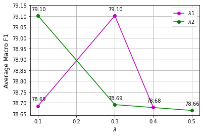


InfoDCL Training Hyper-Parameters.
For hyper-parameter tuning of our proposed InfoDCL framework, we randomly sample M tweets from the training set of our TweetEmoji-EN. We continue training the pre-trained RoBERTa for three epochs with Adam optimizer with a weight decay of and a peak learning rate of . The batch size is , and the total number of input samples is after constructing positive pairs. As Gao et al. 2021 find contrastive learning is not sensitive to the learning rate nor batch size when further training a PLM, we do not fine-tune these (i.e., the learning rate and batch size) in this paper. Following Liu et al. 2019, we mask of tokens for our MLM objective. We fine-tune the loss scaling weights in a set of , in a set of , and in a set of . To reduce search space, we use the same temperature value for the in Eq. 3 and Eq. 4 and fine-tune in a set of . We use grid search to find the best hyper-parameter set and evaluate performance on the Dev set of the English language Twitter datasets (excluding SentiThel). 2626 26 We fine-tune the learned model on each downstream task with an arbitrary learning rate of , a batch size of , and a training epoch of . The performance is macro- over three runs with random seeds. We select the best hyper-parameter set that achieves the best macro- averaged over the downstream tasks. Our best hyper-parameter set is , , , and . As Figure 4 shows, our model is not sensitive to changes of these hyper-parameters, and we observe that all the differences are less than comparing to the best hyper-parameter set. Finally, we continue training RoBERTa/BERTweet on the full training set of TweetEmoji-EN with InfoDCL framework and best hyper-parameters. We train InfoDCL model for three epochs and utilize Nvidia A100 GPU (GB each) and CPU cores. Each epoch takes around hours.
Downstream Task Fine-Tuning Hyper-Parameters.
Furthermore, we take the model trained with the best hyper-parameters and search the best hyper-parameter set of downstream task fine-tuning. We search the batch size in a set of and the peak learning rate in a set of . We identify the best fine-tuning hyper-parameters based on the macro- 2727 27 We run three times and use the mean of them. on Dev sets averaged over the English language Twitter datasets. Our best hyper-parameters for fine-tuning is a learning rate of and a batch size of . For all the downstream task fine-tuning experiments in this paper, we train a model on the task for epochs with early stop ( epochs). We use the same hyper-parameters identified in this full data setting for our few-shot learning. For each dataset, we fine-tune for five times with a different random seed every time, and report the mean macro- of the five runs. Each downstream fine-tuning experiment use a single Nvidia A100 GPU (GB) and CPU cores.
Baseline Hyper-Parameters.
Our Baseline (1) is directly fine-tuning RoBERTa on downstream tasks. We fine-tune Baseline (1) hyper-parameters as follows: The batch size is chosen from a set of and the peak learning rate in a set of . The best hyper-parameters for RoBERTa fine-tuning is a learning rate of and a batch size of .
For Baseline (2-3), we further pre-train the RoBERTa model for three epochs (same as our InfoDCL) with the MLM objective with an arbitrary learning rate of and a batch size of . We mask of tokens in each input tweet. For Baseline (3), we give priority to masking emojis in a tweet: if the emoji tokens are less than , we then randomly select regular tokens to complete the percentage of masking to the . Baseline (4) is about surrogate label prediction (with emojis). We also train Baseline (4) for three epochs with a learning rate of and a batch size of . After training, models are fine-tuned on downstream tasks using the same hyper-parameters as our proposed model.
Baselines (5-7). SimCSE Gao et al. 2021 was trained in two setups, i.e., self-supervised and supervised by label data. We also train RoBERTa on both settings. For self-supervised SimCSE, we train RoBERTa on our pre-training dataset for three epochs with a learning rate of , a batch size of , and of . For the distantly-supervised SimCSE, we construct positive pairs as described in Section B.4. Similar to self-supervised SimCSE, we train RoBERTa for three epochs with a learning rate of but with a batch size of . 2828 28 After pairing, each batch include unique tweets. The pre-training of Mirror-BERT is similar to the pre-training of self-supervised SimCSE. We set the span masking rate of , a temperature of , a learning rate of , and a batch size of . Trained models, then, are fine-tuned on downstream tasks. For downstream task fine-tuning with baselines 2-7, we use the same hyper-parameters identified with InfoDCL downstream task fine-tuning.
Baselines (8-9). SCL Gunel et al. 2021 and LCL Suresh and Ong 2021 directly fine-tune on downstream tasks with cross-entropy loss. We reproduce these two methods on our evaluation tasks. For SCL, we follow Gunel et al. 2021 and fine-tune each task with a temperature of , a SCL scaling weighting of , and a learning rate of . For LCL, we fine-tune each task with a temperature of , a LCL scaling weighting of , and a learning rate of .
Baselines (10). We implement WCL Zheng et al. 2021 to continue train RoBERTa with our emoji dataset. We remove all emojis in the M tweets and encode tweets using the hidden state of ‘[CLS]’ token from the last layer of RoBERTa. The tweets are then clustered by k-means clustering algorithm.2929 29 We use mini-batch k-means clustering from scikit-learn Pedregosa et al. 2011. For hyper-parmeter tuning of WCL, we randomly sample M tweets from the training set of TweetEmoji-EN and train a model for three epochs with different hyper-parmeter sets. We search the number of clusters in a set of and temperature in a set of . To reduce the search space, we use the same temperature value for SSCL and SCL losses. We evaluate performance on the Dev set of the English language Twitter datasets 3030 30 We fine-tune the trained WCL model with a learning rate of and a batch size of . and find the best hyper-parameter set is and . We then train WCL on the TweetEmoji-EN dataset for three epochs with our best hyper-parameters and fine tune the model on downstream tasks with the same hyper-parameters identified for InfoDCL downstream fine-tuning.3131 31 For hashtag-based experiment, we use the same hyper-parameters.
Baseline (11). We fine-tune BERTweet with hyperparameters utilized in Nguyen et al. 2020 that are a fixed learning of and a batch size of .
| lr | batch | |||||
| InfoDCL PT (emoji) | 0.3 | 0.1 | 0.5 | 0.3 | 128 | |
| InfoDCL PT (hashtag) | 0.4 | 0.1 | 0.1 | 0.1 | 128 | |
| DCL PT (emoji) | - | - | 0.5 | 0.3 | 128 | |
| DCL PT (hashtag) | - | - | 0.1 | 0.1 | 128 | |
| Downstream FT | - | - | - | - | 32 | |
| RoBERTa FT | - | - | - | - | 64 | |
| MLM | - | - | - | - | 4,096 | |
| E-MLM | - | - | - | - | 4,096 | |
| SLP | - | - | - | - | 4,096 | |
| SimCSE-Self | - | - | - | 0.05 | 256 | |
| SimCSE-Distant | - | - | - | 0.05 | 128 | |
| Mirror-BERT | - | - | - | 0.04 | 256 | |
| SCL | - | - | - | 0.30 | 32 | |
| LCL | - | - | - | 0.30 | 32 | |
| WCL | - | - | - | 0.10 | 256 | |
| BERTweet FT | - | - | - | - | 32 |
Multi-Lingual Experiment Hyper-Parameters.
For multi-lingual experiments, we utilize the pre-trained XLM-RoBERTaBase model Conneau et al. 2020 as our initial checkpoint. We continue training XLM-R on multi-lingual tweets with our framework and the best hyperparameters identified for English. For the downstream fine-tuning, we use as same as the best hyperparameters identified for English tasks.
Hahstag Experiment Hyper-Parameters.
For the hashtag-based experiments presented in Section E.4, we use the same hyper-parameter optimization set up to find the best hyper-parameter set for hashtag-based models. The best hyper-parameter set for hashtag-based models is , , , and . We then use the same downstream fine-tuning hyper-parameters identified with emoji-based InfoDCL for downstream task.
Appendix E Results
E.1 Standard Deviation and Significance Tests
| Task | RB | MLM | E-MLM | SLP | Mir-B | Sim-Self | Sim-D | SCL | LCL | WCL | DCL | InfoDCL-R | BTw | InfoDCL-B | |
| CrisisOltea | 0.15 | 0.15 | 0.23 | 0.17 | 0.24 | 0.30 | 0.25 | 0.23 | 0.13 | 0.29 | 0.25 | 0.15 | 0.26 | 0.07 | |
| EmoMoham | 1.60 | 0.85 | 0.72 | 1.05 | 0.50 | 0.85 | 0.70 | 0.56 | 0.37 | 0.53 | 0.93 | 0.79 | 0.66 | 0.70 | |
| HateWas | 0.21 | 0.63 | 0.79 | 0.55 | 0.21 | 0.19 | 0.40 | 0.21 | 0.25 | 0.24 | 0.67 | 0.41 | 0.63 | 0.57 | |
| HateDav | 1.31 | 0.85 | 0.58 | 0.36 | 1.71 | 1.39 | 1.04 | 0.43 | 1.24 | 0.93 | 0.81 | 0.61 | 0.78 | 0.76 | |
| HateBas | 1.96 | 2.20 | 1.86 | 1.64 | 0.82 | 1.62 | 2.65 | 3.52 | 1.20 | 2.21 | 0.47 | 1.00 | 3.50 | 1.88 | |
| In-Domain | HumorMea | 0.47 | 0.38 | 0.65 | 0.38 | 0.38 | 0.87 | 0.59 | 0.65 | 0.66 | 0.73 | 0.19 | 0.62 | 0.15 | 0.48 |
| IronyHee-A | 1.30 | 1.06 | 0.85 | 1.02 | 1.11 | 0.87 | 1.35 | 1.13 | 0.95 | 1.46 | 1.38 | 1.51 | 1.38 | 0.85 | |
| IronyHee-B | 1.60 | 0.63 | 2.43 | 2.38 | 0.56 | 0.84 | 2.70 | 2.03 | 1.44 | 0.89 | 1.05 | 0.53 | 2.06 | 3.19 | |
| OffenseZamp | 1.41 | 0.37 | 0.78 | 0.50 | 1.32 | 1.67 | 0.60 | 0.83 | 0.15 | 0.42 | 0.85 | 1.51 | 1.96 | 0.92 | |
| SarcRiloff | 1.47 | 1.34 | 2.58 | 1.26 | 4.32 | 2.06 | 1.86 | 2.79 | 2.03 | 1.15 | 0.85 | 1.09 | 1.69 | 1.60 | |
| SarcPtacek | 0.30 | 0.10 | 0.10 | 0.22 | 0.18 | 0.28 | 0.21 | 0.23 | 0.14 | 0.17 | 0.12 | 0.07 | 0.23 | 0.10 | |
| SarcRajad | 0.51 | 0.30 | 0.30 | 0.71 | 0.57 | 0.27 | 0.22 | 0.55 | 0.55 | 0.58 | 0.47 | 0.49 | 0.73 | 0.64 | |
| SarcBam | 0.54 | 0.61 | 0.87 | 0.38 | 0.69 | 1.18 | 0.60 | 0.83 | 0.78 | 0.36 | 0.48 | 0.39 | 0.31 | 0.71 | |
| SentiRosen | 0.93 | 1.64 | 0.35 | 0.91 | 1.06 | 0.57 | 0.67 | 1.14 | 0.40 | 0.73 | 0.76 | 0.52 | 0.40 | 0.43 | |
| SentiThel | 0.61 | 1.01 | 0.69 | 0.33 | 0.65 | 0.50 | 0.56 | 1.29 | 0.85 | 0.54 | 0.78 | 0.62 | 0.63 | 0.66 | |
| StanceMoham | 0.87 | 1.55 | 0.80 | 1.07 | 1.40 | 1.94 | 1.67 | 1.01 | 1.66 | 1.11 | 1.25 | 1.33 | 1.35 | 1.37 | |
| Average | 0.24 | 0.24 | 0.20 | 0.26 | 0.23 | 0.17 | 0.31 | 0.35 | 0.42 | 0.23 | 0.24 | 0.19 | 0.33 | 0.20 | |
| EmotionWall | 0.41 | 0.78 | 0.69 | 1.01 | 1.14 | 0.40 | 0.33 | 0.73 | 0.36 | 0.73 | 1.13 | 0.26 | 1.50 | 0.85 | |
| Out-of-Domain | EmotionDem | 0.58 | 0.60 | 0.42 | 0.80 | 0.71 | 0.88 | 0.74 | 0.52 | 1.05 | 0.86 | 1.28 | 0.61 | 1.20 | 1.73 |
| SarcWalk | 1.29 | 1.14 | 0.99 | 0.98 | 1.25 | 4.09 | 1.01 | 0.88 | 1.19 | 0.59 | 1.66 | 1.11 | 0.69 | 0.72 | |
| SarcOra | 1.20 | 1.41 | 0.99 | 0.24 | 1.56 | 1.85 | 0.32 | 1.33 | 1.70 | 1.21 | 0.68 | 0.77 | 1.05 | 1.00 | |
| Senti-MR | 0.56 | 0.29 | 0.70 | 0.50 | 0.32 | 0.27 | 0.27 | 0.46 | 0.41 | 0.61 | 0.30 | 0.39 | 0.57 | 0.43 | |
| Senti-YT | 0.52 | 0.59 | 0.43 | 0.36 | 1.00 | 0.95 | 0.37 | 0.37 | 0.62 | 0.29 | 0.53 | 0.26 | 0.25 | 0.52 | |
| SST-5 | 0.35 | 0.56 | 0.64 | 1.18 | 0.72 | 0.55 | 0.57 | 1.06 | 0.78 | 0.79 | 0.97 | 0.64 | 0.90 | 0.53 | |
| SST-2 | 0.39 | 0.41 | 0.40 | 0.22 | 0.38 | 0.35 | 0.50 | 0.34 | 0.30 | 0.35 | 0.32 | 0.24 | 0.32 | 0.22 | |
| Average | 0.31 | 0.15 | 0.27 | 0.41 | 0.19 | 0.42 | 0.21 | 0.26 | 0.17 | 0.14 | 0.54 | 0.27 | 0.28 | 0.12 |
| -value (t-test) | Minimal Distance (ASO) | |||
| In-Domain | Out-of-Domain | In-Domain | Out-of-Domain | |
| InfoDCL-RoBERTa vs. | ||||
| RoBERTa | 0.0000 | 0.0075 | 0.0000 | 0.0000 |
| MLM | 0.0002 | 0.0020 | 0.0000 | 0.0000 |
| E-MLM | 0.0100 | 0.0410 | 0.0000 | 0.0000 |
| SLP | 0.0213 | 0.0843 | 0.0000 | 0.0011 |
| Mirror-B | 0.0000 | 0.0001 | 0.0000 | 0.0000 |
| SimSCE-self | 0.0000 | 0.0000 | 0.0000 | 0.0000 |
| SimCSE-D | 0.0818 | 0.0005 | 0.0000 | 0.0000 |
| SCL | 0.0003 | 0.0014 | 0.0000 | 0.0000 |
| LCL | 0.0003 | 0.0001 | 0.0000 | 0.0000 |
| WCL | 0.0001 | 0.0001 | 0.0000 | 0.0000 |
| BERTweet | 0.0960 | 0.0000 | 0.0000 | 0.0000 |
| InfoDCL-BERTweet vs. | ||||
| BERTweet | 0.0076 | 0.0377 | 0.0321 | 0.0000 |
Table 10 shows the standard deviations of our emoji-based InfoDCl models and all baselines over five runs. We conduct two significance tests on our results, i.e., the classical paired student’s t-test Fisher 1936 and Almost Stochastic Order (ASO) Dror et al. 2019 (better adapts to results of neural networks). As we pointed out earlier, we run each experiment five times with different random seeds. Hence, we conduct these two significance tests by inputting the obtained five evaluation scores on the Test set. Table 11 presents -values for t-test and minimal distance at significance level of for ASO test. We also conduct significance tests on the results of individual tasks, finding that our InfoDCL-RoBERTa significantly () improves the original RoBERTa on (out of ) and (out of ) datasets based on t-test and ASO, respectively. InfoDCL-RoBERTa also significantly () outperforms BERTweet (the strongest baseline) on (out of ) and (out of ) tasks based on t-test and ASO, respectively.
E.2 Comparisons to Individual SoTAs.
Although the focus of our work is on producing effective representations suited to the whole class of SM tasks, rather than to one or another of these tasks, we also compare our models on each dataset to other reported task-specific SoTA models on that particular dataset in Table 12. We compare our methods on each dataset to other reported task-specific SoTA models on that particular dataset as shown. Due to diverse metrics used in previous studies, we compare models of each task reporting the corresponding metric of the SoTA method. Some SoTA models are trained on different data splits or use different evaluation approaches (e.g., Olteanu et al. 2014 is evaluated by cross-validation). To provide meaningful comparisons, we thus fine-tune BERTweet on our splits and report against our models. Our InfoDCL-RoBERTa outperform SoTA on out of in-domain datasets and four out of eight out-of-domain datasets. We achieve the best average score over in-domain datasets applying our model on BERTweet. Further training RoBERTa with our framework obtains the best average score across the eight out-of-domain datasets. We note that some SoTA models adopt task-specific approaches and/or require task-specific resources. For example, Ke et al. 2020 utilize SentiWordNet to identify the sentiment polarity of each word. In this work, our focus on producing effective representations suited for the whole class of SM tasks, rather than one or another of these tasks. Otherwise, we hypothesize that task-specific approaches can be combined with our InfoDCL framework to yield even better performance on individual tasks.
| Task | Metric | SoTA | BTw |
|
| |||||
| CrisisOltea | M- | 95.60 | 95.76 | 96.01 | 95.84 | |||||
| EmoMoham | M- | 78.50 | 80.23 | 81.34 | 81.96 | |||||
| HateWas | W- | 73.62 | 88.95 | 88.73 | 89.12 | |||||
| HateDav | W- | 90.00 | 91.26 | 91.12 | 91.27 | |||||
| HateBas | M- | 65.10 | 53.62 | 52.84 | 53.95 | |||||
| In-Domain | HumorMea | M- | 98.54 | 94.43 | 93.75 | 94.04 | ||||
| IronyHee-A | 70.50 | 73.99 | 72.10 | 74.81 | ||||||
| IronyHee-B | M- | 50.70 | 56.73 | 57.22 | 59.15 | |||||
| OffenseZamp | M- | 82.90 | 79.35 | 81.21 | 79.83 | |||||
| SarcRiloff | 51.00 | 66.59 | 65.90 | 69.28 | ||||||
| SarcPtacek | M- | 92.37 | 96.40 | 96.10 | 96.67 | |||||
| SarcRajad | Acc | 92.94 | 95.30 | 95.20 | 95.32 | |||||
| SarcBam | Acc | 85.10 | 81.79 | 81.51 | 83.22 | |||||
| SentiRosen | M-Rec | 72.60 | 72.91 | 72.77 | 72.46 | |||||
| SentiThel | Acc | 88.00 | 89.81 | 91.81 | 90.67 | |||||
| StanceMoham | Avg(a,f) | 71.00 | 71.26 | 73.31 | 72.09 | |||||
| Average | - | 78.65 | 80.52 | 80.68 | 81.23 | |||||
| EmotionWall | M- | 57.00 | 64.48 | 68.41 | 65.61 | |||||
| Out-of-Domain | EmotionDem | W- | 64.80 | 64.53 | 65.16 | 64.80 | ||||
| SarcWalk | M- | 69.00 | 67.27 | 68.45 | 67.30 | |||||
| SarcOra | M- | 75.00 | 77.33 | 77.41 | 76.88 | |||||
| Senti-MR | Acc | 90.82 | 87.95 | 89.43 | 88.21 | |||||
| Senti-YT | Acc | 93.00 | 93.24 | 93.12 | 93.47 | |||||
| SST-5 | Acc | 58.59 | 56.32 | 57.74 | 57.23 | |||||
| SST-2 | Acc | 96.70 | 93.32 | 94.98 | 93.73 | |||||
| Average | - | 75.61 | 75.55 | 76.84 | 75.90 |
| L | Task | XLM | InfoDCL-XLMR | SoTA | ||
| EN | Mono | Mult | ||||
| AR | EmoMag | 72.23 | 72.08 | 72.59 | 72.56 | 60.32 |
| IronyGhan | 81.15 | 78.75 | 81.85 | 82.23 | 84.40 | |
| OffenseMub | 84.87 | 85.08 | 85.61 | 87.10 | 90.50 | |
| IT | EmoBian | 70.37 | 73.51 | 73.58 | 74.36 | 71.00 |
| IronyCig | 73.22 | 73.52 | 74.07 | 73.42 | 73.10 | |
| HateBos | 78.63 | 78.06 | 79.44 | 79.77 | 79.93 | |
| ES | Emo-esMoham | 76.61 | 76.59 | 77.29 | 77.66 | — |
| IronyOrt | 72.88 | 73.11 | 72.98 | 74.91 | 71.67 | |
| Hate-esBas | 76.07 | 75.33 | 76.33 | 77.03 | 73.00 | |
| Average | 76.23 | 76.23 | 77.08 | 77.67 | — | |
| Task | RB | MLM | H-MLM | SLP | Mir-B | Sim-S | Sim-D | WCL | DCL | InfoD-R | BTw | InfoD-B | |
| CrisisOltea | 95.87 | 95.75 | 95.74 | 95.96 | 96.12 | 95.88 | 95.94 | 95.84 | 95.92 | 95.94 | 95.76 | 95.84 | |
| EmoMoham | 78.76 | 79.17 | 79.70 | 78.85 | 78.67 | 77.58 | 80.55 | 77.33 | 80.36 | 80.58 | 80.23 | 80.22 | |
| HateWas | 57.01 | 57.70 | 57.22 | 57.55 | 56.78 | 56.40 | 56.40 | 57.59 | 57.17 | 56.64 | 57.32 | 57.11 | |
| HateDav | 76.04 | 76.81 | 77.59 | 77.40 | 76.71 | 75.81 | 76.75 | 76.82 | 77.44 | 77.17 | 76.93 | 78.31 | |
| HateBas | 47.85 | 50.28 | 50.96 | 49.11 | 46.26 | 45.90 | 50.22 | 48.04 | 48.93 | 49.99 | 53.62 | 53.75 | |
| In-Domain | HumorMea | 93.28 | 93.30 | 93.46 | 93.55 | 92.21 | 91.81 | 94.07 | 92.51 | 94.64 | 93.88 | 94.43 | 94.25 |
| IronyHee-A | 72.87 | 73.05 | 73.68 | 73.87 | 71.64 | 69.76 | 77.41 | 72.88 | 76.41 | 75.94 | 77.03 | 79.51 | |
| IronyHee-B | 53.20 | 51.12 | 54.75 | 54.76 | 50.70 | 48.68 | 55.38 | 51.84 | 57.36 | 55.74 | 56.73 | 58.78 | |
| OffenseZamp | 79.93 | 79.81 | 79.20 | 80.74 | 79.73 | 79.74 | 80.56 | 79.53 | 80.55 | 80.65 | 79.35 | 79.36 | |
| SarcRiloff | 73.71 | 70.04 | 72.44 | 74.12 | 68.73 | 67.92 | 75.22 | 70.51 | 75.90 | 74.51 | 78.76 | 78.83 | |
| SarcPtacek | 95.99 | 95.99 | 96.15 | 95.99 | 95.57 | 95.20 | 96.07 | 95.68 | 96.19 | 95.98 | 96.40 | 96.66 | |
| SarcRajad | 85.21 | 85.97 | 85.79 | 85.72 | 84.60 | 83.93 | 86.71 | 85.61 | 86.76 | 86.77 | 87.13 | 87.43 | |
| SarcBam | 79.79 | 80.32 | 80.84 | 80.09 | 78.95 | 78.31 | 81.45 | 79.79 | 81.24 | 80.33 | 81.76 | 83.87 | |
| SentiRosen | 89.55 | 89.59 | 90.20 | 89.05 | 87.33 | 85.58 | 90.35 | 88.34 | 90.76 | 90.93 | 89.53 | 89.59 | |
| SentiThel | 71.41 | 72.19 | 71.72 | 71.81 | 71.12 | 70.66 | 72.19 | 71.63 | 71.71 | 71.93 | 71.64 | 71.82 | |
| StanceMoham | 69.44 | 69.95 | 70.34 | 69.77 | 65.47 | 64.76 | 70.16 | 68.80 | 70.87 | 70.73 | 68.33 | 67.30 | |
| Average | 76.24 | 76.31 | 76.86 | 76.77 | 75.04 | 74.25 | 77.46 | 75.80 | 77.64 | 77.36 | 77.81 | 78.29 | |
| EmotionWall | 66.51 | 66.41 | 67.34 | 65.27 | 63.92 | 62.19 | 68.37 | 63.45 | 67.78 | 67.74 | 64.48 | 64.64 | |
| Out-of-Domain | EmotionDem | 56.59 | 56.19 | 56.50 | 56.00 | 56.15 | 56.20 | 56.68 | 55.78 | 56.24 | 55.76 | 53.33 | 55.61 |
| SarcWalk | 67.50 | 67.90 | 68.66 | 65.06 | 63.65 | 66.15 | 67.48 | 66.87 | 66.53 | 68.44 | 67.27 | 67.86 | |
| SarcOra | 76.92 | 77.41 | 76.06 | 76.85 | 75.37 | 76.34 | 76.82 | 76.44 | 77.38 | 77.77 | 77.33 | 77.04 | |
| Senti-MR | 89.00 | 89.90 | 89.48 | 88.96 | 88.86 | 88.73 | 90.29 | 88.94 | 90.14 | 90.12 | 87.94 | 88.06 | |
| Senti-YT | 90.22 | 90.65 | 90.40 | 90.19 | 89.59 | 87.74 | 91.81 | 90.44 | 91.68 | 92.16 | 92.25 | 92.65 | |
| SST-5 | 54.96 | 55.92 | 55.52 | 55.69 | 55.00 | 54.35 | 56.26 | 54.18 | 55.40 | 56.33 | 55.74 | 55.97 | |
| SST-2 | 94.57 | 94.69 | 94.34 | 94.39 | 93.76 | 93.07 | 94.14 | 94.12 | 94.42 | 95.15 | 93.32 | 93.72 | |
| Average | 74.53 | 74.88 | 74.79 | 74.05 | 73.29 | 73.10 | 75.23 | 73.78 | 74.94 | 75.43 | 73.96 | 74.44 |
E.3 Multilingual Tasks
We also investigate the effectiveness of our proposed model on multilingual tasks. Table 13 shows the performance on nine downstream tasks in three different languages. Here, we continue training XLM-R with our proposed objectives. We experiment with three settings: (1) English only: training on the TweetEmoji-1M and evaluating on the nine multilingual datasets, (2) Target mono-lingual: training on each M mono-lingual tweets in the target language independently (i.e., TweetEmoji-AR for Arabic, TweetEmoji-IT for Italian, and TweetEmoji-ES for Spanish) and evaluating on the respective dataset corresponding to the same language as training data, and (3) Multilingual: training on the TweetEmoji-Multi dataset and evaluating on the nine multilingual datasets. We still use the NPMI weighting matrix generated from English tweets in these experiments. 3232 32 We plan to explore generating the NPMI weighting matrix from mutlilingual data in future work. Table 13 shows that our models outperform the original XLM-R on all the datasets and obtains improvements of and average across the nine datasets under the multilingual and target mono-lingual settings, respectively. Training on English mono-lingual data helps four datasets, but cannot benefit all the nine non-English datasets on average. Compared to previous SoTA models, our proposed methods outperform these on six out of nine datasets. 3333 33 For Emo-esMoham, we use fine-tuning XLM-R as SoTA model because we convert the intensity regression task to a emotion classification and there is no SoTA model. These results demonstrate that our methods are not only task-agnostic within the realm of SM tasks, but also language-independent.
E.4 Using Hashtag as Distant Supervision
As Table 14 presents, our proposed framework also can enhance the representation quality using hashtags as distantly supervised labels. InfoDCL-RoBERTa, the model further training RoBERTa on the training set of TweetHashtag-EN with our framework, obtains average of and across the in-domain and eight out-of-domain datasets, respectively. Comapred to baselines, our DCL obtains the best performance average score across in-domain datasets ( ). InfoDCL-BERTweet, the further pre-trained BERTweet on the training set of TweetHashtag-EN with our framework, obtains average of and across the in-domain and eight out-of-domain datasets, respectively.
E.5 Topic Classification
We fine-tune baselines and our models on two topic classification datasets and report macro scores in Table 15. We find that our hashtag-based InfoDCL model acquires best performance on both datasets, for AGNews , and for TopicDao . These results indicate that our framework can also effectively improve topic classification when we use hashtags as distant labels.
| Emoji-based | Hashtag-based | ||||||
| Model | AGN | Topic | Ave | Model | AGN | Topic | Ave |
| RB | 96.97 | 94.75 | 95.86 | - | - | - | - |
| MLM | 97.00 | 94.58 | 95.79 | MLM | 97.01 | 94.78 | 95.89 |
| E-MLM | 96.97 | 94.73 | 95.85 | E-MLM | 97.13 | 94.66 | 95.90 |
| SLP | 97.12 | 94.54 | 95.83 | SLP | 97.04 | 94.63 | 95.84 |
| Mir-B | 96.86 | 94.72 | 95.79 | Mir-B | 97.13 | 94.66 | 95.90 |
| Sim-S | 96.88 | 94.73 | 95.81 | Sim-S | 96.90 | 94.65 | 95.78 |
| Sim-D | 97.08 | 94.70 | 95.89 | Sim-D | 97.30 | 94.79 | 96.04 |
| WCL | 97.13 | 94.65 | 95.89 | WCL | 97.09 | 94.56 | 95.83 |
| DCL | 97.08 | 94.59 | 95.84 | DCL | 97.23 | 94.64 | 95.93 |
| InfoD-R | 97.01 | 94.48 | 95.74 | InfoD-R | 97.42 | 94.80 | 96.11 |
| BTw | 97.00 | 94.43 | 95.72 | - | - | - | - |
| InfoD-B | 97.05 | 94.47 | 95.76 | InfoD-B | 97.26 | 94.49 | 95.87 |
| Task | RB | MLM | E-MLM | SLP | Mir-B | Sim-S | Sim-D | WCL | DCL | InfoD-R | BTw | InfoD-B |
| STS12 | 15.88 | 37.71 | 34.55 | 50.07 | 59.07 | 54.18 | 46.13 | 34.81 | 46.46 | 48.13 | 29.20 | 42.54 |
| STS13 | 38.11 | 55.72 | 53.90 | 53.87 | 69.89 | 65.06 | 45.99 | 37.56 | 47.24 | 51.44 | 36.26 | 44.40 |
| STS14 | 28.58 | 40.16 | 40.86 | 44.88 | 63.82 | 59.18 | 43.20 | 24.51 | 42.76 | 46.79 | 33.76 | 38.95 |
| STS15 | 40.22 | 59.49 | 56.35 | 61.83 | 73.78 | 70.30 | 52.76 | 50.36 | 49.11 | 58.04 | 49.19 | 54.67 |
| STS16 | 50.12 | 62.13 | 65.12 | 58.41 | 74.20 | 70.45 | 51.17 | 36.33 | 45.39 | 57.09 | 46.99 | 49.42 |
| SICK-R | 62.54 | 64.42 | 63.48 | 64.21 | 64.29 | 63.53 | 57.14 | 47.22 | 56.93 | 62.81 | 48.76 | 59.15 |
| STS-B | 46.63 | 56.00 | 58.50 | 59.93 | 68.75 | 64.49 | 53.00 | 42.24 | 50.64 | 56.65 | 38.24 | 52.46 |
| Average | 40.30 | 53.66 | 53.25 | 56.17 | 67.69 | 63.88 | 49.91 | 39.00 | 48.36 | 54.42 | 40.34 | 48.80 |
| MR | 75.92 | 76.85 | 80.62 | 86.79 | 76.72 | 73.77 | 86.04 | 78.96 | 86.83 | 86.66 | 79.58 | 86.12 |
| CR | 69.59 | 77.35 | 84.79 | 89.69 | 81.48 | 80.19 | 89.48 | 83.74 | 90.36 | 89.75 | 80.82 | 89.62 |
| SUBJ | 91.50 | 90.63 | 91.01 | 92.24 | 91.57 | 90.29 | 91.24 | 92.91 | 92.61 | 93.71 | 93.03 | 93.53 |
| MPQA | 73.75 | 80.40 | 78.54 | 87.93 | 85.39 | 83.92 | 87.18 | 85.30 | 87.51 | 87.12 | 71.78 | 86.21 |
| SST2 | 82.81 | 85.50 | 88.14 | 92.53 | 81.05 | 78.69 | 91.87 | 85.28 | 91.43 | 92.59 | 86.66 | 91.10 |
| SST5 | 38.46 | 41.81 | 46.65 | 52.31 | 44.48 | 41.45 | 48.60 | 43.48 | 50.77 | 53.08 | 43.71 | 52.13 |
| TREC | 61.40 | 73.20 | 72.20 | 78.60 | 87.00 | 86.00 | 74.60 | 84.20 | 75.80 | 83.00 | 80.80 | 83.40 |
| MRPC | 71.42 | 73.04 | 74.09 | 74.61 | 74.67 | 74.49 | 71.59 | 71.88 | 71.54 | 73.22 | 72.35 | 72.00 |
| Average | 70.61 | 74.85 | 77.01 | 81.84 | 77.80 | 76.10 | 80.08 | 78.22 | 80.86 | 82.39 | 76.09 | 81.76 |
E.6 SentEval
Each STS dataset includes pairs of sentences each with a gold semantic similarity score ranging from to . We encode each sentence by the hidden state of ‘[CLS]’ token from the last Transformer encoder layer. We then calculate the Spearman’s correlation between cosine similarity of sentence embeddings and the gold similarity score of each pair. Same as Mirror-BERT Liu et al. 2021a and SimCSE Gao et al. 2021, we report the overall Spearman’s correlation. For transfer learning tasks, we follow the evaluation protocal of SentEval, where a trainable logistic regression classifier is added on top of a frozen encoder that is an PLM. We report classification accuracy of eight transfer learning datasets in Tables 16. Although our InfoDCL underperforms Mirror-BERT on all STS datasets, but it still outperforms than Baseline 1, 2, and 3. Our InfoDCL is not designed to improve STS task but it does not hurt performance compared to Baseline 2. Moreover, our InfoDCL achieves the best average performance on eight transferring datasets. We note that four datasets are SM tasks. Only regarding the other four non-SM tasks, our InfoDCL model still outperforms most baselines and achieves the second best performance on average, which is only points lower than Mirror-BERT.


E.7 Few Shot Learning
Since InfoDCL exploits an extensive set of cues in the data that capture a broad range of fine-grained SM concepts, we hypothesize it will be also effective in few-shot learning. Hence, we test this hypothesis for both in-domain and out-of-domain tasks. Figure 5 and Table 19 compare our models to three strong baselines when they are trained with different percentages of training samples. Results show that our proposed InfoDCL model always outperforms all baselines on average scores across both in-domain and out-of-domain tasks. For in-domain tasks, our InfoDCL-RoBERTa remarkably surpasses the RoBERTa baseline with a sizable average scores when we only provide training data from downstream tasks. Compared to other strong baselines, fine-tuning BERTweet and SimCSE-Distant (also our method), InfoDCL-RoBERTa outperforms these with and average scores, respectively, when we use training data for downstream fine-tuning. With only of gold data, InfoDCL-RoBERTa improves points over the RoBERTa baseline. For eight out-of-domain tasks, InfoDCL-RoBERTa outperforms the RoBERTa, BERTweet, and SimCSE-Distant baselines with , , and average scores, respectively, when the models are only fine-tuned on training data of downstream tasks. As Figure 5(b) and Table 19 show, InfoDCL-RoBERTa consistently outperforms all the baselines given any percentage of training data. Tables 20, 21, 22, 23, 24, and 25, respectively, present the performance of RoBERTa, BERTweet, SimCSE-Distant, DCL, InfoDCL-RoBERTa, InfoDCL-BERTweet on all our English downstream datasets and various few-shot settings.
Appendix F Analyses
F.1 Model Analysis
Table 17 shows that both PMI and EC-Emb are capable of capturing sensible correlations between emojis (although the embedding approach includes a few semantically distant emojis, such as the emoji ‘
’ being highly related to ‘
’).
| Q | Method | 1 | 2 | 3 | 4 | 5 | 6 | 7 | 8 | 9 | 10 | ||||||||||||||||||||
|
|
PMI |
|
|
|
|
|
|
|
|
|
| ||||||||||||||||||||
| E-em |
|
|
|
|
|
|
|
|
|
| |||||||||||||||||||||
![[Uncaptioned image]](2203.07648v5/emojis/1f1e9-1f1ea.png)
|
PMI |
|
|
|
|
|
|
|
|
|
| ||||||||||||||||||||
| E-em |
|
|
|
|
|
|
|
|
|
| |||||||||||||||||||||
![[Uncaptioned image]](2203.07648v5/emojis/1f328-fe0f.png)
|
PMI |
|
|
|
|
|
|
|
|
|
| ||||||||||||||||||||
| E-em |
|
|
|
|
|
|
|
|
|
|
![[Uncaptioned image]](2203.07648v5/emojis/1f60a.png)
![[Uncaptioned image]](2203.07648v5/emojis/1f603.png)
![[Uncaptioned image]](2203.07648v5/emojis/1f44d.png)
![[Uncaptioned image]](2203.07648v5/emojis/1f38a.png)
![[Uncaptioned image]](2203.07648v5/emojis/1f389.png)
![[Uncaptioned image]](2203.07648v5/emojis/1f61d.png)
![[Uncaptioned image]](2203.07648v5/emojis/1f61c.png)
![[Uncaptioned image]](2203.07648v5/emojis/1f381.png)
![[Uncaptioned image]](2203.07648v5/emojis/1f62c.png)
![[Uncaptioned image]](2203.07648v5/emojis/1f602.png)
![[Uncaptioned image]](2203.07648v5/emojis/1f605.png)
![[Uncaptioned image]](2203.07648v5/emojis/1f60c.png)
![[Uncaptioned image]](2203.07648v5/emojis/1f1e8-1f1f3.png)
![[Uncaptioned image]](2203.07648v5/emojis/1f1f7-1f1fa.png)
![[Uncaptioned image]](2203.07648v5/emojis/1f1f0-1f1f7.png)
![[Uncaptioned image]](2203.07648v5/emojis/1f1ea-1f1f8.png)
![[Uncaptioned image]](2203.07648v5/emojis/1f1eb-1f1f7.png)
![[Uncaptioned image]](2203.07648v5/emojis/1f1ef-1f1f5.png)
![[Uncaptioned image]](2203.07648v5/emojis/1f1ee-1f1f9.png)
![[Uncaptioned image]](2203.07648v5/emojis/1f1ec-1f1e7.png)
![[Uncaptioned image]](2203.07648v5/emojis/1f1f5-1f1f9.png)
![[Uncaptioned image]](2203.07648v5/emojis/1f1e6-1f1fa.png)
![[Uncaptioned image]](2203.07648v5/emojis/1f1ee-1f1ea.png)
![[Uncaptioned image]](2203.07648v5/emojis/2618-fe0f.png)
![[Uncaptioned image]](2203.07648v5/emojis/26f3.png)
![[Uncaptioned image]](2203.07648v5/emojis/1f3d2.png)
![[Uncaptioned image]](2203.07648v5/emojis/1f1f5-1f1f0.png)
![[Uncaptioned image]](2203.07648v5/emojis/1f1f5-1f1ed.png)
![[Uncaptioned image]](2203.07648v5/emojis/26c4.png)
![[Uncaptioned image]](2203.07648v5/emojis/1f32c-fe0f.png)
![[Uncaptioned image]](2203.07648v5/emojis/2744-fe0f.png)
![[Uncaptioned image]](2203.07648v5/emojis/1f326-fe0f.png)
![[Uncaptioned image]](2203.07648v5/emojis/1f329-fe0f.png)
![[Uncaptioned image]](2203.07648v5/emojis/1f32b-fe0f.png)
![[Uncaptioned image]](2203.07648v5/emojis/1f327-fe0f.png)
![[Uncaptioned image]](2203.07648v5/emojis/1f325-fe0f.png)
![[Uncaptioned image]](2203.07648v5/emojis/26c8-fe0f.png)
![[Uncaptioned image]](2203.07648v5/emojis/1f32a-fe0f.png)
![[Uncaptioned image]](2203.07648v5/emojis/1f301.png)
![[Uncaptioned image]](2203.07648v5/emojis/1f681.png)
![[Uncaptioned image]](2203.07648v5/emojis/1f302.png)
![[Uncaptioned image]](2203.07648v5/emojis/1f3d6-fe0f.png)
![[Uncaptioned image]](2203.07648v5/emojis/1f68c.png)
F.2 Qualitative Analysis
We provide a qualitative visualization analysis of our model representation. For this purpose, we use our InfoDCL-RoBERTa to obtain representations of samples in the TweetEmoji-EN’s validation set (‘[CLS]’ token from the last encoder layer) then average the representations of all tweets with the same surrogate label (emoji). We then project these emoji embeddings into a two-dimensional space using -SNE. As Fig. 6 shows, we can observe a number of distinguishable clusters. For instance, a cluster of love and marriage is grouped in the left region, unhappy and angry faces are in the right side, and food at the bottom. We can also observe sensible relations between clusters. For instance, the cluster of love and marriage is close to the cluster of smiling faces but is far away from the cluster of unhappy faces. In addition, the cluster of aquatic animals (middle bottom) is close to terrestrial animals while each of these is still visually distinguishable. We also note that emojis which contain the same emoji character but differ in skin tone are clustered together. An example of these is emojis of Santa Claus (left bottom). This indicates that our InfoDCL model has meticulously captured the relations between the emoji surrogate labels.

Appendix G Uniformity and Tolerance
Wang and Liu 2021 investigate representation quality measuring the uniformity of an embedding distribution and the tolerance to semantically similar samples. Given a dataset and an encoder , the uniformity is based on a gaussian potential kernel introduced by Wang and Isola 2020 and is formulated as:
| (11) |
where . Wang and Liu 2021 use as the uniformity metric, thus a higher uniformity score indicates that the embedding distribution is closer to a uniform distribution.
The tolerance metric measures the mean of similarities of samples belonging to the same class, which defined as:
| (12) |
where is the supervised label of sample . is an indicator function, giving the value of for and the value of for . In our experiments, we use gold development samples from our downstream SM datasets.
| Task | InfoDCL | A | B | C | D | E | F | G | H | I |
| CrisisOltea | 96.01 | 95.91 | 95.88 | 95.91 | 95.83 | 95.96 | 95.92 | 95.75 | 95.96 | 95.79 |
| EmoMoham | 81.34 | 82.31 | 82.03 | 80.98 | 80.06 | 81.28 | 80.54 | 81.27 | 82.11 | 81.49 |
| HateWas | 57.30 | 57.13 | 57.09 | 57.03 | 57.30 | 57.24 | 57.14 | 56.89 | 57.08 | 57.12 |
| HateDav | 77.29 | 76.82 | 77.88 | 77.59 | 76.74 | 76.11 | 76.79 | 77.69 | 77.40 | 77.15 |
| HateBas | 52.84 | 51.77 | 52.39 | 51.90 | 52.79 | 51.26 | 52.17 | 51.67 | 53.63 | 50.97 |
| HumorMea | 93.75 | 93.08 | 93.62 | 93.17 | 94.23 | 93.64 | 94.13 | 93.26 | 93.87 | 93.78 |
| IronyHee-A | 76.31 | 76.41 | 77.14 | 77.11 | 74.99 | 78.19 | 77.15 | 76.95 | 76.55 | 76.18 |
| IronyHee-B | 57.22 | 55.88 | 57.60 | 56.01 | 53.98 | 58.69 | 57.48 | 56.51 | 57.62 | 56.00 |
| OffenseZamp | 81.21 | 80.49 | 81.13 | 80.97 | 80.45 | 79.01 | 79.94 | 81.05 | 80.40 | 81.61 |
| SarcRiloff | 78.31 | 76.26 | 76.78 | 77.44 | 74.81 | 78.09 | 79.26 | 77.76 | 78.22 | 76.14 |
| SarcPtacek | 96.10 | 95.96 | 95.85 | 96.18 | 95.84 | 96.45 | 96.13 | 95.94 | 96.10 | 96.20 |
| SarcRajad | 87.00 | 86.54 | 86.63 | 86.69 | 86.79 | 87.61 | 87.45 | 86.85 | 86.66 | 86.63 |
| SarcBam | 81.49 | 81.35 | 81.74 | 81.34 | 80.82 | 83.02 | 81.31 | 81.69 | 81.80 | 81.46 |
| SentiRosen | 91.59 | 91.51 | 91.62 | 91.91 | 91.51 | 91.44 | 90.65 | 91.97 | 91.28 | 91.85 |
| SentiThel | 71.87 | 71.65 | 71.60 | 71.67 | 72.09 | 71.19 | 71.73 | 72.01 | 71.50 | 71.80 |
| StanceMoham | 71.13 | 71.03 | 70.51 | 71.84 | 69.75 | 70.80 | 69.74 | 70.66 | 70.35 | 70.45 |
| Average | 78.17 | 77.75 | 78.09 | 77.98 | 77.37 | 78.12 | 77.97 | 78.00 | 78.16 | 77.79 |
| Percentage | 1 | 5 | 10 | 20 | 30 | 40 | 50 | 60 | 70 | 80 | 90 | 100 |
| In-Domain | ||||||||||||
| RoBERTa | 46.96 | 62.70 | 66.41 | 71.96 | 73.54 | 74.34 | 75.09 | 74.99 | 75.37 | 75.95 | 76.27 | 76.24 |
| BERTweet | 46.87 | 60.46 | 64.75 | 69.08 | 74.96 | 75.88 | 76.35 | 76.70 | 77.12 | 77.39 | 77.92 | 77.81 |
| Sim-D | 56.23 | 65.43 | 70.19 | 73.70 | 75.24 | 75.45 | 76.08 | 76.32 | 76.79 | 77.01 | 77.35 | 77.81 |
| DCL | 59.05 | 67.12 | 71.81 | 74.33 | 75.45 | 75.85 | 76.47 | 76.80 | 77.17 | 77.29 | 77.54 | 77.97 |
| InfoDCL-RB | 59.78 | 68.45 | 73.19 | 74.85 | 75.82 | 75.98 | 76.81 | 76.93 | 77.37 | 77.35 | 77.67 | 78.17 |
| InfoDCL-BTw | 56.06 | 65.54 | 70.24 | 74.54 | 75.84 | 76.10 | 76.68 | 76.99 | 77.42 | 77.77 | 78.11 | 78.58 |
| Out-of-Domain | ||||||||||||
| RoBERTa | 32.62 | 50.10 | 52.38 | 67.80 | 71.41 | 72.64 | 73.44 | 73.89 | 74.16 | 74.13 | 74.53 | 74.53 |
| BERTweet | 33.33 | 48.69 | 52.01 | 58.68 | 62.52 | 69.81 | 70.67 | 71.74 | 72.32 | 73.08 | 73.48 | 73.96 |
| Sim-D | 45.96 | 55.74 | 61.32 | 69.05 | 70.74 | 72.01 | 72.80 | 73.03 | 73.94 | 74.22 | 74.36 | 74.48 |
| DCL | 49.72 | 59.60 | 65.35 | 69.64 | 71.76 | 72.79 | 73.44 | 73.59 | 74.26 | 74.36 | 74.71 | 75.37 |
| InfoDCL-RB | 48.85 | 62.06 | 67.10 | 70.75 | 72.28 | 73.45 | 74.17 | 74.44 | 74.95 | 75.22 | 75.28 | 75.54 |
| InfoDCL-BTw | 45.59 | 54.15 | 59.42 | 67.43 | 70.61 | 71.50 | 72.33 | 72.50 | 73.12 | 73.63 | 74.15 | 74.32 |
| Percentage | # of Training Samples | |||||||||||||||
| 1 | 5 | 10 | 20 | 30 | 40 | 50 | 60 | 70 | 80 | 90 | 100 | 20 | 100 | 500 | 1000 | |
| CrisisOltea | 94.88 | 95.18 | 95.59 | 95.67 | 95.73 | 95.65 | 95.88 | 95.77 | 95.72 | 95.83 | 95.92 | 95.87 | 37.20 | 70.27 | 95.09 | 95.20 |
| EmoMoham | 13.39 | 51.63 | 70.83 | 74.20 | 75.45 | 76.42 | 76.59 | 76.70 | 78.00 | 77.85 | 77.40 | 78.76 | 14.21 | 14.68 | 73.85 | 75.49 |
| HateWas | 28.23 | 52.72 | 54.66 | 55.30 | 56.65 | 58.78 | 56.80 | 56.77 | 56.64 | 57.26 | 59.98 | 57.01 | 26.59 | 32.94 | 52.98 | 54.53 |
| HateDav | 38.02 | 71.66 | 73.50 | 74.74 | 76.08 | 76.55 | 76.06 | 77.31 | 77.62 | 76.58 | 77.65 | 76.04 | 30.64 | 30.47 | 67.68 | 71.24 |
| HateBas | 44.61 | 51.48 | 48.71 | 48.77 | 48.29 | 45.60 | 48.60 | 46.46 | 47.72 | 50.35 | 46.78 | 47.85 | 41.43 | 42.54 | 49.49 | 46.99 |
| HumorMea | 38.08 | 88.33 | 90.07 | 91.33 | 91.33 | 92.08 | 92.00 | 91.92 | 92.34 | 92.75 | 92.17 | 93.28 | 42.28 | 58.71 | 90.08 | 91.20 |
| IronyHee-A | 41.78 | 56.76 | 64.98 | 68.11 | 68.82 | 69.62 | 70.68 | 71.67 | 70.66 | 72.92 | 73.44 | 72.87 | 44.79 | 55.90 | 65.82 | 68.05 |
| IronyHee-B | 20.49 | 34.16 | 41.95 | 46.54 | 48.62 | 48.10 | 51.49 | 51.29 | 51.20 | 52.25 | 53.22 | 53.20 | 20.29 | 21.98 | 44.58 | 47.52 |
| OffenseZamp | 42.70 | 75.61 | 77.99 | 77.70 | 79.24 | 79.04 | 79.60 | 79.81 | 78.83 | 80.73 | 80.45 | 79.93 | 34.63 | 41.89 | 76.09 | 76.90 |
| SarcRiloff | 45.76 | 44.48 | 43.99 | 53.03 | 65.37 | 71.90 | 73.46 | 70.35 | 71.81 | 73.72 | 74.29 | 73.71 | 45.65 | 43.99 | 70.53 | 74.78 |
| SarcPtacek | 81.99 | 85.98 | 87.24 | 88.72 | 89.99 | 91.15 | 92.01 | 92.73 | 93.51 | 94.16 | 95.07 | 95.99 | 45.05 | 39.78 | 81.35 | 83.21 |
| SarcRajad | 69.83 | 76.95 | 79.45 | 81.02 | 82.07 | 82.34 | 83.48 | 83.36 | 84.29 | 84.19 | 85.21 | 85.21 | 47.42 | 47.01 | 64.09 | 73.27 |
| SarcBam | 62.09 | 73.41 | 75.41 | 76.39 | 77.15 | 77.46 | 78.50 | 78.92 | 79.39 | 78.79 | 79.59 | 79.79 | 43.90 | 61.87 | 73.11 | 75.10 |
| SentiRosen | 40.91 | 43.05 | 36.98 | 86.94 | 87.53 | 88.73 | 88.49 | 88.95 | 89.61 | 88.82 | 89.66 | 89.55 | 45.27 | 57.00 | 88.78 | 89.55 |
| SentiThel | 65.13 | 68.73 | 69.87 | 69.56 | 70.02 | 71.06 | 70.69 | 70.96 | 70.22 | 70.83 | 70.76 | 71.41 | 19.46 | 24.10 | 65.52 | 67.15 |
| StanceMoham | 23.45 | 33.07 | 51.42 | 63.28 | 64.34 | 65.02 | 67.21 | 66.87 | 68.36 | 68.21 | 68.73 | 69.44 | 24.70 | 27.57 | 61.95 | 65.05 |
| Average | 46.96 | 62.70 | 66.41 | 71.96 | 73.54 | 74.34 | 75.09 | 74.99 | 75.37 | 75.95 | 76.27 | 76.24 | 35.22 | 41.92 | 70.06 | 72.20 |
| EmotionWall | 5.54 | 7.10 | 10.44 | 41.46 | 57.69 | 61.02 | 62.59 | 64.16 | 65.74 | 64.83 | 65.76 | 66.51 | 4.19 | 21.06 | 63.93 | 66.50 |
| EmotionDem | 12.73 | 42.06 | 46.31 | 51.58 | 52.65 | 53.90 | 54.89 | 54.58 | 55.67 | 55.49 | 56.28 | 56.59 | 0.51 | 2.47 | 30.70 | 41.68 |
| SarcWalk | 40.08 | 34.73 | 43.92 | 62.89 | 63.02 | 66.13 | 66.64 | 67.67 | 67.43 | 67.69 | 68.96 | 67.50 | 35.22 | 51.67 | 67.02 | 67.39 |
| SarcOra | 45.66 | 53.56 | 48.87 | 74.78 | 75.47 | 75.19 | 76.55 | 77.27 | 77.02 | 77.40 | 77.07 | 76.92 | 45.92 | 63.66 | 77.69 | 75.42 |
| Senti-MR | 44.08 | 85.93 | 87.02 | 87.98 | 88.52 | 88.30 | 89.13 | 88.84 | 89.29 | 89.31 | 89.05 | 89.00 | 40.69 | 67.17 | 86.02 | 87.17 |
| Senti-YT | 40.90 | 40.48 | 40.49 | 78.67 | 88.28 | 90.19 | 89.47 | 90.29 | 89.42 | 89.59 | 89.86 | 90.22 | 45.05 | 43.40 | 89.55 | 90.24 |
| SST-5 | 8.87 | 45.89 | 50.01 | 52.26 | 52.57 | 53.37 | 54.00 | 54.51 | 54.94 | 54.81 | 54.79 | 54.96 | 10.91 | 11.70 | 47.76 | 50.42 |
| SST-2 | 63.12 | 91.09 | 91.99 | 92.75 | 93.11 | 93.05 | 94.28 | 93.78 | 93.74 | 93.89 | 94.49 | 94.57 | 34.08 | 67.80 | 91.44 | 92.50 |
| Average | 32.62 | 50.10 | 52.38 | 67.80 | 71.41 | 72.64 | 73.44 | 73.89 | 74.16 | 74.13 | 74.53 | 74.53 | 27.07 | 41.12 | 69.26 | 71.42 |
| Percentage | # of Training Samples | |||||||||||||||
| 1 | 5 | 10 | 20 | 30 | 40 | 50 | 60 | 70 | 80 | 90 | 100 | 20 | 100 | 500 | 1000 | |
| CrisisOltea | 93.47 | 95.07 | 95.42 | 95.40 | 95.53 | 95.55 | 95.59 | 95.79 | 95.63 | 95.76 | 95.68 | 95.76 | 50.00 | 46.96 | 94.65 | 95.02 |
| EmoMoham | 20.49 | 18.15 | 53.35 | 73.16 | 76.84 | 76.95 | 78.00 | 78.55 | 78.88 | 79.54 | 79.94 | 80.23 | 20.02 | 16.86 | 70.70 | 75.59 |
| HateWas | 28.22 | 51.43 | 53.03 | 54.95 | 55.62 | 55.54 | 56.26 | 56.46 | 56.39 | 56.26 | 56.91 | 57.32 | 29.25 | 28.22 | 51.29 | 53.60 |
| HateDav | 28.86 | 68.38 | 73.29 | 75.37 | 76.60 | 76.12 | 77.32 | 76.39 | 76.77 | 77.07 | 76.90 | 76.93 | 31.20 | 30.34 | 57.32 | 67.51 |
| HateBas | 50.93 | 54.01 | 52.50 | 53.49 | 53.56 | 53.77 | 52.72 | 53.69 | 54.42 | 54.98 | 53.51 | 53.62 | 45.40 | 46.97 | 51.86 | 54.08 |
| HumorMea | 42.89 | 90.08 | 92.22 | 92.98 | 93.13 | 93.56 | 93.57 | 93.82 | 94.00 | 93.90 | 94.33 | 94.43 | 45.11 | 44.00 | 90.90 | 92.15 |
| IronyHee-A | 46.60 | 56.60 | 67.13 | 72.41 | 74.13 | 74.43 | 76.25 | 76.26 | 76.39 | 77.06 | 78.15 | 77.03 | 47.26 | 55.23 | 71.80 | 75.48 |
| IronyHee-B | 19.99 | 21.82 | 30.42 | 39.89 | 46.99 | 47.97 | 49.80 | 51.11 | 53.21 | 54.25 | 56.66 | 56.73 | 17.08 | 21.35 | 33.09 | 45.62 |
| OffenseZamp | 44.58 | 73.92 | 76.19 | 78.03 | 79.25 | 79.58 | 79.10 | 79.65 | 79.40 | 79.60 | 80.32 | 79.35 | 45.86 | 45.30 | 74.47 | 75.95 |
| SarcRiloff | 44.49 | 44.19 | 45.48 | 43.99 | 78.47 | 78.96 | 78.14 | 78.29 | 79.28 | 78.93 | 79.67 | 78.76 | 45.77 | 44.92 | 77.83 | 78.66 |
| SarcPtacek | 85.44 | 88.13 | 89.21 | 90.71 | 91.61 | 92.47 | 93.34 | 93.77 | 94.39 | 95.03 | 95.76 | 96.40 | 53.31 | 43.61 | 83.95 | 86.01 |
| SarcRajad | 47.01 | 82.25 | 82.89 | 84.70 | 85.09 | 85.70 | 85.87 | 86.52 | 86.32 | 86.87 | 86.65 | 87.13 | 47.90 | 47.01 | 47.01 | 80.09 |
| SarcBam | 62.12 | 76.58 | 78.45 | 79.24 | 80.48 | 81.26 | 81.32 | 81.61 | 81.64 | 81.93 | 82.05 | 81.76 | 45.48 | 42.21 | 76.34 | 77.86 |
| SentiRosen | 45.50 | 50.05 | 41.24 | 42.27 | 78.93 | 87.63 | 88.36 | 88.70 | 89.20 | 89.35 | 89.76 | 89.53 | 51.81 | 52.98 | 88.86 | 89.82 |
| SentiThel | 61.79 | 68.00 | 70.32 | 70.70 | 71.35 | 71.85 | 71.77 | 71.64 | 71.51 | 71.95 | 72.44 | 71.64 | 24.59 | 19.20 | 63.77 | 66.84 |
| StanceMoham | 27.59 | 28.67 | 34.79 | 58.06 | 61.74 | 62.71 | 64.13 | 64.86 | 66.43 | 65.74 | 68.01 | 68.33 | 26.19 | 26.47 | 59.82 | 61.65 |
| Average | 46.87 | 60.46 | 64.75 | 69.08 | 74.96 | 75.88 | 76.35 | 76.70 | 77.12 | 77.39 | 77.92 | 77.81 | 39.14 | 38.23 | 68.35 | 73.50 |
| EmotionWall | 8.44 | 8.78 | 7.76 | 17.85 | 31.73 | 45.72 | 51.85 | 56.03 | 58.17 | 61.24 | 62.31 | 64.48 | 6.25 | 7.86 | 55.09 | 62.94 |
| EmotionDem | 1.74 | 22.10 | 33.95 | 43.88 | 46.79 | 47.76 | 49.06 | 49.61 | 51.02 | 51.24 | 52.89 | 53.33 | 1.27 | 1.48 | 4.41 | 20.92 |
| SarcWalk | 44.46 | 49.15 | 52.05 | 60.70 | 64.68 | 65.06 | 65.05 | 66.16 | 66.17 | 67.48 | 67.57 | 67.27 | 49.57 | 53.74 | 65.94 | 69.24 |
| SarcOra | 48.93 | 59.61 | 57.33 | 75.14 | 75.32 | 76.06 | 75.06 | 76.70 | 76.04 | 77.04 | 76.73 | 77.33 | 40.55 | 64.86 | 76.03 | 76.76 |
| Senti-MR | 48.58 | 84.79 | 86.21 | 86.57 | 87.36 | 87.98 | 87.77 | 87.25 | 88.02 | 88.05 | 88.13 | 87.94 | 43.58 | 59.23 | 85.45 | 86.68 |
| Senti-YT | 48.07 | 46.96 | 42.87 | 43.43 | 50.78 | 90.74 | 91.20 | 91.77 | 91.94 | 92.05 | 91.93 | 92.25 | 45.43 | 44.56 | 91.75 | 91.91 |
| SST-5 | 14.15 | 28.93 | 45.48 | 50.25 | 51.58 | 52.82 | 52.79 | 53.32 | 54.24 | 54.26 | 54.87 | 55.74 | 14.34 | 12.86 | 32.28 | 46.22 |
| SST-2 | 52.28 | 89.19 | 90.43 | 91.63 | 91.96 | 92.31 | 92.55 | 93.04 | 92.91 | 93.28 | 93.44 | 93.32 | 46.12 | 70.62 | 89.23 | 91.08 |
| Average | 33.33 | 48.69 | 52.01 | 58.68 | 62.52 | 69.81 | 70.67 | 71.74 | 72.32 | 73.08 | 73.48 | 73.96 | 30.89 | 39.40 | 62.52 | 68.22 |
| Percentage | # of Training Samples | |||||||||||||||
| 1 | 5 | 10 | 20 | 30 | 40 | 50 | 60 | 70 | 80 | 90 | 100 | 20 | 100 | 500 | 1000 | |
| CrisisOltea | 94.21 | 94.94 | 95.28 | 95.53 | 95.69 | 95.72 | 95.76 | 95.81 | 95.89 | 95.96 | 95.86 | 95.94 | 61.80 | 90.88 | 94.31 | 94.63 |
| EmoMoham | 24.31 | 53.06 | 75.65 | 77.15 | 78.46 | 78.53 | 78.77 | 79.68 | 80.17 | 79.75 | 81.00 | 81.05 | 23.47 | 41.68 | 76.72 | 78.35 |
| HateWas | 32.05 | 51.26 | 53.38 | 54.94 | 55.47 | 56.18 | 55.99 | 56.46 | 56.80 | 57.06 | 57.29 | 57.13 | 34.03 | 32.73 | 51.66 | 53.03 |
| HateDav | 38.33 | 71.56 | 73.83 | 74.42 | 76.12 | 75.36 | 76.50 | 76.98 | 76.96 | 75.93 | 77.81 | 77.15 | 34.57 | 34.33 | 66.42 | 70.04 |
| HateBas | 52.43 | 49.63 | 48.54 | 49.62 | 50.11 | 48.63 | 50.51 | 49.55 | 50.98 | 52.33 | 51.20 | 52.32 | 48.50 | 48.69 | 47.91 | 47.77 |
| HumorMea | 87.85 | 91.21 | 92.17 | 92.34 | 92.86 | 92.70 | 92.98 | 92.72 | 93.39 | 93.83 | 93.45 | 93.42 | 61.12 | 89.40 | 92.11 | 92.33 |
| IronyHee-A | 55.34 | 65.12 | 69.03 | 70.36 | 71.15 | 72.07 | 72.34 | 72.80 | 74.06 | 73.86 | 75.32 | 75.36 | 47.78 | 62.27 | 69.17 | 70.81 |
| IronyHee-B | 24.70 | 29.93 | 38.35 | 46.56 | 48.07 | 49.36 | 51.92 | 52.88 | 53.28 | 53.24 | 53.02 | 54.06 | 22.69 | 28.97 | 43.97 | 47.44 |
| OffenseZamp | 56.44 | 75.83 | 76.51 | 78.26 | 79.01 | 79.86 | 80.08 | 79.38 | 80.17 | 79.91 | 80.31 | 80.80 | 50.05 | 47.84 | 74.67 | 77.01 |
| SarcRiloff | 49.67 | 50.08 | 50.87 | 69.15 | 76.39 | 75.52 | 76.36 | 76.03 | 76.45 | 77.53 | 78.14 | 80.27 | 49.37 | 48.90 | 74.22 | 77.77 |
| SarcPtacek | 84.26 | 87.25 | 88.17 | 89.49 | 90.47 | 91.68 | 92.41 | 93.16 | 93.89 | 94.56 | 95.35 | 96.07 | 62.61 | 64.88 | 83.56 | 84.73 |
| SarcRajad | 80.89 | 83.20 | 83.92 | 85.12 | 85.78 | 85.21 | 86.01 | 86.18 | 86.14 | 86.19 | 86.24 | 87.20 | 48.68 | 48.28 | 80.20 | 82.51 |
| SarcBam | 70.06 | 75.35 | 77.85 | 78.05 | 79.21 | 79.65 | 79.83 | 80.64 | 80.60 | 81.69 | 81.23 | 81.40 | 53.37 | 65.46 | 74.84 | 76.49 |
| SentiRosen | 50.91 | 60.45 | 76.82 | 87.28 | 89.19 | 89.62 | 89.81 | 89.84 | 90.01 | 90.34 | 90.13 | 90.64 | 62.69 | 85.07 | 90.69 | 90.31 |
| SentiThel | 63.40 | 68.90 | 70.07 | 70.03 | 70.96 | 71.30 | 71.15 | 71.13 | 71.17 | 71.17 | 71.56 | 71.68 | 26.96 | 35.60 | 64.63 | 66.59 |
| StanceMoham | 34.85 | 39.11 | 52.68 | 60.98 | 64.86 | 65.87 | 66.81 | 67.96 | 68.71 | 68.80 | 69.71 | 70.48 | 32.19 | 39.92 | 59.86 | 64.41 |
| Average | 56.23 | 65.43 | 70.19 | 73.70 | 75.24 | 75.45 | 76.08 | 76.32 | 76.79 | 77.01 | 77.35 | 77.81 | 44.99 | 54.06 | 71.56 | 73.39 |
| EmotionWall | 11.47 | 23.74 | 33.53 | 47.89 | 56.53 | 61.85 | 63.77 | 64.81 | 66.67 | 66.60 | 67.51 | 67.68 | 13.27 | 37.34 | 64.42 | 67.28 |
| EmotionDem | 6.54 | 32.45 | 43.01 | 47.14 | 48.98 | 50.07 | 52.00 | 52.55 | 54.19 | 55.42 | 55.41 | 55.27 | 1.41 | 5.04 | 16.61 | 30.48 |
| SarcWalk | 49.94 | 51.42 | 54.93 | 61.15 | 60.60 | 62.37 | 62.92 | 62.95 | 63.91 | 64.63 | 64.12 | 65.04 | 51.43 | 53.00 | 63.73 | 65.99 |
| SarcOra | 53.84 | 63.83 | 65.38 | 73.30 | 75.02 | 75.14 | 76.09 | 75.99 | 77.31 | 77.61 | 77.44 | 77.12 | 47.54 | 69.24 | 73.89 | 77.37 |
| Senti-MR | 83.37 | 86.80 | 87.12 | 87.29 | 87.68 | 87.76 | 88.23 | 87.98 | 88.45 | 88.66 | 88.45 | 89.09 | 58.39 | 84.19 | 86.24 | 87.12 |
| Senti-YT | 52.25 | 53.93 | 63.56 | 90.35 | 90.83 | 91.66 | 91.65 | 91.61 | 92.11 | 92.17 | 92.24 | 92.23 | 55.59 | 74.67 | 91.96 | 92.03 |
| SST-5 | 22.17 | 42.07 | 51.01 | 52.34 | 53.02 | 53.87 | 54.06 | 54.38 | 54.98 | 54.85 | 55.46 | 55.09 | 16.13 | 17.87 | 46.35 | 50.77 |
| SST-2 | 88.13 | 91.65 | 92.01 | 92.97 | 93.27 | 93.36 | 93.69 | 93.92 | 93.91 | 93.84 | 94.22 | 94.29 | 68.44 | 90.28 | 91.63 | 92.95 |
| Average | 45.96 | 55.74 | 61.32 | 69.05 | 70.74 | 72.01 | 72.80 | 73.03 | 73.94 | 74.22 | 74.36 | 74.48 | 39.02 | 53.95 | 66.85 | 70.50 |
| Percentage | # of Training Samples | |||||||||||||||
| 1 | 5 | 10 | 20 | 30 | 40 | 50 | 60 | 70 | 80 | 90 | 100 | 20 | 100 | 500 | 1000 | |
| CrisisOltea | 94.25 | 94.97 | 95.33 | 95.49 | 95.55 | 95.66 | 95.75 | 95.81 | 95.85 | 95.92 | 95.82 | 95.92 | 54.77 | 90.26 | 94.09 | 94.89 |
| EmoMoham | 40.74 | 64.88 | 74.52 | 75.24 | 78.39 | 77.92 | 77.96 | 79.74 | 79.67 | 79.42 | 80.54 | 80.54 | 33.70 | 52.43 | 77.18 | 77.97 |
| HateWas | 32.38 | 51.72 | 53.62 | 54.54 | 55.74 | 56.05 | 56.38 | 56.78 | 56.92 | 57.00 | 56.95 | 57.14 | 32.73 | 37.08 | 51.77 | 52.93 |
| HateDav | 51.88 | 70.75 | 72.86 | 76.27 | 76.30 | 75.80 | 76.30 | 76.45 | 77.00 | 75.89 | 76.79 | 76.79 | 32.33 | 34.89 | 67.12 | 69.86 |
| HateBas | 47.58 | 48.71 | 46.41 | 50.88 | 48.70 | 48.72 | 49.00 | 48.70 | 49.28 | 50.14 | 50.15 | 52.17 | 49.36 | 51.14 | 49.74 | 50.93 |
| HumorMea | 89.39 | 91.94 | 92.07 | 92.95 | 93.53 | 93.06 | 93.52 | 93.29 | 93.64 | 93.99 | 94.05 | 94.13 | 66.98 | 90.18 | 91.98 | 92.32 |
| IronyHee-A | 58.60 | 63.36 | 69.51 | 71.60 | 73.16 | 73.97 | 75.39 | 76.02 | 76.41 | 76.56 | 76.56 | 77.15 | 56.24 | 63.66 | 70.44 | 73.55 |
| IronyHee-B | 30.15 | 35.38 | 39.40 | 47.69 | 49.89 | 51.10 | 53.27 | 53.96 | 55.58 | 54.95 | 56.19 | 57.48 | 24.25 | 30.94 | 44.08 | 49.57 |
| OffenseZamp | 58.21 | 76.41 | 76.68 | 78.07 | 78.99 | 79.24 | 79.38 | 80.28 | 79.95 | 79.82 | 79.67 | 79.94 | 53.99 | 47.43 | 74.20 | 76.37 |
| SarcRiloff | 48.09 | 53.79 | 73.04 | 75.10 | 77.06 | 78.67 | 79.46 | 78.18 | 78.00 | 78.63 | 79.12 | 79.26 | 51.01 | 66.24 | 77.01 | 79.09 |
| SarcPtacek | 84.03 | 86.98 | 88.38 | 89.79 | 90.68 | 91.65 | 92.24 | 93.01 | 93.93 | 94.72 | 95.45 | 96.13 | 61.84 | 77.55 | 83.80 | 85.23 |
| SarcRajad | 81.12 | 83.42 | 84.50 | 85.62 | 85.75 | 86.10 | 86.24 | 86.16 | 86.77 | 86.99 | 86.90 | 87.45 | 49.20 | 56.02 | 80.90 | 82.63 |
| SarcBam | 69.96 | 75.07 | 77.42 | 78.85 | 79.13 | 80.33 | 80.60 | 80.79 | 81.25 | 81.37 | 80.68 | 81.31 | 52.21 | 66.83 | 75.82 | 76.61 |
| SentiRosen | 63.33 | 65.42 | 85.20 | 87.69 | 88.39 | 89.09 | 89.49 | 90.43 | 90.16 | 90.71 | 90.49 | 90.65 | 60.24 | 84.45 | 90.35 | 90.59 |
| SentiThel | 62.19 | 68.26 | 69.31 | 70.54 | 71.70 | 71.25 | 71.29 | 71.17 | 71.82 | 71.56 | 71.07 | 71.73 | 35.47 | 44.11 | 63.57 | 65.76 |
| StanceMoham | 32.91 | 42.83 | 50.68 | 58.91 | 64.28 | 65.01 | 67.25 | 68.06 | 68.51 | 68.99 | 70.19 | 69.74 | 31.31 | 39.80 | 59.99 | 63.38 |
| Average | 59.05 | 67.12 | 71.81 | 74.33 | 75.45 | 75.85 | 76.47 | 76.80 | 77.17 | 77.29 | 77.54 | 77.97 | 46.60 | 58.31 | 72.00 | 73.86 |
| EmotionWall | 13.32 | 24.15 | 35.91 | 51.67 | 60.54 | 64.25 | 65.18 | 65.55 | 67.36 | 66.92 | 68.68 | 68.36 | 15.03 | 37.66 | 66.24 | 68.38 |
| EmotionDem | 9.07 | 34.76 | 44.44 | 48.15 | 49.17 | 51.96 | 53.83 | 53.82 | 55.36 | 55.50 | 54.97 | 57.43 | 2.49 | 6.95 | 18.31 | 31.65 |
| SarcWalk | 50.36 | 53.15 | 58.43 | 61.57 | 62.78 | 63.28 | 64.74 | 64.01 | 65.57 | 64.88 | 66.28 | 67.39 | 49.08 | 54.10 | 64.36 | 67.36 |
| SarcOra | 54.61 | 64.78 | 66.60 | 71.23 | 74.62 | 75.61 | 76.67 | 76.85 | 76.08 | 77.58 | 76.78 | 77.76 | 49.37 | 69.83 | 76.78 | 78.04 |
| Senti-MR | 84.79 | 86.30 | 86.80 | 87.80 | 87.57 | 87.55 | 87.93 | 87.61 | 88.60 | 88.58 | 88.92 | 89.15 | 61.15 | 85.41 | 86.48 | 86.93 |
| Senti-YT | 65.50 | 78.44 | 85.95 | 90.51 | 91.81 | 91.83 | 91.42 | 91.62 | 91.67 | 92.00 | 92.30 | 92.26 | 66.60 | 82.08 | 92.01 | 92.47 |
| SST-5 | 29.58 | 43.42 | 51.77 | 52.75 | 53.85 | 54.16 | 53.71 | 54.99 | 55.06 | 54.82 | 55.29 | 56.00 | 23.75 | 25.60 | 48.93 | 51.38 |
| SST-2 | 90.50 | 91.78 | 92.87 | 93.42 | 93.71 | 93.72 | 94.05 | 94.27 | 94.34 | 94.57 | 94.46 | 94.64 | 70.04 | 91.35 | 92.65 | 93.51 |
| Average | 49.72 | 59.60 | 65.35 | 69.64 | 71.76 | 72.79 | 73.44 | 73.59 | 74.26 | 74.36 | 74.71 | 75.37 | 42.19 | 56.62 | 68.22 | 71.21 |
| Percentage | # of Training Samples | |||||||||||||||
| 1 | 5 | 10 | 20 | 30 | 40 | 50 | 60 | 70 | 80 | 90 | 100 | 20 | 100 | 500 | 1000 | |
| CrisisOltea | 94.88 | 95.26 | 95.61 | 95.59 | 95.65 | 95.75 | 95.82 | 95.72 | 95.85 | 95.88 | 96.04 | 95.94 | 67.01 | 93.24 | 94.87 | 95.10 |
| EmoMoham | 30.07 | 66.09 | 76.41 | 77.93 | 79.08 | 78.51 | 79.80 | 80.42 | 80.69 | 79.35 | 80.96 | 81.05 | 23.74 | 55.31 | 77.21 | 79.26 |
| HateWas | 33.12 | 53.06 | 54.15 | 54.85 | 55.84 | 56.30 | 56.65 | 56.73 | 56.90 | 57.10 | 57.30 | 57.13 | 33.88 | 38.36 | 52.63 | 54.14 |
| HateDav | 62.43 | 72.62 | 74.77 | 74.38 | 75.47 | 76.11 | 77.32 | 77.53 | 77.19 | 77.08 | 77.96 | 77.15 | 33.47 | 42.19 | 68.00 | 70.83 |
| HateBas | 48.02 | 48.66 | 48.78 | 52.54 | 51.48 | 50.25 | 53.48 | 52.29 | 52.31 | 52.70 | 53.59 | 52.32 | 52.09 | 50.49 | 48.85 | 52.44 |
| HumorMea | 88.09 | 90.52 | 91.37 | 92.07 | 92.55 | 92.20 | 92.34 | 92.02 | 92.25 | 92.61 | 92.06 | 93.42 | 58.63 | 89.43 | 91.06 | 91.55 |
| IronyHee-A | 62.51 | 67.18 | 70.63 | 72.21 | 72.78 | 73.84 | 74.06 | 74.57 | 76.09 | 77.13 | 76.26 | 75.36 | 53.15 | 65.05 | 70.91 | 73.73 |
| IronyHee-B | 28.46 | 35.86 | 43.12 | 48.50 | 50.67 | 51.71 | 52.75 | 54.00 | 54.99 | 54.55 | 55.01 | 54.06 | 28.56 | 32.75 | 46.88 | 50.10 |
| OffenseZamp | 66.53 | 76.15 | 78.21 | 79.30 | 79.49 | 80.23 | 80.56 | 80.20 | 80.93 | 80.39 | 80.55 | 80.80 | 51.41 | 51.08 | 75.55 | 77.78 |
| SarcRiloff | 53.31 | 54.58 | 74.38 | 73.01 | 75.32 | 74.26 | 76.59 | 75.62 | 76.76 | 76.63 | 77.33 | 80.27 | 52.42 | 64.76 | 76.90 | 76.52 |
| SarcPtacek | 84.69 | 87.39 | 88.36 | 89.73 | 90.54 | 91.25 | 92.40 | 93.07 | 93.88 | 94.57 | 95.29 | 96.07 | 66.07 | 77.98 | 83.83 | 85.59 |
| SarcRajad | 79.77 | 82.55 | 83.75 | 84.78 | 85.64 | 85.50 | 85.80 | 85.68 | 86.11 | 86.10 | 86.35 | 87.20 | 48.87 | 52.95 | 79.76 | 81.44 |
| SarcBam | 71.06 | 75.57 | 77.61 | 78.89 | 79.21 | 80.11 | 80.42 | 80.33 | 80.92 | 80.51 | 81.02 | 81.40 | 54.57 | 68.07 | 75.05 | 76.81 |
| SentiRosen | 54.63 | 73.04 | 86.34 | 89.20 | 90.11 | 90.67 | 90.36 | 91.14 | 91.24 | 91.23 | 91.36 | 90.64 | 69.13 | 88.21 | 91.31 | 91.38 |
| SentiThel | 65.10 | 69.63 | 70.46 | 70.68 | 71.74 | 71.83 | 72.02 | 71.77 | 71.85 | 72.10 | 71.57 | 71.68 | 25.34 | 39.56 | 65.87 | 67.34 |
| StanceMoham | 33.86 | 47.08 | 57.05 | 63.91 | 67.62 | 67.18 | 68.54 | 69.82 | 70.00 | 69.65 | 70.11 | 70.48 | 31.78 | 41.55 | 64.78 | 67.55 |
| Average | 59.78 | 68.45 | 73.19 | 74.85 | 75.82 | 75.98 | 76.81 | 76.93 | 77.37 | 77.35 | 77.67 | 77.81 | 46.88 | 59.44 | 72.72 | 74.47 |
| EmotionWall | 14.07 | 23.50 | 37.91 | 54.60 | 61.89 | 65.34 | 65.90 | 67.00 | 67.37 | 67.15 | 67.84 | 67.68 | 11.85 | 44.18 | 67.15 | 68.85 |
| EmotionDem | 13.43 | 39.26 | 45.52 | 48.55 | 50.46 | 51.77 | 54.37 | 54.93 | 55.58 | 56.87 | 57.31 | 55.27 | 2.66 | 6.23 | 24.99 | 38.03 |
| SarcWalk | 47.28 | 52.12 | 60.47 | 63.49 | 64.28 | 65.45 | 66.92 | 66.19 | 68.03 | 67.72 | 68.04 | 65.04 | 48.78 | 52.23 | 66.80 | 67.28 |
| SarcOra | 54.88 | 70.84 | 72.21 | 74.24 | 74.46 | 76.80 | 76.64 | 77.36 | 77.47 | 77.93 | 77.43 | 77.12 | 54.03 | 70.98 | 76.68 | 76.26 |
| Senti-MR | 84.62 | 85.83 | 87.25 | 87.74 | 88.52 | 88.47 | 89.11 | 88.82 | 89.63 | 89.60 | 89.30 | 89.09 | 50.89 | 85.00 | 85.77 | 86.91 |
| Senti-YT | 54.82 | 84.10 | 87.81 | 90.23 | 90.51 | 91.20 | 91.38 | 91.77 | 91.69 | 92.03 | 91.83 | 92.23 | 72.37 | 89.37 | 91.53 | 91.81 |
| SST-5 | 30.24 | 48.09 | 52.28 | 53.25 | 53.90 | 54.18 | 54.64 | 55.08 | 55.11 | 55.44 | 55.65 | 55.09 | 17.17 | 27.91 | 49.03 | 52.71 |
| SST-2 | 91.45 | 92.79 | 93.31 | 93.86 | 94.20 | 94.39 | 94.40 | 94.34 | 94.69 | 95.07 | 94.88 | 94.29 | 69.91 | 92.15 | 92.90 | 93.54 |
| Average | 48.85 | 62.06 | 67.10 | 70.75 | 72.28 | 73.45 | 74.17 | 74.44 | 74.95 | 75.22 | 75.28 | 74.48 | 40.96 | 58.51 | 69.36 | 71.92 |
| Percentage | # of Training Samples | |||||||||||||||
| 1 | 5 | 10 | 20 | 30 | 40 | 50 | 60 | 70 | 80 | 90 | 100 | 20 | 100 | 500 | 1000 | |
| CrisisOltea | 94.09 | 95.07 | 95.29 | 95.55 | 95.70 | 95.60 | 95.83 | 95.79 | 95.86 | 95.84 | 95.84 | 95.84 | 57.68 | 89.00 | 94.13 | 94.79 |
| EmoMoham | 29.53 | 34.42 | 67.80 | 74.42 | 77.04 | 77.55 | 77.83 | 79.56 | 80.06 | 80.66 | 80.04 | 81.96 | 25.21 | 30.90 | 73.64 | 76.25 |
| HateWas | 31.12 | 52.01 | 53.92 | 54.92 | 55.82 | 55.86 | 56.38 | 56.95 | 56.48 | 57.11 | 56.94 | 57.65 | 33.14 | 31.69 | 52.52 | 53.62 |
| HateDav | 32.42 | 69.28 | 74.02 | 75.12 | 76.59 | 76.15 | 76.77 | 77.05 | 77.23 | 77.40 | 77.77 | 77.94 | 32.84 | 31.47 | 60.75 | 68.86 |
| HateBas | 51.79 | 51.63 | 49.39 | 52.39 | 53.50 | 52.64 | 53.08 | 52.50 | 53.38 | 54.20 | 55.84 | 53.95 | 49.49 | 49.46 | 51.08 | 52.60 |
| HumorMea | 78.62 | 91.25 | 92.61 | 92.83 | 93.25 | 93.03 | 93.09 | 93.23 | 93.43 | 93.87 | 93.72 | 94.04 | 52.07 | 88.45 | 91.22 | 92.71 |
| IronyHee-A | 58.84 | 67.69 | 71.74 | 72.94 | 73.57 | 75.46 | 77.06 | 76.00 | 76.59 | 77.90 | 77.87 | 78.72 | 54.94 | 63.05 | 72.41 | 74.13 |
| IronyHee-B | 21.92 | 32.05 | 36.96 | 46.94 | 50.06 | 50.79 | 52.74 | 53.28 | 56.22 | 55.36 | 58.12 | 59.15 | 23.50 | 30.29 | 39.78 | 49.35 |
| OffenseZamp | 55.61 | 74.56 | 77.48 | 78.14 | 79.31 | 79.64 | 79.68 | 80.47 | 79.96 | 80.91 | 80.26 | 79.83 | 53.79 | 52.02 | 73.74 | 76.39 |
| SarcRiloff | 56.77 | 54.25 | 53.80 | 77.93 | 79.83 | 79.47 | 78.91 | 78.66 | 79.29 | 78.81 | 79.14 | 80.52 | 55.84 | 52.23 | 78.41 | 79.21 |
| SarcPtacek | 85.54 | 87.98 | 89.01 | 90.47 | 91.32 | 92.31 | 93.00 | 93.77 | 94.37 | 95.14 | 95.77 | 96.67 | 62.96 | 66.66 | 84.86 | 85.91 |
| SarcRajad | 80.56 | 82.99 | 83.82 | 84.98 | 86.12 | 86.07 | 86.12 | 86.34 | 86.10 | 86.78 | 86.42 | 87.20 | 48.97 | 48.55 | 80.24 | 81.42 |
| SarcBam | 71.96 | 78.74 | 79.64 | 81.03 | 80.94 | 81.84 | 82.25 | 81.96 | 82.42 | 82.88 | 83.11 | 83.20 | 54.47 | 67.95 | 77.88 | 79.86 |
| SentiRosen | 51.13 | 67.15 | 80.51 | 87.87 | 88.24 | 88.69 | 88.92 | 89.22 | 89.49 | 89.95 | 89.63 | 90.41 | 62.97 | 78.22 | 89.73 | 90.35 |
| SentiThel | 65.32 | 69.46 | 69.76 | 70.62 | 71.07 | 71.31 | 71.22 | 71.65 | 71.71 | 71.45 | 72.09 | 71.98 | 26.79 | 28.37 | 64.63 | 67.71 |
| StanceMoham | 31.67 | 40.06 | 48.05 | 56.54 | 61.17 | 61.10 | 64.04 | 65.38 | 66.12 | 66.08 | 67.19 | 68.22 | 29.90 | 33.94 | 55.87 | 61.30 |
| Average | 56.06 | 65.54 | 70.24 | 74.54 | 75.84 | 76.10 | 76.68 | 76.99 | 77.42 | 77.77 | 78.11 | 78.58 | 45.29 | 52.64 | 71.31 | 74.03 |
| EmotionWall | 12.31 | 14.81 | 27.45 | 44.30 | 54.18 | 57.67 | 60.11 | 59.24 | 62.41 | 64.31 | 65.20 | 65.61 | 13.00 | 29.74 | 61.28 | 65.57 |
| EmotionDem | 4.39 | 26.17 | 36.93 | 45.15 | 48.75 | 50.02 | 50.85 | 51.32 | 52.58 | 53.59 | 53.77 | 54.99 | 3.30 | 3.01 | 13.11 | 23.36 |
| SarcWalk | 47.12 | 50.30 | 54.64 | 56.70 | 62.89 | 62.29 | 64.76 | 65.53 | 65.84 | 65.57 | 67.73 | 67.30 | 46.91 | 51.50 | 65.01 | 67.89 |
| SarcOra | 49.18 | 66.42 | 68.51 | 70.98 | 74.05 | 74.78 | 75.17 | 75.85 | 75.40 | 76.33 | 77.27 | 76.88 | 49.69 | 67.78 | 76.81 | 76.70 |
| Senti-MR | 82.95 | 86.37 | 87.16 | 87.16 | 88.30 | 88.30 | 88.37 | 88.11 | 88.19 | 88.58 | 88.32 | 88.21 | 55.86 | 83.00 | 85.77 | 86.90 |
| Senti-YT | 56.44 | 59.69 | 59.46 | 90.81 | 91.02 | 92.04 | 92.13 | 92.06 | 92.35 | 92.23 | 92.36 | 92.41 | 64.98 | 44.15 | 92.22 | 92.07 |
| SST-5 | 23.14 | 38.42 | 49.67 | 52.45 | 52.98 | 54.06 | 54.09 | 54.45 | 54.84 | 55.01 | 55.13 | 55.93 | 17.84 | 21.24 | 40.02 | 49.84 |
| SST-2 | 89.22 | 91.04 | 91.52 | 91.85 | 92.72 | 92.84 | 93.16 | 93.45 | 93.33 | 93.44 | 93.42 | 93.73 | 58.17 | 90.51 | 90.88 | 91.69 |
| Average | 45.59 | 54.15 | 59.42 | 67.43 | 70.61 | 71.50 | 72.33 | 72.50 | 73.12 | 73.63 | 74.15 | 74.38 | 38.72 | 48.87 | 65.64 | 69.25 |