Let ${\bf x}_{t}$ with components $x_{it}$ be a vector of asset values with $i=1,\ldots,N$ in an investment universe of $N$ assets at the beginning of the period $[t,t+\Delta t]$, where $t$ is the current time and $\Delta t$ is a time step size. Let us start with a discrete-time asset price dynamics in the presence of outside investors described by the following equations:

	$\displaystyle{\bf x}_{t+\Delta t}=(1+{\bf r}_{t}\Delta t)\circ({\bf x}_{t}+{\bf a}_{t}\circ{\bf x}_{t}\Delta t),$
	$\displaystyle{\bf r}_{t}=r+{\bf w}{\bf z}_{t}+{\bf f}({\bf a}_{t})+\frac{1}{\sqrt{\Delta t}}\text{\boldmath$\varepsilon$}_{t},$		(2)

where $\circ$ stands for the element-wise product. Here the first equation in (2.1) defines the change of asset values in the time step $[t,t+\Delta t]$ as a composition of two changes to their time-$t$ values ${\bf x}_{t}$. First, at the beginning of the interval, investors adjust positions in each stock $i$ by buying (or selling, depending on the sign of $a_{it}$) the amount $a_{it}x_{it}\Delta t$ of the stock (so that the action vector ${\bf a}_{t}$ is defined as an instantaneous rate of change with the dimension of inverse time). Therefore, immediately after that the asset value is deterministically changed to ${\bf x}_{t}^{+}:={\bf x}_{t}+{\bf a}_{t}\circ{\bf x}_{t}\Delta t$. After that, the new portfolio ${\bf x}_{t}^{+}={\bf x}_{t}+{\bf a}_{t}\circ{\bf x}_{t}\Delta t$ grows at rate ${\bf r}_{t+\Delta t}$. The latter is given by the second of Eqs.(2.1) that defines the vector of equity returns as a combination of a risk-free rate $r$, predictors ${\bf z}_{t}$ with weights ${\bf w}$, a multivariate noise $\text{\boldmath$\varepsilon$}_{t}\sim\mathcal{N}(\cdot|{\bf 0},{\bf\Sigma})$, and a vector-valued market impact factor ${\bf f}({\bf a}_{t})$ with components $f_{i}(a_{ti})$. A particular form for function ${\bf f}({\bf a}_{t})$ will be presented in the next section, while in this section I proceed with a general form of this function.⁵⁵ 5 The impact function ${\bf f}({\bf a}_{t})$ may also depend on other state variables, however we will neglect such additional dependencies, see the next section for more details.

Equations (2.1) can also be written for increments $\Delta{\bf x}_{t}={\bf x}_{t+\Delta t}-{\bf x}_{t}$:

$$\Delta{\bf x}_{t}={\bf x}_{t}\circ\left(r+{\bf w}{\bf z}_{t}+{\bf f}({\bf a}_{t})+{\bf a}_{t}\right)\Delta t+{\bf x}_{t}\circ\sqrt{\Delta t}\text{\boldmath$\varepsilon$}_{t}$$

(3)

where terms $\sim\left(\Delta t\right)^{2}$ are omitted assuming that the time step $\Delta t$ is small enough to justify a continuous-time limit $\Delta t\rightarrow 0$. In the strict limit $\Delta t=dt\rightarrow 0$, Eq.(3) transforms into the following stochastic differential equation (SDE):

$$d{\bf x}_{t}={\bf x}_{t}\circ\left(r+{\bf w}{\bf z}_{t}+{\bf f}({\bf a}_{t})+{\bf a}_{t}\right)dt+{\bf x}_{t}\circ{\text{\boldmath$\sigma$}}\,d{\bf W}_{t}$$

(4)

where ${\bf W}_{t}$ is a standard $N$-dimensional Brownian motion, and $\sigma$ is a $N\times N$ volatility matrix such that $\text{\boldmath$\sigma$}\text{\boldmath$\sigma$}^{T}={\bf\Sigma}$.

Next consider a vector ${\bf y}_{t}$ of period-$T$ log-returns $y_{it}$ with $i=1,\ldots,N$, defined as follows

$$y_{it}=\log\frac{x_{it}}{x_{i,t-T}}$$

(5)

Using Itô’s lemma, we obtain the SDE for the log-return vector ${\bf y}_{t}$:

$$d{\bf y}_{t}=\left(r+{\bf w}{\bf z}_{t}+{\bf f}({\bf a}_{t})+{\bf a}_{t}-\frac{\dot{\bf x}_{t-T}}{{\bf x}_{t-T}}-\frac{1}{2}\text{Tr}\,\Sigma\right)dt+\text{\boldmath$\sigma$}\,d{\bf W}_{t}$$

(6)

where $\dot{\bf x}_{t-T}$ stands for the derivative of the time-lagged asset price ${\bf x}_{t-T}$ with respect to the calendar time $t$. Note that without control ${\bf a}_{t}$ and the price impact ${\bf f}({\bf a}_{t})$, Eq.(4) becomes a standard multivariate lognormal process with the growth rate given by $r+{\bf w}{\bf z}_{t}$, while Eq.(6) becomes a multivariate normal process with a time-dependent drift due to the term $\dot{\bf x}_{t-T}/{\bf x}_{t-T}$.

On the other hand, Eq.(2.1) or its continuous-time limits (4) or (6) describe a controlled system where investors buy or sell stocks at rates $a_{i}$ at each time step. If investors are rational or bounded-rational, their decisions $a_{it}$ would depend on the previous performance of assets. The problem of finding optimal control ${\bf a}_{t}$ from the viewpoint of market investors could be further formalized by specifying their utility (reward) functions, and then solving corresponding Bellman or Hamilton-Jacobi-Bellman (HJB) equations. Instead of following this route, in this paper I employ a more phenomenological way, and choose a simple functional form of the optimal investment rate ${\bf a}_{t}$ as a function of state variables based on general arguments.

To this end, our specification of investment rates ${\bf a}_{t}$ should encode some simple stylized facts about retail investors. In particular, they usually buy stocks when prices go up (i.e. log-returns ${\bf y}_{t}$ are positive), and sell when prices go down and log-returns are negative. This can be formalized by specifying a parametric function ${\bf a}_{t}={\bf a}({\bf y}_{t})$ where a possible dependence on other state variables can be encoded in parameters of this function. Assuming for simplicity that their actions are perfectly asymmetric with respect to such scenarios, it produces asymmetry relations ${\bf a}(-{\bf y}_{t})=-{\bf a}({\bf y}_{t})$ that should be imposed on all admissible functional specifications ${\bf a}({\bf y}_{t})$. In other words, ${\bf a}({\bf y}_{t})$ should be an odd function.

Based on this, the following specification of the investment rate $a_{it}$ for stock $i$ as a simple function of log-return $y_{it}$ will be used in this work:

$$a_{it}=\phi_{i}y_{it}+\lambda_{i}y_{it}^{3}+\frac{\kappa_{i}}{N}\sum_{j=1}^{N}y_{jt}$$

(7)

where $\phi_{i},\lambda_{i}\geq 0$ are parameters capturing, respectively, a linear and non-linear dependence of investors’ allocation decisions on the log-return of asset $i$, and parameter $\kappa_{i}\geq 0$ determines how it depends on the average performance of other assets (i.e. performance of the market). As will be shown below, parameters $\lambda_{i}$ control non-linear effects, while parameters $\kappa_{i}$ control interactions in the system. Note that the functional specification (7) can be viewed as a low-order Taylor expansion of a general function, where a constant term and a coefficient in front of $y_{it}^{2}$ are set to zero in order to produce an odd function.

The definition of the investor flow rate given by Eq.(7) both refines the previous similar specifications suggested in [9] and [10] for a single-stock (1D) case, and extends the approach suggested in this previous work to the current case of a multi-asset market with $N$ stocks. Furthermore, the model developed below assumes that $N$ is large, which seems to be a good assumption if for example we consider the case $N=500$, by the number of constituents in the S&P 500 index.

To complete the model specification, we need to define the model of market impact $\bf{f}({\bf a}_{t})$. First, note that on the grounds of dimensional analysis, as both ${\bf a}_{t}$ and $\bf{f}$ have dimensions of rates, it means that in addition to the ratios ${\bf a}_{t}$, the market impact can only depend on some dimensionless variables such as e.g. a ratio of the asset price $x_{it}$ to average trading volume over a lookback time window $[t-T,t]$. In what follows, the market impact ${\bf f}({\bf a}_{t})$ will be modeled as a parameterized function of ${\bf a}_{t}$ with constant parameters, thus neglecting such possible additional dependencies.⁶⁶ 6 If needed or desired, such dependencies can be re-installed by making parameters of a model for ${\bf f}({\bf a}_{t})$ dependent on these variables.

We need a functional specification of the price impact function $f_{i}(a_{i})$ that captures the most important effects of impact of market flows on market prices. First, we want to ensure consistency with the presence of momentum in stock prices. As typically a good recent performance of a stock leads to an increased demand, in a short run this typically further increases returns of this stock. Therefore, at least until cumulative flows are small enough, one should expect a positive co-dependence between market flows and asset returns.

However, such positive co-dependence will only persist until the stock becomes “saturated” or “crowded”. “Crowding” in a stock occurs when many market participants simultaneously hold large positions in this stock. During periods of market downturns or high volatility, when many market participants simultaneous unwind or reduce their positions in a crowded stock, it creates a further downward price pressure on the stock, producing diminishing or even negative returns on positions in the stock.

To capture both effects discussed above, we need to produce scenarios where money flows initially produce a positive impact on asset returns, but switch to a negative impact once cumulative inflows exceed some threshold value. Such a model would be consistent with the ’dumb money’ effect of [5] that predicts that an initial flow into a stock should increase expected returns, but a continuous buildup of inflows into the stock (a ’crowding’) leads to diminishing long-term returns.

To capture such saturation effects, a proper impact function should depend on previous inflows. Let $\bar{a}_{it}^{\tau}$ be the cumulative inflow rate in the stock $i$ over the last $\tau$ periods excluding the current period:

$$\bar{a}_{it}^{\tau}:=\sum_{t^{\prime}=1}^{\tau}a_{i,t-t^{\prime}}$$

(8)

Now consider a simple model that produces an increasing impact for small values of $a_{it}$ until the sum of $a_{it}$ and $\bar{a}_{it}^{\tau}$ does not exceed some fixed value $\hat{a}_{i}$, and a decreasing impact for larger values:

$$f_{i}(a_{i})=-\eta_{i}\left(\left|a_{it}+\bar{a}_{it}^{\tau}-\hat{a}_{i}\right|-\left|\bar{a}_{it}^{\tau}-\hat{a}_{i}\right|\right)$$

(9)

where $\eta_{i}>0$ is a parameter. This piece-linear function vanishes at $a_{i}=0$ and $a_{i}=2\left(\hat{a}_{i}-\bar{a}_{it}^{\tau}\right)$, and reaches its maximum equal to $f_{i\star}=\eta_{i}\left(\left|\hat{a}_{i}-\bar{a}_{it}^{\tau}\right|\right)$ at $a_{i}=\hat{a}_{i}-\bar{a}_{it}^{\tau}$. For large values of $|a_{i}|$, this functions asymptotically behaves as $f_{i}(a_{i})\sim-\eta_{i}|a_{i}|$.

While the functional form (9) produces the desired behavior, it amounts to a non-differentiable function. We can consider a soft relaxation of this function that produces a differentiable approximation:

$$f_{\beta}(a_{i})=-\eta_{i}\left(H_{\beta}(a_{i}-b_{i})-H_{\beta}(-b_{i})\right),\;\;\;b_{i}:=\hat{a}_{i}-\bar{a}_{it}^{\tau}$$

(10)

where the function $H_{\beta}(z)$ is defined as follows:

$$H_{\beta}(z)=\frac{1}{\beta}\log\left(\frac{e^{\beta z}+e^{-\beta z}}{2}\right)=\frac{1}{\beta}\log\cosh\left(\beta z\right)$$

(11)

Note that this function provides a soft differentiable relaxation of function $f(z)=|z|$, so that $H_{\infty}(z)=|z|$. Furthermore, for finite values of $\beta$, the function $H_{\beta}(z)$ is convex with a minimum at $z=0$ and $H_{\beta}(0)=0$. For small values of $z$, the Taylor expansion of $H_{\beta}(z)$ produces

$$H_{\beta}(z)=\frac{\beta}{2}z^{2}+\frac{\beta^{3}}{12}z^{4}+O(z^{6})$$

(12)

while for large values of $|z|$, we have $H_{\beta}(z)\rightarrow|z|$. Therefore, the impact function (10) produces the following behavior:

$$f_{\beta}(0)=0,\;\;\;a_{\star}:=\text{arg}\max_{z}f_{\beta}(z)=b_{i},\;\;\;f_{\beta}(a_{\star})=\eta_{i}H_{\beta}(b_{i})$$

(13)

For small values of the argument, we obtain

$$f_{\beta}(a_{i})=-\eta_{i}\left(-\beta b_{i}\left(1+\frac{\beta^{2}b_{i}^{2}}{3}\right)a_{i}+\frac{\beta}{2}\left(1+\beta^{2}b_{i}^{2}\right)a_{i}^{2}-\frac{\beta^{3}b_{i}}{3}a_{i}^{3}+\frac{\beta^{3}}{12}a_{i}^{4}+\ldots\right)$$

(14)

and for $|a_{i}|\gg 1$, we have $f_{\beta}(a_{i})=-\eta_{i}|a_{i}|$. Both (9) and its relaxed form (10) describe a concave impact function that vanishes at $a_{i}=0$, reaches its peak at $a_{i}=b_{i}$, and then decreases and eventually becomes negative for larger values $a_{i}\geq 2b_{i}$.⁷⁷ 7 A similar profile could be reached with an inverted parabola function such as $f(z)=az(b-z)$ with parameters $a,b>0$, however I choose (10) over such specification as I want to have an asymptotically linear, rather that quadratic, behavior of $f(z)$.

Note for what follows the asymptotic behavior of the combination $a_{it}+f_{i}(a_{it})$ that enters the SDE (6):

$$a_{i}+f_{i}(a_{i}))=\left\{\begin{array}[]{cc}\left(1+\eta_{i}\beta b_{i}\left(1+\frac{\beta^{2}b_{i}^{2}}{3}\right)\right)a_{i}-\frac{\beta\eta_{i}}{2}\left(1+\beta^{2}b_{i}^{2}\right)a_{i}^{2}+\frac{\beta^{3}b_{i}\eta_{i}}{3}a_{i}^{3}+\ldots,&\text{for}\;\left|a_{i}\right|\ll 1\\ a_{i}-\eta_{i}\left|a_{i}\right|,&\text{for}\;\left|a_{i}\right|\gg 1\\ \end{array}\right.$$

(15)

Using the cubic law (7) for the flow rate, this can also be written as a function of $y_{i}=y_{it}$:

$$a_{i}+f_{i}(a_{i}))=\left\{\begin{array}[]{cc}\xi_{i}y_{i}+\rho_{i}y_{i}^{2}+\zeta_{i}y_{i}^{3}+g_{i}\left(\frac{1}{N}\sum_{j=1}^{N}y_{j}-y_{i}\right)+\ldots,&\text{for}\;\left|y_{i}\right|\ll 1\\ (1-\eta_{i})\lambda_{i}y_{i}^{3},&\text{for}\;y_{i}\rightarrow\infty\\ (1+\eta_{i})\lambda_{i}y_{i}^{3},&\text{for}\;y_{i}\rightarrow-\infty\end{array}\right.$$

(16)

where I retained only a linear dependence on the ’mean field’ $\frac{1}{N}\sum_{j=1}^{N}y_{j}$, and parameters are defined in terms of previously defined model parameters as follows:

	$\displaystyle\xi_{i}:=\left(\phi_{i}+\kappa_{i}\right)\left(1+\eta_{i}\beta b_{i}\left(1+\frac{\beta^{2}b_{i}^{2}}{3}\right)\right),\;\;\;g_{i}:=\kappa_{i}\left(1+\eta_{i}\beta b_{i}\left(1+\frac{\beta^{2}b_{i}^{2}}{3}\right)\right),$
	$\displaystyle\rho_{i}:=-\frac{\beta\eta_{i}}{2}\left(1+\beta^{2}b_{i}^{2}\right)\phi_{i}^{2},\;\;\;\zeta_{i}:=\frac{\beta^{3}b_{i}\eta_{i}\phi_{i}^{3}}{3}+\lambda_{i}\left(1+\eta_{i}\beta b_{i}\left(1+\frac{\beta^{2}b_{i}^{2}}{3}\right)\right)$		(17)

The functional form of dependence on log-returns $y_{i}$ found in Eq.(16) will be used in the next section to introduce a nonlinear potential that will be then used for analysis of the joint dynamics of all stocks in the market.

Focusing on an idealized market portfolio made of $N$ identical stocks, let us consider the case when all model parameters $\xi_{i},g_{i},\rho_{i},{\bf w}_{i\cdot},h_{i}$ etc. are the same for all stocks, so that we write them as $\xi,g,\rho$ etc.⁸⁸ 8 The homogeneity assumption will be lifted below in Sect. 4.5. Furthermore, while parameters defined in Eqs.(2.2) are generally time-dependent, here I neglect such potential time dependence, and treat them as constants.

The stochastic differential equation (6) that describes the continuous-time stochastic dynamics of any individual stock log-return $y_{i}=y_{it}$ in this setting can be represented as an (overdamped) Langevin equation [13]. In the Langevin approach, the diffusion drift is obtained as a negative gradient of a potential function $U({\bf y}_{t})$:

$$dy_{i}=-\frac{\partial U({\bf y}_{t})}{\partial y_{i}}dt+hdW_{it}$$

(18)

where $h$ is a volatility parameter⁹⁹ 9 I changed here the notation for the volatility parameters from $\sigma_{i}$ to $h$, as parameters $\sigma_{i}$ will be utilized differently below., $W_{it}$ is a standard Brownian motion, and $U({\bf y}_{t})$ is a potential that is decomposed into a sum of self-interaction and pair interaction terms:

$$U({\bf y}_{t})=\sum_{i=1}^{N}V(y_{i})+\frac{g}{2N}\sum_{i,j=1}^{N}V_{int}(y_{i}-y_{j})$$

(19)

Here $V(y_{i})$ stands for a single-stock self-interaction potential, $g$ is an interaction constant, and $V_{int}(y_{i}-y_{j})$ is an interaction potential. The Langevin equation (18) describes diffusion of $N$ identical particles placed in a common potential $V(y)$, and in addition interacting via a pairwise interaction potential $V_{int}$. Using Eq.(19), we can also write Eq.(18) as follows:

$$dy_{i}=-\left(\frac{\partial V(y_{i})}{\partial y_{i}}+\frac{g}{N}\sum_{j=1}^{N}\frac{\partial V_{int}(y_{i}-y_{j})}{\partial y_{i}}\right)dt+hdW_{it}$$

(20)

In our setting, the choices for potentials $V,V_{int}$ are informed by Eqs.(6) and (16) adapted to a homogeneous portfolio setting (with the coupling constant $g$ obtained similarly from Eq.(2.2)). In particular, interactions are induced by the third term in the control law (7). The interaction potential $V_{int}(y_{i}-y_{j})$ is therefore given by the Curie-Weiss quadratic potential:

$$V_{int}(y_{i}-y_{j})=\frac{1}{2}\left(y_{i}-y_{j}\right)^{2}$$

(21)

While the interaction potential $V_{int}$ in Eq.(21) is quadratic, the self-interaction potential $V(y)$ as suggested by Eq.(16) should have higher-order non-linearities:

$$V(y)=\left\{\begin{array}[]{cc}-\theta y-\frac{\xi}{2}y^{2}-\frac{\rho}{3}y^{3}-\frac{\zeta}{4}y^{4}+\ldots,&\text{for}\;\left|y\right|\ll 1\\ -(1-\eta)\frac{\lambda}{4}y^{4},&\text{for}\;y\rightarrow\infty\\ -(1+\eta)\frac{\lambda}{4}y^{4},&\text{for}\;y_{i}\rightarrow-\infty\end{array}\right.$$

(22)

where $\theta$ is an additional parameter given by the sum of all ${\bf a}_{t}$-independent terms in Eq.(6). Therefore, for small values of log-returns, the self-potential (22) behaves as a quartic potential. It also scales as $y^{4}$ asymptotically for $|y|\rightarrow\infty$, though with different coefficients from those appearing in its small-$y$ expansion given by the first line in Eq.(22).

Instead of literally using Eq.(22) as the specification of a self-interaction potential $V(y)$ , in this paper I will use a somewhat different potential that, while retaining the important non-linearity of Eq.(22), also offers better analytical tractability, as well as fixes some potential issues with Eq.(22). These issues are related to the asymptotic behavior of the potential $V(y)$ at $y\rightarrow\pm\infty$, as will be discussed next.

First, note that the expression (22) implies that in order to have a confining potential that grows as $y\rightarrow\infty$, we need to have parameter $\eta>1$.¹⁰¹⁰ 10 While scenarios with an unbounded potential as $y\rightarrow\infty$ may describe market bubbles that can only occur for short periods of time, they will not be pursued in this work. On the other hand, even if we take $\eta>1$, the potential (22) is unbounded from below for large negative values $y\rightarrow-\infty$. Such an unbounded behavior could describe a corporate default or bankruptcy event when the stock price drops to zero, which would be equivalent to the strict limit $y\rightarrow-\infty$. This behavior of the model is obtained as a direct consequence of the specification of the cubic flow rate (7) which produces a strong negative selloff rate for large negative values of log-returns $y$ which, together with the price impact function $f(a_{t})\propto-\eta|a_{t}|$, can drive the stock price all the way to zero, or equivalently to the infinite negative log-return $y\rightarrow-\infty$.

Note however that for all practical purposes, instead of being identified with price drops to the strict zero level, corporate defaults or bankruptcies may be associated with events when the stock price drops to a very small but a non-zero value (e.g. a few cents given the previous price of $10, or $1 given the previous price of $50, etc.). In terms of log-returns $y$, such events would correspond to sudden drops to a large negative value. The infinite value of $y$ obtained when the stock price hits the exact zero is therefore solely due to singularity of the transformation $y_{t}=\log\left(x_{t}/x_{t-T}\right)$ at $x_{t}=0$. If a small but non-vanishing stock price is used as the default boundary, the range of practically admissible values of $y$ becomes finite.

The last observation implies that we can replace a potential that may become unbounded as $y\rightarrow-\infty$ with a confining (i.e. growing at $y\rightarrow\pm\infty$) potential where corporate defaults would correspond to events of reaching a certain arbitrarily negative but finite threshold $y_{\star}<0$. If the probability of reaching this barrier is small enough to ensure consistency with the market data, further details of model behavior for yet smaller values of $y$, which could otherwise differentiate between a confining and unbounded potential, would be immaterial for all practical purposes.

This is illustrated in Fig. 1 that shows the original potential $V(y)$ according to Eq.(22) alongside a tractable confining potential referred to as the MANES potential, to be presented in details in the next section. Depending on the parameters, the MANES potential can have one or more minima. In Fig. 1, parameters are such that the MANES potential is a double well potential with a second minimum at a negative value of $y$, which is not shown in Fig. 1. The important point to emphasize here is that as long as barriers for both potentials are sufficiently high and have similar heights, both the dynamics of small fluctuations around the potential minimum at $y_{0}$ and probabilities of transitions from $y_{1}$ to $y_{2}$ will be similar in both models. When these probabilities are small, details of behavior in the left tail between the two potentials (an unbounded original potential vs a confining MANES potential) would have a negligible impact on observable consequences of the model.

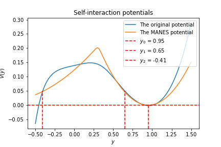
Therefore, instead of literally using Eq.(22) as a specification of the self-interaction potential $V(y)$, this work will assume a confining potential that may be a single-well or a multi-well potential, depending on the model parameters. Confining potentials are easier to work with than non-confining ones, as they give rise to discrete spectra and stationary states in the long run $t\rightarrow\infty$, which would not exist for non-confining potentials. For a multi-well potential with two or more local minima, the model dynamics would be similar to the Desai-Zwanzig model [3] which chooses a symmetric quartic double well potential as a model of $V(y)$, and its generalized version in [8] that considers more complex multi-well potentials. The next section provides details of the MANES potential that will be used later in this paper for the analysis of dynamics and phase structure of the model.

In this paper, the dynamics implied by the Langevin equation (20) are explored using a simple and highly tractable non-linear self-interaction potential $V(y)$ given by the logarithm of a two-component Gaussian Mixture (GM):

$$V(y)=-h^{2}\log\left[(1-a)\phi(y|\mu_{1}T,\sigma_{1}^{2}T)+a\phi(y|\mu_{2}T,\sigma_{2}^{2}T)\right]-h^{2}\log C+V_{0}$$

(23)

where $\phi(y|\mu,\sigma^{2})$ is a Gaussian density, $C$ is a constant that will be defined below, and $V_{0}$ is another constant chosen such that the minimum value of $V(y)$ is zero. This potential was introduced in [10] within the context of a model for a single stock called the Non-Equilibrium Skew (NES) model. The choice (23) is motivated by both the ease of the analytical treatment and the flexibility of the parametric family described by Eq.(23) which, depending on parameters, describes either a single-well anharmonic potential or a double-well potential. As market flows and their price impact produce a nonlinear potential, the parametric family of potentials presented by Eq.(23) make it possible for the model to capture these effects. As the present work can be considered a multi-asset (MA) generalization of the NES model, in what follows I will refer to the form in Eq.(23) as the MANES potential.

As explained in more detail in [10], the MANES potential (23) can also be represented as

$$V(y)=-h^{2}\log\Psi_{0}(y)+V_{0},\;\;\;\Psi_{0}(y):=C\left[(1-a)\phi(y|\mu_{1}T,\sigma_{1}^{2}T)+a\phi(y|\mu_{2}T,\sigma_{2}^{2}T)\right]$$

(24)

where $\Psi_{0}(y)$ is the ground state wave function (WF) of a quantum mechanical system corresponding to the classical stochastic dynamics with potential $V(y)$ [10].¹¹¹¹ 11 A Gaussian mixture can approximate a ground state wave function of a particle placed in either a single well or a double well potential. Double well potentials play a special role in statistical physics and quantum mechanics, and are often used to model tunneling phenomena, see e.g. [12] or [18]. In particular, a symmetric double well is described by a symmetric version of $\Psi_{0}$ with $a=1/2$ and $\mu_{1}=-\mu_{2},\,\sigma_{1}=\sigma_{2}$. For other choices of model parameters, the GM model for function $\Psi_{0}$ can fit a variety of shapes including both a unimodal and bimodal shapes. In what follows, the WF (24) will be occasionally referred to as the MANES WF. The stationary state of the original classical stochastic dynamics is then given by its square $\Psi_{0}^{2}(y)$. The constant $C$ introduced in (23) is in fact a normalization constant that can be obtained from the requirement that the ground state WF $\Psi_{0}$ is squared-normalized, i.e. $\int dy\Psi_{0}^{2}(y)=1$. Note that while $\Psi_{0}(y)$ is proportional to a two-component Gaussian mixture, its square is proportional to a three-component Gaussian mixture:

	$\displaystyle\Psi_{0}^{2}(y)$	$\displaystyle=$	$\displaystyle\frac{C^{2}}{2\sqrt{\pi T}}\left[\frac{(1-a)^{2}}{\sigma_{1}}\phi\left(y|\mu_{1}T,\frac{\sigma_{1}^{2}}{2}T\right)+\frac{a^{2}}{\sigma_{2}}\phi\left(y|\mu_{2}T,\frac{\sigma_{2}^{2}}{2}T\right)\right.$		(25)
		$\displaystyle+$	$\displaystyle\left.\frac{2a(1-a)}{\sqrt{(\sigma_{1}^{2}+\sigma_{2}^{2})/2}}e^{-\frac{(\mu_{1}-\mu_{2})^{2}T}{2(\sigma_{1}^{2}+\sigma_{2}^{2})}}\phi\left(y|\mu_{3}T,\frac{\sigma_{3}^{2}}{2}T\right)\right]$

where the additional third Gaussian component has the following mean and variance:

$$\mu_{3}:=\frac{\mu_{1}\sigma_{2}^{2}+\mu_{2}\sigma_{1}^{2}}{\sigma_{1}^{2}+\sigma_{2}^{2}},\;\;\;\frac{\sigma_{3}^{2}}{2}=\frac{\sigma_{1}^{2}\sigma_{2}^{2}}{\sigma_{1}^{2}+\sigma_{2}^{2}}$$

(26)

The normalization condition thus fixes the value of the constant $C$ as follows:

$$C^{2}=\frac{2\sqrt{\pi T}}{\Omega},\;\;\;\text{where}\;\;\;\Omega=\frac{(1-a)^{2}}{\sigma_{1}}+\frac{a^{2}}{\sigma_{2}}+\frac{2a(1-a)}{\sqrt{(\sigma_{1}^{2}+\sigma_{2}^{2})/2}}e^{-\frac{(\mu_{1}-\mu_{2})^{2}T}{2(\sigma_{1}^{2}+\sigma_{2}^{2})}}$$

(27)

The three-component Gaussian mixture density $\Psi_{0}^{2}(y)$ given by Eq.(25) can be written more compactly using Gaussian mixture weights

$$\omega_{1}:=\frac{(1-a)^{2}}{\sigma_{1}\Omega},\;\;\;\omega_{2}:=\frac{a^{2}}{\sigma_{2}\Omega},\;\;\;\omega_{3}:=\frac{2a(1-a)}{\Omega\sqrt{(\sigma_{1}^{2}+\sigma_{2}^{2})/2}}e^{-\frac{(\mu_{1}-\mu_{2})^{2}T}{2(\sigma_{1}^{2}+\sigma_{2}^{2})}},\;\;\;\sum_{i=1}^{3}\omega_{i}=1$$

(28)

This produces the following three-component Gaussian mixture model for the stationary distribution $p_{s}(y)=\Psi_{0}^{2}(y)$:

$$p_{s}(y)=\sum_{k=1}^{3}\omega_{k}\phi\left(y|\mu_{k}T,\frac{\sigma_{k}^{2}}{2}T\right)$$

(29)

Examples of trial ground state WFs $\Psi_{0}$ and resulting potentials $V(y)$ are shown in Fig. 2.

While this expression produces a non-linear behavior for small positive or negative values of $y$, its limiting behavior at $y\rightarrow\pm\infty$ is rather simple and coincides with a harmonic (quadratic) potential:

$$\left.V(y)\right|_{y\rightarrow-\infty}=h^{2}\frac{(y-\mu_{2}T)^{2}}{2\sigma_{2}^{2}T},\;\;\;\left.V(y)\right|_{y\rightarrow\infty}=h^{2}\frac{(y-\mu_{1}T)^{2}}{2\sigma_{1}^{2}T}\;\;\;\;(\mu_{2}<\mu_{1})$$

(30)

The fact that the limiting behavior of the potential coincides with a harmonic potential as $y\rightarrow\pm\infty$ means that in this asymptotic regime the model behavior is described by a harmonic oscillator, and thus is fully analytically tractable.

For small values $y\ll 1$, the NES potential (23) can provide a good approximation to a quartic potential that we found for small values $y\ll 1$ in the previous analysis, see Eq.(22). On the other hand, the asymptotic behavior of the NES potential (23) which coincides with a harmonic potential as $|y|\rightarrow\infty$ is different from the asymptotically quartic potential implied by Eq.(22). However, if the ‘physics’ of the system is determined by a region of small values of $y$, replacing an asymptotically quartic potential by an asymptotically harmonic potential should produce a negligible impact on observable consequences of the model while significantly simplifying the analysis.

As Gaussian mixtures are known to be universal approximations for an arbitrary non-negative functions given enough components, this implies that an arbitrary potential that asymptotically coincides with a harmonic oscillator potential can be represented as a negative logarithm of a Gaussian mixture. We can refer to such class of potentials as Log-Gaussian Mixture (LGM) potentials. In this paper, I only consider a two-component LGM potential.¹²¹² 12 A requirement of an asymptotic harmonic oscillator behavior could be seen as a potential limitation for the LGM class of potentials, as many interesting potentials have a different asymptotic behavior. To this point, we can note that an onset of such a quadratic regime can always be pushed further away by a proper rescaling of the coordinate, while for small or moderate values of a new rescaled argument, the dynamics can still be arbitrarily non-linear, and driven by the number of Gaussian components and their parameters.

While with general parameters $\mu_{1}\neq\mu_{2},\sigma_{1}\neq\sigma_{2}$ and $a\neq 1/2$ the potential (24) is non-symmetric under reflections $y\rightarrow-y$, it becomes symmetric, with $V(-y)=V(y)$, for the special choice $\mu_{1}=-\mu_{2}=\mu$, $\sigma_{1}=\sigma_{2}=\sigma$ and $a=1/2$, see Fig. 2. It is useful for what follows to consider a potential which is only slightly asymmetric. This can be done by considering the following specification of model parameters in (24):

$$a=\frac{1}{2}+\varepsilon_{a},\;\;\;\mu_{1,2}=\pm\mu+\varepsilon_{\mu},\;\;\;\sigma_{1,2}^{2}=\sigma^{2}\pm\varepsilon_{\sigma}$$

(31)

with small parameters $\varepsilon_{a},\varepsilon_{\mu},\varepsilon_{\sigma}\ll 1$. Using these parameters in Eq.(24), we obtain, to the linear order in the asymmetry,

$$V(y)=V^{(s)}(y)-B_{0}y$$

(32)

where $V^{(s)}(y)=-h^{2}\log\Psi_{0}^{(s)}(y)+V_{0}$ is a symmetric potential with $V^{(s)}(y)=V^{(s)}(-y)$,

$$\Psi_{0}^{(s)}(y):=\frac{C}{2}\left[\phi(y|\mu T,\sigma^{2}T)+\phi(y|-\mu T,\sigma^{2}T)\right]$$

(33)

is a symmetric ground state wave function, and parameter $B_{0}$ is a linear function of $\varepsilon_{a},\,\varepsilon_{\mu},\,\varepsilon_{\sigma}$:

$$B_{0}=\frac{h^{2}}{\sigma^{2}T}\left[\left(1-\frac{\mu^{2}}{\sigma^{2}}\right)\varepsilon_{\mu}+\frac{\mu}{\sigma^{2}}\left(1-\frac{\mu^{2}}{2\sigma^{2}}\right)\varepsilon_{\sigma}\right]-\frac{2\mu h^{2}}{\sigma^{2}}\varepsilon_{a}$$

(34)

Eq.(32) shows that a slightly asymmetric potential corresponding to model parameters in Eq.(31) can be approximated for small values of $y$ by adding a linear term to the potential $V^{(s)}(y)$ obtained in the symmetric limit, where the coefficient $B_{0}$ can be directly computed from the original model parameters. As the term $B_{0}y$ in Eq.(32) can be interpreted as the contribution of an external field $B_{0}$ to the potential energy of the oscillator $y$, this implies that the dynamics in a slightly asymmetric potentials $V(y)$ can be approximated by the dynamics in a symmetric potential $V^{(s)}(y)$ with an additional fictitious external field $B_{0}$. This observation will be used below.

Now, after we specified the particular self-interaction MANES potential $V(y)$ given by Eq.(23), we proceed with an equivalent probabilistic approach to the dynamics described by the Langevin equation (20). Such probabilistic method is provided by a corresponding Fokker-Planck equation (FPE). This approach will be presented in the next two sections. Note that in both of them the explicit form of the potential $V(y)$ is not used, and thus all equations in this section and the next Sect. 3.4 are general and valid for an arbitrary confining potential $V(y)$.

The FPE corresponding to the Langevin equation (20) is a linear partial differential equation for the joint probability $P({\bf y},t)=P(y_{1},\ldots,y_{N},t)$ of a state ${\bf y}=\left[y_{1},\ldots,y_{N}\right]$ describing $N$ stocks at time $t$, given an initial position ${\bf y}_{0}$ at time $t=0$:

$$\frac{\partial P({\bf y},t)}{\partial t}=\sum_{i=1}^{N}\frac{\partial}{\partial y_{i}}\left[\left(\frac{\partial V(y_{i})}{\partial y_{i}}+\frac{g}{N}\sum_{j=1}^{N}\frac{\partial V_{int}(y_{i}-y_{j})}{\partial y_{i}}\right)P({\bf y},t)+\frac{h^{2}}{2}\frac{\partial}{\partial y_{i}}P({\bf y},t)\right]$$

(35)

For applications, the most interesting probability distributions for a system of identical non-linear oscillators are one-particle density $P^{(1)}$ and pair-density function $P^{(2)}$ defined as follows:

$$P^{(1)}(y,t)=\int dy_{2},\ldots,dy_{N}P(y,y_{2},\ldots,y_{N},t),\;\;\;P^{(2)}(y,y^{\prime},t)=\int dy_{3},\ldots,dy_{N}P(y,y^{\prime},y_{3},\ldots,y_{N},t)$$

(36)

Integrating over $y_{2},\ldots,y_{N}$ in the FPE (35), we obtain

$$\frac{\partial P^{(1)}(y,t)}{\partial t}=\frac{\partial}{\partial y}\left[\frac{\partial V(y)}{\partial y}P^{(1)}(y,t)+\frac{h^{2}}{2}\frac{\partial}{\partial y}P^{(1)}(y,t)+g\int dy^{\prime}\frac{\partial V_{int}(y-y^{\prime})}{\partial y}P^{(2)}(y,y^{\prime},t)\right]$$

(37)

Note that while a single-particle FPE is a partial differential equation (PDE) for a one-particle density, Eq.(37) is an integro-differential equation that relates two different densities $P^{(1)}$ and $P^{(2)}$. Due to multi-body interactions whose strength is controlled by the coupling constant $g$, the densities $P^{(1)}$ and $P^{(2)}$ are coupled in Eq.(37) which in fact represents the first equation in an infinite hierarchy of the BBGKY type, see e.g. [16].

To proceed, I follow the traditional approach in the physics literature (see e.g. [14], [8]), and rely on the mean field approximation (MFA) where the probability density factorizes into a product of single-particle densities:

$$P(y_{1},\ldots,y_{N},t)=\prod_{i=1}^{N}p(y_{i},t)$$

(38)

Therefore, with the MFA, dynamics amounts to a system of $N$ independent and identical particles, such that the coordinate of any of them is given by the average $\frac{1}{N}\sum_{i=1}^{N}y_{i}$ of all original (interacting) particles in the system. This approximation becomes exact in the thermodynamic limit $N\rightarrow\infty$.

Note that the mean field $\frac{1}{N}\sum_{i=1}^{N}y_{i}$ of a homogeneous system of identical non-linear oscillators can be viewed as a reasonable proxy to the market returns, which are usually proxied by returns of the S&P 500 index. Of course, the real stock market is quite heterogeneous, and furthermore different firms are weighted in the S&P 500 index by their total capitalization. Therefore, identifying the mean field $\frac{1}{N}\sum_{i=1}^{N}y_{i}$ for a homogeneous system with market returns is not expected to provide a good approximation for the price dynamics of any individual stock. However, more importantly, the present mean field approach emphasizes the difference between a single-stock dynamics and the group dynamics of a market made of many stocks, while still retaining a link between them and keeping the whole approach practical.

Plugging the MFA ansatz (38) into Eq.(37), we obtain

$$\frac{\partial p(y,t)}{\partial t}=\frac{\partial}{\partial y}\left[\frac{\partial V(y)}{\partial y}p(y,t)+\frac{h^{2}}{2}\frac{\partial}{\partial y}p(y,t)+gp(y,t)\frac{\partial}{\partial y}\int dy^{\prime}V_{int}(y-y^{\prime})p(y^{\prime},t)\right]$$

(39)

This non-linear integro-differential equation holds for an arbitrary interaction potential $V_{int}(y-y^{\prime})$. For a particular case of the quadratic Curie-Weiss potential (21), Eq.(39) produces the following equation:

$$\frac{\partial p(y,t)}{\partial t}=\frac{\partial}{\partial y}\left[\frac{\partial V(y)}{\partial y}p(y,t)+\frac{h^{2}}{2}\frac{\partial}{\partial y}p(y,t)+g\left(y-\langle y\rangle_{p}\right)p(y,t)\right],\;\;\;\;\langle y\rangle_{p}:=\int dyyp(y,t)$$

(40)

This equation is non-linear due to the dependence of the coefficient $\left(y-\langle y\rangle_{p}\right)$ in the last term on the density $p(y,t)$. The nonlinear Fokker-Planck equation (40) is known in the literature as the McKean-Vlasov equation [15, 2, 4]. Critically important is the fact the unlike the initial linear FPE equation (35) for a finite $N$-particle system, the the McKean-Vlasov equation that describes the thermodynamic limit $N\rightarrow\infty$ is nonlinear. As a result, it produces far richer dynamics including phase transitions [2].

Note that if we formally treat $\langle y\rangle_{p}$ as an independent parameter, the McKean-Vlasov equation (40) can be viewed as a linear FPE with the following ’effective’ potential:

$$V_{eff}(y)=V(y)+g\left(\frac{y^{2}}{2}-my\right),\;\;\;m:=\langle y\rangle_{p}$$

(41)

The stationary density for a given value of $m=\langle y\rangle_{p}$ is therefore obtained as a Boltzmann distribution with the ‘inverse temperature’ $\beta=2/h^{2}$:

$$p(y|m)=\frac{1}{Z(m)}e^{-\frac{2}{h^{2}}\left[V(y)+g\left(\frac{y^{2}}{2}-my\right)\right]},\;\;\;Z(m):=\int dye^{-\frac{2}{h^{2}}\left[V(y)+g\left(\frac{y^{2}}{2}-my\right)\right]}$$

(42)

This solution should satisfy the self-consistency condition for $m=\langle y\rangle_{p}=\int dyyp(y,t)$:

$$m=\frac{1}{Z(m)}\int dyye^{-\frac{2}{h^{2}}\left[V(y)+g\left(\frac{y^{2}}{2}-my\right)\right]}$$

(43)

Once the value of $m$ is found by solving the self-consistency equation (43), it is substituted back to Eq.(42) to find the stationary density. The number of equilibrium states in the system is therefore given by the number of solutions to Eq.(43). The solution of this equation for the MANES potential will be presented below in Sect. 4.

As was noted above, the McKean-Vlasov equation (40) can be viewed as a single-particle linear FPE with the effective potential (41) that I repeat here for convenience:

$$V_{eff}(y)=V(y)+g\left(\frac{y^{2}}{2}-my\right),\;\;\;m:=\langle y\rangle_{p}$$

(44)

provided $m$ is found from self-consistency equations that would be introduced below. However, prior to this, we can note that for the specific choice of the NES potential (23), the effective potential $V_{eff}(y)$ will have exactly the same functional form as the single-stock potential $V(y)$, albeit with different parameters. Using the physics nomenclature, one can say that parameters of the original single-particle system are renormalized by interactions which are represented by the second term in Eq.(44).

To find the new renormalized parameters, we write Eq.(44) using Eq.(23) as follows:

	$\displaystyle V_{eff}(y)=-h^{2}\log\left[(1-a)\phi(y|\mu_{1}T,\sigma_{1}^{2}T)+a\phi(y|\mu_{2}T,\sigma_{2}^{2}T)\right]-h^{2}\log e^{-g\frac{(y-m)^{2}}{2h^{2}}+g\frac{m^{2}}{2h^{2}}}$
	$\displaystyle=-h^{2}\log\left[e^{-g\frac{(y-m)^{2}}{2h^{2}}+g\frac{m^{2}}{2h^{2}}}\left((1-a)\phi(y|\mu_{1}T,\sigma_{1}^{2}T)+a\phi(y|\mu_{2}T,\sigma_{2}^{2}T)\right)\right]$		(45)
	$\displaystyle=-h^{2}\log\left[(1-\bar{a})\phi(y|\bar{\mu}_{1}T,\bar{\sigma}_{1}^{2}T)+\bar{a}\phi(y|\bar{\mu}_{2}T,\bar{\sigma}_{2}^{2}T)\right]-h^{2}\hat{V}(m)$

where $\bar{\mu}_{1},\bar{\mu}_{2},\bar{\sigma}_{1},\bar{\sigma}_{2},\bar{a}$ are new ‘renormalized’ parameters for a single-particle NES potential, and $\hat{V}(m)$ stands for terms that depend on $m$ but not on $y$. They can be easily computed using the well-known relation expressing a product of two Gaussian densities as a rescaled third Gaussian density:

$$\phi(y|\mu_{1},\sigma_{1}^{2})\phi(y|\mu_{2},\sigma_{2}^{2})=\frac{S_{12}}{\sqrt{2\pi\sigma_{12}^{2}}}\exp\left[-\frac{(y-\mu_{12})^{2}}{2\sigma_{12}^{2}}\right]=S_{12}\phi(y|\mu_{12},\sigma_{12}^{2})$$

(46)

where

$$\sigma_{12}^{2}=\frac{\sigma_{1}^{2}\sigma_{2}^{2}}{\sigma_{1}^{2}+\sigma_{2}^{2}},\;\;\;\mu_{12}=\left(\frac{\mu_{1}}{\sigma_{1}^{2}}+\frac{\mu_{2}}{\sigma_{2}^{2}}\right)\sigma_{12}^{2},\;\;\;S_{12}=\frac{1}{\sqrt{2\pi\left(\sigma_{1}^{2}+\sigma_{2}^{2}\right)}}\exp\left[-\frac{(\mu_{1}-\mu_{2})^{2}}{2\left(\sigma_{1}^{2}+\sigma_{2}^{2}\right)}\right]$$

(47)

Using these relations, we obtain the renormalized parameters and the function $\hat{V}(m)$:

	$\displaystyle\bar{\mu}_{k}=\frac{\mu_{k}+\frac{g}{h^{2}}\sigma_{k}^{2}m}{1+\frac{g}{h^{2}}\sigma_{k}^{2}T},\;\;\bar{\sigma}_{k}^{2}=\frac{\sigma_{k}^{2}}{1+\frac{g}{h^{2}}\sigma_{k}^{2}T},\;\;k=1,2$
	$\displaystyle\bar{a}=\left[1+\frac{1-a}{a}\sqrt{\frac{h^{2}+g\sigma_{2}^{2}T}{h^{2}+g\sigma_{1}^{2}T}}e^{\frac{g(m-\mu_{2}T)^{2}}{2(h^{2}+g\sigma_{2}^{2}T)}-\frac{g(m-\mu_{1}T)^{2}}{2(h^{2}+g\sigma_{1}^{2}T)}}\right]^{-1}$		(48)
	$\displaystyle\hat{V}(m)=\frac{gm^{2}}{2h^{2}}+\log\left(\frac{(1-a)h}{\sqrt{h^{2}+g\sigma_{1}^{2}T}}e^{-\frac{g(m-\mu_{1}T)^{2}}{2(h^{2}+g\sigma_{1}^{2}T)}}+\frac{ah}{\sqrt{h^{2}+g\sigma_{2}^{2}T}}e^{-\frac{g(m-\mu_{2}T)^{2}}{2(h^{2}+g\sigma_{2}^{2}T)}}\right)$

These formulae show that additional quadratic and linear terms in Eq.(44) can be re-absorbed into rescaled parameters of the Gaussian mixture, where the Gaussian means become linear functions of the mean field $m$, while the mixing coefficient depends on $m$ non-linearly. This implies that within the mean field approximation, the dynamics of market log-returns can be modeled as the dynamics of a fictitious single stock, with initial single-stock model’s parameters being ’dressed’ by interactions according to Eq.(3.5).

References

- [1] J.P. Bouchaud, “The Inelastic Market Hypothesis: A Microstructural Interpretation”, https://papers.ssrn.com/sol3/papers.cfm?abstract_id=3896981 (2021)
- [2] D.A. Dawson, “Critical Dynamics and Fluctuations for a Mean-Field Model of Cooperative Behavior”, J. Stat. Phys., 31(1), 29-85 (1983).
- [3] R.C. Desai amd R. Zwanzig, “Statistical Mehanics of a Nonlinear Stochastic Model”, Journal of Stat. Physics, 19(1) 1-24 (1978).
- [4] T.D. Frank, Nonlinear Fokker-Planck Equations, Springer Series in Synergetics, Springer-Verlag, Berlin (2005).
- [5] A. Frazzini and O.A. Lamont, ”Dumb Money: Mutual Fund Flows and the Cross-Section of Stock Returns”, Journal of Financial Economics, Elsevier, vol. 88(2), pages 299-322 (2008).
- [6] X. Gabaix and R.S.J. Koijen, “In Search of the Origins of Financial Fluctuations: The Inelastic Markets Hypothesis”, Swiss Finance Institute Research Paper Series (2020), https://papers.ssrn.com/sol3/papers.cfm?abstract_id=3686935#
- [7] G. Gemmill and A. Saflekos, “How Useful are Implied Distributions? Evidence from Stock-Index Options” (2000), The Journal of Derivatives, 7 (3), 83-91 (2000), available at https://www.bis.org/publ/bisp06e.pdf.
- [8] S.N. Gomes, S. Kalliadis, G.A. Pavlotis, P. Yatsyshin, “Dynamics of the Desai-Zwanzig Model in Multi-Well and Random Energy Landscapes”, https://arxiv.org/abs/1810.06371 (2019).
- [9] I. Halperin and M.F. Dixon, “Quantum Equilibrium-Disequilibrium: Asset Price Dynamics, Symmetry Breaking, and Defaults as Dissipative Instantons”, Physica A 537, 122187, https://doi.org/10.1016/j.physa.2019.122187 (2020).
- [10] I. Halperin, “Non-Equilibrium Skewness, Market Crises, and Option Pricing: Non-Linear Langevin Model of Markets with Supersymmetry”, Physica A 594, 127065, https://doi.org/10.1016/j.physa.2022.127065 (2022).
- [11] I. Halperin, “The Inverted World of Classical Quantitative Finance: a Non-Equilibrium and Non-Perturbative Finance Perspective”, https://arxiv.org/abs/2008.03623 (2020).
- [12] L.D. Landau and E.M. Lifschitz, Quantum Mechanics, Elsevier (1980).
- [13] P. Langevin, “Sur la Théorie du Mouvement Brownien”, Comps Rendus Acad. Sci. (Paris) 146, 530-533 (1908).
- [14] N. Martzel and C. Aslangul, “Mean-Field Treatment of the Many-Body Fokker-Planck Equation”, https://arxiv.org/abs/cond-mat/0106101 (2001).
- [15] H.P. McKean, Jr., “A Class of Markov Processes Associated with Nonlinear Parabolic Equations”, Proc. Nat. Acad. Sci. USA, 56 pp. 1907-1911, (1966).
- [16] D.A. McQuarrie, Statistical Mechanics, Harper & Row, New York (1973).
- [17] P.S. Stilger, A. Kostakis, and S.H. Poon, “What Does Risk-Neutral Skewness Tell Us About Future Stock Returns?”, Management Science, vol. 63, Issue 3, 1657-2048 (2016).
- [18] C. Zinn-Justin, Quantum Field Theory and Critical Phenomena, Fourth Edition, Clarendon Press, Oxford (2002).