Parametric invariance

In a paper of 1902 rayleigh1902, Rayleigh analyzed a simple pendulum with its string being varied very slowly. Motivated by the theoretical demonstration of the radiation pressure by Maxwell and its experimental confirmation by Lebedev, Rayleigh inquired whether any other kinds of vibration, such as sound vibrations, would also cause pressure. To answer this question, he posed the problem of finding the force acted by a vibrating pendulum on its pivot when its length changes slowly and continuously with time.

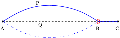
The length of the pendulum is changed by the use of a ring through which passes the string, as shown in figure 1. The ring is constrained to move vertically and as it moves the length BC of the pendulum changes although the total length ABC remains constant. The problem is to determine the force that tends to move the ring upwards as the pendulum swings.

The ring is acted by two vertical forces, one of them is upward and equal to the tension $\Gamma$ of the string and the other is downward and equal to $\Gamma\cos\theta$ where $\theta$ is the angle BCD. The net upward force on the ring is thus $F=\Gamma(1-\cos\theta)$. Now the potential energy of the pendulum is $V=P\ell(1-\cos\theta)$ where $P$ is the weight of the bob, and $\ell$ is the length BC of the pendulum. Considering that for small oscillations $\Gamma$ is approximately equal to $P$, one finds $F=V/\ell$. As the mean value of the potential energy is one half of the total energy $E$ of the pendulum, Rayleigh concludes that the upward mean force $F$ on the ring is

$$F=\frac{E}{2\ell}.$$

(24)

As the work done on the ring is equal to decrease in the energy of the pendulum, then $dE=-Fd\ell$, and $dE=-Ed\ell/2\ell$ which by integration gives $E=a/\sqrt{\ell}$, where $a$ is a constant. Although, Rayleigh did not mention it explicitly, it follows from this result that the quantity

$$I=E\sqrt{\ell}$$

(25)

is an invariant quantity when the length of the pendulum changes slowly with time. As the frequency of oscillation $\omega$ of a simple pendulum executing small oscillations is inversely proportional to $\sqrt{\ell}$ it follows that the quantity

$$I=\frac{E}{\omega}$$

(26)

is an invariant as well.

Rayleigh also treated in the same paper the problem of the force exerted by a vibrating stretched string on the points where it is attached. One end of the stretched string is fixed and the other is allowed to move by the use of a ring as shown in figure 2. The position of the ring determines the length of the vibrating string, which we denote by $\ell$. Rayleigh argues that the mean force $F$ acting on the ring is related to the total energy $E$ of the vibrating string by

$$F=\frac{E}{\ell},$$

(27)

and is thus equal to the energy per unit length. Again, the work done on the ring equals the decrease in energy, $dE=-Fd\ell=-Ed\ell/\ell$ and, after integration, $E=a/\ell$ where $a$ is a constant, and now $E$ is inversely proportional to $\ell$. Thus,

$$I=E\ell$$

(28)

is invariant.

The main result of the approach by Rayleigh can be stated as follows. Let us consider a periodic system and the force $f$ acted by the system on the environment at a point which moves as a result of the change of a parameter $\lambda$. As the system is periodic the force $f$ oscillates in time but its time average $F$ over one cycle is nonzero. If the parameter changes slowly $F$ varies slowly and so does the energy $E$ of the system. These two quantities are related by

$$\frac{dE}{d\lambda}=-F,$$

(29)

if the parameter changes very slowly with time. To show this result we proceed as follows.

We consider a system with several degrees of freedom described by the Lagrangian $L=K-V$, where $K$ is the kinetic energy and $V$ is the potential energy. The Lagrangian $L(q,\dot{q},\lambda)$ depends on the coordinates $q_{i}$ and velocities $\dot{q}_{i}$, which we are denoting collectively by $q$ and $\dot{q}$, respectively, and on a parameter $\lambda$ which depends on time. The Lagrange equations of motion are

$$\frac{d}{dt}\frac{\partial L}{\partial\dot{q}_{i}}=\frac{\partial L}{\partial q_{i}}.$$

(30)

If we define the momentum

$$p_{i}=\frac{\partial L}{\partial\dot{q}},$$

(31)

then the equations of motion are written as

$$\frac{dp_{i}}{dt}=\frac{\partial L}{\partial q_{i}},$$

(32)

and the differential of $L$ as

$$dL=\sum_{i}p_{i}d\dot{q}_{i}+\sum_{i}\dot{p}_{i}dq+\frac{\partial L}{\partial t}dt.$$

(33)

If we perform the Legendre transformation

$$H=\sum_{i}p_{i}\dot{q}_{i}-L,$$

(34)

then

$$dH=\sum_{i}\dot{q}_{i}dp_{i}-\sum_{i}\dot{p}_{i}dq-\frac{\partial L}{\partial t}dt,$$

(35)

from which follows the Hamilton equations of motion

$$\dot{q}_{i}=\frac{\partial H}{\partial p_{i}},\qquad\qquad\dot{p}_{i}=-\frac{\partial H}{\partial q_{i}},$$

(36)

where $H(q,p,\lambda)$ is the Hamiltonian, a function of the coordinates and momenta, and depends on time through the parameter $\lambda$. It also follows that

$$\frac{\partial H}{\partial t}=-\frac{\partial L}{\partial t},$$

(37)

where the first derivative is determined at constant $q$ and $p$ whereas the second at constant $q$ and $\dot{q}$.

The Hamiltonian $H$ equals the total energy $K+V$ if $K$ is a quadratic form in the velocities. Its variation with time is

$$\frac{dH}{dt}=\frac{\partial H}{\partial t},$$

(38)

and as it depends on time through the parameter $\lambda$, it is not conserved. Defining the function $f$ by

$$f=-\frac{\partial H}{\partial\lambda},$$

(39)

the equation (38) can be written as

$$\frac{dH}{dt}=-cf,$$

(40)

where $c=d\lambda/dt$ is the rate of variation of the parameter.

Now we proceed as follows. We divide the time axis into intervals equal to the cycle period $T$. The integration of the equation (40) over one cycle beginning at time $t_{0}$ and ending at time $t_{1}$ gives

$$\frac{\Delta H}{T}=-\frac{1}{T}\int_{t_{0}}^{t_{1}}cf(q,p,\lambda)\,dt,$$

(41)

where

$$\Delta H=H(q_{1},p_{1},\lambda_{1})-H(q_{0},q_{0},\lambda_{0}),$$

(42)

and the subindexes refer to the beginning and ending of the interval.

We use an approximation in which the trajectory in phase space is replaced by a trajectory $(x(t),y(t))$ which is the solution of the equations of motion by considering that the parameter $\lambda$ is kept unchanged and equal to its value at the beginning at the interval. The variation of $H$ becomes

$$\Delta H=H(x_{1},y_{1},\lambda_{1})-H(x_{0},y_{0},\lambda_{0}).$$

(43)

The variation $\Delta\lambda=\lambda_{1}-\lambda_{0}$ of the parameter in the interval is equal to $\Delta\lambda=Tc$ and $c$ is small because the parameter varies slowly with time. Therefore $\Delta H/T=c\Delta H/\Delta\lambda$ can be approximated by

$$c\frac{d}{d\lambda}H(x,y,\lambda),$$

(44)

calculated at the beginning at the interval.

Using again the same approximation, we replace $q$ by $x(t)$, and $p$ by $y(t)$ in the right hand side of (41). Defining

$$F=\frac{1}{T}\int_{t_{0}}^{t_{1}}f(x,y,\lambda)dt,$$

(45)

the equation (41) becomes

$$\frac{dE}{d\lambda}=-F,$$

(46)

where $c$ was assumed $c$ to be constant during the cycle. In this equation, $E$ is equal to $H(x,y,\lambda)$ and depends only on $\lambda$ because it is conserved along one cycle, and the quantity $F$ is understood as the time average of $f$ along one cycle and also depends only on $\lambda$. Since $F$ is a function of $\lambda$, this relation is understood as a differential equation in $\lambda$. Its solution gives the explicit dependence of $E$ on $\lambda$, and on time since $\lambda$ is a given function of time.

Let us use the notation

$$\overline{f}=\frac{1}{T}\int_{t_{0}}^{t_{0}+T}fdt,$$

(47)

for the time average of $f$ over one cycle of period $T$. The function $f$ depends on the parameter $\lambda$, which is considered to be fixed. The main result can then be written in the abbreviated form

$$\frac{dE}{d\lambda}=\overline{\frac{\partial{\cal H}}{\partial\lambda}},$$

(48)

and $E=\overline{\cal H}$. Notice that, as ${\cal H}$ is conserved if $\lambda$ is fixed, then $E$ coincides with $E={\cal H}$ during one period and this time average is immaterial.

Let us apply this approach to the Rayleigh pendulum The Lagrangian function is given by

$$L=\frac{1}{2}m\ell^{2}\dot{\theta}^{2}-\frac{1}{2}mg\ell\theta^{2}.$$

(49)

To determined $f=-\partial H/\lambda$, we observe that using the equality (37), it can also be determined by $f=\partial L/\partial\lambda$. Deriving $L$ with respect to $\ell$, we find

$$f=m\ell\dot{\theta}^{2}-\frac{1}{2}mg\theta^{2}.$$

(50)

The energy $E$ is given by

$$E=\frac{1}{2}m\ell^{2}\dot{\theta}^{2}+\frac{1}{2}mg\ell\theta^{2}.$$

(51)

The equation of motion, keeping the parameter $\ell$ unchanged is

$$\ell\ddot{\theta}=-g\theta,$$

(52)

whose solution is $\theta=c\cos\omega t$, where $\omega=\sqrt{g/\ell}$. Replacing the solution in the expression for $H$ and $f$, and taking the time average over one cycle, we obtain

$$E=\frac{1}{2}mgc^{2}\ell,\qquad\qquad F=\frac{1}{4}mgc^{2},$$

(53)

which gives $F=E/2\ell$, the result (24). The integration of $dE/d\ell=-F$ gives the result $E\sqrt{\ell}$ an invariant, or $E/\omega$ an invariant, results already found.

For a particle of mass $m$ bounded to a spring of coefficient $k$, the Lagrangian function is

$$L=\frac{1}{2}m\dot{x}^{2}-\frac{1}{2}kx^{2},$$

(54)

and the energy is

$$E=\frac{1}{2}m\dot{x}^{2}+\frac{1}{2}kx^{2}.$$

(55)

The equation of motion is $m\ddot{x}=-kx$ whose solution is $x=a\cos\omega t$, where $\omega=\sqrt{k/m}$. Replacing these results in the expression for the energy, $E=ka^{2}/2$.

Let us suppose that the spring coefficient is the varying parameter. Then $f=-x^{2}/2$ and $F=-a^{2}/4$. Therefore, $F=-E/2k$ and the integration of $dE/dk=-F$ gives $E/\sqrt{k}$ as an invariant, or $E/\omega$.

Suppose now that the mas is the varying parameter. Then, $f=\dot{x}^{2}/2$ and $F=ka^{2}/4m$. Therefore $F=E/2m$ and the integration of $dE/dm=-F$ gives $E\sqrt{m}$ as an invariant, or $E/\omega$.

Another example consists of a free particle of mass $m$ that moves with speed $v$ between two walls that are a distance $\ell$ apart. The mean force $F$ on the wall is the change of its momentum $2mv$ divided by the time $2\ell/v$ between two collisions, that is, $F=mv^{2}/\ell$ Considering that the kinetic energy is $E=mv^{2}/2$ one finds $F=2E/\ell$ and the integration of $dE/dm=-F$ gives $E\ell^{2}$ as an invariant.

Let us consider now the vibrating stretched string. Denoting by $u$ the transverse displacement PQ of the string at the point $Q$ and by $x$ the distance from this point to the fixed end A, as shown in figure 2, the equation of motion for $u$ is the wave equation

$$\frac{\partial^{2}u}{\partial t^{2}}=c^{2}\frac{\partial^{2}u}{\partial x^{2}},$$

(56)

where $c$ is the velocity of the wave and equal to $\sqrt{\Gamma/\mu}$, where $\Gamma$ is the tension of the string and $\mu$ is the mass per unit length. The wave equation is understood as the equation of motion associated to the Lagrangian $L=T-V$ where $K$ is the kinetic energy,

$$K=\frac{\mu}{2}\int_{0}^{\ell}\left(\frac{\partial u}{\partial t}\right)^{2}dx,$$

(57)

and $V$ is the potential energy,

$$V=\frac{\Gamma}{2}\int_{0}^{\ell}\left(\frac{\partial u}{\partial x}\right)^{2}dx.$$

(58)

The energy is $H=T+V$.

With the purpose of revealing the explicit dependence on $\ell$, we change the variable of integration from $x$ to $y=x/\ell$, with the result

$$K=\frac{\mu\ell}{2}\int_{0}^{1}\left(\frac{\partial u}{\partial t}\right)^{2}dy,$$

(59)

and $V$ is the potential energy,

$$V=\frac{\Gamma}{2\ell}\int_{0}^{1}\left(\frac{\partial u}{\partial y}\right)^{2}dy.$$

(60)

Using these expression on $L=K-V$, we determine $f=\partial L/\partial\ell$, which gives the following result $f=H/\ell$, where $H=K+V$. Therefore $F=E/\ell$, which is the result (27), and, using the relation $dE/d\ell=-F$, we find that $E=A/\ell$ and $E\ell$ is an invariant as already found.

The solution of the wave equation for vibrations between the fixed ends at $x=0$ and $x=\ell$ is the standing wave

$$u=A\sin kx\cos\omega t,$$

(61)

where $k=n\pi/\ell$ and $n$ is an integer, and $\omega=kc$. Replacing these results into the expression for $K$ and $V$ and taking the time average over one cycle, we find

$$E=\mu A^{2}c^{2}\frac{n^{2}\pi^{2}}{4\ell}\qquad\qquad F=\mu A^{2}c^{2}\frac{n^{2}\pi^{2}}{4\ell^{2}},$$

(62)

showing that indeed $E=a/\ell$ and $F=E/\ell$.

To demonstrate the invariance of expression (1) or its equivalent form (4) we proceed as follows. We start by writing $F$, given by (45), in the form

$$F=-\frac{1}{T}\int_{0}^{T}\frac{\partial H}{\partial\lambda}dt,$$

(63)

where we have used the expression (39) for $f$, and we are considering the variables $\lambda$ and $t$ independent of each other. Recalling that $E=H$, we obtain

$$\frac{dE}{d\lambda}=\frac{1}{T}\!\sum_{i}\int_{0}^{T}\!\!\left(\frac{\partial H}{\partial p_{i}}\frac{\partial p_{i}}{\partial\lambda}+\sum_{i}\frac{\partial H}{\partial q_{i}}\frac{\partial q_{i}}{\partial\lambda}+\frac{\partial H}{\partial\lambda}\!\right)\!dt.$$

(64)

Replacing it in the equation (46), written in the form

$$\frac{dE}{d\lambda}+F=0,$$

(65)

we find

$$\sum_{i}\int_{0}^{T}\left(\frac{\partial H}{\partial p_{i}}\frac{\partial p_{i}}{\partial\lambda}+\frac{\partial H}{\partial q_{i}}\frac{\partial q_{i}}{\partial\lambda}\right)dt=0.$$

(66)

Using the equations of motion (36), we find

$$\sum_{i}\oint\left(\frac{\partial p_{i}}{\partial\lambda}dq_{i}-\frac{\partial q_{i}}{\partial\lambda}dp_{i}\right)=0,$$

(67)

which can be written in the form

$$\frac{dI}{d\lambda}=0,$$

(68)

where

$$I=\frac{1}{2}\sum_{i}\oint(p_{i}dq_{i}-q_{i}dp_{i}).$$

(69)

An integration by parts gives

$$I=\sum_{i}\oint p_{i}dq_{i}.$$

(70)

Since $dI/d\lambda=0$, it follows that $I$ is indeed an invariant. We recall that this expression can also be written as

$$I=\int_{0}^{T}2Kdt,$$

(71)

where $K$ is the kinetic energy and $T$ is the period of the cycle.

The demonstration just carried out shows that the invariant (70) is a sum terms of the type

$$I_{i}=\oint p_{i}dq_{i}.$$

(72)

It does not say whether or not each term $I_{i}$ is an invariant. However, if the momentum $p_{i}$ in this integral (72) depends only on $q_{i}$, which is a statement that the pair of variables $(q_{i},p_{i})$ is separable from the others, then $I_{i}$ is an invariant, which is the result obtained by Burgers. To show this result, it suffices to write (72) as

$$I_{i}=\int p_{i}\dot{q}_{i}dt.$$

(73)

In this form we see that the integrand is twice the kinetic energy of a system with one degree of freedom, as no other variables are involved. But this is the total kinetic energy of a system with one degree of freedom and is thus the Ehrenfest invariant. It is worth mentioning however that the separation of variables may only occur if an appropriate transformation of variables is performed.

The Ehrenfest invariant for a system with one degree of freedom reduces to the phase integral

$$I=\oint pdq,$$

(74)

where $p$ is the momentum conjugate to $q$. The general form of a Lagrangian describing a conservative system with one degree of freedom is

$$L=\frac{1}{2}m\dot{q}^{2}-V,$$

(75)

where $m$ might depend on $q$, and $V$ is a function of $q$ only, and $p=\partial L/\partial\dot{q}$. As the energy is conserved we write $E=H(q,p)$ which describes a closed curve on the phase space. Solving this equation for $p$ and replacing the result in the phase integral, we find

$$I=2\int\sqrt{2m(E-V)}dq,$$

(76)

where the integral is performed in the interval between the two points of return.

For a particle of mass $m$ under the action of a harmonic force, the energy is given by

$$\frac{p^{2}}{2m}+\frac{1}{2}m\omega^{2}x^{2}=E,$$

(77)

where $\omega$ is the frequency of oscillation. This equation describes in the phase space an ellipse of semi-axis equal to $\sqrt{2mE}$ and $\sqrt{2E/m\omega^{2}}$. The phase integral is the area of this ellipse and equals $2\pi E/\omega$, which is thus an invariant.

Another example is given by a free particle that moves along an axis and collides with walls that are a distance $\ell$ apart. The integral (74) becomes equal to $2p\ell$ which is thus an invariant. Taking into account that the kinetic energy of the particle is $E=p^{2}/2m$, it follows that $E\ell^{2}$ is an invariant as the wall moves slowly.

Let us consider now a particle of mass $m$ moving in a plane under a central force. Using polar coordinates, the Lagrangian is given by

$$L=\frac{1}{2}m(\dot{r}^{2}+r^{2}\dot{\theta}^{2})-V,$$

(78)

where $V$ is the potential that depends on $r$ but not on $\theta$. The momenta conjugate to the $r$ and $\theta$ are, respectively, $p_{r}=m\dot{r}$ and $p_{\theta}=mr^{2}dot\theta$.

One equation of motion is

$$\frac{dp_{r}}{dt}=mr\dot{\theta}^{2}+f,$$

(79)

where $f=-dV/dr$ is the centripetal force. The other equation of motion is $dp_{\theta}/dt=0$ from which follows that the angular momentum $p_{\theta}=mr^{2}\theta$ is constant. Denoting by $a$ this constant, then $\dot{\theta}=a/mr^{2}$ which replaced in the equation of motion for $r$, gives

$$\frac{dp_{r}}{dt}=\frac{a^{2}}{mr^{3}}+f.$$

(80)

This equation tell us that the pair of variables $(r,p_{r})$ is separable and that

$$I_{1}=\oint p_{r}dr$$

(81)

is an invariant.

To determine $I_{1}$ explicitly, we multiply (80) by $p_{r}/m=\dot{r}$ and integrate in time to find

$$\frac{p_{r}^{2}}{2m}+V+\frac{a^{2}}{2mr^{2}}=E,$$

(82)

where $E$ is a constant. Solving for $p_{r}$ and replacing in the integral $I_{1}$, we get

$$I_{1}=2\int\sqrt{2m(E-V)-(a^{2}/r^{2})}\,\,dr.$$

(83)

We remark that the integral

$$I_{2}=\oint p_{\theta}d\theta$$

(84)

is also an invariant, in fact it is a constant, $I_{2}=2\pi a$.

We wish to determine now the invariants of a system with three degrees of freedom corresponding to a particle under the action of a central force as is the case of the Kepler problem where this force is proportional to inverse of the square of the distance born1927b; landau1960; terhaar1964; borghi2013. In spherical coordinates, the variables are separable and for each pair of conjugate variables there corresponds an invariant of the form (74). Using spherical coordinates $r$, $\theta$, and $\phi$, with origin at the center of force, the kinetic energy is given by

$$K=\frac{m}{2}\dot{r}^{2}+\frac{m}{2}r^{2}\dot{\theta}^{2}+\frac{m}{2}r^{2}\dot{\phi}^{2}\sin^{2}\theta,$$

(85)

and the Lagrangian is $L=T-V$ where $V(r)$ is the potential energy that depends on $r$ only.

The conjugate momenta are

$$p_{0}=m\dot{r},$$

(86)

$$p_{1}=mr^{2}\dot{\theta},$$

(87)

$$p_{2}=mr^{2}\sin^{2}\theta\dot{\phi},$$

(88)

and the equations of motion are

$$\frac{dp_{0}}{dt}=mr\dot{\theta}^{2}+mr\sin^{2}\theta\dot{\phi}^{2}+f,$$

(89)

$$\frac{dp_{1}}{dt}=mr^{2}\dot{\phi}^{2}\sin\theta\cos\theta,$$

(90)

$$\frac{dp_{2}}{dt}=0,$$

(91)

where $f=-dV/dr$ is the central force that depends on $r$ only. From the last equation it follows that $p_{2}$ is constant. Setting this constant equal to $a$, then $\dot{\phi}=a/mr^{2}\sin^{2}\theta$, which replaced in the equation of motion for $p_{1}$ gives

$$\frac{dp_{1}}{dt}=\frac{a^{2}\cos\theta}{mr^{2}\sin^{3}\theta}.$$

(92)

Multiplying this equation by $p_{1}=mr^{2}\dot{\theta}$ and integrating in time, we find

$$p_{1}^{2}+\frac{a^{2}}{\sin^{2}\theta}=b^{2},$$

(93)

where $b$ is a constant. Therefore $p_{1}$ in the integral

$$I_{1}=\oint p_{1}d\theta$$

(94)

depends only on $\theta$ and is an invariant.

Let us write equation (89) in the form

$$\frac{dp_{0}}{dt}=\frac{p_{1}^{2}}{mr^{3}}+\frac{p_{2}^{2}}{mr^{3}\sin^{2}\theta}+f.$$

(95)

Replacing the result (93) in this equation and bearing in mind that $p_{2}=a$, we find

$$\frac{dp_{0}}{dt}=\frac{b^{2}}{mr^{3}}+f.$$

(96)

Multiplying by $p_{0}/m=\dot{r}$ and integrating in time, we find

$$\frac{p_{0}^{2}}{2m}+V+\frac{b^{2}}{2mr^{2}}=E,$$

(97)

where $E$ is a constant. Since $p_{0}$ depends only on $r$, it follows that

$$I_{0}=\oint p_{0}dr$$

(98)

is an invariant. Solving equation (97) for $p_{0}$ and replacing in this integral we reach the result

$$I_{0}=2\int\sqrt{2m(E-V)-(b^{2}/r^{2})}\,\,dr.$$

(99)

We remark that the motion of a particle under a central force is restricted to the plane defined by the velocity and the center of force. Therefore the problem could be reduced two a system with two degrees of freedom like we have done previously. However, there might be parameters that could remove the motion from this plane. In this case it is necessary to consider the problem in three dimensions as we have just done.

Let us consider the motion of a particle of mass $m$ and charge $e$ in a uniform magnetic field $B$ which is parallel to the $z$ axis. The Lagrangian $L$ in cylindrical coordinates is given by terhaar1966

$$L=\frac{1}{2}m(\dot{r}^{2}+r^{2}\dot{\theta}^{2}+\dot{z}^{2})+\frac{1}{2}eBr^{2}\dot{\theta}.$$

(100)

The momenta conjugate to $r$, $\theta$ and $z$ are, respectively,

$$p_{0}=m\dot{r},$$

(101)

$$p_{1}=mr^{2}\dot{\theta}+\frac{1}{2}eBr^{2},$$

(102)

$$p_{2}=m\dot{z},$$

(103)

and the equations of motion are

$$\frac{dp_{0}}{dt}=mr\dot{\theta}^{2}+eBr\dot{\theta},$$

(104)

$dp_{1}/dt=0$, and $dp_{2}/dt=0$. From these two last equations, it follows that $\dot{z}=b$, a constant, and that

$$mr^{2}\dot{\theta}+\frac{1}{2}eBr^{2}=a,$$

(105)

where $a$ is another constant, or

$$\dot{\theta}=\frac{a}{mr^{2}}-\frac{eB}{2m}.$$

(106)

Replacing this last result in the equation of motion for $p_{0}$ we find

$$\frac{dp_{0}}{dt}=\frac{a^{2}}{mr^{3}}-\frac{e^{2}B^{2}r}{4m}.$$

(107)

Multiplying this equation by $p_{0}/m=\dot{r}$ and integrating in time, we find

$$\frac{p_{0}^{2}}{2m}+\frac{a^{2}}{2mr^{2}}+\frac{e^{2}B^{2}r^{2}}{8m}=E,$$

(108)

where $E$ is a constant. As $p_{0}$ depends only on $r$, it follows that the phase integral

$$I_{0}=\oint p_{0}dr$$

(109)

is an invariant.

The problem of the pendulum with variable length was treated by Lecornu in 1895 lecornu1895 and previously by Bossut in 1778 bossut1778, although they did not draw the relevant conclusion of Rayleigh concerning the relation between energy and the length of the pendulum. Bossut imagined the oscillations of an unguided bucket during its ascent in a mine well. Bearing mind the figure 1, the problem is formulated by considering that the ring is fixed and that the string is moved upward. Using this set up, Bossut and Lecornu otained the equation of motion. According to Lecornu, Bossut reduced the differential equation of the second order into a Riccati equation but he did not give a solution. Lecornu reduced the the differential equation of motion to an equation that could be solved through the use of Bessel functions. The problem was examined later on in 1923 by Krutkov and Fock krutkow1923 who demonstrated the invariance of $E/\omega$ by using the asymptotic form of the Bessel function. In the following we present the treatment of the problem following the treatment of Lecornu and Krutkow and Fock. More recently, the problem has been treated by Sánchez-Soto and Zoido sanchez2013.

Let $x$ and $y$ be the projections of CB in figure 1 along the horizontal and vertical directions, respectively. They are related to length $\ell$ of the pendulum and the angle $\theta$ by

$$x=\ell\sin\theta,$$

(110)

$$y=\ell\cos\theta,$$

(111)

and $\ell$ is a given function of time $t$. We suppose that the length of the pendulum to vary linearly with time, $\ell=\ell_{0}+ht$. The kinetic energy of the pendulum is

$$K=\frac{1}{2}m(\dot{x}^{2}+\dot{y}^{2}),$$

(112)

where $m$ is the mass of the bob. From the expression of $x$ and $y$ we find

$$\dot{x}=\ell\dot{\theta}\cos\theta+h\sin\theta,$$

(113)

$$\dot{y}=-\ell\dot{\theta}\sin\theta+h\cos\theta,$$

(114)

which replaced in the expression for $K$ gives

$$K=\frac{1}{2}m\ell^{2}\dot{\theta}^{2}+\frac{1}{2}mh^{2}.$$

(115)

Notice that the second term is the kinetic energy due to the steady vertical motion of the bob with velocity $h$. The potential energy is $V=mg(\ell_{0}-\ell\cos\theta)$, where $g$ is the acceleration of gravity. As we will consider only small oscillations, $\theta$ is small and we may write

$$V=\frac{1}{2}mg\ell\,\theta^{2}+mg(\ell_{0}-\ell).$$

(116)

Notice that the second term is the potential energy related to the vertical motion of the bob.

The equation of motion is derived from the Lagrangian equation

$$\frac{d}{dL}\frac{\partial L}{\partial\dot{\theta}}=\frac{\partial L}{\partial\theta},$$

(117)

where $L=K-V$ is the Lagrangian, given by

$$L=\frac{1}{2}m\ell^{2}\dot{\theta}^{2}-\frac{1}{2}mg\ell\,\theta^{2}+\frac{1}{2}mh^{2}-mg(\ell_{0}-\ell).$$

(118)

From this expression we reach the equation of motion

$$\ell\ddot{\theta}+2h\dot{\theta}=-g\theta,$$

(119)

valid for small oscillations. Changing variable from $t$ to $\ell=\ell_{0}+ht$, this equation becomes

$$\ell\frac{d^{2}\theta}{d\ell^{2}}+2\frac{d\theta}{d\ell}+\frac{g}{h^{2}}\theta=0,$$

(120)

which is the equation derived by Lecornu lecornu1895.

It is convenient to define the variable $s=\ell/g$ or $s=at+b$, where $a=h/g$ and $b=\ell_{0}/g$, from which we may write the equation of motion as

$$s\frac{d^{2}\theta}{ds^{2}}+2\frac{d\theta}{ds}+\frac{\theta}{a^{2}}=0.$$

(121)

Performing the change of variables defined by $z=2\sqrt{s}/a$ and $\phi=z\theta$ we reach the equation

$$z^{2}\frac{d^{2}\phi}{dz^{2}}+z\frac{d\phi}{dz}+(z^{2}-1)\phi=0.$$

(122)

In this form, we see that the solutions are the Bessel functions of first order $J_{1}(z)$ and $Y_{1}(z)$ abramowitz1965, that is,

$$\phi=A_{1}J_{1}(z)+A_{2}Y_{1}(z),$$

(123)

where $A_{1}$ and $A_{2}$ are constant.

$$\theta=\frac{1}{z}[A_{1}J_{1}(z)+A_{2}Y_{1}(z)],$$

(124)

which gives $\theta$ as a function of $t$ if we recall that $z=2\sqrt{s}/a$ and that $s=at+b$.

References

- (1) P. Langevin et M. de Broglie, La Théorie du Rayonnement et les Quanta, Gauthier-Villars, Paris, 1912.
- (2) M. Jammer, The Conceptual Development of Quantum Mechanics McGraw-Hill, New York, 1966.
- (3) M. J. Klein, Paul Ehrenfest: The Making of a Theoretical Scientist, North-Holland, Amsterdam, 1985.
- (4) L. Navarro and L. Pérez, Arch. Hist. Exact Sci. 58, 97 (2004).
- (5) L. Navarro and L. Pérez, Arch. Hist. Exact Sci. 60, 209 (2006).
- (6) E. Pérez, Arch. Hist. Exact Sci. 63, 81 (2009).
- (7) D. ter Haar, The Old Quantum Theory, Pergamon Press, Oxford, 1967.
- (8) B. L. van der Waerden (editor), Sources of Quantum Mechanics. North-Holland, Amsterdam, 1967.
- (9) P. Ehrenfest, Verslag van de Gewoge Vergaderingen der Wis-en Natuurkundige Afdeeling, Amsterdam 22, 586 (1913).
- (10) P. Ehrenfest, Proceedings of the Royal Academy of Sciences in Amsterdam 16, 591 (1913).
- (11) A. Einstein, Verhandlungen der Deutsche Physikalische Gesellschaft 16, 820-828 (1914).
- (12) P. Ehrenfest, Verslagen Koninklijke Akademie van Wetenschappen te Amsterdam 25, 412 (1916).
- (13) P. Ehrenfest, Proceedings of the Royal Academy of Sciences in Amsterdam 19, 576 (1917).
- (14) P. Ehrenfest, Phil. Mag. 33, 500 (1917).
- (15) J. H. Jeans, The Dynamical Theory of Gases, Cambridge University Press, Cambridge, 1921; 3rd. edition.
- (16) M. Born, The Mechanics of the Atom, Bell ans Sons, London, 1927.
- (17) L. D.Landau and E. M. Lifshitz, Mechanics, Pergamon Press, Oxford, 1960
- (18) V.I. Arnold, Russ. Math. Surv. 18, 85 (1963).
- (19) D. ter Haar, Elements of Hamiltonian Mechanics, North-Holland, Amsterdam, 1964; 2nd edition.
- (20) V. I. Arnold, Mathematical Methods of Classical Mechanics, Springer, New York, 1978.
- (21) H. Goldstein, Classical Mechanics Addison-Wesley, Cambridge, 1980; 2nd. edition.
- (22) J. V. José and E. J. Saletan, Classical Dynamics: A Contemporary Approach, Cambridge University Press, Cambridge, 1998.
- (23) A. Messiah, Quantum Mechanics, Wiley, New York, 1966; 2 vols.
- (24) S. Gasiorowicz, Quantum Physics, Wiley, New York, 1974.
- (25) D. J. Griffiths, Introduction to Quantum Mechanics, Prentice Hall, Upper Saddle River, 1994.
- (26) J. J. Sakurai and J. Napolitano, Modern Quantum Mechanics, Addison-Wesley, Boston, 2010; 2nd. edition.
- (27) R. Becker, Theory of Heat, Springer, Berlin, 1967; 2nd ed.
- (28) A. Munster, Statistical Thermodynamics, Springer, Berlin, 1969; vol. 1.
- (29) M. Toda, R. Kubo, and N.Saitô, Statistical Physics I: Equilibrium Statistical Mechanics, Springer, Berlin, 1983.
- (30) S. Chandrasekhar, in R. K. M. Landshoff, The Plasma in a Magnetic Field Stanford University Press, Stanford, 1958; p. 3.
- (31) C. S. Gardner, Phys. Rev. 115, 791 (1959).
- (32) T. G. Northrop, Adiabatic Motion of Charged Particles, Interscience, New York, 1963.
- (33) B. Lehnert, Dynamics of charged particles, North-Holland, Amsterdam, 1964.
- (34) W. B. Morton, Phil. Mag. 49, 186 (1929).
- (35) P. L. Bhatnagar and D. S. Kothari, Indian J. Phys. 16, 271 (1942).
- (36) L. Parker, Am. J. Phys. 39, 24 (1971).
- (37) C. Gignoux and F. Brut, Am. J. Phys. 57, 422 (1989).
- (38) F. S. Crawford, Am. J. Phys. 58, 337 (1990).
- (39) J. R. Mohallem, Rev. Bras. Ens. Fis. 41, e20180214 (2019).
- (40) M. Watanabe and W.P.Reinhardt, Phys. Rev. Lett. 65, 3301 (1990).
- (41) M. de Koning and A. Antonelli, Phys. Rev. E 53, 465 (1996).
- (42) W. Wilson, Phil. Mag. 29, 795 (1915).
- (43) A. Sommerfeld, Sitzungsberichte der mathematisch-physikalischen Klasse der K. B. Akademie der Wissenschaften (München), Jahrgang 1915, 425 (1915).
- (44) K. Schwarzschild, Sitzungsberichte der Königlich Preussische Akademie der Wissenschaften (Berlin), Jahrgang 1916, 548 (1916).
- (45) P. S. Epstein, Annalen der Physik 50, 489 (1916).
- (46) P. S. Epstein, Annalen der Physik 51, 168 (1916).
- (47) J. M. Burgers, Verslagen Koninklijke Akademie van Wetenschappen te Amsterdam 25, 849, 918, 1055 (1917).
- (48) J. M. Burgers, Proceedings of the Royal Academy of Sciences in Amsterdam 20, 149, 158, 163 (1918).
- (49) N. Bohr, Phil. Mag. 26, 1, 476, 857 (1913).
- (50) N. Bohr, Det Kongelige Danske Videnskabernes Selskabs Skrifter. Naturvidenskabelig of matematisk Afdeling, 8de Raekke. IV. 1, Part I (1918); Part II (1918); Part III (1922).
- (51) M. Born, Zeitschrift für Physik 40, 167 (1927).
- (52) E. Fermi ed E. Persico, Rendiconti Lincei 4, 452 (1926).
- (53) M. Born and V. Fock, Zeitschrift für Physik 51, 165 (1928)
- (54) W. Heisenberg, Zeitschrift für Physik 33, 879 (1925).
- (55) E. Schrödinger, Annalen der Physik 79, 361, 489; 80, 437; 81, 109 (1926).
- (56) E. Schrödinger, Collected Papers on Wave Mechanics, Blackie and Son, London, 1928.
- (57) L. de Broglie, Annales de Physique 3, 22 (1925).
- (58) G. Wentzel, Zeitschrift fur Physik 38, 518 (1926).
- (59) L. Brillouin, Comptes Rendus 183, 24 (1926).
- (60) H. A. Kramers, Zeitschrift fur Physik 39, 828 (1926).
- (61) Lord Rayleigh, Philosophical Magazine 3, 338 (1902).
- (62) R. Borghi, Eur. J. Phys. 34, 1287 (2013).
- (63) D. ter Haar, Contemporary Physics 7, 447 (1966).
- (64) L. Lecornu, Acta Mathematica 19, 201 (1895).
- (65) C. Bossut, Mémoires de l’Académie Royale de Sciences, année 1778, p. 199 (1781).
- (66) G. Krutkow and V. Fock, Zeitschrift für Physik 13, 195 (1923).
- (67) L. L. Sánchez-Soto and J. Zoido, Am. J. Phys. 81, 57 (2013).
- (68) M. Abramowitz and I. A. Stegun (editors), Handbook of Mathematical Functions, Dover, New York, 1965.
- (69) R. M. Kulsrud, Phys. Rev. 106, 205 (1957).
- (70) C. G. Wells and S. T. C. Siklos, Eur. J. Phys. 28, 105 (2006).
- (71) M. Robnik V. G. Romanovski, Open Systems and Information Dynamics 13, 197 (2006).
- (72) T. Kato, J. Phys. Soc. Jpn. 5, 435 (1950).
- (73) J-T. Hwang and P. Pechukas, J. Chem. Phys. 67, 4640 (1977).
- (74) . G. Nenciu, J. Phys. A 13, L15 (1980).
- (75) H. Narnhofer and W. Thirring, Phys. Rev. A 26, 3646 (1982).
- (76) J. E. Avron, A. Elgart, Commun. Math. Phys. 203, 445 (1999).
- (77) Z. Wu and H. Yang, Phys. Rev. A 72, 012114 (2005).
- (78) S. Bachmann, W. De Roeck, and M. Fraas, Phys. Rev. Lett. 119, 060201 (2017).
- (79) S. W. Doescher and M. H. Rice, Am. J. Phys. 37, 1246 (1969).
- (80) K. Husimi, Prog. Theor. Phys. 9, 381 (1953).
- (81) J. W. Gibbs, Elementary Principles in Statistical Mechanics, Scribner, New York, 1902.
- (82) P. Hertz, Annalen der Physik 33, 225, 537 (1910).
- (83) C. Fernandez-Pineda, A. Diez de los Rios, and J. I. Mengual, Am. J. Phys. 50, 262 (1982).
- (84) H. H. Rugh, Phys. Rev. E 64, 055101 (2001).
- (85) J. Dunkel and S. Hilbert, Physica A 370, 390 (2006).
- (86) M. Campisi, Studies in History and Philosophy of Modern Physics 39, 181 (2008).
- (87) M. J. Uline, D. W. Siderius, and D.S. Corti, J. Chem. Phys. 128, 124301 (2008).
- (88) A. L. Fetter and J. D. Walecka, Quantum Theory of Many-Particle Systems Mc Graw-Hill, New York, 1971.
- (89) M. J. de Oliveira, Braz. J. Phys. 48, 299 (2018).
- (90) M. J. de Oliveira, Revista Brasileira de Ensino de Física 41, e20180307 (2019).
- (91) R. Clausius, Annalen der Physik und Chemie 93, 481-506 (1854).
- (92) R. Clausius, Annalen der Physik und Chemie 125, 353 (1865).
- (93) R. Clausius, The Mechanical Theory of Heat, John van Voorst, London, 1867.
- (94) S. D. Poisson, Annales de Chimie et de Physique 23, 337 (1823).
- (95) R. Clausius, Annalen der Physik und Chemie 19, 368, 500 (1850).
- (96) A. Krönig, Annalen der Physik und Chemie 99, 315 (1856).
- (97) R. Clausius, Annalen der Physik und Chemie 100, 353 (1857).
- (98) R. Clausius, Philosophical Magazine 14, 108 (1857).
- (99) J. C. Maxwell, Philosophical Magazine 19, 19; 20, 21 (1860).
- (100) J. C. Maxwell, A treatise on Electricity and Magnetism Clarendon Press, 1873, Oxford; 2 vols.
- (101) L. Boltzmann, Annalen der Physik und Chemie 22, 291 (1884).
- (102) L. Boltzmann, Vorlesungen über Gastheorie, Barth, Leipzig, 1896-1898; 2 vols.
- (103) L. Boltzmann, Lectures on Gas Theory, University of California Press, Berkeley, 1964.
- (104) L. Boltzmann, Sitzungsberichte der Kaiserlichen Akademie der Wissenchaften 66, 275 (1872).
- (105) L. Boltzmann, Sitzungsberichte der Kaiserlichen Akademie der Wissenchaften 76, 373 (1877).
- (106) R. Dugas, La Théorie Physique au sens de Boltzmann, Griffon, Neuchâtel, 1959.
- (107) M. Planck, Annalen der Physik 4, 553 (1901).
- (108) M. Planck, Verhandlungen der Deutschen Physikalischen Gesellschaft 2, 237 (1900).
- (109) M. J. de Oliveira, Revista Brasileira de Ensino de Física 41, e20180174 (2019).