The subgroup of the Goeritz group of the Heegaard splitting induced by an openbook decomposition consisting of elements preserving the binding
Abstract
When a 3-manifold admits an openbook decomposition, we get a Heegaard splitting by thickening a page. This splitting surface has a special multi curves coming from the binding. In this paper, we consider the subgroup of the Goeritz group of this Heegaard splitting, which is the mapping class group of the 3-manifold preserving the given Heegaard splitting, consisting of elements preserving the binding. This subgroup turned out to be the quotient of the subgroup of the orientation preserving mapping class group consisting of elements commuting with the monodromy by the subgroup generated by the Dehn twists along the boundary curves. We also get a criterion for the existence of an element of the Goeritz group which fixes the binding as a set and reverses the orientation. At last, we give some example of computation of a Goeritz group.
1 Introduction
It is known that every connected orientable closed 3-manifold admits a Heegaard splitting : This represents a connected orientable closed surface in and two handlebodies and bounded by in “inner” and “outer”, respectively. The Hempel distance [12] of a Heegaard splitting is defined to be the distance between the sets of the boundaries of properly embedded essential disks of and in (the 1-skelton of) the curve complex of , and this measures some complexity of the Heegaard splitting.
For a Heegaard splitting , the set of isotopy classes of orientation preserving self-homeomorphisms of fixing (so also and ), where is fixed as a set during isotopies, forms a group by compositions. This group is called the Goeritz group of . In other words, the Goeritz group of is a subgroup of the mapping class group of consisting of the elements whose representatives can extend to self-homeomorphisms of both of and .
About Goeritz groups, Johnson [16] showed that if the Hempel distance of a Heegaard splitting is at least , then the Goeritz group of the Heegaard splitting is finite. This means that a high Hempel distance Heegaard splitting is very “rigid”. On the other hand, the Goeritz group of a Heegaard splitting has an element of infinite order if the Hempel distance of the Heegaard splitting is at most (, twist along a reducing sphere or so-called “eye glass twist” using weakly reducible pair). In this case, determining the structure of the Goeritz group is difficult in general. It is unknown whether the Goeritz group of the Heegaard spliting of genus greater than of the -sphere is finitely generated or not. By the sequence of works [11],[19],[3],[4],[5],[6],[7],[8], a finite presentation of the Goeritz group of every Heegaard splitting of genus two of Hempel distance at most is known. Freedman and Scharlemann [10] gave a finite generating set of the Goeritz group of the Heegaard splitting of genus three of -sphere. For the case where Hempel distance is or , the Goeritz groups may be finite or infinite. For examples of infinite cases, the Goeritz group of a Heegaard splitting induced by an open book decomposition of some type [17] or by a twisted book decomposition of some type [14] is infinite, these examples have Hempel distance . For examples of finite cases, the Goeritz group of a Heegaard splitting having some “keen”-type property, which represents the rigidity of a Heegaard splitting [14] is finite, and a concrete example are given in [21], these examples have Hempel distance at least . About finitely generativity, the Goeritz group of a Heegaard splitting having “thick isotopy” property and finiteness of the mapping class group of the ambient manifold [13] is finitely generated, these examples have Hempel distance at least . The example of a infinite Goeritz group of a Heegaard splitting of Hempel distance is not found for now.
In this paper, we focus on the Goeritz groups of the Heegaard splittings induced by openbook decompositions. As stated before, their Hempel distance are less than or equal to , and possibly gives an element of infinite order. An openbook decomposition of a 3-manifold is a way of presentation of the manifold as some quotient of oriented compact surface bundle over a circle. The image of a surface under the quotient is called a page. It is known that every connected oriented closed 3-manifold admits an openbook decomposition [2]. By thickening a page, we get a Heegaard splitting, whose splitting surface has some special multi curve, called a binding, coming from the boundary of a page. There is an isotopy of the manifold whose endpoints homeomorphisms preserve the Heegaard decomposition: Sliding handlebodies one rap along the circle of the fiber structure. This map fixes the binding. We consider the subgroup of the Goeritz group consisting of the elements preserving the binding. The following is a result. Notations, conventions and terminologies are in the last of Section 1 and Section 2.
Theorem 1.1.
Let be a connected closed oriented 3-manifold with an openbook decomposition each of whose page is homeomorphic to and whose monodromy is , and the Heegaard splitting induced by the openbook decomposition. Take any orientation reversing involution of . Then
- •
.
- •
has an element one of whose representatives fixes the binding as a set and reverses the orientation of the binding if and only if there exists such that .
The rest of the paper is organized as follows. In Section 2, we recall terminologies used in the title. We give a Heegaard diagram we will work on. In Section 3, we list some operations needed for proofs. In Section 4, we prove the former part of Theorem 1.1. For a given map on the Heegaard surface, we search the condition for its extending to each of the handlebodies. In Section 5, we prove the latter part of Theorem 1.1. We assume that there exists a binding revering map, and search what it should satisfy. In Section 6, we give some example of a Goeritz group of the Heegaard splitting induced by an openbook decomposition whose monodromy is sufficiently complex so that every element of the Goeritz group fixes the binding as a set.
Notations and convenions
In this paper, denotes the connected oriented compact surface of genus with boundary components. In addition, we suppose throughout the paper. For an oriented connected 1-manifold with boundary, the starting point and the terminal point of are denoted by and , respectively. The 1-manifold obtained by reversing the orientation of is denoted by . Note that . For two real number , with , the interval is oriented so that . Words in some alphabets are read from the left to the right. For two word and , their commutator is denoted by . The orientation preserving, boundary fixing mapping class group of is denoted by . For a self-homeomorphism of a topological space, denotes the mapping class of . The composition of maps and are denoted by and this is read from the right to the left. For an (oriented) simple closed curve in , denotes the right-hand Dehn twist along .
Acknowledgements
The author would like to thank professor Sangbum Cho and professor Yuya Koda for introducing him the area of Goeritz groups.
2 The terminologies in the title
When a connected oriented closed 3-manifold admits an openbook decomposition, is represented as the quotient of for by the relations identifying with for every and with for every and , where is an orientation preserving homeomorphism fixing the boundary pointwise, called the monodromy. The image of is called the binding.
Let and be the quotients of and , respectively. Note that and are handlebodies of genus and is obtained by pasting and along their boundaries. Thus we have a Heegaard splitting . This splitting is called the Heegaard splitting induced by the openbook decomposition. Note that the binding of the openbook decomposition is on the splitting surface.
2.1 A Heegaard diagram of
Let be any ordered tuple of pairwise disjoint properly embedded oriented arcs in such that they cut into a disk. Set
- •
, whose orientation coming from ,
- •
, where , and
- •
, where .
Then the triplet defines an (ordered) Heegaard diagram of . Note that curves in both of and are oriented, and cut into a connected planar surface. We regard as in . Note that the orientation of coming from is the opposite of that coming from the orientation of . Note also that and correspond to and , respectively, where and denote the handlebodies obtained by pasting -handles along curves in inside of and outside of , respectively, and filling the resulting spheres with -balls. Note also that the orientation of is same as that coming from handlebody and is opposite to that coming from handlebody , where handlebodies are oriented as subsets in . In this diagram, the binding corresponds to .
Remark 2.1.
When , there is a simple closed curve in which is disjoint from . Then is disjoint from and and we see that the Hempel distance of the Heegaard splitting is less than or equal to .
2.2 The subgroup of the Goeritz group of consisting of elements preserving the binding
The Goeritz group of is the group consisting of isotopy classes of orientation preserving self-homeomorphism of preserving as a set (and also ) where isotopies preserve as a set. Using a diagram , we regard as the subgroup of consisting of elements preserving and i.e. such that and bounds disks in and , respectively for all . We consider a subgroup of consisting of elements preserving the binding.
Definition 2.1.
Let denote the subgroup of consisting of elements preserving the binding i.e. one of each representatives fixes the binding pointwise.
Remark 2.2.
Of course, not all elements in preserve the binding in general. However, when the monodromy is sufficiently “complex” so that the Heegaard splitting admits unique binding structure, is a normal subgroup of of index less than or equal to . The index is when there exists an element of , one of whose representatives fixes the binding as a set and reverses the orientation. Note that if the orientation of one component of the binding is reversed by an element of fixing the binding as a set, then those of the other components are also reversed since the binding separates into two components.
3 Preparations for proofs
In this section, we list definitions and remarks needed for proofs.
3.1 The words of oriented arc on
Let be an ordered tuple of pairwise disjoint properly embedded oriented arcs in such that they cut into a disk. For a properly embedded oriented arc in such that each of the endpoints of is not on arcs in , we assign the word in alphabets as follows: Follow from , and we start with the empty word. If we hit from the right side (or left side), then we add (or , respectively) to the right of the word we have.
Remark 3.1.
Let be as the above. Let and be two properly embedded oriented arcs on such that each of the endpoints is not on the arcs in and that and . Suppose that . Then and are isotopic in relative to the endpoints. This is because there is the unique way (up to isotopy) to realize the given word with fixed endpoints since the arcs in cut into a disk.
3.2 The cyclic words of oriented simple closed curves on the boundary of a handlebody
Let be a handlebody of genus . Take an ordered tuple of pairwise disjoint properly embedded disks such that they cut into a ball. The ordered tuple of the oriented boundaries of disks in is denoted by . For an oriented simple closed curve in , we assign the cyclic word in alphabets as follows: Follow from any point, and we start with the empty word. If we hit from the right side (or left side), then we add (or , respectively) to the right of the word we have. When we return to the starting point, connect the last of the word to the initial of it to get a cyclic word. We will write cyclic words as if they were not cyclic because of space limitation. Note that is the empty word if and only if bounds a disk in .
3.3 Operations on the (cyclic) words of arcs and simple closed curves
We list the operations on the (cyclic) words of arcs and simple closed curves.
Definition 3.1.
(Closure)
For a word in some alphabets, denotes the cyclic word obtained by connecting the last of to the initial of .
Definition 3.2.
(Reflection)
For a word in alphabet , denotes the word obtained from by changing to in for all .
Remark 3.2.
Let be an ordered tuple of properly embedded pairwise disjoint oriented arcs in which cut into a disk. Let be a properly embedded oriented arc in such that whose endpoints are not on the arcs in . Let be a self-homeomorphism of fixing the boundary pointwise. Then
- •
.
- •
.
- •
.
, where and denote and , respectively.
4 A proof of the former part of Theorem 1.1
In this section, we give a proof of the former part of Theorem 1.1. Take an ordered tuple of pairwise disjoint properly embedded oriented arcs in such that they cut into a disk, .
Take such that preserves the binding pointwise. We assume that fixes pointwise. In this situation, we get two orientation preserving self-homeomorphisms of fixing the boundary pointwise and such that
- •
for all .
- •
for all .
Let be an oriented arc on obtained by slightly sliding to the right side so that the endpoints of are not on the arcs in . And let and be oriented simple closed curves on obtained by replacing all ’s with ’s in the definitions of and , respectively. Note that and are parallel to and , respectively.
We consider the conditions for ’s preserving in Subsection 4.1 and in Subsection 4.2. Then we define a surjective homomorphism from some subgroup of to , and determine the kernel of the homomorphism in Subsection 4.3.
4.1 A condition for preserving
For all ,
.
Then .
Note that the right side of in with the orientation coming from that of corresponds to the left side of in , and that the right side of in with the orientation coming from that of , which is the same as that coming from that of , corresponds to the right side of in .
Using Remark 3.2, we know that and that .
Therefore, bounds a disk in (i.e is the empty word) if and only if .
By Remark 3.1 since and fix the endpoints of , this is equivalent to that and are isotopic in relative to their endpoints.
Since curves in cut into a planar surface, preserves if and only if bounds a disk in for all . By the argument in previous paragraph, it is equivalent to that and are isotopic in relative to their endpoints for all . Note that we can isotope to for all simultaneously. Since arcs in cut into a disk, this is equivalent to that and are isotopic under the isotopy fixing the boundary.
4.2 A condition for preserving
For all ,
.
Then .
Note that the right side of in with the orientation coming from that of corresponds to the right side of in , and that the right side of in with the orientation coming from that of , which is the same as that coming from that of , corresponds to the left side of in .
Using Remark 3.2, we know that and that .
Therefore, bounds a disk in (i.e is the empty word) if and only if .
By Remark 3.1 since , and fix the endpoints of , this is equivalent to that and are isotopic in relative to their endpoints.
Since curves in cut into a planar surface, preserves if and only if bounds a disk in for all . By the argument in previous paragraph, it is equivalent to that and are isotopic in relative to their endpoints for all . Note that we can isotope to for all simultaneously. Since arcs in cut into a disk, this is equivalent to that and are isotopic under the isotopy fixing the boundary.
4.3 A surjective map to and its kernel
Let denote the subgroup of consisting of elements commuting with , .
Definition 4.1.
For which is a representative of an element in , we define an orientation preserving self-homeomorphism of , denoted by as
- •
for every and ,
- •
for every , and
- •
for every .
By the argument in previous two subsection, preserves the binding, and . This map induces a homomorphism and we know that this is surjective by the argument in previous two subsection.
We consider the kernel of . Suppose that is in the kernel of i.e is isotopic to the identity map in . Note that for every oriented simple cosed curve in , and are isotopic in . This implies that and are isotopic in . Thus we can assume that preserves all oriented simple closed curves in . Take oriented simple closed curves such that they cut into annuli whose core curves are some boundary components of and disks and a pair of pants each of whose boundary components are some boundary components of . See Figure 1, where orientations are omitted. Note that we need not curves for . Since preserves these oriented simple closed curves, is a composition of Dehn twists along some boundary components of .

Conversely, consider for some boundary component of , noting that commutes with since fixes the boundary. In , is , and in , is since the orientation on coming from is the opposite one to that of coming from . Therefore, as an element of , is the identity element.
By the argument above, we can conclude that , and this finishes the proof of the former part of Theorem 1.1.
5 A proof of the latter part of Theorem 1.1
In this section, we give a proof of the latter part of Theorem 1.1. Take any orientation reversing involution of and an ordered tuple of paiwise disjoint properly embedded oriented arcs in such that they cut into a disk, . Let be an oriented arc on obtained by slightly sliding to the right side so that the endpoints of and are not on the arcs in . And let and be oriented simple closed curves on obtained by replacing all ’s with ’s in the definitions of and , respectively. Note that and are parallel to and , respectively.
Take such that preserves the binding as a set and reverses the orientation. In this situation, we get two orientation preserving self-homeomorphisms of fixing the boundary pointwise and such that
- •
for all and .
- •
for all .
- •
for all .
We consider conditions for this ’s preserving and .
A condition for preserving
For all ,
.
Then .
Note that the right side of in with the orientation coming from that of corresponds to the left side of in , and that the right side of in with the orientation coming from that of , which is the same as that coming from that of , corresponds to the right side of in .
Using Remark 3.2, we know that .
Therefore, bounds a disk in (i.e is the empty word) if and only if .
By Remark 3.1 since and fix the endpoints of , this is equivalent to that and are isotopic in relative to their endpoints.
Since curves in cut into a planar surface, preserves if and only if bounds a disk in for all . By the argument in previous paragraph, it is equivalent to that and are isotopic in relative to their endpoints for all . Note that we can isotope to for all simultaneously. Since arcs in cut into a disk, this is equivalent to that and are isotopic under the isotopy fixing the boundary.
A condition for preserving
For all ,
.
Then .
Note that the right side of in with the orientation coming from that of corresponds to the right side of in , and that the right side of in with the orientation coming from that of , which is the same as that coming from that of , corresponds to the left side of in .
Using Remark 3.2, we know that and that .
Therefore, bounds a disk in (i.e is the empty word) if and only if .
By Remark 3.1 since , and fix the endpoints of , this is equivalent to that and are isotopic in relative to their endpoints.
Since curves in cut into a planar surface, preserves if and only if bounds a disk in for all . By the argument in previous paragraph, it is equivalent to that and are isotopic in relative to their endpoints for all . Note that we can isotope to simultaneously. Since arcs in cut into a disk, this is equivalent to that and are isotopic under the isotopy fixing the boundary. Composing the involution from the right, we get the equation .
By the arguments above, we conclude that has an element one of whose representatives fixes the binding as a set and reverses the orientation of the binding if and only if there exists such that . This finishes the proof of the latter part of Theorem 1.1.
6 An example
In this section, we give some example of a Goeritz group of a Heegaard splitting induced by an openbook decomposition.
In the following, let be a 3-manifold which admits an openbook decomposition whose page is homeomorphic to and whose monodromy is for a non-zero integer , where is the right-hand Dehn twist along curve obtained by slightly pushing into the interior of . By fixing properly embedded arc and as in Figure 2, where the arrow in the center indicates the orientation of , we can construct a Heegaard diagram as in Subsection 2.1. We give figures of for in Figure 3, where to obtain , we reverse and thicken it to the back side of the paper. Thick black curve presents the binding.


Let be the Goeritz group of this Heegaard splitting, and a subgroup of consisting of elements which preserve the binding and its orientation. We will prove the following:
Proposition 6.1.
.
We prove Proposition 6.1 in three steps:
Remark 6.1.
For the case where , namely the monodromy is the identity map, we get a Heegaard splitting of genus two of . It is known that the Goeritz group of this splitting is isomorphic to the handlebody group of genus two.
6.1 Simple closed curves on a closed surface of genus two and GOF-knots on the boundary of a handlebody of genus two
In this subsection, we recall some definitions about simple closed curves on a closed surface of genus two and GOF-knots on the boundary of a handlebody of genus two, which is appeared in [6], [7], [20], and will be used for the proof of Proposition 6.1. All curves in a surface is assumed that they intersect each other minimally and transversely.
6.1.1 Simple closed curves on a closed surface of genus two
Let be a connected oriented closed surface of genus two, and an ordered pair of pairwise disjoint oriented simple closed curves in cutting into a planar surface. Let denote the closure of the result of cutting along and . We give the orientation coming from . For each , denotes the boundary component coming from and whose orientation as a subset of is the same as that of coming from , and denotes the other boundary component coming from . For every multi-curve in , this is presented as a set of properly embedded arcs or simple closed curves in , we call it a planer diagram of the multi-curve in .
In the following definitions and facts, let be an oriented simple closed curve in .
Definition 6.1.
- •
We assign a cyclic sequence of letters in alphabets as follows: Follow from any point, and we start with the empty sequence. If we hit from the right side (or left side), then we add (or , respectively) to the right of the sequence we have. When we return to the starting point, connect the last of the sequence to the initial of it to get a cyclic sequence. Note that a sequence of letters is not a word, and we do not reduce a part such as .
- •
We assign a cyclic word in alphabets by reducing as cyclic words.
Definition 6.2.
Suppose has one of , , and , say . This subsequence of letters corresponds to a subarc of starting from and ending on in the planar diagram . This separates other three boundary components of into two sets, none of which are empty since intersects with essentially. Thus there is an oriented arc on starting from and ending on another boundary component, denoted by , such that is the boundary of a small neighborhood of in the interior of . This determines except for the orientation, and is called the corresponding arc of . This is not since otherwise were grater than . Note that if there is another subarc of representing , then its corresponding arc is isotopic (endpoints can move on cut ends) to . This is because and would intersect otherwise.
Fact 6.1.
([20])
For each , the number of arcs in a diagram of in starting from and ending on is the same as that of arcs in a diagram of in starting from and ending on .
Fact 6.2.
(Lemma 3.3. of [7])
If has one of , , and for a non-zero integer , then i.e. is cyclically reduced as a word.
6.1.2 GOF-knot of a handlebody of genus two
Let be a handlebody of genus two, oriented as a subset of . In [20], an oriented simple closed curve in is called a GOF-knot of if there is an homeomorphism between and as pair of unoriented manifolds. Note that if is a GOF-knot of , then with the opposite orientation is also a GOF-knot of .
Take an ordered pair of oriented properly embedded pairwise disjoint disks such that and cut into a ball. Then we have the following.
Fact 6.3.
An oriented simple closed curve in is a GOF-knot of if and only if the cyclic word is or .
Note that in our example , the binding is a GOF-knot of both handlebodies of genus two and .
6.2 The binding is fixed as a set
Take an element , regarded as the mapping class of . Let denote the binding. Since is a GOF-knot of both handlebodies of genus two and fixes the Heegaard splitting, is also a GOF-knot of both handlebodies of genus two. By perturbing , we assume that intersects , , and transversely and minimally.
If a diagram of in has an arc starting from and ending on , then the diagram also has an arc starting from and ending on by Fact 6.1. Conversely, if a diagram of in has an arc starting from and ending on , then the diagram also has an arc starting from and ending on by Fact 6.1. In this case, we see that by Fact 6.2 and hits at least eight times. See Figure 4. This contradicts to that is a GOF-knot of by Fact 6.3. Similarly, a diagram of in has neither arcs starting from and ending on nor arcs starting from and ending on . Thus we know that .

By Fact 6.3, the diagram of in consists of four arcs. As unoriented arcs, they are one connecting and , one connecting and , one connecting and and one connecting and . If the arc of the diagram of in connecting and is not parallel to the arcs of the diagram of in connecting and , then this arc passes over the arcs of the diagram of in connecting and . In this case, the arc of the diagram of in connecting and passes over the arcs of the diagram of in connecting and . Then by Fact 6.2, and hits at least eight times. This contradicts to that is a GOF-knot of by Fact 6.3. Thus the arc of the diagram of in connecting and is parallel to the arcs of the diagram of in connecting and . Similarly, the other three arcs of are parallel to some of arcs in the diagram of in .
Give temporary the orientation so that the arc of the diagram of in connecting and starts from and ends on . Then the (cyclic) order of the connection of four arcs to construct is the one from to first, the one from to second, to third, to fourth. This order is the same as that of . Thus, or with the opposite orientation is isotopic to for some integers . Note that . And this cannot be a GOF-knot of by Fact 6.3 unless . Hence we conclude that or with the opposite orientation is isotopic to in .
6.3 An element of reversing the binding
Let be a orientation preserving homeomorphism of obtained by -rotation along the horizontal axis in Figure 5. Since and is isotopic to with the opposite orientation, extends to a self-homeomorphism of . And since is isotopic to and is isotopic to with the opposite orientation, extends to a self-homeomorphism of . Thus we know that . Note that reverses the binding, and is the identity map.
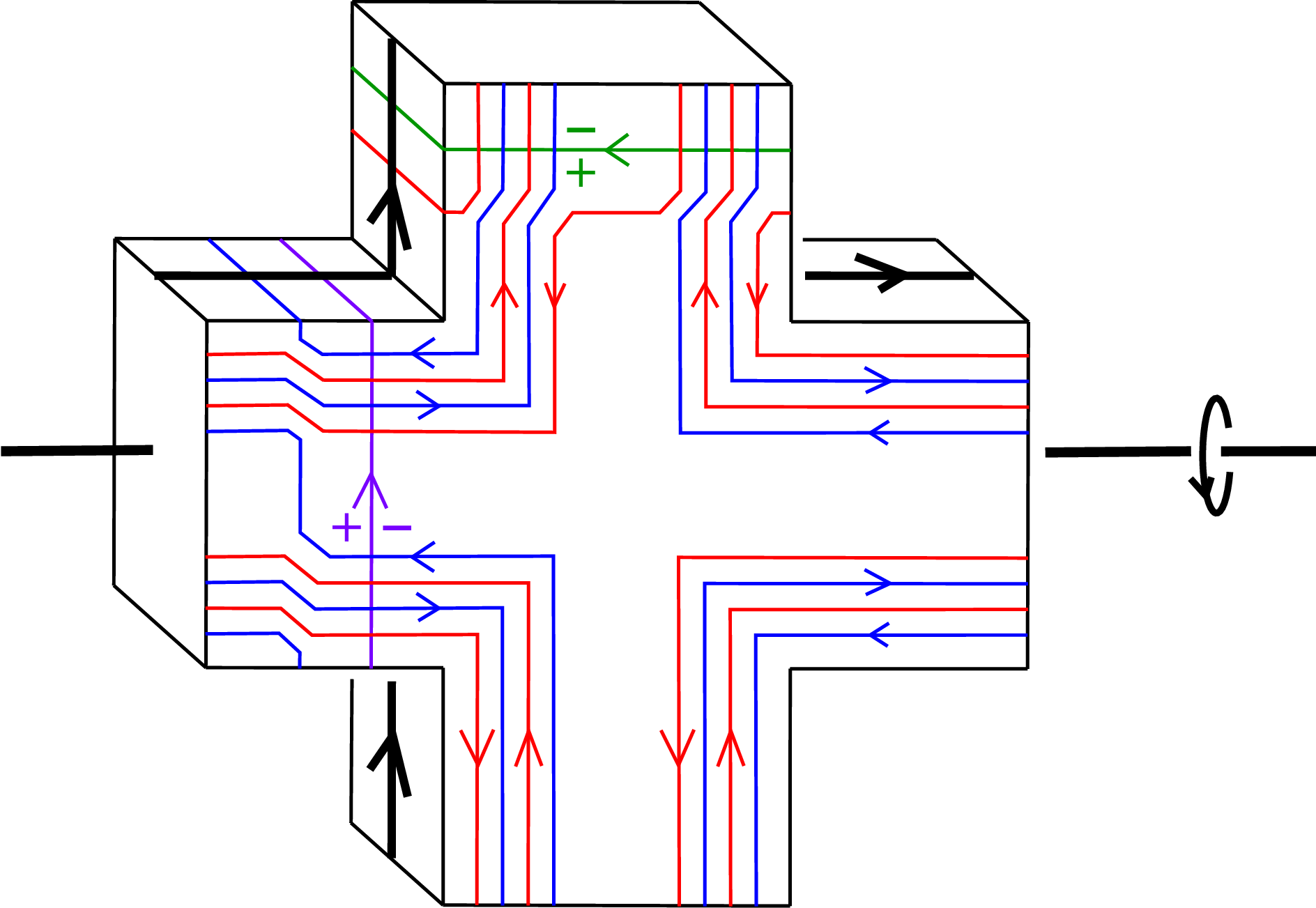
6.4 A presentation of
Since every element of fixes the binding as a set and the element reversing the binding, is generated by the element of and . Moreover, since is a normal subgroup of and , we see that . We give a presentation of and consider the conjugate action of .
6.4.1 A presentation of
Since every element of commutes with the monodromy , we know that by Theorem 1.1. Fix two unoriented simple closed curves and in as in Figure 6. It is known that has a presentation , where and correspond to and , respectively, see the next paragraph of Theorem 3.14 of [9]. Under this presentation, corresponds to . Hence has a presentation .

6.4.2 A conjugate action of
Recall that is , and that is a composition of and for a simple closed curve in . Then we see that and . Hence we conclude that .
References
- [1] E. Akbas. A presentation for the automorphisms of the 3-sphere that preserve a genus two Heegaard splitting. Pacific J. Math. 236 (2008), no. 2, 201–222.
- [2] J. W. Alexander. A lemma on systems of knotted curves. Proceedings of the National Academy of Sciences, 9(3):93–95, 1923.
- [3] S. Cho. Homeomorphisms of the 3-sphere that preserve a Heegaard splitting of genus two. Proc. Amer. Math. Soc. 136 (2008), no. 3, 1113–1123.
- [4] S. Cho. Genus two Goeritz groups of lens spaces. Pacific J.Math. 265 (2013), no. 1, 1–16.
- [5] S. Cho, Y. Koda. The genus two Goeritz group of . Math. Res. Lett. 21 (2014), no. 3, 449–460.
- [6] S. Cho, Y. Koda. Disk complexes and genus two Heegaard splittings for non-prime 3-manifolds. Int. Math. Res. Not. IMRN 2015 (2015), 4344–4371.
- [7] S. Cho, Y. Koda. Connected primitive disk complexes and genus two Goeritz groups of lens spaces. Int. Math. Res. Not. IMRN 2016 (2016), 7302–7340.
- [8] S. Cho, Y. Koda. The mapping class groups of reducible Heegaard splittings of genus two. Transactions of American Mathematical Society 371 (2019), no. 4, 2473–2502.
- [9] B. Farb, D. Margalit. A primer on mapping class groups, Princeton Mathematical Series, 49. Princeton University Press, Princeton, NJ, 2012.
- [10] M. Freedman, M. Scharlemann. Powell moves and the Goeritz group. arXiv:1804.05909.
- [11] L. Goeritz. Die Abbildungen der Berzelfl’́ache und der Volbrezel vom Gesschlect 2. Abh. Math. Sem. Univ. Hamburg 9 (1933), 244–259.
- [12] J. Hempel. 3-manifolds as viewed from the curve complex. Topology 40 (2001), no. 3, 631–657.
- [13] D. Iguchi. Thick isotopy property and the mapping class groups of Heegaard splittings. arXiv:2008.11548.
- [14] D. Iguchi, Y. Koda. Twisted book decompositions and the Goeritz groups. Topology Appl. 272 (2020), 107064, 15 pp.
- [15] W. Jaco. Lectures on three-manifold topology. CBMS Regional Conference Series in Mathematics, vol. 43, American Mathematical Society, Providence, RI, 1980.
- [16] J. Johnson. Mapping class groups of medium distance Heegaard splittings. Proc. Amer. Math. Soc. 138 (2010), no. 12, 4529–4535.
- [17] J. Johnson. Heegaard splittings and open books. arXiv:1110.2142.
- [18] Y. Moriah, J. Schultens. Irreducible Heegaard splittings of Seifert fibered spaces are either vertical or horizontal. Topology 37 (1998), no. 5, 1089–1112.
- [19] M. Scharlemann. Automorphisms of the 3-sphere that preserve a genus two Heegaard splitting. Bol. Soc. Mat. Mexicana (3) 10 (2004), Special Issue, 503–514.
- [20] N. Sekino. Genus one fibered knots in 3-manifolds with reducible genus two Heegaard splittings. Topology Appl. 239 (2018), 46–64.
- [21] N. Sekino. The Goeritz group of a Heegaard splitting of genus two of a Seifert manifold whose base orbifold is sphere with three exceptional points of sufficiently complex coefficients. arXiv:2202.05064.
GRADUATE SCHOOL OF MATHEMATICAL SCIENCES, THE UNIVERSITY OF TOKYO, 3-8-1 KOMABA, MEGURO–KU, TOKYO, 153-8914, JAPAN
E-mail address: sekinonozomu@g.ecc.u-tokyo.ac.jp