跳到论文正文
W Papers独立论文阅读器 arXiv:2203.06973 论文正文 计算阅读时间 · 0%
引用这篇论文根据当前论文元数据生成,正式投稿前建议核对。


License: CC BY 4.0
arXiv:2203.06973v2 [math.NA] 30 Aug 2022

Solving Parametric Partial Differential Equations with Deep Rectified Quadratic Unit Neural Networks

Zhen Lei 11 1 School of Mathematical Sciences; LMNS and Shanghai Key Laboratory for Contemporary Applied Mathematics, Fudan University, Shanghai 200433, P. R. China. 22 2 Email: zlei@fudan.edu.cn    Lei Shi 11footnotemark: 1 33 3 Email: leishi@fudan.edu.cn    Chenyu Zeng 11footnotemark: 1 44 4 Correspondence author. Email: cyzeng19@fudan.edu.cn
August 11, 2026
Abstract

Implementing deep neural networks for learning the solution maps of parametric partial differential equations (PDEs) turns out to be more efficient than using many conventional numerical methods. However, limited theoretical analyses have been conducted on this approach. In this study, we investigate the expressive power of deep rectified quadratic unit (ReQU) neural networks for approximating the solution maps of parametric PDEs. The proposed approach is motivated by the recent important work of G. Kutyniok, P. Petersen, M. Raslan and R. Schneider (Gitta Kutyniok, Philipp Petersen, Mones Raslan, and Reinhold Schneider. A theoretical analysis of deep neural networks and parametric pdes. Constructive Approximation, pages 1-53, 2021), which uses deep rectified linear unit (ReLU) neural networks for solving parametric PDEs. In contrast to the previously established complexity-bound 𝒪⁡(d3​log2q⁡(1/ϵ))\mathcal{O}\left(d^{3}\log_{2}^{q}(1/\epsilon)\right) for ReLU neural networks, we derive an upper bound 𝒪⁡(d3​log2q​log2⁡(1/ϵ))\mathcal{O}\left(d^{3}\log_{2}^{q}\log_{2}(1/\epsilon)\right) on the size of the deep ReQU neural network required to achieve accuracy ϵ>0\epsilon>0, where dd is the dimension of reduced basis representing the solutions. Our method takes full advantage of the inherent low-dimensionality of the solution manifolds and better approximation performance of deep ReQU neural networks. Numerical experiments are performed to verify our theoretical result.

Keywords: Deep neural network; Solution maps of parametric PDE; ReQU activation function; Reduced basis method; Complexity bounds.

1 Introduction

Solving partial differential equations (PDEs) numerically has attracted considerable research attention because of its potential application in many science and engineering problems. Conventional numerical methods, such as finite element and finite difference methods, are primarily used for solving low-dimensional PDEs. In these methods, an equation is solved by discretizing the domain, which could be sufficiently accurate with fine grids. However, conventional methods are often limited by the curse of dimensionality, as they approximate the function values of the solution on grid points which scale exponentially with the input dimension. On the other hand, in most applications, the concerned PDE typically depends on several parameters that describe the physical or geometrical constraints of the equation. Under certain circumstances, PDEs are solved repeatedly for various values of these parameters. Thus, solving PDEs using conventional methods could be time consuming.

Because of the expressive power of neural networks, considerable advancements have been achieved in using deep learning methods for solving PDEs. A flourishing line of research leverages neural networks to approximate the solutions of PDEs directly (see, e.g. [10, 27]), producing efficient numerical methods which outperform the conventional methods in solving high-dimensional PDEs. However, this line of work still aims to build one solution from a parameter set to a state space and thus cannot avoid the trouble of retraining for different parameters. To address this problem, studies ([3, 5, 13, 18, 19]) have proposed the use of neural networks for recovering the solution maps. This approach can be used to solve an entire family of PDEs. However, the theoretical foundations, including the required network size, for this approach have not yet been comprehensively investigated.

In the recent important work [15], the authors have made a significant breakthrough, showing that an efficient approximation of the solution map can be realized using deep neural networks and the low dimensionality of the solution manifold. The following parametric PDEs have been considered:

By​(uy,v)=fy​(v) for all ​y∈𝒴,v∈H,B_{y}(u_{y},v)=f_{y}(v)\quad\text{~for all~}y\in\mathcal{Y},v\in H, (1.1)

where By:H×H→ℝB_{y}:H\times H\to\mathbb{R} is a continuous bilinear form, 𝒴\mathcal{Y} is the set of parameters, and HH is a Hilbert space. The authors of [15] focused on approximating the solution map 𝒴∋y↦uy∈H\mathcal{Y}\ni y\mapsto u_{y}\in H. Based on the Galerkin method and the compactness of parameter set 𝒴\mathcal{Y}, one can assume that there exists a basis of a high-fidelity discretization of HH which may potentially be quite large and the corresponding high-fidelity solutions uyhu^{\mathrm{h}}_{y}. Combined with the reduced basis theory, the high-fidelity space could be replaced by a considerably smaller space of dimension dd, that is, the reduced basis space. And it suffices to approximate the reduced basis solution uyrbu^{\mathrm{rb}}_{y}. In terms of the coefficient vector, this approach transformed the original problem into solving a linear system of equations, which are presented in Section 2.2. The main contribution of [15] is that they constructed a neural network equipped with the rectified linear unit (ReLU) activation function of size 𝒪⁡(d3​log2q⁡(1/ϵ))\mathcal{O}(d^{3}\log^{q}_{2}(1/\epsilon)) to approximate the matrix inversion operator up to accuracy ϵ>0\epsilon>0, where dd is the dimension of reduced basis representing the solutions and the ReLU activation function is defined as x→max⁡{0,x}x\to\max\{0,x\}. Furthermore, they obtained the upper bounds of the complexity of using deep ReLU neural networks for approximating the solution maps of parametric PDEs. Since then, it remains a natural question whether this complexity bound could be further improved when some other neural network architectures are adopted.

In this study, we propose the use of deep neural networks equipped with the rectified quadratic unit (ReQU) activation function to approximate the solution maps of parametric PDEs. Here, ReQU is defined as x→max⁡{0,x2}.x\to\max\{0,x^{2}\}. Compared with the approximation by deep ReLU neural networks, we obtain a better complexity estimate of order 𝒪⁡(d3​log2q​log2⁡(1/ϵ))\mathcal{O}\left(d^{3}\log_{2}^{q}\log_{2}(1/\epsilon)\right) when solving the parametric PDEs with ϵ\epsilon-accuracy using deep ReQU neural networks.

The ReQU is considered as the activation function because as indicated in [17], ReQU neural networks exhibit superior approximation of smooth functions, such as polynomials. This is achieved by the fact that functions x,x2x,x^{2}, and x​yxy can be exactly represented using ReQU neural networks with less nodes and nonzero weights, and without restriction on the norm of xx and yy. Based on these properties, we propose using ReQU neural networks to represent matrix polynomials, which contributes to an approximation of the inversion operator. A key difficulty in implementing our strategy is deriving a ReQU-based neural network calculus. We overcome this problem using a novel construction of identity function and complexity estimates of operations of neural networks equipped with the ReQU activation function.

Furthermore, another important ingredient of our study is the inherent low dimensionality of the solution manifold. This forms the foundation of reduced basis method [12, 15, 24], where the parameter-dependent solutions are obtained in a low-dimensional space constructed using the snapshots of high-dimensional discrete solutions for selected parameters. Typically, this reduced space is built up in advance in a costly offline phase, and is suited to approximate all solutions for parameters stemming from a given parameter domain during the so-called online phase. We refer to [24] for an extensive survey of works on reduced basis methods.

Numerous theoretical analysis based on neural networks have been proposed for solving parametric PDEs. The work [26] was one of the first to present a method for analyzing neural network approximation rates for solutions of parametric PDEs. In their approach, the analyticity of the solution map and polynomial chaos expansion were used to approximate the solution map. In [14, 16], detailed error estimates of neural networks were obtained for Fourier neural operators and DeepONets. We also mention that ReQU neural networks have already been used in [4, 20, 21]) to provide a theoretical upper bound on deep neural network function approximations, which was improved by [17, 28] for smooth functions and in [22] for holomorphic maps in high dimension. The ReQU neural network has been adapted to solve PDEs in [6, 11]. To the best of our knowledge, this study is the first to use ReQU neural networks for solving parametric PDEs.

The rest of this paper is organized as follows. In Section 2, we present the framework of the parametric PDEs problem, and briefly describe the theory of reduced basis method and rectified power units (RePU) activation function. In Section 3, we introduce the ReQU-based neural network calculus, which is the basis for assembling complex neural networks. In Section 4, we construct the ReQU neural network for mapping a matrix to its approximate inverse, and prove its upper bound of complexity. We describe the final approximate solution to parametric PDEs constructed by ReQU neural networks and the corresponding complexity estimates in Section 5. In Section 6, we detail some numerical experiments to support the theoretical analysis results.

2 Preliminary

2.1 Well-Posedness Theory of Parametric PDEs

This subsection introduces the assumptions that guarantee the well-posedness of parametric PDEs. The parametric PDEs are given in (1.1) with a continuous bilinear form By:H×H→ℝB_{y}:H\times H\to\mathbb{R} and a set of parameters denoted by 𝒴.\mathcal{Y}. Here, HH is a Hilbert space with norm ∥⋅∥H\|\cdot\|_{H}, and 𝒴\mathcal{Y} is a compact subset of ℝp\mathbb{R}^{p} with a fixed, but potentially large, p∈ℕp\in\mathbb{N}.

Assumption 2.1.

The bilinear form ByB_{y} satisfies the following conditions:

  1. (i)

    By​(u,v)=By​(v,u), for all ​u,v∈H,y∈𝒴.B_{y}(u,v)=B_{y}(v,u),\quad\text{ for all }u,v\in H,y\in\mathcal{Y}.

  2. (ii)

    There exists a constant α>0\alpha>0 such that

    |By​(u,v)|≤α​‖u‖H​‖v‖H, for all ​u∈H,v∈H,y∈𝒴.\left|B_{y}(u,v)\right|\leq\alpha\|u\|_{H}\|v\|_{H},\quad\text{ for all }u\in H,v\in H,y\in\mathcal{Y}.
  3. (iii)

    There exists a constant β>0\beta>0 such that

    By​(u,u)≥β​‖u‖H2, for all ​u∈H,y∈𝒴.B_{y}(u,u)\geq\beta\|u\|_{H}^{2},\quad\text{ for all }u\in H,y\in\mathcal{Y}.

Moreover, we assume that there exists a constant Cf>0C_{f}>0 such that

‖fy‖H≤Cf, for all ​y∈𝒴,\left\|f_{y}\right\|_{H}\leq C_{f},\quad\text{ for all }y\in\mathcal{Y},

and the solution manifold

S(𝒴):={uy:uy is the solution of (1.1),y∈𝒴}S(\mathcal{Y}):=\left\{u_{y}:u_{y}\text{ is the solution of }\eqref{PPDE},y\in\mathcal{Y}\right\}

is compact in HH.

Next, based on the Lax–Milgram lemma [8], the parametric PDE (1.1) is well-posed; that is, for every y∈𝒴y\in\mathcal{Y} and every fy∈Hf_{y}\in H, there exists exactly one uy∈Hu_{y}\in H such that (1.1) is satisfied, and uyu_{y} depends continuously on fyf_{y}.

Parametric PDEs of form (1.1) are widely used throughout engineering and applied sciences as models for unsteady and steady heat and mass transfer, acoustics, solid and fluid mechanics, electromagnetics, or finance problems [12]. The parameters in 𝒴\mathcal{Y} are used to characterize a particular equation and possible variations in its geometric configuration, physical properties, boundary conditions, or source terms.

Typical examples of parametric PDEs include the boundary-value problem of linear parametric elliptic PDE with variable coefficients

{−∑i,j=1n(ayi​j(x)uxi)xj+∑i=1nbyi(x)uxi+cy(x)u=fy, in ​U,u=0 on ​∂U,\displaystyle\begin{cases}-\sum_{i,j=1}^{n}\left(a_{y}^{ij}(x)u_{x_{i}}\right)_{x_{j}}+\sum_{i=1}^{n}b_{y}^{i}(x)u_{x_{i}}+c_{y}(x)u=f_{y},&\text{~in~}U,\\ u=0&\text{~on~}\partial U,\end{cases} (2.1)

where UU is an open bounded subset of ℝn\mathbb{R}^{n}. We assume that, for every fixed y∈𝒴y\in\mathcal{Y}, there exists a constant θy>0\theta_{y}>0 such that

∑i,j=1nayi​j​(x)​ξi​ξj≥θy​|ξ|2\sum_{i,j=1}^{n}a_{y}^{ij}(x)\xi_{i}\xi_{j}\geq\theta_{y}|\xi|^{2}

for a.e. x∈Ux\in U and all ξ∈ℝn\xi\in\mathbb{R}^{n}. The bilinear form ByB_{y} associated with (2.1) is expressed as follows:

By​(u,v):=∫U∑i,j=1nayi​j​uxi​vxj+∑i=1nbyi​uxi​v+cy​u​v​𝑑x\displaystyle B_{y}(u,v):=\int_{U}\sum_{i,j=1}^{n}a_{y}^{ij}u_{x_{i}}v_{x_{j}}+\sum_{i=1}^{n}b_{y}^{i}u_{x_{i}}v+c_{y}uvdx (2.2)

for u,v∈H01​(U)u,v\in H_{0}^{1}(U), which satisfies conditions (i)-(iii) in Assumption 2.1.

2.2 Reduced Basis Solution

In practice, we cannot solve the equation (1.1) exactly for every y∈𝒴y\in\mathcal{Y}. Instead, we construct a high-fidelity solution uyhu_{y}^{\mathrm{h}} for every fixed yy, which is achieved using the standard Galerkin method, that is, solving (1.1) on a subspace Hm⊂HH_{m}\subset H of dimension mm such that

By​(uym,ei)=fy​(ei) for ​i=1,2,…,m,B_{y}\left(u_{y}^{m},e_{i}\right)=f_{y}(e_{i})\quad\text{ for }i=1,2,\dots,m, (2.3)

where {e1,e2,…,em}\{e_{1},e_{2},\ldots,e_{m}\} is a basis of HmH_{m}, and uymu_{y}^{m} can be represented as uym=∑j=1m(𝐮ym)j​ej.u_{y}^{m}=\sum_{j=1}^{m}\left(\mathbf{u}^{m}_{y}\right)_{j}e_{j}. We denote 𝐁ym:=(By​(ej,ei))i,j=1m∈ℝm×m\mathbf{B}^{m}_{y}:=\left(B_{y}\left(e_{j},e_{i}\right)\right)_{i,j=1}^{m}\in\mathbb{R}^{m\times m} and 𝐟ym:=(fy​(ei))i=1m∈ℝm\mathbf{f}^{m}_{y}:=\left(f_{y}\left(e_{i}\right)\right)_{i=1}^{m}\in\mathbb{R}^{m}, then equation (2.3) is equivalent to the following system of linear equations:

𝐁ym​𝐮ym=𝐟ym,i.e. ​𝐮ym=(𝐁ym)−1​𝐟ym∈ℝm.\mathbf{B}^{m}_{y}\mathbf{u}^{m}_{y}=\mathbf{f}^{m}_{y},\quad\text{i.e.~}\ \mathbf{u}^{m}_{y}=\left(\mathbf{B}^{m}_{y}\right)^{-1}\mathbf{f}^{m}_{y}\in\mathbb{R}^{m}.

Furthermore, based on Céa’s lemma [24], the error uy−uymu_{y}-u_{y}^{m} between the original and Galerkin solution admits the estimate

‖uy−uym‖H≤αβ​infw∈Hm‖uy−w‖H.\left\|u_{y}-u_{y}^{m}\right\|_{H}\leq\frac{\alpha}{\beta}\inf_{w\in H_{m}}\left\|u_{y}-w\right\|_{H}. (2.4)

Thus, because of the compactness of the parametric set 𝒴\mathcal{Y}, we assume that, for an arbitrarily small, but fixed ϵ^>0\hat{\epsilon}>0, there exists a high-fidelity space Hh⊂HH^{h}\subset H with dimension D<D< ∞\infty and basis (ei)i=1D,\left(e_{i}\right)_{i=1}^{D}, such that the corresponding high-fidelity solutions uyhu_{y}^{\mathrm{h}} satisfy

supy∈𝒴‖uy−uyh‖H≤ϵ^.\sup_{y\in\mathcal{Y}}\left\|u_{y}-u_{y}^{\mathrm{h}}\right\|_{H}\leq\hat{\epsilon}.

We denote 𝐁yh:=\mathbf{B}_{y}^{\mathrm{h}}:= (By​(ej,ei))i,j=1D∈ℝD×D\left(B_{y}\left(e_{j},e_{i}\right)\right)_{i,j=1}^{D}\in\mathbb{R}^{D\times D}, 𝐟yh:=(fy​(ei))i=1D\mathbf{f}_{y}^{\mathrm{h}}:=\left(f_{y}\left(e_{i}\right)\right)_{i=1}^{D}, and 𝐮yh:=(𝐁yh)−1​𝐟yh∈ℝD\mathbf{u}_{y}^{\mathrm{h}}:=\left(\mathbf{B}_{y}^{\mathrm{h}}\right)^{-1}\mathbf{f}_{y}^{\mathrm{h}}\in\mathbb{R}^{D}, then we have

uyh:=∑i=1D(𝐮yh)i​ei.u_{y}^{\mathrm{h}}:=\sum_{i=1}^{D}\left(\mathbf{u}_{y}^{\mathrm{h}}\right)_{i}e_{i}.

However, in practice, solving the high-fidelity solution for various parameters entails severe computational costs. Following [15], instead of the high-fidelity solution uyhu_{y}^{\mathrm{h}}, we aim to learn the reduced basis solution uyrbu_{y}^{\mathrm{rb}} of parametric PDE. The reduced basis solution is in a considerably lower dimension space than the high-fidelity solution, while the error between the original solution are comparable. Specifically, we assume that, for every ϵ~≥ϵ^\tilde{\epsilon}\geq\hat{\epsilon}, there exists a reduced basis space Hϵ~rb⊂HH_{\tilde{\epsilon}}^{\mathrm{rb}}\subset H, such that d⁡(ϵ~):=dim⁡(Hϵ~rb)≪Dd(\tilde{\epsilon}):=\operatorname{dim}\left(H_{\tilde{\epsilon}}^{\mathrm{rb}}\right)\ll D and

supy∈𝒴infw∈Hϵ~rb‖uy−w‖H≤ϵ~.\sup_{y\in\mathcal{Y}}\inf_{w\in H_{\tilde{\epsilon}}^{\mathrm{rb}}}\left\|u_{y}-w\right\|_{H}\leq\tilde{\epsilon}. (2.5)

The existence of the reduced basis is based on the compactness of the solution manifold S⁡(𝒴)S(\mathcal{Y}). A detailed discussion is presented in [24].

A basis of Hϵ~rbH_{\tilde{\epsilon}}^{\mathrm{rb}} is constructed from a set of suitable high-fidelity solutions {uy1h,…,uyNh}\left\{u^{\mathrm{h}}_{y^{1}},\ldots,u^{\mathrm{h}}_{y^{N}}\right\} that we call snapshots, corresponding to a set of NN selected parameters 𝒴N={y1,…,yN}⊂𝒴,\mathcal{Y}_{N}=\left\{y^{1},\ldots,y^{N}\right\}\subset\mathcal{Y}, such that

supy∈𝒴infw∈span⁡{uy1h,…,uyNh}‖uy−w‖H≤ϵ~.\sup_{y\in\mathcal{Y}}\inf_{w\in\operatorname{span}\left\{u^{\mathrm{h}}_{y^{1}},\ldots,u^{\mathrm{h}}_{y^{N}}\right\}}\left\|u_{y}-w\right\|_{H}\leq\tilde{\epsilon}.

Next, by orthonormalizing the snapshots, we can generate a set of NN functions {ψ1,…,ψN}\left\{\psi_{1},\ldots,\psi_{N}\right\} called the reduced basis. Through construction, the reduced basis functions are no longer solutions to the high-fidelity problem, but we have

Hϵ~rb:=span⁡{ψ1,…,ψN}=span⁡{uy1h,…,uyNh}H_{\tilde{\epsilon}}^{\mathrm{rb}}:=\operatorname{span}\left\{\psi_{1},\ldots,\psi_{N}\right\}=\operatorname{span}\left\{u^{\mathrm{h}}_{y^{1}},\ldots,u^{\mathrm{h}}_{y^{N}}\right\}

and d⁡(ϵ~):=dim⁡(Hϵ~rb)=N≪D.d(\tilde{\epsilon}):=\operatorname{dim}\left(H_{\tilde{\epsilon}}^{\mathrm{rb}}\right)=N\ll D. The basis vectors (ψi)i=1d⁡(ϵ~)\left(\psi_{i}\right)_{i=1}^{d(\tilde{\epsilon})} are linear combinations of the high-fidelity basis vectors (ei)i=1D\left(e_{i}\right)_{i=1}^{D} with a transformation matrix 𝐕ϵ~∈ℝD×d⁡(ϵ~)\mathbf{V}_{\tilde{\epsilon}}\in\mathbb{R}^{D\times d(\tilde{\epsilon})}, such that

(ψi)i=1d⁡(ϵ~)=(∑j=1D(𝐕ϵ~)j,i​ej)i=1d⁡(ϵ~).\left(\psi_{i}\right)_{i=1}^{d(\tilde{\epsilon})}=\left(\sum_{j=1}^{D}\left(\mathbf{V}_{\tilde{\epsilon}}\right)_{j,i}e_{j}\right)_{i=1}^{d(\tilde{\epsilon})}.

The reduced basis solution can be represented as follows:

uy,ϵ~rb=∑i=1d⁡(ϵ~)(𝐮y,ϵ~rb)i​ψi=∑j=1D(𝐕ϵ~​𝐮y,ϵ~rb)j​ej.u_{y,\tilde{\epsilon}}^{\mathrm{rb}}=\sum_{i=1}^{d(\tilde{\epsilon})}\left(\mathbf{u}_{y,\tilde{\epsilon}}^{\mathrm{rb}}\right)_{i}\psi_{i}=\sum_{j=1}^{D}\left(\mathbf{V}_{\tilde{\epsilon}}\mathbf{u}_{y,\tilde{\epsilon}}^{\mathrm{rb}}\right)_{j}e_{j}. (2.6)

We denote 𝐮~y,ϵ~h:=𝐕ϵ~​𝐮y,ϵ~rb∈ℝD\tilde{\mathbf{u}}_{y,\tilde{\epsilon}}^{\mathrm{h}}:=\mathbf{V}_{\tilde{\epsilon}}\mathbf{u}_{y,\tilde{\epsilon}}^{\mathrm{rb}}\in\mathbb{R}^{D} the coefficient vector of the reduced basis solution if it is expanded with respect to the high-fidelity basis (ei)i=1D.\left(e_{i}\right)_{i=1}^{D}.

Given y∈𝒴y\in\mathcal{Y}, the reduced basis approximation of equation (1.1) is written as follows:

By​(uy,ϵ~rb,v)=fy​(v) for all ​v∈Hϵ~rb.B_{y}\left(u_{y,\tilde{\epsilon}}^{\mathrm{rb}},v\right)=f_{\mathrm{y}}(v)\quad\text{ for all }v\in H_{\tilde{\epsilon}}^{\mathrm{rb}}. (2.7)

By inserting (2.6) into (2.7), we have (see for example [24] Section 3.4.1)

𝐮y,ϵ~rb:=(𝐁y,ϵ~rb)−1​𝐟y,ϵ~rb,\mathbf{u}_{y,\tilde{\epsilon}}^{\mathrm{rb}}:=\left(\mathbf{B}_{y,\tilde{\epsilon}}^{\mathrm{rb}}\right)^{-1}\mathbf{f}_{y,\tilde{\epsilon}}^{\mathrm{rb}}, (2.8)

where

𝐁y,ϵ~rb:=(By​(ψj,ψi))i,j=1d⁡(ϵ~)=𝐕ϵ~T​𝐁yh​𝐕ϵ~∈ℝd⁡(ϵ~)×d⁡(ϵ~), for all ​y∈𝒴\mathbf{B}_{y,\tilde{\epsilon}}^{\mathrm{rb}}:=\left(B_{y}\left(\psi_{j},\psi_{i}\right)\right)_{i,j=1}^{d(\tilde{\epsilon})}=\mathbf{V}_{\tilde{\epsilon}}^{T}\mathbf{B}_{y}^{\mathrm{h}}\mathbf{V}_{\tilde{\epsilon}}\in\mathbb{R}^{d(\tilde{\epsilon})\times d(\tilde{\epsilon})},\quad\text{ for all }y\in\mathcal{Y}

and

𝐟y,ϵ~rb:=(fy​(ψi))i=1d⁡(ε~)=𝐕ϵ~T​𝐟y,ϵ~h∈ℝd⁡(ϵ~).\mathbf{f}_{y,\tilde{\epsilon}}^{\mathrm{rb}}:=\left(f_{y}\left(\psi_{i}\right)\right)_{i=1}^{d(\tilde{\varepsilon})}=\mathbf{V}_{\tilde{\epsilon}}^{T}\mathbf{f}_{y,\tilde{\epsilon}}^{\mathrm{h}}\in\mathbb{R}^{d(\tilde{\epsilon})}.

Then, by using (2.4), we derive the following expression:

supy∈𝒴‖uy−uy,ϵ~rb‖H≤αβ​supy∈𝒴infw∈Hϵ~rb‖uy−w‖H≤αβ​ϵ~.\sup_{y\in\mathcal{Y}}\left\|u_{y}-u_{y,\tilde{\epsilon}}^{\mathrm{rb}}\right\|_{H}\leq\frac{\alpha}{\beta}\sup_{y\in\mathcal{Y}}\inf_{w\in H_{\tilde{\epsilon}}^{\mathrm{rb}}}\left\|u_{y}-w\right\|_{H}\leq\frac{\alpha}{\beta}\tilde{\epsilon}.

Moreover, because bilinear form By​(⋅,⋅)B_{y}(\cdot,\cdot) is symmetric and coercive and the reduced basis functions are orthonormal, we have the following expression:

β≤‖𝐁y,ϵ~rb‖2≤α, as well as α−1≤‖(𝐁y,ϵ~rb)−1‖2≤β−1, for all ​y∈𝒴,\beta\leq\left\|\mathbf{B}_{y,\tilde{\epsilon}}^{\mathrm{rb}}\right\|_{2}\leq\alpha,\quad\text{ as well as }\quad\alpha^{-1}\leq\left\|\left(\mathbf{B}_{y,\tilde{\epsilon}}^{\mathrm{rb}}\right)^{-1}\right\|_{2}\leq\beta^{-1},\quad\text{ for all }y\in\mathcal{Y}, (2.9)

and

|𝐟y,ϵ~rb|≤‖fy‖H≤Cf,\left|\mathbf{f}_{y,\tilde{\epsilon}}^{\mathrm{rb}}\right|\leq\left\|f_{y}\right\|_{H}\leq C_{f},

where |⋅||\cdot| denotes the Euclidean norm, and ∥⋅∥2\|\cdot\|_{2} denotes the spectral norm.

Finally, let 𝐆:=(⟨ei,ej⟩H)i,j=1D∈ℝD×D\mathbf{G}:=\left(\left\langle e_{i},e_{j}\right\rangle_{H}\right)_{i,j=1}^{D}\in\mathbb{R}^{D\times D} be the symmetric, positive definite Gram matrix of the high-fidelity basis (ei)i=1D\left(e_{i}\right)_{i=1}^{D}. Next, for any v∈Hhv\in H_{h} with coefficient vector 𝐯\mathbf{v} with respect to the basis (ei)i=1D\left(e_{i}\right)_{i=1}^{D}, we have the following expression:

|𝐯|𝐆:=|𝐆1/2​𝐯|=‖v‖H.|\mathbf{v}|_{\mathbf{G}}:=\left|\mathbf{G}^{1/2}\mathbf{v}\right|=\|v\|_{H}.

Because the reduced basis functions are orthonormal, we have the following expression:

‖𝐆1/2​𝐕ϵ~‖2=1, for all ​ϵ~≥ϵ^,\left\|\mathbf{G}^{1/2}\mathbf{V}_{\tilde{\epsilon}}\right\|_{2}=1,\quad\text{ for all }\tilde{\epsilon}\geq\hat{\epsilon}, (2.10)

and

‖∑i=1d⁡(ϵ~)𝐜i​ψi‖H=|𝐜|, for all ​𝐜∈ℝd⁡(ϵ~).\left\|\sum_{i=1}^{d(\tilde{\epsilon})}\mathbf{c}_{i}\psi_{i}\right\|_{H}=|\mathbf{c}|,\quad\text{ for all }\mathbf{c}\in\mathbb{R}^{d(\tilde{\epsilon})}.

2.3 Rectified Power Units

In this subsection, we briefly introduce rectified power unit (RePU) activation function, which is the power of the ReLU activation functions. The RePU function is defined as follows:

σs​(x)={xs,x≥0,0,x<0,\sigma_{s}(x)=\begin{cases}x^{s},&x\geq 0,\\ 0,&x<0,\end{cases}

where ss is a non-negative integer. The RePU function with s=1s=1 is the commonly used ReLU function σ1\sigma_{1}. We denote σ2,σ3\sigma_{2},\sigma_{3} ReQU and ReCU for s=2,3s=2,3.

Deep neural networks with the ReLU activation function are becoming increasingly popular because of their high efficiency and versatility. In this study, we performed numerous matrix multiplications based on scalar multiplication and addition. The work [29] has revealed that x2,x​yx^{2},xy can be approximated using a ReLU neural network with depth, the number of weights, and computation units of order 𝒪⁡(log⁡1ϵ)\mathcal{O}(\log\frac{1}{\epsilon}). However, studies have indicated that deep neural networks using RePUs (s≥2s\geq 2 ) as the activation functions exhibit superior approximation property for smooth functions than those using ReLUs [17, 22]. By replacing the ReLU with the RePU(s≥2s\geq 2), the bivariate functions x2x^{2} and x​yxy can be represented with no approximation error using networks with a few nodes and nonzero weights. To be more precise, we introduce the following lemma (see [17])

Lemma 2.2.

For any x,y∈ℝx,y\in\mathbb{R}, the following identities hold

x2=β2T​σ2​(ω2​x),x^{2}=\mathbf{\beta}_{2}^{T}\sigma_{2}\left(\mathbf{\omega}_{2}x\right),
x=β1T​σ2​(ω1​x+γ1),x=\mathbf{\beta}_{1}^{T}\sigma_{2}\left(\mathbf{\omega}_{1}x+\mathbf{\gamma}_{1}\right),
x​y=β1T​σ2​(ω1​x+γ1​y),xy=\mathbf{\beta}_{1}^{T}\sigma_{2}\left(\mathbf{\omega}_{1}x+\mathbf{\gamma}_{1}y\right),

where

β2=[1,1]T,ω2=[1,−1]T,β1=14​[1,1,−1,−1]T,ω1=[1,−1,1,−1]T,γ1=[1,−1,−1,1]T.\mathbf{\beta}_{2}=[1,1]^{T},\mathbf{\omega}_{2}=[1,-1]^{T},\mathbf{\beta}_{1}=\frac{1}{4}[1,1,-1,-1]^{T},\mathbf{\omega}_{1}=[1,-1,1,-1]^{T},\mathbf{\gamma}_{1}=[1,-1,-1,1]^{T}.

and σ2\sigma_{2} acts componentwise.

3 ReQU-Based Neural Network Calculus

3.1 Basic Definitions and Operations

For convenience, we follow the notations of neural networks presented in [7, 15]. Next, we introduce concatenation and parallelization operations for neural networks, which may be used to construct complex neural networks from simple networks. Furthermore, we derive the complexity estimates of operations of ReQU neural networks.

Definition 3.1.

Let n,L∈ℕn,L\in\mathbb{N}. A neural network Φ\Phi with input dimension dimin​(Φ)=n\mathrm{dim}_{\mathrm{in}}(\Phi)=n and number of layers L⁡(Φ)=LL(\Phi)=L is a matrix-vector sequence

Φ=((A1,b1),⋯,(AL,bL)),\Phi=\left(\left(\textbf{A}_{1},\textbf{b}_{1}\right),\cdots,\left(\textbf{A}_{L},\textbf{b}_{L}\right)\right),

where Ak\textbf{A}_{k} are Nk×Nk−1N_{k}\times N_{k-1} matrices, and bk∈ℝNk,N0=n,N1,⋯,NL∈ℕ\textbf{b}_{k}\in\mathbb{R}^{N_{k}},N_{0}=n,N_{1},\cdots,N_{L}\in\mathbb{N}. Let m∈ℕm\in\mathbb{N} and ρ:ℝ→ℝ\rho:\mathbb{R}\rightarrow\mathbb{R} be an arbitrary activation function. We define

Rρ​(Φ):ℝn→ℝNL,Rρ​(Φ)​(x)=xL,\mathrm{R}_{\rho}(\Phi):\mathbb{R}^{n}\rightarrow\mathbb{R}^{N_{L}},\quad R_{\rho}(\Phi)(\textbf{x})=\textbf{x}_{L},

where xL\textbf{x}_{L} is expressed as follows:

{x0:=x,xk:=ρ(Akxk−1+bk),k=1,2,…,L−1,xL:=AL​xL−1+bL,\left\{\begin{array}[]{l}\textbf{x}_{0}:=\textbf{x},\\ \textbf{x}_{k}:=\rho\left(\textbf{A}_{k}\textbf{x}_{k-1}+\textbf{b}_{k}\right),\quad k=1,2,\ldots,L-1,\\ \textbf{x}_{L}:=\textbf{A}_{L}\textbf{x}_{L-1}+\textbf{b}_{L},\end{array}\right.

and

ρ⁡(𝒚):=(ρ⁡(y1),⋯,ρ⁡(ym))T,∀𝒚=(y1,⋯,ym)T∈ℝm.\rho(\boldsymbol{y}):=\left(\rho\left(y^{1}\right),\cdots,\rho\left(y^{m}\right)\right)^{T},\quad\forall\boldsymbol{y}=\left(y^{1},\cdots,y^{m}\right)^{T}\in\mathbb{R}^{m}.

We denote N⁡(Φ):=n+∑k=1LNjN(\Phi):=n+\sum_{k=1}^{L}N_{j} number of nodes, Mk​(Φ):=‖𝐀k‖0+‖𝐛k‖0M_{k}(\Phi):=\left\|\mathbf{A}_{k}\right\|_{0}+\left\|\mathbf{b}_{k}\right\|_{0} the number of nonzero weights in kk-th layer for k≤Lk\leq L and M⁡(Φ):=∑k=1LMk​(Φ)M(\Phi):=\sum_{k=1}^{L}M_{k}(\Phi) the total number of nonzero weights of Φ\Phi. Here, ‖A‖0\left\|\textbf{A}\right\|_{0} denotes the number of nonzero entries of matrix A. We use the number of layers, number of nodes, and number of nonzero weights to measure the complexity of the neural networks.

Next, we define the concatenation of two neural networks as follows:

Definition 3.2.

Let L1,L2∈ℕL_{1},L_{2}\in\mathbb{N} and let Φ1=((A11,b11),…,(AL11,bL11))\Phi^{1}=\left(\left(\textbf{A}_{1}^{1},\textbf{b}_{1}^{1}\right),\ldots,\left(\textbf{A}_{L_{1}}^{1},\textbf{b}_{L_{1}}^{1}\right)\right), Φ2=((A12,b12),…CLOSE\Phi^{2}=\left(\left(\textbf{A}_{1}^{2},\textbf{b}_{1}^{2}\right),\ldots\right., OPEN(AL22,bL22))\left.\left(\textbf{A}_{L_{2}}^{2},\textbf{b}_{L_{2}}^{2}\right)\right) be two neural networks with activation function ρ\rho. The input dimension of Φ1\Phi^{1} is the same as the output dimension of Φ2\Phi^{2}. Next, we denote Φ1∙Φ2\Phi^{1}\bullet\Phi^{2} as the concatenation of Φ1\Phi_{1}, Φ2\Phi_{2} as follows:

Φ1∙Φ2:=((A12,b12),…,(AL2−12,bL2−12),(A11​AL22,A11​bL22+b11),(A21,b21),…,(AL11,bL11)),\Phi^{1}\bullet\Phi^{2}:=\left(\left(\textbf{A}_{1}^{2},\textbf{b}_{1}^{2}\right),\ldots,\left(\textbf{A}_{L_{2}-1}^{2},\textbf{b}_{L_{2}-1}^{2}\right),\left(\textbf{A}_{1}^{1}\textbf{A}_{L_{2}}^{2},\textbf{A}_{1}^{1}\textbf{b}_{L_{2}}^{2}+\textbf{b}_{1}^{1}\right),\left(\textbf{A}_{2}^{1},\textbf{b}_{2}^{1}\right),\ldots,\left(\textbf{A}_{L_{1}}^{1},\textbf{b}_{L_{1}}^{1}\right)\right),

where L⁡(Φ1∙Φ2)=L1+L2−1L(\Phi^{1}\bullet\Phi^{2})=L_{1}+L_{2}-1.

Next, a lemma, which shows that M⁡(Φ1∙Φ2)M\left(\Phi^{1}\bullet\Phi^{2}\right) can be estimated by max⁡{M⁡(Φ1),M⁡(Φ2)}\max\left\{M\left(\Phi^{1}\right),M\left(\Phi^{2}\right)\right\} in some special cases, is presented (see also [15]).

Lemma 3.3.

Let Φ\Phi be a neural network with mm dimensional output and dd dimensional input. If 𝐚∈ℝ1×m\mathbf{a}\in\mathbb{R}^{1\times m}, then, for all k=1,…,L⁡(Φ)k=1,\ldots,L(\Phi),

Mk​(((𝐚,0))∙Φ)≤Mk​(Φ).M_{k}(((\mathbf{a},0))\bullet\Phi)\leq M_{k}(\Phi).

In particular, M⁡((𝐚,0)∙Φ)≤M⁡(Φ).M((\mathbf{a},0)\bullet\Phi)\leq M(\Phi). Moreover, if 𝐃∈ℝd×n\mathbf{D}\in\mathbb{R}^{d\times n} such that, for every k≤dk\leq d there is at most one lk≤nl_{k}\leq n, such that 𝐃k,lk≠0\mathbf{D}_{k,l_{k}}\neq 0, then, for all k=1,…,L⁡(Φ)k=1,\ldots,L(\Phi),

Mk​(Φ∙((𝐃,𝟎ℝd)))≤Mk​(Φ).M_{k}\left(\Phi\bullet\left(\left(\mathbf{D},\mathbf{0}_{\mathbb{R}^{d}}\right)\right)\right)\leq M_{k}(\Phi).

In particular, it holds that M⁡(Φ∙((𝐃,𝟎ℝd)))≤M⁡(Φ)M\left(\Phi\bullet\left(\left(\mathbf{D},\mathbf{0}_{\mathbb{R}^{d}}\right)\right)\right)\leq M(\Phi).

In general, there is no bound on M⁡(Φ1∙Φ2)M\left(\Phi^{1}\bullet\Phi^{2}\right) that is linear in M⁡(Φ1)M\left(\Phi^{1}\right) and M⁡(Φ2)M\left(\Phi^{2}\right). To overcome this problem, we introduce an alternative concatenation to control the number of nonzero weights. Before proceeding, we detail the following lemma, constructing the ReQU neural network of the identity function based on Definition 3.2 and Lemma 2.2. Hereafter, we take σ2\sigma_{2} as the activation function.

Lemma 3.4.

For any n,L∈ℕn,L\in\mathbb{N} and L≥2,L\geq 2, there exists a ReQU neural network Φn,L𝐈𝐝\Phi_{n,L}^{\mathbf{Id}} with n dimensional input and output, satisfying

Rσ2​(Φn,L𝐈𝐝)=𝐈𝐝ℝn\mathrm{R}_{\sigma_{2}}\left(\Phi_{n,L}^{\mathbf{Id}}\right)=\mathbf{Id}_{\mathbb{R}^{n}}

and

M⁡(Φn,L𝐈𝐝)=20​n​L−28​n,M(\Phi_{n,L}^{\mathbf{Id}})=20nL-28n,

where 𝐈𝐝ℝn\mathbf{Id}_{\mathbb{R}^{n}} is identity matrix. Moreover, let ω1=(1,−1,1,−1)T\mathbf{\omega}_{1}=(1,-1,1,-1)^{T}, γ1=(1,−1,1,1)T\mathbf{\gamma}_{1}=(1,-1,1,1)^{T}, β1=14​(1,1,−1,−1)T,\mathbf{\beta}_{1}=\frac{1}{4}(1,1,-1,-1)^{T}, and denote 𝐖∈ℝ4​n×n,𝚪∈ℝ4​n×1,𝐁∈ℝn×4​n\mathbf{W}\in\mathbb{R}^{4n\times n},\mathbf{\Gamma}\in\mathbb{R}^{4n\times 1},\mathbf{B}\in\mathbb{R}^{n\times 4n} as follows :

𝐖:=(ω10⋯00ω1⋯0⋱00⋯ω1),𝚪:=(γ1γ1γ1),𝐁:=(β1T0⋯00β1T⋯0⋱00⋯β1T),\mathbf{W}:=\begin{pmatrix}\mathbf{\omega}_{1}&0&\cdots&0\\ 0&\mathbf{\omega}_{1}&\cdots&0\\ \vdots&\vdots&\ddots&\vdots\\ 0&0&\cdots&\mathbf{\omega}_{1}\end{pmatrix},\ \mathbf{\Gamma}:=\begin{pmatrix}\mathbf{\gamma}_{1}\\ \mathbf{\gamma}_{1}\\ \vdots\\ \mathbf{\gamma}_{1}\end{pmatrix},\ \mathbf{B}:=\begin{pmatrix}\mathbf{\beta}_{1}^{T}&0&\cdots&0\\ 0&\mathbf{\beta}_{1}^{T}&\cdots&0\\ \vdots&\vdots&\ddots&\vdots\\ 0&0&\cdots&\mathbf{\beta}_{1}^{T}\end{pmatrix},

Then Φn,L𝐈𝐝\Phi_{n,L}^{\mathbf{Id}} can be expressed by the following expression:

Φn,L𝐈𝐝=((𝐖,Γ),(𝐖𝐁,Γ),…,(𝐖𝐁,Γ)⏟L−2​ times ,(𝐁,0)).\Phi_{n,L}^{\mathbf{Id}}=(\left(\mathbf{W},\Gamma\right),\underbrace{\left(\mathbf{WB},\Gamma\right),\ldots,\left(\mathbf{WB},\Gamma\right)}_{L-2\text{ times }},\left(\mathbf{B},0\right)). (3.1)

For L=1L=1, we have the following expression:

Φn,1𝐈𝐝=((𝐈𝐝ℝn,0))\Phi_{n,1}^{\mathbf{Id}}=\left(\left(\mathbf{Id}_{\mathbb{R}^{n}},0\right)\right) (3.2)

and M⁡(Φn,1𝐈𝐝)=nM(\Phi_{n,1}^{\mathbf{Id}})=n.

Proof.

When L = 1, the proof is true. When L∈ℕ∩[2,∞)L\in\mathbb{N}\cap[2,\infty), for every n∈ℕn\in\mathbb{N}, based on (3.1), we have the following expression:

M⁡(Φn,L𝐈𝐝)\displaystyle M(\Phi_{n,L}^{\mathbf{Id}}) =‖𝐖‖0+‖𝚪‖0+‖𝐁‖0+(L−2)​(‖𝐖𝐁‖0+‖𝚪‖0)\displaystyle=\|\mathbf{W}\|_{0}+\|\mathbf{\Gamma}\|_{0}+\|\mathbf{B}\|_{0}+(L-2)(\|\mathbf{WB}\|_{0}+\|\mathbf{\Gamma}\|_{0})
=12​n+(L−2)​(16​n+4​n)\displaystyle=12n+(L-2)(16n+4n)
=20​n​L−28​n.\displaystyle=20nL-28n.

The proof is completed. ∎

The sparse concatenation of two neural networks is introduced below.

Definition 3.5.

Let Φ1\Phi^{1} and Φ2\Phi^{2} be two ReQU neural networks, such that the output dimension of Φ2\Phi^{2} and input dimension of Φ1\Phi^{1} equal nn. We define the sparse concatenation of Φ1\Phi^{1} and Φ2\Phi^{2} as

Φ1⊙Φ2:=Φ1∙Φn,2𝐈𝐝∙Φ2.\Phi^{1}\odot\Phi^{2}:=\Phi^{1}\bullet\Phi_{n,2}^{\mathbf{Id}}\bullet\Phi^{2}.

We now introduce another operation, which we call parallelization.

Definition 3.6.

Let Φ1,…,Φk\Phi^{1},\ldots,\Phi^{k} be neural networks that have equal input dimension, such that Φi=((𝐀1i,𝐛1i),…,(𝐀Li,𝐛Li))\Phi^{i}=\left(\left(\mathbf{A}_{1}^{i},\mathbf{b}_{1}^{i}\right),\ldots,\left(\mathbf{A}_{L}^{i},\mathbf{b}_{L}^{i}\right)\right) holds for some L∈ℕ.L\in\mathbb{N}. Next, we define the parallelization of Φ1,…,Φk\Phi^{1},\ldots,\Phi^{k} with

P⁡(Φ1,…,Φk):=(((𝐀110⋯00𝐀12⋯0⋮⋮⋱⋮00⋯𝐀1k),(𝐛11𝐛12⋮𝐛1k)),…,((𝐀L10⋯00𝐀L2⋯0⋮⋮⋱⋮00⋯𝐀Lk),(𝐛L1𝐛L2⋮𝐛Lk))).\mathrm{P}\left(\Phi^{1},\ldots,\Phi^{k}\right):=\left(\left(\left(\begin{array}[]{cccc}\mathbf{A}_{1}^{1}&0&\cdots&0\\ 0&\mathbf{A}_{1}^{2}&\cdots&0\\ \vdots&\vdots&\ddots&\vdots\\ 0&0&\cdots&\mathbf{A}_{1}^{k}\end{array}\right),\left(\begin{array}[]{c}\mathbf{b}_{1}^{1}\\ \mathbf{b}_{1}^{2}\\ \vdots\\ \mathbf{b}_{1}^{k}\end{array}\right)\right),\ldots,\left(\left(\begin{array}[]{cccc}\mathbf{A}_{L}^{1}&0&\cdots&0\\ 0&\mathbf{A}_{L}^{2}&\cdots&0\\ \vdots&\vdots&\ddots&\vdots\\ 0&0&\cdots&\mathbf{A}_{L}^{k}\end{array}\right),\left(\begin{array}[]{c}\mathbf{b}_{L}^{1}\\ \mathbf{b}_{L}^{2}\\ \vdots\\ \mathbf{b}_{L}^{k}\end{array}\right)\right)\right). (3.3)

Now, let Φ\Phi be a neural network and L∈ℕL\in\mathbb{N} such that L⁡(Φ)≤L.L(\Phi)\leq L. Next, define the neural network

EL​(Φ):={Φ, if ​L​(Φ)=L,Φdimout ⁡(Φ),L−L⁡(Φ)𝐈𝐝⊙Φ, if ​L​(Φ)<L.E_{L}(\Phi):=\left\{\begin{array}[]{ll}\Phi,&\text{ if }L(\Phi)=L,\\ \Phi_{\operatorname{dim}_{\text{out }}(\Phi),L-L(\Phi)}^{\mathbf{Id}}\odot\Phi,&\text{ if }L(\Phi)<L.\end{array}\right. (3.4)

Finally, let Φ~1,…,Φ~k\tilde{\Phi}^{1},\ldots,\tilde{\Phi}^{k} be neural networks that have the same input dimension, and let

L~:=max⁡{L⁡(Φ~1),…,L⁡(Φ~k)}.\tilde{L}:=\max\left\{L\left(\tilde{\Phi}^{1}\right),\ldots,L\left(\tilde{\Phi}^{k}\right)\right\}.

Next, we define

P⁡(Φ~1,…,Φ~k):=P⁡(EL~​(Φ~1),…,EL~​(Φ~k)).\mathrm{P}\left(\tilde{\Phi}^{1},\ldots,\tilde{\Phi}^{k}\right):=\mathrm{P}\left(E_{\tilde{L}}\left(\tilde{\Phi}^{1}\right),\ldots,E_{\tilde{L}}\left(\tilde{\Phi}^{k}\right)\right). (3.5)

We call P⁡(Φ~1,…,Φ~k)\mathrm{P}\left(\tilde{\Phi}^{1},\ldots,\tilde{\Phi}^{k}\right) the parallelization of Φ~1,…,Φ~k\tilde{\Phi}^{1},\ldots,\tilde{\Phi}^{k}.

The following two lemmas provide the properties of the sparse concatenation and the parallelization of neural networks.

Lemma 3.7.

Let Φ1,Φ2\Phi^{1},\Phi^{2} be ReQU neural networks. The input dimension of Φ1\Phi^{1} equals the output dimension of Φ2\Phi^{2}, then, for the neural network Φ1⊙Φ2\Phi^{1}\odot\Phi^{2} it holds

  1. (i)

    [Rσ2​(Φ1)∘Rσ2​(Φ2)]​(x)=[Rσ2​(Φ1⊙Φ2)]​(𝐱),[\mathrm{R}_{\sigma_{2}}\left(\Phi^{1}\right)\circ\mathrm{R}_{\sigma_{2}}\left(\Phi^{2}\right)](\textbf{x})=[\mathrm{R}_{\sigma_{2}}\left(\Phi^{1}\odot\Phi^{2}\right)](\mathbf{x}), for every x∈ℝdimin​(Φ2)\textbf{x}\in\mathbb{R}^{\mathrm{dim}_{\mathrm{in}}\left(\Phi^{2}\right)},

  2. (ii)

    L⁡(Φ1⊙Φ2)=L⁡(Φ1)+L⁡(Φ2)L\left(\Phi^{1}\odot\Phi^{2}\right)=L\left(\Phi^{1}\right)+L\left(\Phi^{2}\right),

  3. (iii)

    M⁡(Φ1⊙Φ2)≤M⁡(Φ1)+M⁡(Φ2)+4​M1​(Φ1)+4​ML⁡(Φ2)​(Φ2)+4​dimout​(Φ2)≤5​M​(Φ1)+5​M​(Φ2)+4​dimout​(Φ2),M\left(\Phi^{1}\odot\Phi^{2}\right)\leq M\left(\Phi^{1}\right)+M\left(\Phi^{2}\right)+4M_{1}\left(\Phi^{1}\right)+4M_{L\left(\Phi^{2}\right)}\left(\Phi^{2}\right)+4\mathrm{dim}_{\mathrm{out}}(\Phi^{2})\leq 5M\left(\Phi^{1}\right)+5M\left(\Phi^{2}\right)+4\mathrm{dim}_{\mathrm{out}}(\Phi^{2}),

  4. (iv)

    M1​(Φ1⊙Φ2)=M1​(Φ2)M_{1}\left(\Phi^{1}\odot\Phi^{2}\right)=M_{1}\left(\Phi^{2}\right), if L⁡(Φ2)≥2L(\Phi_{2})\geq 2,

  5. (v)

    ML⁡(Φ1⊙Φ2)​(Φ1⊙Φ2)=ML⁡(Φ1)​(Φ1)M_{L\left(\Phi^{1}\odot\Phi^{2}\right)}\left(\Phi^{1}\odot\Phi^{2}\right)=M_{L\left(\Phi^{1}\right)}\left(\Phi^{1}\right), if L⁡(Φ2)≥2L(\Phi_{2})\geq 2.

Proof.

For every i∈{1,2}i\in\{1,2\}, let Li,N1i,N2i,…,NLii∈ℕ,(𝐀ki,𝐛ki)∈ℝNki×Nk−1i×ℝNki,k∈L_{i},N_{1}^{i},N_{2}^{i},\ldots,N_{L_{i}}^{i}\in\mathbb{N},\left(\mathbf{A}_{k}^{i},\mathbf{b}_{k}^{i}\right)\in\mathbb{R}^{N_{k}^{i}\times N_{k-1}^{i}}\times\mathbb{R}^{N_{k}^{i}},k\in {1,2,…,Li}\left\{1,2,\ldots,L_{i}\right\}, such that

Φi=((𝐀1i,𝐛1i),…,(𝐀Lii,𝐛Lii)).\Phi^{i}=\left(\left(\mathbf{A}_{1}^{i},\mathbf{b}_{1}^{i}\right),\ldots,\left(\mathbf{A}_{L_{i}}^{i},\mathbf{b}_{L_{i}}^{i}\right)\right).

For k∈{1,2,…,L1+L2}k\in\left\{1,2,\ldots,L_{1}+L_{2}\right\}, let (𝐀k,𝐛k)∈ℝNk×Nk−1×ℝNk\left(\mathbf{A}_{k},\mathbf{b}_{k}\right)\in\mathbb{R}^{N_{k}\times N_{k-1}}\times\mathbb{R}^{N_{k}} be the matrix-vector tuples that satisfy

Φ1⊙Φ2=((𝐀1,𝐛1),…,(𝐀L1+L2,𝐛L1+L2)).\Phi^{1}\odot\Phi^{2}=\left(\left(\mathbf{A}_{1},\mathbf{b}_{1}\right),\ldots,\left(\mathbf{A}_{L_{1}+L_{2}},\mathbf{b}_{L_{1}+L_{2}}\right)\right).

Furthermore, for every 𝐱∈ℝN0\mathbf{x}\in\mathbb{R}^{N_{0}}, let 𝐱k\mathbf{x}_{k} be expressed as follows:

𝐱k​(𝐱)={σ2​(𝐀1​𝐱+𝐛1), if ​k=1,σ2​(𝐀k​𝐱k−1​(𝐱)+𝐛k), if ​1<k<L1+L2,𝐀L1+L2​𝐱L1+L2−1​(𝐱)+𝐛L1+L2, if ​k=L1+L2.\mathbf{x}_{k}(\mathbf{x})=\begin{cases}\sigma_{2}\left(\mathbf{A}_{1}\mathbf{x}+\mathbf{b}_{1}\right),&\text{ if }k=1,\\ \sigma_{2}\left(\mathbf{A}_{k}\mathbf{x}_{k-1}(\mathbf{x})+\mathbf{b}_{k}\right),&\text{ if }1<k<L_{1}+L_{2},\\ \mathbf{A}_{L_{1}+L_{2}}\mathbf{x}_{L_{1}+L_{2}-1}(\mathbf{x})+\mathbf{b}_{L_{1}+L_{2}},&\text{ if }k=L_{1}+L_{2}.\end{cases} (3.6)

By definition, we have the following expression:

Φ1⊙Φ2:=((𝐀12,𝐛12),…,(𝐀L2−12,𝐛L2−12),(𝐖𝐀L22,𝐖𝐛L22+𝚪),(𝐀11​𝐁,𝐛11),(𝐀21,𝐛21),…,(𝐀L11,𝐛L11)).\Phi^{1}\odot\Phi^{2}:=\left(\left(\mathbf{A}_{1}^{2},\mathbf{b}_{1}^{2}\right),\ldots,\left(\mathbf{A}_{L_{2}-1}^{2},\mathbf{b}_{L_{2}-1}^{2}\right),\left(\mathbf{W}\mathbf{A}_{L_{2}}^{2},\mathbf{W}\mathbf{b}_{L_{2}}^{2}+\mathbf{\Gamma}\right),\left(\mathbf{A}_{1}^{1}\mathbf{B},\mathbf{b}_{1}^{1}\right),\left(\mathbf{A}_{2}^{1},\mathbf{b}_{2}^{1}\right),\ldots,\left(\mathbf{A}_{L_{1}}^{1},\mathbf{b}_{L_{1}}^{1}\right)\right). (3.7)

For every k∈{1,2,…,L2−1}k\in\left\{1,2,\ldots,L_{2}-1\right\}, (Ak,bk)=(Ak2,bk2).\left(A_{k},b_{k}\right)=\left(A_{k}^{2},b_{k}^{2}\right). This implies that

𝐀L22​𝐱L2−1​(𝐱)+𝐛L22=[Rσ2​(Φ2)]​(𝐱).\mathbf{A}_{L_{2}}^{2}\mathbf{x}_{L_{2}-1}(\mathbf{x})+\mathbf{b}_{L_{2}}^{2}=\left[R_{\sigma_{2}}\left(\Phi^{2}\right)\right](\mathbf{x}). (3.8)

Thus, we have

𝐱L2​(𝐱)=σ2​(AL2​𝐱L2−1​(𝐱)+bL2)=σ2​(𝐖𝐀L22​𝐱L2−1​(𝐱)+(𝐖𝐛L22+𝚪)).\mathbf{x}_{L_{2}}(\mathbf{x})=\sigma_{2}\left(\textbf{A}_{L_{2}}\mathbf{x}_{L_{2}-1}(\mathbf{x})+\textbf{b}_{L_{2}}\right)=\sigma_{2}\left(\mathbf{W}\mathbf{A}_{L_{2}}^{2}\mathbf{x}_{L_{2}-1}(\mathbf{x})+(\mathbf{W}\mathbf{b}_{L_{2}}^{2}+\mathbf{\Gamma})\right). (3.9)

Next (3.7),(3.8), (3.9), and Lemma 3.4 ensure that, for every 𝐱∈ℝN0\mathbf{x}\in\mathbb{R}^{N_{0}}

𝐱L2+1​(𝐱)\displaystyle\mathbf{x}_{L_{2}+1}(\mathbf{x}) =σ2​(AL2+1​(σ2​(AL2​𝐱L2−1​(𝐱)+bL2))+bL2+1)\displaystyle=\sigma_{2}(\textbf{A}_{L_{2}+1}\left(\sigma_{2}\left(\textbf{A}_{L_{2}}\mathbf{x}_{L_{2}-1}(\mathbf{x})+\textbf{b}_{L_{2}}\right)\right)+\textbf{b}_{L_{2}+1})
=σ2​(𝐀11​𝐁​σ2​(𝐖𝐀L22​𝐱L2−1​(𝐱)+(𝐖𝐛L22+𝚪))+𝐛11)\displaystyle=\sigma_{2}(\mathbf{A}_{1}^{1}\mathbf{B}\sigma_{2}\left(\mathbf{W}\mathbf{A}_{L_{2}}^{2}\mathbf{x}_{L_{2}-1}(\mathbf{x})+(\mathbf{W}\mathbf{b}_{L_{2}}^{2}+\mathbf{\Gamma})\right)+\mathbf{b}_{1}^{1})
=σ2​(𝐀11​𝐁​σ2​(𝐖⁡[Rσ2​(Φ2)]​(𝐱)+𝚪)+𝐛11)\displaystyle=\sigma_{2}(\mathbf{A}_{1}^{1}\mathbf{B}\sigma_{2}(\mathbf{W}\left[R_{\sigma_{2}}\left(\Phi^{2}\right)\right](\mathbf{x})+\mathbf{\Gamma})+\mathbf{b}_{1}^{1})
=σ2​(𝐀11​[Rσ2​(Φ2)]​(𝐱)+𝐛11)\displaystyle=\sigma_{2}(\mathbf{A}_{1}^{1}\left[R_{\sigma_{2}}\left(\Phi^{2}\right)\right](\mathbf{x})+\mathbf{b}_{1}^{1})

holds. Combining this with (3.6), we obtain (i). Moreover, (ii), (iv), and (v) follow directly from (3.7).

To prove (iii), note that

ML2​(Φ1⊙Φ2)≤4​ML2​(Φ2)+4​dimout​(Φ2)M_{L_{2}}(\Phi^{1}\odot\Phi^{2})\leq 4M_{L_{2}}(\Phi^{2})+4\mathrm{dim}_{\mathrm{out}}(\Phi^{2})
ML2+1​(Φ1⊙Φ2)≤4​M1​(Φ1),M_{L_{2}+1}(\Phi^{1}\odot\Phi^{2})\leq 4M_{1}(\Phi^{1}),

then, by (3.7) we have

M⁡(Φ1⊙Φ2)\displaystyle M(\Phi^{1}\odot\Phi^{2}) ≤M⁡(Φ1)+M⁡(Φ2)+ML2​(Φ1⊙Φ2)+ML2+1​(Φ1⊙Φ2)\displaystyle\leq M(\Phi^{1})+M(\Phi^{2})+M_{L_{2}}(\Phi^{1}\odot\Phi^{2})+M_{L_{2}+1}(\Phi^{1}\odot\Phi^{2})
≤M⁡(Φ1)+M⁡(Φ2)+4​M1​(Φ1)+4​ML2​(Φ2)+4​d​i​mout​(Φ2).\displaystyle\leq M(\Phi^{1})+M(\Phi^{2})+4M_{1}(\Phi^{1})+4M_{L_{2}}(\Phi^{2})+4\mathrm{dim}_{\mathrm{out}}(\Phi^{2}).

This completes the proof of Lemma 3.7. ∎

Lemma 3.8.

Let Φ1,…,Φk\Phi^{1},\ldots,\Phi^{k} be ReQU neural networks. If the input dimension of Φi\Phi^{i} equals the input dimension of Φj\Phi^{j} for all i,ji,j, then, for the neural network P⁡(Φ1,Φ2,…,Φk)\mathrm{P}\left(\Phi^{1},\Phi^{2},\ldots,\Phi^{k}\right), we have the following expression:

  1. (i)

    Rσ2​(P⁡(Φ1,Φ2,…,Φk))​(𝐱1,…,𝐱k)=(Rσ2​(Φ1)​(𝐱1),Rσ2​(Φ2)​(𝐱2),…,Rσ2​(Φk)​(𝐱k)),\mathrm{R}_{\sigma_{2}}\left(\mathrm{P}\left(\Phi^{1},\Phi^{2},\ldots,\Phi^{k}\right)\right)\left(\mathbf{x}_{1},\ldots,\mathbf{x}_{k}\right)=\left(\mathrm{R}_{\sigma_{2}}\left(\Phi^{1}\right)\left(\mathbf{x}_{1}\right),\mathrm{R}_{\sigma_{2}}\left(\Phi^{2}\right)\left(\mathbf{x}_{2}\right),\ldots,\mathrm{R}_{\sigma_{2}}\left(\Phi^{k}\right)\left(\mathbf{x}_{k}\right)\right), for all 𝐱1,…​𝐱k∈Rn,\mathbf{x}_{1},\ldots\mathbf{x}_{k}\in R^{n},

  2. (ii)

    L⁡(P⁡(Φ1,Φ2,…,Φk))=maxi=1,…,k⁡L⁡(Φi)L\left(\mathrm{P}\left(\Phi^{1},\Phi^{2},\ldots,\Phi^{k}\right)\right)=\max_{i=1,\ldots,k}L\left(\Phi^{i}\right),

  3. (iii)

    M⁡(P⁡(Φ1,Φ2,…,Φk))≤∑i=1k(M⁡(Φi)+4​ML⁡(Φi)​(Φi)+dimout​(Φi)​(20​L​(P⁡(Φ1,Φ2,…,Φk))+8)),M\left(\mathrm{P}\left(\Phi^{1},\Phi^{2},\ldots,\Phi^{k}\right)\right)\leq\sum_{i=1}^{k}\left(M\left(\Phi^{i}\right)+4M_{L\left(\Phi^{i}\right)}\left(\Phi^{i}\right)+\mathrm{dim}_{\mathrm{out}}(\Phi^{i})\big(20L(\mathrm{P}\left(\Phi^{1},\Phi^{2},\ldots,\Phi^{k}\right))+8\big)\right),

  4. (iv)

    M⁡(P⁡(Φ1,Φ2,…,Φk))=∑i=1kM⁡(Φi)M\left(\mathrm{P}\left(\Phi^{1},\Phi^{2},\ldots,\Phi^{k}\right)\right)=\sum_{i=1}^{k}M\left(\Phi^{i}\right), if L⁡(Φ1)=L⁡(Φ2)=…=L⁡(Φk)L\left(\Phi^{1}\right)=L\left(\Phi^{2}\right)=\ldots=L\left(\Phi^{k}\right),

  5. (v)

    M1​(P⁡(Φ1,Φ2,…,Φk))=∑i=1kM1​(Φi),M_{1}\left(\mathrm{P}\left(\Phi^{1},\Phi^{2},\ldots,\Phi^{k}\right)\right)=\sum_{i=1}^{k}M_{1}\left(\Phi^{i}\right),

  6. (vi)

    ML⁡(P⁡(Φ1,Φ2,…,Φk))​(P⁡(Φ1,Φ2,…,Φk))≤∑i=1kmax⁡{4​dimout​(Φi),ML⁡(Φi)​(Φi)},M_{L\left(\mathrm{P}\left(\Phi^{1},\Phi^{2},\ldots,\Phi^{k}\right)\right)}\left(\mathrm{P}\left(\Phi^{1},\Phi^{2},\ldots,\Phi^{k}\right)\right)\leq\sum_{i=1}^{k}\max\left\{4\mathrm{dim}_{\mathrm{out}}\left(\Phi^{i}\right),M_{L\left(\Phi^{i}\right)}\left(\Phi^{i}\right)\right\},

  7. (vii)

    ML⁡(P⁡(Φ1,Φ2,…,Φk))​(P⁡(Φ1,Φ2,…,Φk))=∑i=1kML⁡(Φi)​(Φi)M_{L\left(\mathrm{P}\left(\Phi^{1},\Phi^{2},\ldots,\Phi^{k}\right)\right)}\left(\mathrm{P}\left(\Phi^{1},\Phi^{2},\ldots,\Phi^{k}\right)\right)=\sum_{i=1}^{k}M_{L\left(\Phi^{i}\right)}\left(\Phi^{i}\right), if L⁡(Φ1)=L⁡(Φ2)=…=L⁡(Φk).L\left(\Phi^{1}\right)=L\left(\Phi^{2}\right)=\ldots=L\left(\Phi^{k}\right).

Proof.

By Lemma 3.7, for every i∈{1,2,…,n}i\in\{1,2,\ldots,n\} we have the following expression:

Rσ2​(EL~​(Φi))=Rσ2​(Φi).R_{\sigma_{2}}\left(E_{\tilde{L}}\left(\Phi^{i}\right)\right)=R_{\sigma_{2}}\left(\Phi^{i}\right).

Combining this with (3.4) and (3.5) establishes (i). Furthermore, (ii), (iv), (v), and (vii) follow directly from (3.3), (3.4), and (3.5). In addition, note that (3.1), (3.4), and (3.4) ensure for every i∈{1,2,…,k}i\in\{1,2,\ldots,k\} that

ML⁡(Φ)​(EL⁡(Φ)​(Φi))≤max⁡{4​dimout ⁡(Φi),ML⁡(Φi)​(Φi)},M_{L(\Phi)}\left(E_{L(\Phi)}\left(\Phi^{i}\right)\right)\leq\max\left\{4\operatorname{dim}_{\text{out }}\left(\Phi^{i}\right),M_{L\left(\Phi^{i}\right)}\left(\Phi^{i}\right)\right\},

which implies (v​i).(vi).

Now, we need to show (i​i​i).(iii). Let Φ=P⁡(Φ1,Φ2,…,Φk)\Phi=\mathrm{P}\left(\Phi^{1},\Phi^{2},\ldots,\Phi^{k}\right). By Lemma 3.4, Lemma 3.7, and (3.4), for every i∈{1,2,…,k}i\in\{1,2,\ldots,k\}, if L⁡(Φ)−L⁡(Φi)≥2L(\Phi)-L(\Phi^{i})\geq 2, we have the following expression:

M⁡(EL⁡(Φ)​(Φi))\displaystyle M\left(E_{L(\Phi)}\left(\Phi^{i}\right)\right) ≤M⁡(Φdimout ​(Φi),L⁡(Φ)−L⁡(Φi)Id)+M⁡(Φi)+4​M1​(Φdimout ​(Φi),L⁡(Φ)−L⁡(Φi)Id)\displaystyle\leq M\left(\Phi_{\mathrm{dim}_{\text{out }}(\Phi^{i}),L(\Phi)-L(\Phi^{i})}^{\mathrm{Id}}\right)+M\left(\Phi^{i}\right)+4M_{1}\left(\Phi_{\mathrm{dim}_{\text{out }}(\Phi^{i}),L(\Phi)-L(\Phi^{i})}^{\mathrm{Id}}\right)
+4​ML⁡(Φi)​(Φi)+4​d​i​mout ​(Φi)\displaystyle\quad+4M_{L\left(\Phi^{i}\right)}\left(\Phi^{i}\right)+4\mathrm{dim}_{\text{out }}(\Phi^{i})
≤20​d​i​mout ​(Φi)​L​(Φ)−28​d​i​mout ​(Φi)+M⁡(Φi)+32​d​i​mout ​(Φi)\displaystyle\leq 20\mathrm{dim}_{\text{out }}(\Phi^{i})L(\Phi)-28\mathrm{dim}_{\text{out }}(\Phi^{i})+M(\Phi^{i})+32\mathrm{dim}_{\text{out }}(\Phi^{i})
+4​ML⁡(Φi)​(Φi)+4​d​i​mout ​(Φi)\displaystyle\quad+4M_{L\left(\Phi^{i}\right)}\left(\Phi^{i}\right)+4\mathrm{dim}_{\text{out }}(\Phi^{i})
=M⁡(Φi)+4​ML⁡(Φi)​(Φi)+(20​L​(Φ)+8)​dimout ​(Φi).\displaystyle=M(\Phi^{i})+4M_{L\left(\Phi^{i}\right)}\left(\Phi^{i}\right)+(20L(\Phi)+8)\mathrm{dim}_{\text{out }}(\Phi^{i}). (3.10)

For L⁡(Φ)−L⁡(Φi)=1L(\Phi)-L(\Phi^{i})=1, by Lemma 3.4 and a simple calculation, (3.1) still holds. Combining this with (iv) implies (iii). The proof of Lemma 3.8 is thus completed. ∎

4 Complexity Bound of ReQU Neural Network to Approximate Matrix Inversion

To proceed, we first introduce vectorized matrix hereinafter to stay in the classical neural network setup.

Definition 4.1.

Let 𝐀∈ℝd×l\mathbf{A}\in\mathbb{R}^{d\times l}. We denote

vec⁡(𝐀):=(𝐀1,1,…,𝐀d,1,…,𝐀1,l,…,𝐀d,l)T∈ℝd​l\operatorname{vec}(\mathbf{A}):=\left(\mathbf{A}_{1,1},\ldots,\mathbf{A}_{d,1},\ldots,\mathbf{A}_{1,l},\ldots,\mathbf{A}_{d,l}\right)^{T}\in\mathbb{R}^{dl}

Moreover, for a vector 𝐯=(𝐯1,1,…,𝐯d,1,…,𝐯1,d,…,𝐯d,l)T∈ℝd​l\mathbf{v}=\left(\mathbf{v}_{1,1},\ldots,\mathbf{v}_{d,1},\ldots,\mathbf{v}_{1,d},\ldots,\mathbf{v}_{d,l}\right)^{T}\in\mathbb{R}^{dl}, we set

matr⁡(𝐯):=(𝐯i,j)i=1,…,d,j=1,…,l∈ℝd×l\operatorname{matr}(\mathbf{v}):=\left(\mathbf{v}_{i,j}\right)_{i=1,\ldots,d,j=1,\ldots,l}\in\mathbb{R}^{d\times l}

In this section, we prove the following theorem.

Theorem 4.2.

For ϵ,δ∈(0,1)\epsilon,\delta\in(0,1), we define

l=l⁡(ϵ,δ):=⌈log2⁡(log1−δ⁡(δ​ϵ)+1)⌉,l=l(\epsilon,\delta):=\left\lceil\log_{2}(\log_{1-\delta}(\delta\epsilon)+1)\right\rceil,

where ⌈a⌉:=min⁡{b∈ℤ:b≥a}\lceil a\rceil:=\min\{b\in\mathbb{Z}:b\geq a\} for a∈ℝa\in\mathbb{R}. Let d∈ℕd\in\mathbb{N}, there exists a ReQU neural network Φinv;ϵd\Phi_{\mathrm{inv};\epsilon}^{d} with d2d^{2} dimensional input and d2d^{2} dimensional output satisfying the following properties:

  1. (i)

    sup𝐀∈ℝd×d,‖𝐀‖2≤1−δ‖(𝐈𝐝ℝd−𝐀)−1−matr⁡(Rσ2​(Φinv;ϵd)​(vec⁡(𝐀)))‖2≤ϵ,\sup_{\mathbf{A}\in\mathbb{R}^{d\times d},\|\mathbf{A}\|_{2}\leq 1-\delta}\left\|\left(\mathbf{I}\mathbf{d}_{\mathbb{R}^{d}}-\mathbf{A}\right)^{-1}-\operatorname{matr}\left(\mathrm{R}_{\sigma_{2}}\left(\Phi_{\mathrm{inv};\epsilon}^{d}\right)(\operatorname{vec}(\mathbf{A}))\right)\right\|_{2}\leq\epsilon,

  2. (ii)

    L⁡(Φinv;ϵd)=2​l+1,L\left(\Phi_{\mathrm{inv};\epsilon}^{d}\right)=2l+1,

  3. (iii)

    there exists a universal constant Cinv>0C_{\mathrm{inv}}>0 such that

    M⁡(Φinv;ϵd)≤Cinv​d3​l2.M\left(\Phi_{\mathrm{inv};\epsilon}^{d}\right)\leq C_{\mathrm{inv}}d^{3}l^{2}.

Here, ∥⋅∥2\|\cdot\|_{2} denotes the spectral norm of a matrix. The main purpose of our proof is based on the fact that Neumann series ∑k=0m𝐀k\sum_{k=0}^{m}\mathbf{A}^{k} converges exponentially fast to (𝐈𝐝ℝd−𝐀)−1\left(\mathbf{Id}_{\mathbb{R}^{d}}-\mathbf{A}\right)^{-1} as m→∞m\rightarrow\infty, for 𝐀∈ℝd×d\mathbf{A}\in\mathbb{R}^{d\times d}, satisfying ‖𝐀‖2≤1−δ\|\mathbf{A}\|_{2}\leq 1-\delta for some δ∈(0,1)\delta\in(0,1). To simplify the structure of the ReQU neural network, we consider m=2l−1m=2^{l-1}, and then, factorize polynomial ∑k=02l−1𝐀k=∏k=0l−1(A2k+𝐈𝐝ℝd)\sum_{k=0}^{2^{l}-1}\mathbf{A}^{k}=\prod_{k=0}^{l-1}(\textbf{A}^{2^{k}}+\mathbf{Id}_{\mathbb{R}^{d}}). This reduces the problem to use a neural network to approximate the matrix multiplication.

4.1 ReQU Neural Network to Represent Matrix Multiplication

Proposition 4.3.

Let d,n,l∈ℕ.d,n,l\in\mathbb{N}. There exists a ReQU neural network Φmultd,n,l\Phi_{\mathrm{mult}}^{d,n,l} with n⋅(d+l)n\cdot(d+l) dimensional input and d​ldl dimensional output, such that it satisfies the following properties:

  1. (i)

    matr⁡(Rσ2​(Φmultd,n,l)​(vec⁡(𝐀),vec⁡(𝐁)))=𝐀𝐁,\operatorname{matr}\left(\mathrm{R}_{\sigma_{2}}\left(\Phi_{\mathrm{mult}}^{d,n,l}\right)(\operatorname{vec}(\mathbf{A}),\operatorname{vec}(\mathbf{B}))\right)=\mathbf{AB}, for any 𝐀∈ℝd×n,𝐁∈ℝn×l\mathbf{A}\in\mathbb{R}^{d\times n},\mathbf{B}\in\mathbb{R}^{n\times l},

  2. (ii)

    L⁡(Φmultd,n,l)=2L\left(\Phi_{\mathrm{mult}}^{d,n,l}\right)=2,

  3. (iii)

    M⁡(Φmultd,n,l)≤12​d​n​lM\left(\Phi_{\mathrm{mult}}^{d,n,l}\right)\leq 12dnl,

  4. (iv)

    M1​(Φmultd,n,l)≤8​d​n​l,M_{1}\left(\Phi_{\mathrm{mult}}^{d,n,l}\right)\leq 8dnl,\quad as well as ML⁡(Φmultd,n,l)​(Φmult d,n,l)≤4​d​n​l\quad M_{L\left(\Phi_{\mathrm{mult}}^{d,n,l}\right)}\left(\Phi_{\text{mult }}^{d,n,l}\right)\leq 4dnl.

Proof.

By Lemma 2.2, we can realize scalar multiplication with a ReQU neural network Φ\Phi, satisfying the following equation:

x​y=Rσ2​(Φ)​(x,y)=β1T​σ2​(ω1​x+γ1​y)xy=R_{\sigma_{2}}(\Phi)(x,y)=\mathbf{\beta}_{1}^{T}\sigma_{2}\left(\mathbf{\omega}_{1}x+\mathbf{\gamma}_{1}y\right) (4.1)

and

L⁡(Φ)\displaystyle L\left(\Phi\right) =2,\displaystyle=2, (4.2)
M⁡(Φ)\displaystyle M\left(\Phi\right) ≤12,\displaystyle\leq 12, (4.3)
M1​(Φ)\displaystyle M_{1}\left(\Phi\right) ≤8,\displaystyle\leq 8, (4.4)
ML⁡(Φ)​(Φ)\displaystyle M_{L\left(\Phi\right)}\left(\Phi\right) ≤4.\displaystyle\leq 4. (4.5)

First, for i∈{1,…,d},k∈{1,…,n},j∈{1,…,l}i\in\{1,\ldots,d\},k\in\{1,\ldots,n\},j\in\{1,\ldots,l\}, we define matrix 𝐃i,k,j\mathbf{D}_{i,k,j} such that

𝐃i,k,j​(vec⁡(𝐀),vec⁡(𝐁))=(𝐀i,k,𝐁k,j),∀𝐀∈ℝd×n,𝐁∈ℝn×l,\mathbf{D}_{i,k,j}(\operatorname{vec}(\mathbf{A}),\operatorname{vec}(\mathbf{B}))=\left(\mathbf{A}_{i,k},\mathbf{B}_{k,j}\right),\quad\forall\mathbf{A}\in\mathbb{R}^{d\times n},\mathbf{B}\in\mathbb{R}^{n\times l},

and denote

Φi,k,j:=Φ∙((𝐃i,k,j,𝟎ℝ2)).\Phi_{i,k,j}:=\Phi\bullet\left(\left(\mathbf{D}_{i,k,j},\mathbf{0}_{\mathbb{R}^{2}}\right)\right).

Then, by (4.1), we have the following expression:

𝐀i,k​𝐁k,j=Rσ2​(Φi,k,j)​(vec⁡(𝐀),vec⁡(𝐁))\mathbf{A}_{i,k}\mathbf{B}_{k,j}=\mathrm{R}_{\sigma_{2}}\left(\Phi_{i,k,j}\right)(\operatorname{vec}(\mathbf{A}),\operatorname{vec}(\mathbf{B})) (4.6)

and L⁡(Φi,k,j)=L⁡(Φ)L\left(\Phi_{i,k,j}\right)=L\left(\Phi\right). By Lemma 3.3, Φi,k,j\Phi_{i,k,j} also satisfies (4.3)-(4.5) with Φ\Phi replaced by Φi,j,k\Phi_{i,j,k}.

Next, we define

Φi,j:=((𝟏ℝn,0))∙P⁡(Φi,1,j,…,Φi,n,j)∙(((𝐈𝐝ℝn⁡(d+l)⋮𝐈𝐝ℝn⁡(d+l)),𝟎ℝn2​(d+l))),\Phi_{i,j}:=\left(\left(\mathbf{1}_{\mathbb{R}^{n}},0\right)\right)\bullet\mathrm{P}\left(\Phi_{i,1,j},\ldots,\Phi_{i,n,j}\right)\bullet\left(\left(\left(\begin{array}[]{c}\mathbf{I}\mathbf{d}_{\mathbb{R}^{n(d+l)}}\\ \vdots\\ \mathbf{I}\mathbf{d}_{\mathbb{R}^{n(d+l)}}\end{array}\right),\mathbf{0}_{\mathbb{R}^{n^{2}(d+l)}}\right)\right),

where 𝟏ℝn∈ℝn\mathbf{1}_{\mathbb{R}^{n}}\in\mathbb{R}^{n} is a vector with each entry equal to 1. Next, it follows that Φi,j\Phi_{i,j} is a neural network with n⋅(d+l)n\cdot(d+l) dimensional input and one-dimensional output, satisfying the following expression:

Rσ2​(Φi,j)​(vec⁡(𝐀),vec⁡(𝐁))=∑k=1nRσ2​(Φi,k,j)​(vec⁡(𝐀),vec⁡(𝐁))=∑k=1n𝐀i,k​𝐁k,j.\mathrm{R}_{\sigma_{2}}\left(\Phi_{i,j}\right)(\operatorname{vec}(\mathbf{A}),\operatorname{vec}(\mathbf{B}))=\sum_{k=1}^{n}\mathrm{R}_{\sigma_{2}}\left(\Phi_{i,k,j}\right)(\operatorname{vec}(\mathbf{A}),\operatorname{vec}(\mathbf{B}))=\sum_{k=1}^{n}\mathbf{A}_{i,k}\mathbf{B}_{k,j}. (4.7)

and (4.2) with Φ\Phi replaced by Φi,j\Phi_{i,j}. Moreover, by Lemma 3.3, Lemma 3.8, and (4.3)-(4.5), we obtain the following expression:

M⁡(Φi,j)≤M⁡(P⁡(Φi,1,j,…,Φi,n,j))≤12​n,M\left(\Phi_{i,j}\right)\leq M\left(\mathrm{P}\left(\Phi_{i,1,j},\ldots,\Phi_{i,n,j}\right)\right)\leq 12n, (4.8)
M1​(Φi,j)≤M1​(P⁡(Φi,1,j,…,Φi,n,j))≤8​n,M_{1}\left(\Phi_{i,j}\right)\leq M_{1}\left(\mathrm{P}\left(\Phi_{i,1,j},\ldots,\Phi_{i,n,j}\right)\right)\leq 8n, (4.9)
ML⁡(Φi,j)​(Φi,j)≤ML⁡(Φi,j)​(P⁡(Φi,1,j,…,Φi,n,j))≤4​n.M_{L\left(\Phi_{i,j}\right)}\left(\Phi_{i,j}\right)\leq M_{L\left(\Phi_{i,j}\right)}\left(\mathrm{P}\left(\Phi_{i,1,j},\ldots,\Phi_{i,n,j}\right)\right)\leq 4n. (4.10)

Finally, we define the ReQU neural network Φmultd,n,l\Phi_{\mathrm{mult}}^{d,n,l} with n⋅(d+l)n\cdot(d+l) dimensional input and d​ldl dimensional output as follows:

Φmultd,n,l:=P⁡(Φ1,1,…,Φd,1,…,Φ1,l,…,Φd,l)∙(((𝐈𝐝ℝn⁡(d+l)⋮𝐈𝐝ℝn⁡(d+l)),𝟎ℝd​l​n​(d+l))).\Phi_{\mathrm{mult}}^{d,n,l}:=\mathrm{P}\left(\Phi_{1,1},\ldots,\Phi_{d,1},\ldots,\Phi_{1,l},\ldots,\Phi_{d,l}\right)\bullet\left(\left(\left(\begin{array}[]{c}\mathbf{Id}_{\mathbb{R}^{n(d+l)}}\\ \vdots\\ \mathbf{Id}_{\mathbb{R}^{n(d+l)}}\end{array}\right),\mathbf{0}_{\mathbb{R}^{dln(d+l)}}\right)\right). (4.11)

Then, by (4.7), we have the following expression:

matr⁡(Rσ2​(Φmultd,n,l)​(vec⁡(𝐀),vec⁡(𝐁)))=𝐀𝐁.\operatorname{matr}\left(\mathrm{R}_{\sigma_{2}}\left(\Phi_{\mathrm{mult}}^{d,n,l}\right)(\operatorname{vec}(\mathbf{A}),\operatorname{vec}(\mathbf{B}))\right)=\mathbf{AB}.

By Lemma 3.8, (4.2) is satisfied with Φ\Phi replaced by Φmultd,n,l\Phi_{\mathrm{mult}}^{d,n,l}. Then, by Lemma 3.3, Lemma 3.8, and (4.8), we have the following expression:

M⁡(Φmultd,n,l)≤12​d​n​l.M\left(\Phi_{\mathrm{mult}}^{d,n,l}\right)\leq 12dnl.

Furthermore, by Lemma 3.8, (4.9), and (4.10), we derive

M1​(Φmultd,n,l)≤8​d​n​l​ and ​ML⁡(Φmultd,n,l)​(Φmultd,n,l)≤4​d​n​l.M_{1}\left(\Phi_{\mathrm{mult}}^{d,n,l}\right)\leq 8dnl\text{ and }M_{L\left(\Phi_{\mathrm{mult}}^{d,n,l}\right)}\left(\Phi_{\mathrm{mult}}^{d,n,l}\right)\leq 4dnl.

Thus, we finish the proof. ∎

In particular, let d=n=ld=n=l; then, we have the following corollary.

Corollary 4.4.

Let d∈ℕd\in\mathbb{N}. There exists a ReQU neural network Φmultd,d,d\Phi_{\mathrm{mult}}^{d,d,d} with 2​d22d^{2} dimensional input, d2d^{2} dimensional output such that the following properties are satisfied:

  1. (i)

    matr⁡(Rσ2​(Φmultd,d,d)​(vec⁡(𝐀),vec⁡(𝐁)))=𝐀𝐁\operatorname{matr}\left(\mathrm{R}_{\sigma_{2}}\left(\Phi_{\mathrm{mult}}^{d,d,d}\right)(\operatorname{vec}(\mathbf{A}),\operatorname{vec}(\mathbf{B}))\right)=\mathbf{AB}, for any 𝐀,𝐁∈ℝd×d\mathbf{A},\mathbf{B}\in\mathbb{R}^{d\times d},

  2. (ii)

    L⁡(Φmultd,d,d)=2L\left(\Phi_{\mathrm{mult}}^{d,d,d}\right)=2,

  3. (iii)

    M⁡(Φmultd,d,d)≤12​d3M\left(\Phi_{\mathrm{mult}}^{d,d,d}\right)\leq 12d^{3},

  4. (iv)

    M1​(Φmultd,d,d)≤8​d3,M_{1}\left(\Phi_{\mathrm{mult}}^{d,d,d}\right)\leq 8d^{3},\quad as well as ML⁡(Φmultd,d,d)​(Φmultd,d,d)≤4​d3M_{L\left(\Phi_{\mathrm{mult}}^{d,d,d}\right)}\left(\Phi_{\mathrm{mult}}^{d,d,d}\right)\leq 4d^{3}.

Therefore, we can simulate matrix squaring as follows:

Definition 4.5.

For d∈ℕd\in\mathbb{N}, we define the ReQU neural network

Φ2d:=Φmultd,d,d∙(((𝐈𝐝ℝd2𝐈𝐝ℝd2),𝟎ℝ2​d2)),\Phi_{2}^{d}:=\Phi_{\mathrm{mult}}^{d,d,d}\bullet\left(\left(\left(\begin{array}[]{l}\mathbf{I}\mathbf{d}_{\mathbb{R}^{d^{2}}}\\ \mathbf{I}\mathbf{d}_{\mathbb{R}^{d^{2}}}\end{array}\right),\mathbf{0}_{\mathbb{R}^{2d^{2}}}\right)\right),

which has d2d^{2} dimensional input and d2d^{2} dimensional output.

Then, according to Proposition 4.3, for all d∈ℕd\in\mathbb{N}, we have

Proposition 4.6.

The ReQU neural network Φ2d\Phi_{2}^{d} satisfies the following properties:

  1. (i)

    matr⁡(Rσ2​(Φ2d)​(vec⁡(𝐀)))=𝐀2,\operatorname{matr}\left(\mathrm{R}_{\sigma_{2}}\left(\Phi_{2}^{d}\right)(\operatorname{vec}(\mathbf{A}))\right)=\mathbf{A}^{2}, for any 𝐀∈ℝd×d\mathbf{A}\in\mathbb{R}^{d\times d},

  2. (ii)

    L⁡(Φ2d)=2L\left(\Phi_{2}^{d}\right)=2,

  3. (iii)

    M⁡(Φ2d)≤12​d3,M\left(\Phi_{2}^{d}\right)\leq 12d^{3},

  4. (iv)

    M1​(Φ2d)≤8​d3,M_{1}\left(\Phi_{2}^{d}\right)\leq 8d^{3},\quad as well as ML⁡(Φ2d)​(Φ2d)≤4​d3\quad M_{L\left(\Phi_{2}^{d}\right)}\left(\Phi_{2}^{d}\right)\leq 4d^{3}.

4.2 ReQU Neural Network to Represent the Power Function of the Matrix

Based on the aforementioned results, we can represent map 𝐀↦𝐀2j\mathbf{A}\mapsto\mathbf{A}^{2^{j}} using a ReQU neural network, for arbitrary j∈ℕj\in\mathbb{N}.

Proposition 4.7.

Let d∈ℕ,j∈ℕ.d\in\mathbb{N},j\in\mathbb{N}. There exists a ReQU neural network Φ2jd\Phi_{2^{j}}^{d} with d2d^{2} dimensional input and output that satisfies the following properties:

  1. (i)

    matr⁡(Rσ2​(Φ2jd)​(vec⁡(𝐀)))=𝐀2j,\operatorname{matr}\left(\mathrm{R}_{\sigma_{2}}\left(\Phi_{2^{j}}^{d}\right)(\operatorname{vec}(\mathbf{A}))\right)=\mathbf{A}^{2^{j}}, for any 𝐀∈ℝd×d\mathbf{A}\in\mathbb{R}^{d\times d},

  2. (ii)

    L⁡(Φ2jd)=2​j,L\left(\Phi_{2^{j}}^{d}\right)=2j,

  3. (iii)

    M⁡(Φ2jd)≤64​j​d3,M\left(\Phi_{2^{j}}^{d}\right)\leq 64jd^{3},

  4. (iv)

    M1​(Φ2jd)≤8​d3,M_{1}\left(\Phi_{2^{j}}^{d}\right)\leq 8d^{3},\quad as well as ML⁡(Φ2jd)​(Φ2jd)≤4​d3.\quad M_{L\left(\Phi^{d}_{2^{j}}\right)}\left(\Phi_{2^{j}}^{d}\right)\leq 4d^{3}.

Proof.

We prove the statement by induction. For j=1j=1, the statement proceeds by selecting Φ2d\Phi_{2}^{d} as in Definition 4.5. Next, we assume that the statement holds for an arbitrary, but fixed j∈ℕj\in\mathbb{N}; that is, there exists a neural network Φ2jd\Phi_{2^{j}}^{d} satisfying (i)-(iv). Next, we define the following expression:

Φ2j+1d:=Φ2d⊙Φ2jd.\Phi_{2^{j+1}}^{d}:=\Phi_{2}^{d}\odot\Phi_{2^{j}}^{d}. (4.12)

By inductive hypothesis,

matr⁡(Rσ2​(Φ2j+1d)​(vec⁡(𝐀)))=(matr⁡(Rσ2​(Φ2jd)​(vec⁡(𝐀))))2=𝐀2j+1.\operatorname{matr}\left(\mathrm{R}_{\sigma_{2}}\left(\Phi_{2^{j+1}}^{d}\right)(\operatorname{vec}(\mathbf{A}))\right)=\left(\operatorname{matr}\left(\mathrm{R}_{\sigma_{2}}\left(\Phi_{2^{j}}^{d}\right)(\operatorname{vec}(\mathbf{A}))\right)\right)^{2}=\mathbf{A}^{2^{j+1}}.

We estimate the size of Φ2j+1d\Phi_{2^{j+1}}^{d}. By Lemma 3.7, we obtain the following expression:

L⁡(Φ2j+1d)\displaystyle L\left(\Phi_{2^{j+1}}^{d}\right) =L⁡(Φ2d)+L⁡(Φ2jd)=2+2​j=2​(j+1),\displaystyle=L\left(\Phi_{2}^{d}\right)+L\left(\Phi_{2^{j}}^{d}\right)=2+2j=2(j+1),

and

M⁡(Φ2j+1d)\displaystyle M\left(\Phi_{2^{j+1}}^{d}\right) ≤M⁡(Φ2d)+M⁡(Φ2jd)+4​M1​(Φ2d)+4​ML⁡(Φ2jd)​(Φ2jd)+4​d2\displaystyle\leq M\left(\Phi_{2}^{d}\right)+M\left(\Phi_{2^{j}}^{d}\right)+4M_{1}\left(\Phi_{2}^{d}\right)+4M_{L\left(\Phi_{2^{j}}^{d}\right)}\left(\Phi_{2^{j}}^{d}\right)+4d^{2}
≤12​d3+64​j​d3+4​(4​d3+8​d3)+4​d2\displaystyle\leq 12d^{3}+64jd^{3}+4(4d^{3}+8d^{3})+4d^{2}
≤64​(j+1)​d3.\displaystyle\leq 64(j+1)d^{3}.

Moreover,

M1​(Φ2j+1d)=M1​(Φ2jd)≤8​d3,M_{1}\left(\Phi_{2^{j+1}}^{d}\right)=M_{1}\left(\Phi_{2^{j}}^{d}\right)\leq 8d^{3},
ML⁡(Φ2j+1d)​(Φ2j+1d)=ML⁡(Φ2d)​(Φ2d)≤4​d3.M_{L\left(\Phi_{2^{j+1}}^{d}\right)}\left(\Phi_{2^{j+1}}^{d}\right)=M_{L\left(\Phi_{2}^{d}\right)}\left(\Phi_{2}^{d}\right)\leq 4d^{3}.

The proof is completed. ∎

4.3 Proof of Theorem 4.2

Next, we construct a neural network Φinv;ϵd\Phi_{\mathrm{inv};\epsilon}^{d} that approximates the inversion operator, that is, the map 𝐀↦(𝐈𝐝ℝd−𝐀)−1\mathbf{A}\mapsto\left(\mathbf{I}\mathbf{d}_{\mathbb{R}^{d}}-\mathbf{A}\right)^{-1} up to accuracy ϵ>0\epsilon>0. Based on the properties of the partial sums of the Neumann series, for every ϵ,δ∈(0,1)\epsilon,\delta\in(0,1) and 𝐀∈ℝd×d\mathbf{A}\in\mathbb{R}^{d\times d} satisfying ‖𝐀‖2≤1−δ\|\mathbf{A}\|_{2}\leq 1-\delta, we have the following expression:

‖(𝐈𝐝ℝd−𝐀)−1−∑k=02l−1𝐀k‖2=‖(𝐈𝐝ℝd−𝐀)−1​𝐀2l‖2≤‖(𝐈𝐝ℝd−𝐀)−1‖2​‖𝐀‖22l≤11−(1−δ)⋅(1−δ)2l=(1−δ)2lδ≤ϵ.\begin{aligned} \left\|\left(\mathbf{I}\mathbf{d}_{\mathbb{R}^{d}}-\mathbf{A}\right)^{-1}-\sum_{k=0}^{2^{l}-1}\mathbf{A}^{k}\right\|_{2}&=\left\|\left(\mathbf{I}\mathbf{d}_{\mathbb{R}^{d}}-\mathbf{A}\right)^{-1}\mathbf{A}^{2^{l}}\right\|_{2}\leq\left\|\left(\mathbf{Id}_{\mathbb{R}^{d}}-\mathbf{A}\right)^{-1}\right\|_{2}\|\mathbf{A}\|_{2}^{2^{l}}\\ &\leq\frac{1}{1-(1-\delta)}\cdot(1-\delta)^{2^{l}}=\frac{(1-\delta)^{2^{l}}}{\delta}\leq\epsilon\end{aligned}.

Here, we have used the fact

l⁡(ϵ,δ)=⌈log2⁡(log1−δ⁡(δ​ϵ)+1)⌉≥log2⁡(log1−δ⁡(δ​ϵ)+1).l(\epsilon,\delta)=\left\lceil\log_{2}(\log_{1-\delta}(\delta\epsilon)+1)\right\rceil\geq\log_{2}(\log_{1-\delta}(\delta\epsilon)+1).

Thus, it suffices to construct a ReQU neural network representing ∑k=02l−1𝐀k\sum_{k=0}^{2^{l}-1}\mathbf{A}^{k}. Note that

∑k=02l−1𝐀k=∏i=0l−1(𝐀2i+I);\sum_{k=0}^{2^{l}-1}\mathbf{A}^{k}=\prod_{i=0}^{l-1}(\mathbf{A}^{2^{i}}+I);

by Proposition 4.7 and Corollary 4.4, we have ReQU neural networks Φ2jd\Phi_{2^{j}}^{d} and Φmultd,d,d\Phi_{\mathrm{mult}}^{d,d,d} such that

matr⁡(Rσ2​(Φ2jd)​(vec⁡(𝐀)))=𝐀2j,∀j∈ℕ,\operatorname{matr}\left(\mathrm{R}_{\sigma_{2}}\left(\Phi_{2^{j}}^{d}\right)(\operatorname{vec}(\mathbf{A}))\right)=\mathbf{A}^{2^{j}},\quad\forall j\in\mathbb{N},
matr⁡(Rσ2​(Φmultd,d,d)​(vec⁡(𝐀),vec⁡(𝐁)))=𝐀𝐁.\operatorname{matr}\left(R_{\sigma_{2}}\left(\Phi_{\mathrm{mult}}^{d,d,d}\right)(\operatorname{vec}(\mathbf{A}),\operatorname{vec}(\mathbf{B}))\right)=\mathbf{AB}.

Let b=vec​(𝐈𝐝ℝd2)\textbf{b}=\textbf{vec}(\mathbf{I}\mathbf{d}_{\mathbb{R}^{d^{2}}}) and define Φ1:=((𝐈𝐝ℝd2,b))\Phi_{1}:=((\mathbf{I}\mathbf{d}_{\mathbb{R}^{d^{2}}},\textbf{b})) and

πl:={Φ1,if​l=1,Φmultd,d,d⊙P⁡(πl−1,Φ1⊙Φ2l−1d),if​l≥2.\pi_{l}:=\left\{\begin{array}[]{ll}\Phi_{1},&\text{if}~l=1,\\ \Phi_{\mathrm{mult}}^{d,d,d}\odot P(\pi_{l-1},\Phi_{1}\odot\Phi_{2^{l-1}}^{d}),&\text{if}~l\geq 2.\end{array}\right.

Next, we set

Φinvd:=πl∙(((𝐈𝐝ℝd2⋮𝐈𝐝ℝd2),𝟎ℝl​d2)),\Phi_{\mathrm{inv}}^{d}:=\pi_{l}\bullet\left(\left(\left(\begin{array}[]{c}\mathbf{Id}_{\mathbb{R}^{d^{2}}}\\ \vdots\\ \mathbf{Id}_{\mathbb{R}^{d^{2}}}\end{array}\right),\mathbf{0}_{\mathbb{R}^{ld^{2}}}\right)\right),

which is a ReQU neural network with d2d^{2} dimensional input and output. By the definition of πl\pi_{l}, for every 𝐀∈ℝd×d\mathbf{A}\in\mathbb{R}^{d\times d} such that ‖𝐀‖2≤1−δ\|\mathbf{A}\|_{2}\leq 1-\delta, we have

matr⁡(Rσ2​(Φinvd)​(vec⁡(𝐀)))=∑k=02l−1Ak,\operatorname{matr}\left(\mathrm{R}_{\sigma_{2}}\left(\Phi_{\mathrm{inv}}^{d}\right)(\operatorname{vec}(\mathbf{A}))\right)=\sum_{k=0}^{2^{l}-1}\mathrm{A}^{k},

which implies (i) of Theorem 4.2.

Next, we analyze the size of the resulting neural network Φinvd\Phi_{\mathrm{inv}}^{d}. First, by Lemma 3.7, Lemma 3.8, and Proposition 4.7, we have the following expression:

L⁡(Φinvd)=L⁡(πl)=L⁡(Φmultd,d,d)+max⁡{L⁡(πl−1),L⁡(Φ1⊙Φ2l−1d)}=2+max⁡{L⁡(πl−1),2​l−1}\displaystyle\quad L\left(\Phi_{\mathrm{inv}}^{d}\right)=L(\pi_{l})=L(\Phi_{\mathrm{mult}}^{d,d,d})+\max\{L(\pi_{l-1}),L(\Phi_{1}\odot\Phi_{2^{l-1}}^{d})\}=2+\max\{L(\pi_{l-1}),2l-1\}

Note that L⁡(π2)=5L(\pi_{2})=5, by induction, we have

L⁡(πl)=2​l+1.L(\pi_{l})=2l+1.

For the nonzero weights, we have

M⁡(Φinvd)\displaystyle M\left(\Phi_{\mathrm{inv}}^{d}\right) ≤M⁡(πl)=M⁡(Φmultd,d,d⊙P⁡(πl−1,Φ1⊙Φ2l−1d))\displaystyle\leq M(\pi_{l})=M(\Phi_{\mathrm{mult}}^{d,d,d}\odot P(\pi_{l-1},\Phi_{1}\odot\Phi_{2^{l-1}}^{d})) (4.13)
≤M⁡(Φmultd,d,d)+M⁡(P⁡(πl−1,Φ1⊙Φ2l−1d))\displaystyle\leq M(\Phi_{\mathrm{mult}}^{d,d,d})+M(P(\pi_{l-1},\Phi_{1}\odot\Phi_{2^{l-1}}^{d}))
+4​M1​(Φmultd,d,d)+4​ML⁡(P⁡(πl−1,Φ1⊙Φ2l−1d))​(P⁡(πl−1,Φ1⊙Φ2l−1d))+4​d2\displaystyle+4M_{1}(\Phi_{\mathrm{mult}}^{d,d,d})+4M_{L(P(\pi_{l-1},\Phi_{1}\odot\Phi_{2^{l-1}}^{d}))}(P(\pi_{l-1},\Phi_{1}\odot\Phi_{2^{l-1}}^{d}))+4d^{2}
≤12​d3+M⁡(P⁡(πl−1,Φ1⊙Φ2l−1d))+4×8​d3\displaystyle\leq 12d^{3}+M(P(\pi_{l-1},\Phi_{1}\odot\Phi_{2^{l-1}}^{d}))+4\times 8d^{3}
+4​ML⁡(P⁡(πl−1,Φ1⊙Φ2l−1d))​(P⁡(πl−1,Φ1⊙Φ2l−1d))+4​d2\displaystyle+4M_{L(P(\pi_{l-1},\Phi_{1}\odot\Phi_{2^{l-1}}^{d}))}(P(\pi_{l-1},\Phi_{1}\odot\Phi_{2^{l-1}}^{d}))+4d^{2}
≤44​d3+4​d2+M⁡(P⁡(πl−1,Φ1⊙Φ2l−1d))\displaystyle\leq 44d^{3}+4d^{2}+M(P(\pi_{l-1},\Phi_{1}\odot\Phi_{2^{l-1}}^{d}))
+4​max⁡{4​dimout​(πl−1),ML⁡(πl−1)​(πl−1)}\displaystyle+4\max\{4\mathrm{dim}_{\mathrm{out}}(\pi_{l-1}),M_{L(\pi_{l-1})}(\pi_{l-1})\}
+4​max⁡{4​dimout​(Φ1⊙Φ2l−1d),ML⁡(Φ1⊙Φ2l−1d)​(Φ1⊙Φ2l−1d)}.\displaystyle+4\max\{4\mathrm{dim}_{\mathrm{out}}(\Phi_{1}\odot\Phi^{d}_{2^{l-1}}),M_{L(\Phi_{1}\odot\Phi^{d}_{2^{l-1}})}(\Phi_{1}\odot\Phi^{d}_{2^{l-1}})\}.

Here, by (3.7) and the definition of Φ1\Phi_{1}, we have

ML⁡(Φ1⊙Φ2l−1d)​(Φ1⊙Φ2l−1d)=4​‖𝐈𝐝ℝd2‖0+‖𝐛‖0=4​d2+d2=5​d2,\displaystyle M_{L(\Phi_{1}\odot\Phi^{d}_{2^{l-1}})}(\Phi_{1}\odot\Phi^{d}_{2^{l-1}})=4\|\mathbf{Id}_{\mathbb{R}^{d^{2}}}\|_{0}+\|\mathbf{b}\|_{0}=4d^{2}+d^{2}=5d^{2},

and

max⁡{4​d​i​mout​(Φ1⊙Φ2l−1d),ML⁡(Φ1⊙Φ2l−1d)​(Φ1⊙Φ2l−1d)}=max⁡{4​d2,5​d2}=5​d2.\displaystyle\max\{4\mathrm{dim}_{\mathrm{out}}(\Phi_{1}\odot\Phi^{d}_{2^{l-1}}),M_{L(\Phi_{1}\odot\Phi^{d}_{2^{l-1}})}(\Phi_{1}\odot\Phi^{d}_{2^{l-1}})\}=\max\{4d^{2},5d^{2}\}=5d^{2}. (4.14)

By the definition of πl−1\pi_{l-1}, Lemma 3.7, and Corollary 4.4, we have

max⁡{4​d​i​mout​(πl−1),ML⁡(πl−1)​(πl−1)}=max⁡{4​d2,ML⁡(Φmultd,d,d)​(Φmultd,d,d)}≤4​d3.\displaystyle\max\{4\mathrm{dim}_{\mathrm{out}}(\pi_{l-1}),M_{L(\pi_{l-1})}(\pi_{l-1})\}=\max\{4d^{2},M_{L\left(\Phi_{\mathrm{mult}}^{d,d,d}\right)}\left(\Phi_{\mathrm{mult}}^{d,d,d}\right)\}\leq 4d^{3}. (4.15)

Moreover,

M⁡(P⁡(πl−1,Φ1⊙Φ2l−1d))\displaystyle M(P(\pi_{l-1},\Phi_{1}\odot\Phi_{2^{l-1}}^{d})) (4.16)
≤\displaystyle\leq M⁡(πl−1)+M⁡(Φ1⊙Φ2l−1d)+4​ML⁡(πl−1)​(πl−1)+4​ML⁡(Φ1⊙Φ2l−1Z,d)​(Φ1⊙Φ2l−1d)\displaystyle M(\pi_{l-1})+M(\Phi_{1}\odot\Phi_{2^{l-1}}^{d})+4M_{L(\pi_{l-1})}(\pi_{l-1})+4M_{L(\Phi_{1}\odot\Phi_{2^{l-1}}^{Z,d})}(\Phi_{1}\odot\Phi_{2^{l-1}}^{d})
+dimout ​(πl−1)​(20​L​(πl−1)+8)+dimout​(Φ1⊙Φ2l−1d)​(20​L​(Φ1⊙Φ2l−1d)+8)\displaystyle+\mathrm{dim}_{\text{out }}(\pi_{l-1})(20L(\pi_{l-1})+8)+\mathrm{dim}_{\text{out}}(\Phi_{1}\odot\Phi_{2^{l-1}}^{d})(20L(\Phi_{1}\odot\Phi_{2^{l-1}}^{d})+8)
≤\displaystyle\leq M⁡(πl−1)+(2​d2+64​(l−1)​d3+4×2​d2+4×4​d3+4​d2)+4​(4​d3+5​d2)\displaystyle M(\pi_{l-1})+(2d^{2}+64(l-1)d^{3}+4\times 2d^{2}+4\times 4d^{3}+4d^{2})+4(4d^{3}+5d^{2})
+80​l​d2−24​d2\displaystyle+80ld^{2}-24d^{2}
=\displaystyle= M⁡(πl−1)+64​l​d3−32​d3+80​l​d2+10​d2.\displaystyle M(\pi_{l-1})+64ld^{3}-32d^{3}+80ld^{2}+10d^{2}.

By substituting (4.14)-(4.16) into (4.13), we have

M⁡(πl)\displaystyle M(\pi_{l}) ≤(64​l+28)​d3+(80​l+34)​d2+M⁡(πl−1)\displaystyle\leq(64l+28)d^{3}+(80l+34)d^{2}+M(\pi_{l-1})
≤∑j=2l((64​j+28)​d3+(80​j+34)​d2)+M⁡(π1)\displaystyle\leq\sum_{j=2}^{l}((64j+28)d^{3}+(80j+34)d^{2})+M(\pi_{1})
≤[64​(2+l)​(l−1)2+28​(l−1)]​d3+[80​(2+l)​(l−1)2+34​(l−1)]​d2+2​d2\displaystyle\leq\left[64\frac{(2+l)(l-1)}{2}+28(l-1)\right]d^{3}+\left[80\frac{(2+l)(l-1)}{2}+34(l-1)\right]d^{2}+2d^{2}
=(32​l2+60​l−80)​d3+(40​l2−44​l−112)​d2\displaystyle=(32l^{2}+60l-80)d^{3}+(40l^{2}-44l-112)d^{2}
≤Cinv​d3​l2,\displaystyle\leq C_{\mathrm{inv}}d^{3}l^{2},

where CinvC_{\mathrm{inv}} is a universal constant. The proof is completed.

5 Theoretical Analysis of the ReQU Neural Network to Solve Parametric PDE

In this section, we use ReQU neural networks to approximate the parameter-dependent solution of parametric PDEs, and derive the complexity bounds. As mentioned previously, for any ϵ~≥ϵ^>0\tilde{\epsilon}\geq\hat{\epsilon}>0, there exists reduced basis space Hϵ~rb=span⁡{ψi}i=1d⁡(ϵ~)H_{\tilde{\epsilon}}^{\mathrm{rb}}=\operatorname{span}\{\psi_{i}\}_{i=1}^{d(\tilde{\epsilon})} and corresponding reduced basis solution

uy,ϵ~rb=∑i=1d⁡(ϵ~)(𝐮y,ϵ~rb)i​ψi=∑j=1D(𝐮~y,ϵ~h)j​ej,u_{y,\tilde{\epsilon}}^{\mathrm{rb}}=\sum_{i=1}^{d(\tilde{\epsilon})}\left(\mathbf{u}_{y,\tilde{\epsilon}}^{\mathrm{rb}}\right)_{i}\psi_{i}=\sum_{j=1}^{D}\left(\tilde{\mathbf{u}}^{\mathrm{h}}_{y,\tilde{\epsilon}}\right)_{j}e_{j},

such that

supy∈𝒴‖uy−uy,ϵ~rb‖H≤αβ​ϵ~,\sup_{y\in\mathcal{Y}}\left\|u_{y}-u_{y,\tilde{\epsilon}}^{\mathrm{rb}}\right\|_{H}\leq\frac{\alpha}{\beta}\tilde{\epsilon},

Thus, it suffices to construct ReQU neural networks approximating the maps

𝒴→ℝd⁡(ϵ~):y↦𝐮y,ϵ~rb, and ​𝒴→ℝm:y↦𝐮~y,ϵ~h.\mathcal{Y}\rightarrow\mathbb{R}^{d(\tilde{\epsilon})}:\quad y\mapsto\mathbf{u}_{y,\tilde{\epsilon}}^{\mathrm{rb}},\text{ and }\mathcal{Y}\rightarrow\mathbb{R}^{m}:\quad y\mapsto\tilde{\mathbf{u}}^{\mathrm{h}}_{y,\tilde{\epsilon}}.

Based on the discussion in Section 2, we have the following expression:

𝐮y,ϵ~rb:=(𝐁y,ϵ~rb)−1​𝐟y,ϵ~rb,\mathbf{u}_{y,\tilde{\epsilon}}^{\mathrm{rb}}:=\left(\mathbf{B}_{y,\tilde{\epsilon}}^{\mathrm{rb}}\right)^{-1}\mathbf{f}_{y,\tilde{\epsilon}}^{\mathrm{rb}},

where

𝐁y,ϵ~rb:=(By​(ψj,ψi))i,j=1d⁡(ϵ~),𝐟y,ϵ~rb:=(fy​(ψi))i=1d⁡(ε~) for all ​y∈𝒴.\mathbf{B}_{y,\tilde{\epsilon}}^{\mathrm{rb}}:=\left(B_{y}\left(\psi_{j},\psi_{i}\right)\right)_{i,j=1}^{d(\tilde{\epsilon})},\quad\mathbf{f}_{y,\tilde{\epsilon}}^{\mathrm{rb}}:=\left(f_{y}\left(\psi_{i}\right)\right)_{i=1}^{d(\tilde{\varepsilon})}\quad\text{ for all }y\in\mathcal{Y}.

Our strategy is to first approximate (𝐁y,ϵ~rb)−1(\mathbf{B}_{y,\tilde{\epsilon}}^{\mathrm{rb}})^{-1}, 𝐟y,ϵ~rb\mathbf{f}_{y,\tilde{\epsilon}}^{\mathrm{rb}}, and then, approximate the multiplication of them. By Theorem 4.2, we can approximate (𝐁y,ϵ~rb)−1(\mathbf{B}_{y,\tilde{\epsilon}}^{\mathrm{rb}})^{-1} by applying the neural network Φinv;ϵd\Phi_{\mathrm{inv};\epsilon}^{d} to the matrix 𝐈𝐝ℝd⁡(ϵ~)−λ​𝐁y,ϵ~rb\mathbf{Id}_{\mathbb{R}^{d(\tilde{\epsilon})}}-\lambda\mathbf{B}_{y,\tilde{\epsilon}}^{\mathrm{rb}}. Here, λ\lambda is the scaling factor to ensure ‖𝐈𝐝ℝd⁡(ϵ~)−λ​𝐁y,ϵ~rb‖2<1\left\|\mathbf{Id}_{\mathbb{R}^{d(\tilde{\epsilon})}}-\lambda\mathbf{B}_{y,\tilde{\epsilon}}^{\mathrm{rb}}\right\|_{2}<1. We can select λ:=(α+β)−1\lambda:=\left(\alpha+\beta\right)^{-1} (independent of yy and OPENd⁡(ϵ~))d(\tilde{\epsilon})) such that with δ:=λ​β\delta:=\lambda\beta

‖𝐈𝐝ℝd⁡(ε~)−λ​𝐁y,ϵ~rb‖2=maxμ∈σ⁡(𝐁y,ε~rb)⁡|1−λ​μ|≤maxμ∈[β,α]⁡|1−λ​μ|=1−λ​β=1−δ<1\left\|\mathbf{I}\mathbf{d}_{\mathbb{R}^{d(\tilde{\varepsilon})}}-\lambda\mathbf{B}_{y,\tilde{\epsilon}}^{\mathrm{rb}}\right\|_{2}=\max_{\mu\in\sigma\left(\mathbf{B}_{y,\tilde{\varepsilon}}^{\mathrm{rb}}\right)}|1-\lambda\mu|\leq\max_{\mu\in\left[\beta,\alpha\right]}|1-\lambda\mu|=1-\lambda\beta=1-\delta<1

for all y∈𝒴,ϵ~>0y\in\mathcal{Y},\tilde{\epsilon}>0. We fix these values of λ\lambda and δ\delta for the remainder of this paper. To proceed, we state the assumptions on the approximability of the map 𝐁⋅,ϵ~rb\mathbf{B}_{\cdot,\tilde{\epsilon}}^{\mathrm{rb}} and 𝐟⋅,ϵ~rb\mathbf{f}_{\cdot,\tilde{\epsilon}}^{\mathrm{rb}}.

Assumption 5.1.

For any ϵ~≥ϵ^,ϵ>0\tilde{\epsilon}\geq\hat{\epsilon},\epsilon>0, and a corresponding reduced basis (ψi)i=1d⁡(ϵ~)\left(\psi_{i}\right)_{i=1}^{d(\tilde{\epsilon})}, there exists a neural network Φϵ~,ϵ𝐁\Phi_{\tilde{\epsilon},\epsilon}^{\mathbf{B}} with pp dimensional input and d​(ϵ~)2d(\tilde{\epsilon})^{2} dimensional output such that

supy∈𝒴‖λ​𝐁y,ϵ~rb−matr⁡(Rσ2​(Φϵ~,ϵ𝐁)​(y))‖2≤ϵ.\sup_{y\in\mathcal{Y}}\left\|\lambda\mathbf{B}_{y,\tilde{\epsilon}}^{\mathrm{rb}}-\operatorname{matr}\left(\mathrm{R}_{\sigma_{2}}\left(\Phi_{\tilde{\epsilon},\epsilon}^{\mathbf{B}}\right)(y)\right)\right\|_{2}\leq\epsilon.

We set BL​(ϵ~,ϵ):=L⁡(Φϵ~,ϵ𝐁)B_{L}(\tilde{\epsilon},\epsilon):=L\left(\Phi_{\tilde{\epsilon},\epsilon}^{\mathbf{B}}\right) and BM​(ϵ~,ϵ):=M⁡(Φϵ~,ϵ𝐁)B_{M}(\tilde{\epsilon},\epsilon):=M\left(\Phi_{\tilde{\epsilon},\epsilon}^{\mathbf{B}}\right).

Assumption 5.2.

For every ϵ~≥ϵ^,ϵ>0\tilde{\epsilon}\geq\hat{\epsilon},\epsilon>0, and a corresponding reduced basis (ψi)i=1d⁡(ϵ~)\left(\psi_{i}\right)_{i=1}^{d(\tilde{\epsilon})}, there exists a neural network Φϵ~,ϵ𝐟\Phi_{\tilde{\epsilon},\epsilon}^{\mathbf{f}} with pp dimensional input and d⁡(ϵ~)d(\tilde{\epsilon}) dimensional output such that

supy∈𝒴|𝐟y,ϵ~rb−Rσ2​(Φϵ~,ϵ𝐟)​(y)|≤ϵ.\sup_{y\in\mathcal{Y}}\left|\mathbf{f}_{y,\tilde{\epsilon}}^{\mathrm{rb}}-\mathrm{R}_{\sigma_{2}}\left(\Phi_{\tilde{\epsilon},\epsilon}^{\mathbf{f}}\right)(y)\right|\leq\epsilon.

We set FL​(ϵ~,ϵ):=L⁡(Φϵ~,ϵ𝐟)F_{L}(\tilde{\epsilon},\epsilon):=L\left(\Phi_{\tilde{\epsilon},\epsilon}^{\mathbf{f}}\right) and FM​(ϵ~,ϵ):=M⁡(Φϵ~,ϵ𝐟).F_{M}(\tilde{\epsilon},\epsilon):=M\left(\Phi_{\tilde{\epsilon},\epsilon}^{\mathbf{f}}\right).

Next, we present the construction of the neural network emulating y↦(𝐁y,ϵ~rb)−1y\mapsto\left(\mathbf{B}_{y,\tilde{\epsilon}}^{\mathrm{rb}}\right)^{-1}.

Proposition 5.3.

Let ϵ~≥ϵ^,ϵ>0,\tilde{\epsilon}\geq\hat{\epsilon},\epsilon>0, and ϵ′:=min⁡{3​ϵ​λ​β28,λ​β4}.\epsilon^{\prime}:=\min\{\frac{3\epsilon\lambda\beta^{2}}{8},\frac{\lambda\beta}{4}\}. Under Assumption 5.1, there exists a ReQU neural network Φinv;ϵ~,ϵB\Phi_{\mathrm{inv};\tilde{\epsilon},\epsilon}^{\textbf{B}} with pp dimensional input and d​(ϵ~)2d(\tilde{\epsilon})^{2} dimensional output that satisfies the following properties:

  1. (i)

    supy∈𝒴‖(𝐁y,ϵ~rb)−1−matr⁡(Rσ2​(Φinv;ϵ~,ϵB)​(y))‖2≤ϵ,\sup_{y\in\mathcal{Y}}\left\|\left(\mathbf{B}_{y,\tilde{\epsilon}}^{\mathrm{rb}}\right)^{-1}-\operatorname{matr}\left(\mathrm{R}_{\sigma_{2}}\left(\Phi_{\mathrm{inv};\tilde{\epsilon},\epsilon}^{\textbf{B}}\right)(y)\right)\right\|_{2}\leq\epsilon,

  2. (ii)

    there exists a constant CLB=CLB​(α,β)>0C^{B}_{L}=C^{B}_{L}(\alpha,\beta)>0 such that

    L⁡(Φinv;ϵ~,ϵB)≤CB​log2⁡(log2⁡(1/ϵ))+BL​(ϵ~,ϵ′),L\left(\Phi_{\mathrm{inv};\tilde{\epsilon},\epsilon}^{\textbf{B}}\right)\leq C_{B}\log_{2}(\log_{2}(1/\epsilon))+B_{L}(\tilde{\epsilon},\epsilon^{\prime}),
  3. (iii)

    there exists a constant CMB=CMB​(α,β)>0C^{B}_{M}=C^{B}_{M}(\alpha,\beta)>0 such that

    M⁡(Φinv;ϵ~,ϵB)≤CB​d3​(ϵ~)​log22⁡(log2⁡(1/ϵ))+5​BM​(ϵ~,ϵ′).M\left(\Phi_{\mathrm{inv};\tilde{\epsilon},\epsilon}^{\textbf{B}}\right)\leq C_{B}d^{3}(\tilde{\epsilon})\log^{2}_{2}(\log_{2}(1/\epsilon))+5B_{M}(\tilde{\epsilon},\epsilon^{\prime}).
Proof.

Let ((𝐀ϵ~,ϵ′1,𝐛ϵ~,ϵ′1),…,(𝐀ϵ~,ϵ′L,𝐛ϵ~,ϵ′L)):=Φϵ~,ϵ′𝐁\left(\left(\mathbf{A}_{\tilde{\epsilon},\epsilon^{\prime}}^{1},\mathbf{b}_{\tilde{\epsilon},\epsilon^{\prime}}^{1}\right),\ldots,\left(\mathbf{A}_{\tilde{\epsilon},\epsilon^{\prime}}^{L},\mathbf{b}_{\tilde{\epsilon},\epsilon^{\prime}}^{L}\right)\right):=\Phi_{\tilde{\epsilon},\epsilon^{\prime}}^{\mathbf{B}} be the neural network in Assumption 5.1, then, for

Φϵ~,ϵ′𝐁,𝐈𝐝:=((𝐀ϵ~,ϵ′1,𝐛ϵ~,ϵ′1),…,(−𝐀ϵ~,ϵ′L,−𝐛ϵ~,ϵ′L+vec⁡(𝐈𝐝ℝd⁡(ϵ~)))),\Phi_{\tilde{\epsilon},\epsilon^{\prime}}^{\mathbf{B},\mathbf{Id}}:=\left(\left(\mathbf{A}_{\tilde{\epsilon},\epsilon^{\prime}}^{1},\mathbf{b}_{\tilde{\epsilon},\epsilon^{\prime}}^{1}\right),\ldots,\left(-\mathbf{A}_{\tilde{\epsilon},\epsilon^{\prime}}^{L},-\mathbf{b}_{\tilde{\epsilon},\epsilon^{\prime}}^{L}+\operatorname{vec}\left(\mathbf{I}\mathbf{d}_{\mathbb{R}^{d(\tilde{\epsilon})}}\right)\right)\right),

we have

supy∈𝒴‖𝐈𝐝ℝd⁡(ϵ~)−λ​𝐁y,ϵ~rb−matr⁡(Rσ2​(Φϵ~,ϵ′𝐁,𝐈𝐝)​(y))‖2≤ϵ′,\displaystyle\sup_{y\in\mathcal{Y}}\left\|\mathbf{Id}_{\mathbb{R}^{d(\tilde{\epsilon})}}-\lambda\mathbf{B}_{y,\tilde{\epsilon}}^{\mathrm{rb}}-\operatorname{matr}\left(\mathrm{R}_{\sigma_{2}}\left(\Phi_{\tilde{\epsilon},\epsilon^{\prime}}^{\mathbf{B},\mathbf{Id}}\right)(y)\right)\right\|_{2}\leq\epsilon^{\prime}, (5.1)

as well as M⁡(Φϵ~,ϵ′𝐁,𝐈𝐝)≤BM​(ϵ~,ϵ′)+d2​(ϵ~)M\left(\Phi_{\tilde{\epsilon},\epsilon^{\prime}}^{\mathbf{B},\mathbf{Id}}\right)\leq B_{M}(\tilde{\epsilon},\epsilon^{\prime})+d^{2}(\tilde{\epsilon}) and L⁡(Φϵ~,ϵ′𝐁,𝐈𝐝)=BL​(ϵ~,ϵ′)L\left(\Phi_{\tilde{\epsilon},\epsilon^{\prime}}^{\mathbf{B},\mathbf{Id}}\right)=B_{L}(\tilde{\epsilon},\epsilon^{\prime}). Next, we define the ReQU neural network

Φinv;ϵ~,ϵB:=((λ​𝐈𝐝ℝd⁡(ϵ~),𝟎ℝd⁡(ϵ~)))∙Φinv;ϵ2​λd⁡(ϵ~)⊙Φϵ~,ϵ′𝐁,𝐈𝐝,\Phi_{\mathrm{inv};\tilde{\epsilon},\epsilon}^{\textbf{B}}:=\left(\left(\lambda\mathbf{I}\mathbf{d}_{\mathbb{R}^{d(\tilde{\epsilon})}},\mathbf{0}_{\mathbb{R}^{d(\tilde{\epsilon})}}\right)\right)\bullet\Phi_{\mathrm{inv};\frac{\epsilon}{2\lambda}}^{d(\tilde{\epsilon})}\odot\Phi_{\tilde{\epsilon},\epsilon^{\prime}}^{\mathbf{B},\mathbf{Id}},

with pp dimensional input and d​(ϵ~)2d(\tilde{\epsilon})^{2} dimensional output. To prove (i)(i), it suffices to estimate

‖(λ​𝐁y,ϵ~rb)−1−matr⁡(Rσ2​(Φinv;ϵ2​λd⁡(ϵ~)⊙Φϵ~,ϵ′B,Id)​(y))‖2\displaystyle\left\|\left(\lambda\mathbf{B}_{y,\tilde{\epsilon}}^{\mathrm{rb}}\right)^{-1}-\operatorname{matr}\left(\mathrm{R}_{\sigma_{2}}\left(\Phi_{\mathrm{inv};\frac{\epsilon}{2\lambda}}^{d(\tilde{\epsilon})}\odot\Phi_{\tilde{\epsilon},\epsilon^{\prime}}^{\textbf{B},\textbf{Id}}\right)(y)\right)\right\|_{2} (5.2)
≤\displaystyle\leq ‖(λ​𝐁y,ϵ~rb)−1−(𝐈𝐝ℝd⁡(ϵ~)−matr⁡(Rσ2​(Φϵ~,ϵ′B,Id)​(y)))−1‖2\displaystyle\left\|\left(\lambda\mathbf{B}_{y,\tilde{\epsilon}}^{\mathrm{rb}}\right)^{-1}-\left(\mathbf{Id}_{\mathbb{R}^{d(\tilde{\epsilon})}}-\operatorname{matr}\left(\mathrm{R}_{\sigma_{2}}\left(\Phi_{\tilde{\epsilon},\epsilon^{\prime}}^{\textbf{B},\textbf{Id}}\right)(y)\right)\right)^{-1}\right\|_{2}
+‖(𝐈𝐝ℝd⁡(ϵ~)−matr⁡(Rσ2​(Φϵ~,ϵ′B,Id)​(y)))−1−matr⁡(Rσ2​(Φinv;ϵ2​λd⁡(ϵ~)⊙Φϵ~,ϵ′B,Id)​(y))‖2\displaystyle+\left\|\left(\mathbf{Id}_{\mathbb{R}^{d(\tilde{\epsilon})}}-\operatorname{matr}\left(\mathrm{R}_{\sigma_{2}}\left(\Phi_{\tilde{\epsilon},\epsilon^{\prime}}^{\textbf{B},\textbf{Id}}\right)(y)\right)\right)^{-1}-\operatorname{matr}\left(\mathrm{R}_{\sigma_{2}}\left(\Phi_{\mathrm{inv};\frac{\epsilon}{2\lambda}}^{d(\tilde{\epsilon})}\odot\Phi_{\tilde{\epsilon},\epsilon^{\prime}}^{\textbf{B},\textbf{Id}}\right)(y)\right)\right\|_{2}
=:\displaystyle=: I+II.\displaystyle\mathrm{I}+\mathrm{II}.

For term I\mathrm{I}, by (5.1), we have the following expression:

‖𝐈𝐝ℝd⁡(ϵ~)−matr⁡(Rσ2​(Φϵ~,ϵ′B,Id)​(y))‖2≥‖λ​𝐁y,ϵ~rb‖2−ϵ′≥λ​β−λ​β4=34​λ​β.\displaystyle\left\|\mathbf{Id}_{\mathbb{R}^{d(\tilde{\epsilon})}}-\operatorname{matr}\left(\mathrm{R}_{\sigma_{2}}\left(\Phi_{\tilde{\epsilon},\epsilon^{\prime}}^{\textbf{B},\textbf{Id}}\right)(y)\right)\right\|_{2}\geq\|\lambda\mathbf{B}_{y,\tilde{\epsilon}}^{\mathrm{rb}}\|_{2}-\epsilon^{\prime}\geq\lambda\beta-\frac{\lambda\beta}{4}=\frac{3}{4}\lambda\beta.

By combining Assumption 5.1, (2.9), and (5.2), we obtain

I\displaystyle\mathrm{I} ≤‖(𝐈𝐝ℝd⁡(ϵ~)−matr⁡(Rσ2​(Φϵ~,ϵ′B,Id)​(y)))−1‖2​‖(λ​𝐁y,ϵ~rb)−1‖2​‖𝐈𝐝ℝd⁡(ϵ~)−λ​𝐁y,ϵ~rb−matr⁡(Rσ2​(Φϵ~,ϵ′𝐁,𝐈𝐝)​(y))‖2\displaystyle\leq\left\|\left(\mathbf{Id}_{\mathbb{R}^{d(\tilde{\epsilon})}}-\operatorname{matr}\left(\mathrm{R}_{\sigma_{2}}\left(\Phi_{\tilde{\epsilon},\epsilon^{\prime}}^{\textbf{B},\textbf{Id}}\right)(y)\right)\right)^{-1}\right\|_{2}\left\|\left(\lambda\mathbf{B}_{y,\tilde{\epsilon}}^{\mathrm{rb}}\right)^{-1}\right\|_{2}\left\|\mathbf{Id}_{\mathbb{R}^{d(\tilde{\epsilon})}}-\lambda\mathbf{B}_{y,\tilde{\epsilon}}^{\mathrm{rb}}-\operatorname{matr}\left(\mathrm{R}_{\sigma_{2}}\left(\Phi_{\tilde{\epsilon},\epsilon^{\prime}}^{\mathbf{B},\mathbf{Id}}\right)(y)\right)\right\|_{2}
≤43​1λ​β​1λ​β​ϵ′≤ϵ2​λ.\displaystyle\leq\frac{4}{3}\frac{1}{\lambda\beta}\frac{1}{\lambda\beta}\epsilon^{\prime}\leq\frac{\epsilon}{2\lambda}.

For term II, by the triangle inequality, for every y∈𝒴y\in\mathcal{Y}, we have the following expression:

‖matr⁡(Rσ2​(Φϵ~,ϵ′B,Id)​(y))‖2\displaystyle\left\|\operatorname{matr}\left(\mathrm{R}_{\sigma_{2}}\left(\Phi_{\tilde{\epsilon},\epsilon^{\prime}}^{\textbf{B},\textbf{Id}}\right)(y)\right)\right\|_{2} ≤‖matr⁡(Rσ2​(Φϵ~,ϵ′B,Id)​(y))−(Idℝd⁡(ϵ¯)−λ​𝐁y,ϵ~rb)‖2+‖𝐈𝐝ℝd⁡(ϵ¯)−λ​𝐁y,ϵ~rb‖2\displaystyle\leq\left\|\operatorname{matr}\left(\mathrm{R}_{\sigma_{2}}\left(\Phi_{\tilde{\epsilon},\epsilon^{\prime}}^{\textbf{B},\textbf{Id}}\right)(y)\right)-\left(\textbf{Id}_{\mathbb{R}^{d(\bar{\epsilon})}}-\lambda\mathbf{B}_{y,\tilde{\epsilon}}^{\mathrm{rb}}\right)\right\|_{2}+\left\|\mathbf{Id}_{\mathbb{R}^{d(\bar{\epsilon})}}-\lambda\mathbf{B}_{y,\tilde{\epsilon}}^{\mathrm{rb}}\right\|_{2} (5.3)
≤ϵ′+1−δ≤1−δ+λ​β4≤1−δ+δ2=1−δ2.\displaystyle\leq\epsilon^{\prime}+1-\delta\leq 1-\delta+\frac{\lambda\beta}{4}\leq 1-\delta+\frac{\delta}{2}=1-\frac{\delta}{2}.

Thus, by Theorem 4.2, we derive that II ≤ϵ/2​λ\leq\epsilon/2\lambda. Combining I and II implies the following:

supy∈𝒴‖(𝐁y,ϵ~rb)−1−matr⁡(Rσ2​(Φinv;ϵ~,ϵB)​(y))‖2≤ϵ.\sup_{y\in\mathcal{Y}}\left\|\left(\mathbf{B}_{y,\tilde{\epsilon}}^{\mathrm{rb}}\right)^{-1}-\operatorname{matr}\left(\mathrm{R}_{\sigma_{2}}\left(\Phi_{\mathrm{inv};\tilde{\epsilon},\epsilon}^{\textbf{B}}\right)(y)\right)\right\|_{2}\leq\epsilon.

For the size of neural network Φinv;ϵ~,ϵB\Phi_{\mathrm{inv};\tilde{\epsilon},\epsilon}^{\textbf{B}}, by Lemma 3.7, Theorem 4.2, and (5.3), we have the following expression:

L⁡(Φinv;ϵ~,ϵB)=L⁡(Φinv;ϵ2​λd⁡(ϵ~)⊙Φϵ~,ϵ′B,𝐈𝐝)=2​l​(ϵ/(2​λ),δ/2)+1+BL​(ϵ~,ϵ′).L\left(\Phi_{\mathrm{inv};\tilde{\epsilon},\epsilon}^{\textbf{B}}\right)=L\left(\Phi_{\mathrm{inv};\frac{\epsilon}{2\lambda}}^{d(\tilde{\epsilon})}\odot\Phi_{\tilde{\epsilon},\epsilon^{\prime}}^{\textbf{B},\mathbf{Id}}\right)=2l(\epsilon/(2\lambda),\delta/2)+1+B_{L}\left(\tilde{\epsilon},\epsilon^{\prime}\right).

and

M⁡(Φinv;ϵ~,ϵB)\displaystyle M\left(\Phi_{\mathrm{inv};\tilde{\epsilon},\epsilon}^{\textbf{B}}\right) =M⁡(Φinv;ϵ2​λd⁡(ϵ~)⊙Φϵ~,ϵ′B,Id)\displaystyle=M\left(\Phi_{\mathrm{inv};\frac{\epsilon}{2\lambda}}^{d(\tilde{\epsilon})}\odot\Phi_{\tilde{\epsilon},\epsilon^{\prime}}^{\textbf{B},\textbf{Id}}\right)
≤5​Φinv;ϵ2​λd⁡(ϵ~)+5​M​(Φϵ~,ϵ′B,Id)+4​d2​(ϵ~)\displaystyle\leq 5\Phi_{\mathrm{inv};\frac{\epsilon}{2\lambda}}^{d(\tilde{\epsilon})}+5M(\Phi_{\tilde{\epsilon},\epsilon^{\prime}}^{\textbf{B},\textbf{Id}})+4d^{2}(\tilde{\epsilon})
≤5​Cinv​d3​(ϵ~)​l2​(ϵ/2​λ,δ/2)+5​BM​(ϵ~,ϵ′)+9​d2​(ϵ~).\displaystyle\leq 5C_{\mathrm{inv}}d^{3}(\tilde{\epsilon})l^{2}(\epsilon/2\lambda,\delta/2)+5B_{M}\left(\tilde{\epsilon},\epsilon^{\prime}\right)+9d^{2}(\tilde{\epsilon}).

Therefore, by the definition of l⁡(ϵ,δ)l(\epsilon,\delta), (i​i)(ii) and (i​i​i)(iii) hold for suitably chosen constants CLB=CLB​(α,β)C^{B}_{L}=C^{B}_{L}(\alpha,\beta) and CMB=CMB​(α,β)>0C^{B}_{M}=C^{B}_{M}(\alpha,\beta)>0. This completes the proof. ∎

We can now construct ReQU neural networks that approximate the coefficient maps 𝐮~⋅,ϵ~h,𝐮⋅,ϵ~rb.\tilde{\mathbf{u}}^{\mathrm{h}}_{\cdot,\tilde{\epsilon}},\mathbf{u}_{\cdot,\tilde{\epsilon}}^{\mathrm{rb}}. We present our main result.

Theorem 5.4.

Let ϵ~≥ϵ^\tilde{\epsilon}\geq\hat{\epsilon}, ϵ>0,\epsilon>0, and define ϵ′:=ϵϵ​β+2​Cf,\epsilon^{\prime}:=\frac{\epsilon}{\epsilon\beta+2C_{f}}, ϵ′′:=ϵ​β2\epsilon^{\prime\prime}:=\frac{\epsilon\beta}{2}, ϵ′′′:=min⁡{3​ϵ′​λ​β28,λ​β4}\epsilon^{\prime\prime\prime}:=\min\{\frac{3\epsilon^{\prime}\lambda\beta^{2}}{8},\frac{\lambda\beta}{4}\}. Under Assumption 5.1 and 5.2, there exist neural networks Φϵ~,ϵ𝐮,rb\Phi_{\tilde{\epsilon},\epsilon}^{\mathbf{u},\mathrm{rb}} and Φϵ~,ϵ𝐮,h\Phi_{\tilde{\epsilon},\epsilon}^{\mathbf{u},\mathrm{h}} satisfying the following properties:

  1. (i)

    supy∈𝒴|𝐮y,ϵ~rb−Rσ2​(Φϵ~,ϵ𝐮,rb)​(y)|≤ϵ\sup_{y\in\mathcal{Y}}\left|\mathbf{u}_{y,\tilde{\epsilon}}^{\mathrm{rb}}-\mathrm{R}_{\sigma_{2}}\left(\Phi_{\tilde{\epsilon},\epsilon}^{\mathbf{u},\mathrm{rb}}\right)(y)\right|\leq\epsilon and supy∈𝒴|𝐮~y,ϵ~h−Rσ2​(Φϵ~,ϵ𝐮,h)​(y)|G≤ϵ,\sup_{y\in\mathcal{Y}}\left|\tilde{\mathbf{u}}^{\mathrm{h}}_{y,\tilde{\epsilon}}-\mathrm{R}_{\sigma_{2}}\left(\Phi_{\tilde{\epsilon},\epsilon}^{\mathbf{u},\mathrm{h}}\right)(y)\right|_{\mathrm{G}}\leq\epsilon,

  2. (ii)

    there exists a constant CLu=CLu​(α,β,Cf)>0C_{L}^{\mathrm{u}}=C_{L}^{\mathrm{u}}\left(\alpha,\beta,C_{f}\right)>0 such that

    L⁡(Φϵ~,ϵ𝐮,rb)≤L⁡(Φϵ~,ϵ𝐮,h)≤CLu​max​{log2⁡(log2⁡(1/ϵ))+BL​(ϵ~,ϵ′′′),FL​(ϵ~,ϵ′′)},\displaystyle L\left(\Phi_{\tilde{\epsilon},\epsilon}^{\mathbf{u},\mathrm{rb}}\right)\leq L\left(\Phi_{\tilde{\epsilon},\epsilon}^{\mathbf{u},\mathrm{h}}\right)\leq C^{\mathrm{u}}_{L}\max\{\log_{2}(\log_{2}(1/\epsilon))+B_{L}(\tilde{\epsilon},\epsilon^{\prime\prime\prime}),F_{L}(\tilde{\epsilon},\epsilon^{\prime\prime})\},
  3. (iii)

    there exists a constant CMu=CMu​(α,β,Cf )>0C_{M}^{\mathrm{u}}=C_{M}^{\mathrm{u}}\left(\alpha,\beta,C_{\text{f }}\right)>0 such that

    M⁡(Φϵ~,ϵ𝐮,rb)≤\displaystyle M\left(\Phi_{\tilde{\epsilon},\epsilon}^{\mathbf{u},\mathrm{rb}}\right)\leq 5​CMu​d2​(ϵ~)​(d⁡(ϵ~)​log22⁡(log2⁡(1/ϵ))+log2⁡(log2⁡(1/ϵ))+BL​(ϵ~,ϵ′′′)+FL​(ϵ~,ϵ′′))\displaystyle 5C^{\mathrm{u}}_{M}d^{2}(\tilde{\epsilon})(d(\tilde{\epsilon})\log^{2}_{2}(\log_{2}(1/\epsilon))+\log_{2}(\log_{2}(1/\epsilon))+B_{L}(\tilde{\epsilon},\epsilon^{\prime\prime\prime})+F_{L}(\tilde{\epsilon},\epsilon^{\prime\prime}))
    +25​BM​(ϵ~,ϵ′′′)+25​FM​(ϵ~,ϵ′′)\displaystyle+25B_{M}(\tilde{\epsilon},\epsilon^{\prime\prime\prime})+25F_{M}\left(\tilde{\epsilon},\epsilon^{\prime\prime}\right)
  4. (iv)

    M⁡(Φϵ~,ϵ𝐮,h)≤5​D​d​(ϵ~)+5​M​(Φϵ~,ϵu,rb).M\left(\Phi_{\tilde{\epsilon},\epsilon}^{\mathbf{u},\mathrm{h}}\right)\leq 5Dd(\tilde{\epsilon})+5M\left(\Phi_{\tilde{\epsilon},\epsilon}^{\mathrm{u},\mathrm{rb}}\right).

Proof.

We define

Φϵ~,ϵ𝐮,rb:=Φmultd⁡(ϵ~),d⁡(ϵ~),1⊙P⁡(Φinv;ϵ~,ϵ′𝐁,Φϵ~,ϵ′′𝐟)∙(((𝐈𝐝ℝp𝐈𝐝ℝp),𝟎ℝ2​p))\Phi_{\tilde{\epsilon},\epsilon}^{\mathbf{u},\mathrm{rb}}:=\Phi_{\mathrm{mult}}^{d(\tilde{\epsilon}),d(\tilde{\epsilon}),1}\odot\mathrm{P}\left(\Phi_{\mathrm{inv};\tilde{\epsilon},\epsilon^{\prime}}^{\mathbf{B}},\Phi_{\tilde{\epsilon},\epsilon^{\prime\prime}}^{\mathbf{f}}\right)\bullet\left(\left(\left(\begin{array}[]{c}\mathbf{I}\mathbf{d}_{\mathbb{R}^{p}}\\ \mathbf{Id}_{\mathbb{R}^{p}}\end{array}\right),\mathbf{0}_{\mathbb{R}^{2p}}\right)\right)

and

Φϵ~,ϵ𝐮,h:=((𝐕ϵ~,𝟎ℝm))⊙Φϵ~,ϵ𝐮,rb.\quad\Phi_{\tilde{\epsilon},\epsilon}^{\mathbf{u},\mathrm{h}}:=\left(\left(\mathbf{V}_{\tilde{\epsilon}},\mathbf{0}_{\mathbb{R}^{m}}\right)\right)\odot\Phi_{\tilde{\epsilon},\epsilon}^{\mathbf{u},\mathrm{rb}}.

According to the definition and triangle inequality, we obtain the following expression:

|𝐮~y,ϵ~h−Rσ2​(Φϵ~,ϵ𝐮,h)​(y)|G=|𝐆1/2⋅(𝐕ϵ~​(𝐁y,ϵ~rb)−1​𝐟y,ϵ~rb−Rσ2​(Φϵ~,ϵ𝐮,h)​(y))|\displaystyle\left|\tilde{\mathbf{u}}^{\mathrm{h}}_{y,\tilde{\epsilon}}-\mathrm{R}_{\sigma_{2}}\left(\Phi_{\tilde{\epsilon},\epsilon}^{\mathbf{u},\mathrm{h}}\right)(y)\right|_{\mathrm{G}}=\left|\mathbf{G}^{1/2}\cdot\left(\mathbf{V}_{\tilde{\epsilon}}\left(\mathbf{B}_{y,\tilde{\epsilon}}^{\mathrm{rb}}\right)^{-1}\mathbf{f}_{y,\tilde{\epsilon}}^{\mathrm{rb}}-\mathrm{R}_{\sigma_{2}}\left(\Phi_{\tilde{\epsilon},\epsilon}^{\mathbf{u},\mathrm{h}}\right)(y)\right)\right|
≤|𝐆1/2​𝐕ϵ~⋅((𝐁y,ϵ~rb)−1​𝐟y,ϵ~rb−(𝐁y,ϵ~rb)−1​Rσ2​(Φϵ~,ϵ′′f)​(y))|\displaystyle\leq\left|\mathbf{G}^{1/2}\mathbf{V}_{\tilde{\epsilon}}\cdot\left(\left(\mathbf{B}_{y,\tilde{\epsilon}}^{\mathrm{rb}}\right)^{-1}\mathbf{f}_{y,\tilde{\epsilon}}^{\mathrm{rb}}-\left(\mathbf{B}_{y,\tilde{\epsilon}}^{\mathrm{rb}}\right)^{-1}\mathrm{R}_{\sigma_{2}}\left(\Phi_{\tilde{\epsilon},\epsilon^{\prime\prime}}^{\textbf{f}}\right)(y)\right)\right|
+|𝐆1/2​𝐕ϵ~⋅((𝐁y,ϵ~rb)−1​Rσ2​(Φϵ~,ϵ′′f)​(y)−matr⁡(Rσ2​(Φinv;ϵ~,ϵ′B)​(y))​Rσ2​(Φϵ~,ϵ′′f)​(y))|\displaystyle+\left|\mathbf{G}^{1/2}\mathbf{V}_{\tilde{\epsilon}}\cdot\left(\left(\mathbf{B}_{y,\tilde{\epsilon}}^{\mathrm{rb}}\right)^{-1}\mathrm{R}_{\sigma_{2}}\left(\Phi_{\tilde{\epsilon},\epsilon^{\prime\prime}}^{\textbf{f}}\right)(y)-\operatorname{matr}\left(\mathrm{R}_{\sigma_{2}}\left(\Phi_{\mathrm{inv};\tilde{\epsilon},\epsilon^{\prime}}^{\textbf{B}}\right)(y)\right)\mathrm{R}_{\sigma_{2}}\left(\Phi_{\tilde{\epsilon},\epsilon^{\prime\prime}}^{\textbf{f}}\right)(y)\right)\right|
+|𝐆1/2⋅(𝐕ϵ~​matr⁡(Rσ2​(Φinv;ϵ~,ϵ′B)​(y))​Rσ2​(Φϵ~,ϵ′′f)​(y)−Rσ2​(Φϵ~,ϵ𝐮,h)​(y))|\displaystyle+\left|\mathbf{G}^{1/2}\cdot\left(\mathbf{V}_{\tilde{\epsilon}}\operatorname{matr}\left(\mathrm{R}_{\sigma_{2}}\left(\Phi_{\mathrm{inv};\tilde{\epsilon},\epsilon^{\prime}}^{\textbf{B}}\right)(y)\right)\mathrm{R}_{\sigma_{2}}\left(\Phi_{\tilde{\epsilon},\epsilon^{\prime\prime}}^{\textbf{f}}\right)(y)-\mathrm{R}_{\sigma_{2}}\left(\Phi_{\tilde{\epsilon},\epsilon}^{\mathbf{u},\mathrm{h}}\right)(y)\right)\right|
=:I+II+III.\displaystyle=:\mathrm{I}+\mathrm{II}+\mathrm{III}.

For term III\mathrm{III}, by Proposition 4.3,

Rσ2​(Φϵ~,ϵ𝐮,h)​(y)\displaystyle\mathrm{R}_{\sigma_{2}}\left(\Phi_{\tilde{\epsilon},\epsilon}^{\mathbf{u},\mathrm{h}}\right)(y) =𝐕ϵ~​Rσ2​(Φmultd⁡(ϵ~),d⁡(ϵ~),1⊙P⁡(Φinv;ϵ~,ϵ′B,Φϵ~,ϵ′′f))​(y,y)\displaystyle=\mathbf{V}_{\tilde{\epsilon}}\mathrm{R}_{\sigma_{2}}\left(\Phi_{\mathrm{mult}}^{d(\tilde{\epsilon}),d(\tilde{\epsilon}),1}\odot\mathrm{P}\left(\Phi_{\mathrm{inv};\tilde{\epsilon},\epsilon^{\prime}}^{\textbf{B}},\Phi_{\tilde{\epsilon},\epsilon^{\prime\prime}}^{\textbf{f}}\right)\right)(y,y)
=𝐕ϵ~​matr⁡(Rσ2​(Φinv;ϵ~,ϵ′B)​(y))​Rσ2​(Φϵ~,ϵ′′f)​(y),\displaystyle=\mathbf{V}_{\tilde{\epsilon}}\operatorname{matr}\left(\mathrm{R}_{\sigma_{2}}\left(\Phi_{\mathrm{inv};\tilde{\epsilon},\epsilon^{\prime}}^{\textbf{B}}\right)(y)\right)\mathrm{R}_{\sigma_{2}}\left(\Phi_{\tilde{\epsilon},\epsilon^{\prime\prime}}^{\textbf{f}}\right)(y),

which implies III=0\mathrm{III}=0. Therefore, it suffices to estimate I\mathrm{I} and II\mathrm{II}. For term I\mathrm{I}, by (2.9), (2.10), Assumption 5.2, and the definition of ϵ′′\epsilon^{\prime\prime}, we have the following expression:

I≤‖𝐆1/2​𝐕ϵ~‖2​‖(𝐁y,ϵ~rb)−1‖2​|𝐟y,ϵ~rb−Rσ2​(Φϵ~,ϵ′′f)​(y)|≤1β​ϵ​β2=ϵ2.\mathrm{I}\leq\left\|\mathbf{G}^{1/2}\mathbf{V}_{\tilde{\epsilon}}\right\|_{2}\left\|\left(\mathbf{B}_{y,\tilde{\epsilon}}^{\mathrm{rb}}\right)^{-1}\right\|_{2}\left|\mathbf{f}_{y,\tilde{\epsilon}}^{\mathrm{rb}}-\mathrm{R}_{\sigma_{2}}\left(\Phi_{\tilde{\epsilon},\epsilon^{\prime\prime}}^{\textbf{f}}\right)(y)\right|\leq\frac{1}{\beta}\frac{\epsilon\beta}{2}=\frac{\epsilon}{2}.

For term II, note that

supy∈𝒴|Rσ2​(Φϵ~,ϵ′′f)​(y)|≤ϵ′′+Cf.\sup_{y\in\mathcal{Y}}\left|\mathrm{R}_{\sigma_{2}}\left(\Phi_{\tilde{\epsilon},\epsilon^{\prime\prime}}^{\textbf{f}}\right)(y)\right|\leq\epsilon^{\prime\prime}+C_{\mathrm{f}}. (5.4)

By Proposition 5.3 we obtain

II\displaystyle\mathrm{II} ≤‖𝐆1/2​𝐕ϵ~⋅((𝐁y,ϵ~rb)−1−matr⁡(Rσ2​(Φinv;ϵ~,ϵ′B)​(y)))‖2​|Rσ2​(Φϵ~,ϵ′′f)​(y)|≤ϵ′⋅(ϵ​β2+Cf)=ϵ2.\displaystyle\leq\left\|\mathbf{G}^{1/2}\mathbf{V}_{\tilde{\epsilon}}\cdot\left(\left(\mathbf{B}_{y,\tilde{\epsilon}}^{\mathrm{rb}}\right)^{-1}-\operatorname{matr}\left(\mathrm{R}_{\sigma_{2}}\left(\Phi_{\mathrm{inv};\tilde{\epsilon},\epsilon^{\prime}}^{\mathrm{B}}\right)(y)\right)\right)\right\|_{2}\left|\mathrm{R}_{\sigma_{2}}\left(\Phi_{\tilde{\epsilon},\epsilon^{\prime\prime}}^{\textbf{f}}\right)(y)\right|\leq\epsilon^{\prime}\cdot\left(\frac{\epsilon\beta}{2}+C_{\mathrm{f}}\right)=\frac{\epsilon}{2}.

Combining the estimates on I, II, and III yields (i). Next, we estimate the size of the ReQU neural networks Φϵ~,ϵ𝐮,rb\Phi_{\tilde{\epsilon},\epsilon}^{\mathbf{u},\mathrm{rb}}. By Lemma 3.7, Lemma 3.8, Proposition 4.3, and Proposition 5.3, we have the following expression:

L⁡(Φϵ~,ϵ𝐮,rb)\displaystyle L\left(\Phi_{\tilde{\epsilon},\epsilon}^{\mathbf{u},\mathrm{rb}}\right) <L⁡(Φϵ~,ϵ𝐮,h)≤1+L⁡(Φmultd⁡(ϵ~),d⁡(ϵ~),1)+L⁡(P⁡(Φinv;ϵ~,ϵ′B,Φϵ~,ϵ′′f))\displaystyle<L\left(\Phi_{\tilde{\epsilon},\epsilon}^{\mathbf{u},\mathrm{h}}\right)\leq 1+L\left(\Phi_{\mathrm{mult}}^{d(\tilde{\epsilon}),d(\tilde{\epsilon}),1}\right)+L\left(\mathrm{P}\left(\Phi_{\mathrm{inv};\tilde{\epsilon},\epsilon^{\prime}}^{\textbf{B}},\Phi_{\tilde{\epsilon},\epsilon^{\prime\prime}}^{\textbf{f}}\right)\right)
≤1+2+max⁡{L⁡(Φinv;ϵ~,ϵ′B),FL​(ϵ~,ϵ′′)}\displaystyle\leq 1+2+\max\left\{L\left(\Phi_{\mathrm{inv};\tilde{\epsilon},\epsilon^{\prime}}^{\textbf{B}}\right),F_{L}\left(\tilde{\epsilon},\epsilon^{\prime\prime}\right)\right\}
≤CLu​max⁡{log2⁡(log2⁡(1/ϵ))+BL​(ϵ~,ϵ′′′),FL​(ϵ~,ϵ′′)},\displaystyle\leq C^{\mathrm{u}}_{L}\max\{\log_{2}(\log_{2}(1/\epsilon))+B_{L}(\tilde{\epsilon},\epsilon^{\prime\prime\prime}),F_{L}(\tilde{\epsilon},\epsilon^{\prime\prime})\},

where CLuC_{L}^{\mathrm{u}} is a suitable constant CLu=CLu​(α,β,Cf)>0.C_{L}^{\mathrm{u}}=C_{L}^{\mathrm{u}}\left(\alpha,\beta,C_{f}\right)>0. Furthermore, we have the following expression:

M⁡(Φϵ~,ϵ𝐮,rb)\displaystyle M\left(\Phi_{\tilde{\epsilon},\epsilon}^{\mathbf{u},\mathrm{rb}}\right) ≤5​M​(Φmultd⁡(ϵ~),d⁡(ϵ~),1)+5​M​(P⁡(Φinv;ϵ~,ϵ′B,Φϵ~,ϵ′′f))+4​d2​(ϵ~)\displaystyle\leq 5M\left(\Phi_{\mathrm{mult}}^{d(\tilde{\epsilon}),d(\tilde{\epsilon}),1}\right)+5M\left(\mathrm{P}\left(\Phi_{\mathrm{inv};\tilde{\epsilon},\epsilon^{\prime}}^{\textbf{B}},\Phi_{\tilde{\epsilon},\epsilon^{\prime\prime}}^{\textbf{f}}\right)\right)+4d^{2}(\tilde{\epsilon}) (5.5)
≤64​d2​(ϵ~)+5​M​(P⁡(Φinv;ϵ~,ϵ′B,Φϵ~,ϵ′′f)).\displaystyle\leq 64d^{2}(\tilde{\epsilon})+5M\left(\mathrm{P}\left(\Phi_{\mathrm{inv};\tilde{\epsilon},\epsilon^{\prime}}^{\textbf{B}},\Phi_{\tilde{\epsilon},\epsilon^{\prime\prime}}^{\textbf{f}}\right)\right).

The second term of the above equation can be estimated as follows:

M⁡(P⁡(Φinv;ϵ~,ϵ′B,Φϵ~,ϵ′′f))\displaystyle M\left(\mathrm{P}\left(\Phi_{\mathrm{inv};\tilde{\epsilon},\epsilon^{\prime}}^{\mathrm{B}},\Phi_{\tilde{\epsilon},\epsilon^{\prime\prime}}^{\mathrm{f}}\right)\right) (5.6)
≤5​M​(Φinv;ϵ~,ϵ′B)+5​M​(Φϵ~,ϵ′′f)+2​d2​(ϵ~)​(20​max⁡{L⁡(Φinv;ϵ~,ϵ′B),FL​(ϵ~,ϵ′′)}+8)\displaystyle\leq 5M\left(\Phi_{\mathrm{inv};\tilde{\epsilon},\epsilon^{\prime}}^{\mathrm{B}}\right)+5M\left(\Phi_{\tilde{\epsilon},\epsilon^{\prime\prime}}^{\mathrm{f}}\right)+2d^{2}(\tilde{\epsilon})(20\max\left\{L\left(\Phi_{\mathrm{inv};\tilde{\epsilon},\epsilon^{\prime}}^{\mathrm{B}}\right),F_{L}\left(\tilde{\epsilon},\epsilon^{\prime\prime}\right)\right\}+8)
≤5​CMB​d3​(ϵ~)​log22⁡(log2⁡(1/ϵ′))+5​BM​(ϵ~,ϵ′′′)+5​FM​(ϵ~,ϵ′′)\displaystyle\leq 5C^{B}_{M}d^{3}(\tilde{\epsilon})\log^{2}_{2}(\log_{2}(1/\epsilon^{\prime}))+5B_{M}(\tilde{\epsilon},\epsilon^{\prime\prime\prime})+5F_{M}\left(\tilde{\epsilon},\epsilon^{\prime\prime}\right)
+2​d2​(ϵ~)​(20​CLu​max⁡{log2⁡(log2⁡(1/ϵ′))+BL​(ϵ~,ϵ′′′),FL​(ϵ~,ϵ′′)}+8)\displaystyle+2d^{2}(\tilde{\epsilon})(20C^{\mathrm{u}}_{L}\max\{\log_{2}(\log_{2}(1/\epsilon^{\prime}))+B_{L}(\tilde{\epsilon},\epsilon^{\prime\prime\prime}),F_{L}(\tilde{\epsilon},\epsilon^{\prime\prime})\}+8)
≤CMu​d2​(ϵ~)​(d⁡(ϵ~)​log22⁡(log2⁡(1/ϵ))+log2⁡(log2⁡(1/ϵ))+BL​(ϵ~,ϵ′′′)+FL​(ϵ~,ϵ′′))+5​BM​(ϵ~,ϵ′′′)+5​FM​(ϵ~,ϵ′′)\displaystyle\leq C^{\mathrm{u}}_{M}d^{2}(\tilde{\epsilon})(d(\tilde{\epsilon})\log^{2}_{2}(\log_{2}(1/\epsilon))+\log_{2}(\log_{2}(1/\epsilon))+B_{L}(\tilde{\epsilon},\epsilon^{\prime\prime\prime})+F_{L}(\tilde{\epsilon},\epsilon^{\prime\prime}))+5B_{M}(\tilde{\epsilon},\epsilon^{\prime\prime\prime})+5F_{M}\left(\tilde{\epsilon},\epsilon^{\prime\prime}\right)

for a suitably chosen constant CMu=CMu​(CB,CLu)=CLu​(α,β,Cf)>0.C_{M}^{\mathrm{u}}=C_{M}^{\mathrm{u}}\left(C_{B},C_{L}^{\mathrm{u}}\right)=C_{L}^{\mathrm{u}}\left(\alpha,\beta,C_{f}\right)>0. Combining (5.5) and (5.6) yields (iii), then (iv) follows immediately by Lemma 3.7 and the definition of Φϵ~,ϵ𝐮,h\Phi_{\tilde{\epsilon},\epsilon}^{\mathbf{u},\mathrm{h}}. The proof is completed. ∎

6 Numerical Experiment

In this section, we present numerical results to verify our theoretical analysis. The parameter-dependent PDE is considered to be parametric diffusion equations with homogeneous Dirichlet boundary conditions

−∇⋅(ay(𝐱)⋅∇uy(𝐱))=fy(𝐱), on Ω=(0,1)2,uy|∂Ω=0-\nabla\cdot\left(a_{y}(\mathbf{x})\cdot\nabla u_{y}(\mathbf{x})\right)=f_{y}(\mathbf{x}),\quad\text{ on }\Omega=(0,1)^{2},\left.\quad u_{y}\right|_{\partial\Omega}=0

where fy∈L2​(Ω)f_{y}\in L^{2}(\Omega) and ay⊂L∞​(Ω)a_{y}\subset L^{\infty}(\Omega).

6.1 Setup of Neural Networks

The experiment is implemented using PyTorch, [23]. We use fully connected neural networks with architecture

S=(dimin,300,…,300,dimout)S=(\mathrm{dim}_{\mathrm{in}},300,\ldots,300,\mathrm{dim}_{\mathrm{out}})

of different numbers of layers L=3,5,7,9,11L=3,5,7,9,11 respectively, where the weights and biases are initialized according to Xavier initialization. We use 20000 training examples, 5000 validation examples, and 5000 test examples, drawn with respect to the uniform probability measure on 𝒴\mathcal{Y}. The optimization is performed through batch gradient descent, and the batch size is 256. We use the ADAM optimizer with fixed hyper-parameters: l​r=2.0×10⁻⁴,β1=0.9,β2=0.999lr=2.0\times 10^{-4},\beta_{1}=0.9,\beta_{2}=0.999, and ϵ=1.0×10⁻⁸\epsilon=1.0\times 10^{-8}. The training process is stopped after reaching 40,000 epochs. Furthermore, the loss function is the relative error on the high-fidelity discretization of HH

ℒ:ℝm×(ℝm\{0})→ℝ,(x1,x2)↦|x1−x2|𝐆|x2|𝐆.\mathcal{L}:\mathbb{R}^{m}\times\left(\mathbb{R}^{m}\backslash\{0\}\right)\rightarrow\mathbb{R},\quad\left(\mathrm{x}_{1},\mathrm{x}_{2}\right)\mapsto\frac{\left|\mathrm{x}_{1}-\mathrm{x}_{2}\right|_{\mathbf{G}}}{\left|\mathrm{x}_{2}\right|_{\mathbf{G}}}.
Remark 6.1.

In practice, we use the discrete version of the mean relative error with respect to the parameter set 𝒴\mathcal{Y}

∫𝒴|𝐮~y,ϵ~h−Rσ2​(Φϵ~,ϵ𝐮,h)​(y)|𝐆|𝐮~y,ϵ~h|𝐆​𝑑y\int_{\mathcal{Y}}\frac{\left|\tilde{\mathbf{u}}^{\mathrm{h}}_{y,\tilde{\epsilon}}-\mathrm{R}_{\sigma_{2}}\left(\Phi_{\tilde{\epsilon},\epsilon}^{\mathbf{u},\mathrm{h}}\right)(y)\right|_{\mathbf{G}}}{|\tilde{\mathbf{u}}^{\mathrm{h}}_{y,\tilde{\epsilon}}|_{\mathbf{G}}}dy

in our numerical experiments, instead of the uniform approximation error in the theoretical analysis. These two errors are comparable, and thus, imply the same rates.

6.2 Parametric Sets

We consider two types of parametric diffusion PDEs as follows.

Parametric Diffusion Coefficients

To compare with the ReLU neural network in [9], we set

f⁡(𝐱)=20+10​x1−5​x2,f(\mathbf{x})=20+10x_{1}-5x_{2},

for 𝐱=(x1,x2)∈Ω=[0,1]2\mathbf{x}=(x_{1},x_{2})\in\Omega=[0,1]^{2}, which is independent of the parameters. Next, we parametrize the diffusion coefficient set {ay:y∈𝒴}⊂ℝp\{a_{y}:y\in\mathcal{Y}\}\subset\mathbb{R}^{p} for p=s2∈ℕp=s^{2}\in\mathbb{N} as follows:

𝒜⁡(p,μ):={μ+∑i=1pyi​𝒳Ωi:y∈𝒴=[0,1]p},\mathcal{A}(p,\mu):=\left\{\mu+\sum_{i=1}^{p}y_{i}\mathcal{X}_{\Omega_{i}}:y\in\mathcal{Y}=[0,1]^{p}\right\},

where (Ωi)i=1p\left(\Omega_{i}\right)_{i=1}^{p} forms a s×ss\times s chessboard partition of (0,1)2(0,1)^{2}, and μ>0\mu>0 is a fixed shift. In our numerical tests, we select shifts μ=10−1\mu=10^{-1}, p=s2p=s^{2}, and s=3s=3, which yield p=9p=9.

The dataset used in this case comes from [9]; it is available at www.github.com/MoGeist/diffusion_PPDE. The dataset is produced by FEniCS [1], which is based on the finite element method. The finite element space HhH^{h} is constructed by the triangulation of Ω=[0,1]2\Omega=[0,1]^{2} with 101×101=10201101\times 101=10201 equidistant grid points and first-order Lagrange finite elements. This space shall serve as a discretized version of the space H1​(Ω).H^{1}(\Omega). In this case, the dimension of the high-fidelity space HhH^{h} is 10201, the input dimension is dimin=9\mathrm{dim}_{\mathrm{in}}=9, and the output dimension is dimout=10201\mathrm{dim}_{\mathrm{out}}=10201. An efficient performance can be obtained if the numerical experiments are conducted in the reduced basis space, which is beyond the scope of this work.

Parametric Forcing Term

We consider the Laplace equation with the fixed diffusion coefficient a⁡(𝐱)=1a(\mathbf{x})=1 for 𝐱=(x1,x2)∈Ω=[0,π]2\mathbf{x}=(x_{1},x_{2})\in\Omega=[0,\pi]^{2}, which is independent of the parameters. We parametrize the forcing term {fy​(𝐱):y∈𝒴}\{f_{y}(\mathbf{x}):y\in\mathcal{Y}\} as follows:

ℱ:={siny1sinx1sinx2+siny2sinx1sin2x2+siny3sin2x1sinx2+siny4sin2x1sin2x2,},\mathcal{F}:=\{\sin y_{1}\sin x_{1}\sin x_{2}+\sin y_{2}\sin x_{1}\sin 2x_{2}+\sin y_{3}\sin 2x_{1}\sin x_{2}+\sin y_{4}\sin 2x_{1}\sin 2x_{2},\},

where y=(y1,y2,y3,y4)∈𝒴=[0,π]4y=(y_{1},y_{2},y_{3},y_{4})\in\mathcal{Y}=[0,\pi]^{4}. The Laplace equation could be solved explicitly for every parameter yy, drawn with respect to the uniform probability measure on 𝒴\mathcal{Y}, which forms the dataset in our test. In this case, the dimension of high-fidelity space HhH^{h} is four. The input dimension dimin\mathrm{dim}_{\mathrm{in}} and output dimension dimout\mathrm{dim}_{\mathrm{out}} are both four.

6.3 Numerical Results

In this subsection, we present our numerical results to verify that ReQU neural networks are numerically stable and more efficient for approximating the discretized parameter to solution map, compared to ReLU neural networks.

Parametric Diffusion Coefficients

We present the following mean relative errors of approximating the discretized parameter to solution map using the ReQU and ReLU neural networks. To ensure comparability of the networks, we use the same structure (fully connected neural network with 11 layers), and train them with the ADAM optimizer with the same parameter as prescribed previously. Hereafter, if not otherwise stated, we always perform five times random Xavier uniform initializations of the ReLU and ReQU neural networks with fixed partition of datasets and calculate the mean and standard deviation of the test errors of them.

Mean relative test error
ReQU neural network 0.003255 ±\pm 0.000148
ReLU neural network 0.007126 ±\pm 0.000181
Table 1: Test errors of the ReQU and ReLU neural networks with 11 layers.

With the same network structure, the error of the ReQU neural network is reduced by more than 50%\% compared with the ReLU neural network. Figure 1 illustrates a comparison of the training loss curves of the ReLU and ReQU neural networks, where the ReLU neural network has a larger error and slower convergence speed.

Refer to caption
Figure 1: Training loss curve of approximating the discretized parameter to solution map using the ReLU and ReQU neural networks with 11 layers, both trained by the ADAM optimizer.

In Figure 2, we depict the ground truth solution and an average performing solution predicted by the ReQU neural network, which displays a visualization highlighting the accuracy of the ReQU neural network.

Refer to caption
Figure 2: Ground truth solution and the prediction of ReQU neural network with 11 layers.

Next, we present some results of approximating the discretized parameter to solution map with fully connected ReQU neural networks with architecture S=(9,300,…,300,10201)S=(9,300,\ldots,300,10201) of different numbers of layers L=3,5,7,9L=3,5,7,9.

Layers ReQU neural network ReLU neural network
33 0.003860±0.0001960.003860\pm 0.000196 0.005789±0.0002400.005789\pm 0.000240
5 0.003455 ±\pm 0.000054 0.006308 ±\pm 0.000229
7 0.003434 ±\pm 0.000156 0.006708 ±\pm 0.000194
9 0.003414 ±\pm 0.000318 0.007023 ±\pm 0.000087
Table 2: Test errors of the ReQU and ReLU neural networks with different numbers of layers.

According to Table 2, ReQU neural networks can achieve smaller errors than ReLU neural networks, at identical network architecture hyperparameters (layers L = 3, 5, 7, 9). Moreover, the test errors of ReQU neural networks are more stable as the numbers of layers increase, thus ReQU neural networks are more robust with respect to overfitting. In Figure 3, we plot the training loss curves of the ReLU and ReQU neural networks with different numbers of layers, which verify the faster convergence speeds of ReQU neural networks.

Refer to caption
Refer to caption
Refer to caption
Refer to caption
Figure 3: Training loss curve of ReLU and ReQU neural networks with different numbers of layers.

We then use the trained neural networks, for every test sample, to calculate the time required for computing the solution through a simple forward pass. And we present the average and standard deviation of the results in Table 3.

Layers ReQU neural network ReLU neural network
3 0.000575 ±\pm 0.000027 0.000532 ±\pm 0.000005
5 0.000578 ±\pm 0.000025 0.000610 ±\pm 0.000009
7 0.000579 ±\pm 0.000022 0.000611 ±\pm 0.000023
9 0.000582 ±\pm 0.000022 0.000619 ±\pm 0.000031
11 0.000596 ±\pm 0.0000017 0.000629 ±\pm 0.000025
Table 3: Inference time (in seconds) of ReQU and ReLU neural networks with different numbers of layers.

Combine the results from Table 2 and Table 3, we draw the inference time versus error curve of ReLU and ReQU neural networks.
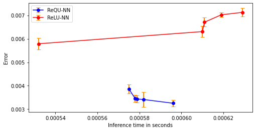
Refer to caption
Figure 4: Inference time versus error curve of ReLU and ReQU neural network.

From above, we can conclude that ReQU neural networks can achieve better accuracy with fewer inference time than ReLU neural networks when the number of layers is 5, 7, 9 and 11. However, the inference time for ReQU neural networks can be larger than that of ReLU neural networks when the number of layers equals 3, while ReQU neural networks still achieve better accuracy.

Parametric Forcing Term

We present the mean relative errors of approximating the discretized parameter to solution map by the fully connected ReQU and ReLU neural networks with the same architecture S=(4,300,…,300,4)S=(4,300,\ldots,300,4) of L=3,5,7,9,11L=3,5,7,9,11 layers, respectively.

Layers ReQU neural network ReLU neural network
3 0.000450 ±\pm 0.000020 0.000654 ±\pm 0.000041
5 0.000629 ±\pm 0.000021 0.001276 ±\pm 0.000068
7 0.000682 ±\pm 0.000123 0.001433 ±\pm 0.000078
9 0.000773 ±\pm 0.000016 0.001602 ±\pm 0.000073
11 0.000844 ±\pm 0.000051 0.001747 ±\pm 0.000142
Table 4: Test errors of the ReQU and ReLU neural networks with different numbers of layers.

The results from Table 4 show ReQU neural networks achieve smaller test errors and are more robust with respect to overfitting. In Figure 5, we depict the ground truth solution and an average performing solution predicted by the ReQU neural network with 3 layers.

Refer to caption
Figure 5: Ground truth solution and the prediction of ReQU neural network with 3 layers.

7 Discussion

In this section, we will discuss our results in terms of the dependence on the dimension of the reduced basis d⁡(ϵ~)d(\tilde{\epsilon}) and the suitability of the two assumptions 5.1 and 5.2.

7.1 Dependence on the Dimension of the Reduced Basis d⁡(ϵ~)d(\tilde{\epsilon})

To approximate parametric map

𝒴→ℝd⁡(ϵ~):y↦𝐮y,ϵ~rb\mathcal{Y}\rightarrow\mathbb{R}^{d(\tilde{\epsilon})}:\quad y\mapsto\mathbf{u}_{y,\tilde{\epsilon}}^{\mathrm{rb}}

with ϵ\epsilon accuracy, by Theorem 5.4 the number of non-zero weights of ReQU neural network required is 𝒪⁡(d3​(ϵ~)​log22⁡(log2⁡(1/ϵ))CLOSE,\mathcal{O}(d^{3}(\tilde{\epsilon})\log^{2}_{2}(\log_{2}(1/\epsilon)), while the corresponding known results is 𝒪⁡(d​(ϵ~)3​log2⁡(1/ϵ))\mathcal{O}(d(\tilde{\epsilon})^{3}\log_{2}(1/\epsilon)) for ReLU\operatorname{ReLU} network. This implies a significant advantage of ReQU over ReLU in approximating the parametric map when d⁡(ϵ~)≪log2⁡(log2⁡(1/ϵ)).d(\tilde{\epsilon})\ll\log_{2}(\log_{2}(1/\epsilon)). We remark that low rank approximations by reduced basis is achievable under certain circumstance, especially when the parametric set 𝒴\mathcal{Y} is compact. For example, the authors in [2] gave explicit low-rank representations when the diffusion coefficients are piecewise constant over a partition of the physical domain.

We illustrate this by discussing our first numerical experiment on parametric diffusion coefficients and showing that d⁡(ϵ~)d(\tilde{\epsilon}) is relatively small in this case. Recall that f⁡(𝐱)=20+10​x1−5​x2,f(\mathbf{x})=20+10x_{1}-5x_{2}, for 𝐱=(x1,x2)∈Ω=[0,1]2\mathbf{x}=(x_{1},x_{2})\in\Omega=[0,1]^{2}, which is independent of the parameters. And we parametrize the diffusion coefficient set {ay:y∈𝒴}⊂ℝp\{a_{y}:y\in\mathcal{Y}\}\subset\mathbb{R}^{p} for p=s2∈ℕp=s^{2}\in\mathbb{N} as

𝒜⁡(p,μ):={μ+∑i=1pyi​𝒳Ωi:y∈𝒴=[0,1]p},\mathcal{A}(p,\mu):=\left\{\mu+\sum_{i=1}^{p}y_{i}\mathcal{X}_{\Omega_{i}}:y\in\mathcal{Y}=[0,1]^{p}\right\},

where (Ωi)i=1p\left(\Omega_{i}\right)_{i=1}^{p} forms a s×ss\times s chessboard partition of (0,1)2(0,1)^{2}, and μ>0\mu>0 is a fixed shift. In our numerical tests, we select shifts μ=10−1\mu=10^{-1}, p=s2p=s^{2}, and s=3s=3, which yield p=9p=9. In the interior of each Ωi\Omega_{i}, we have

−(μ+∑i=1pyi​𝒳Ωi)​Δ​uy​(x)=20+10​x1−5​x2.-\left(\mu+\sum_{i=1}^{p}y_{i}\mathcal{X}_{\Omega_{i}}\right)\Delta u_{y}(x)=20+10x_{1}-5x_{2}.

Then, we can exactly solve uyu_{y} as

uy=−1μ+yi\displaystyle u_{y}=-\frac{1}{\mu+y_{i}} [\displaystyle\Bigg[ 20​(c1​x122+d1​x222)+10​(c2​x136+d2​x1​x222)+5​(c3​x122​x2+d3​x236)\displaystyle 20\left(c_{1}\frac{x_{1}^{2}}{2}+d_{1}\frac{x_{2}^{2}}{2}\right)+10\left(c_{2}\frac{x_{1}^{3}}{6}+d_{2}\frac{x_{1}x_{2}^{2}}{2}\right)+5\left(c_{3}\frac{x_{1}^{2}}{2}x_{2}+d_{3}\frac{x_{2}^{3}}{6}\right)
+c4x1x2+c5x1+c6x2+c7]\displaystyle+c_{4}x_{1}x_{2}+c_{5}x_{1}+c_{6}x_{2}+c_{7}\Bigg]

where ci+di=1c_{i}+d_{i}=1, for i∈1,2,3.i\in{1,2,3}. Thus, we obtain that

uy|Ωi∈span⁡{x12​𝒳Ωi,x22​𝒳Ωi,x13​𝒳Ωi,x1​x22​𝒳Ωi,x12​x2​𝒳Ωi,x23​𝒳Ωi,x1​x2​𝒳Ωi,x1​𝒳Ωi,x2​𝒳Ωi,𝒳Ωi}.\left.u_{y}\right|_{\Omega_{i}}\in\operatorname{span}\left\{x_{1}^{2}\mathcal{X}_{\Omega_{i}},x_{2}^{2}\mathcal{X}_{\Omega_{i}},x_{1}^{3}\mathcal{X}_{\Omega_{i}},x_{1}x_{2}^{2}\mathcal{X}_{\Omega_{i}},x_{1}^{2}x_{2}\mathcal{X}_{\Omega_{i}},x_{2}^{3}\mathcal{X}_{\Omega_{i}},x_{1}x_{2}\mathcal{X}_{\Omega_{i}},x_{1}\mathcal{X}_{\Omega_{i}},x_{2}\mathcal{X}_{\Omega_{i}},\mathcal{X}_{\Omega_{i}}\right\}.

This yields an upper bound of 10×9=9010\times 9=90 degrees of freedom for uyu_{y}. Since there are 2424 continuity conditions (independent of yy ) on uu at domain and subinterval boundaries, we have

rank⁡(u)≤90−24=66\operatorname{rank}(u)\leq 90-24=66

and therefore d⁡(ϵ~)≤66d(\tilde{\epsilon})\leq 66, independent of the particular choice of ϵ~\tilde{\epsilon}.

7.2 Suitability of Assumptions 5.1 and 5.2

Indeed, the two assumptions 5.1 and 5.2 hold if the maps y↦by​(u,v)y\mapsto b_{y}(u,v) and y→fy​(v)y\rightarrow f_{y}(v) are continuous for all u,v∈ℋu,v\in\mathcal{H}. In this case, it is enough to show that ReQU neural networks can approximate continuous function. By [17, Theorem3.1], ReQU neural network can represent multivariate polynomial on ℝd\mathbb{R}^{d} with no error. Thus, by the Weierstrass approximation theorem, assumption 5.1 and 5.2 can be achieved.

Next, we discuss about the required size for the ReQU-realizations of the maps y↦𝐁y,ϵ~rby\mapsto\mathbf{B}_{y,\tilde{\epsilon}}^{\mathrm{rb}} and y↦𝐟y,ϵ~rby\mapsto\mathbf{f}_{y,\tilde{\epsilon}}^{\mathrm{rb}}, taking our first numerical experiment for example again. We write the parametric diffusion equation

−∇⋅(ay(𝐱)⋅∇uy(𝐱))=f(𝐱), on Ω=(0,1)2,uy|∂Ω=0-\nabla\cdot\left(a_{y}(\mathbf{x})\cdot\nabla u_{y}(\mathbf{x})\right)=f(\mathbf{x}),\quad\text{ on }\Omega=(0,1)^{2},\left.\quad u_{y}\right|_{\partial\Omega}=0

in its variation form

By(uy,v):=∫Ωμ∇uy∇vd𝐱+∑i=1pyi∫Ω𝒳Ωi∇uy∇vd𝐱=f(v), for all v∈ℋ.B_{y}\left(u_{y},v\right):=\int_{\Omega}\mu\nabla u_{y}\nabla v\mathrm{~d}\mathbf{x}+\sum_{i=1}^{p}y_{i}\int_{\Omega}\mathcal{X}_{\Omega_{i}}\nabla u_{y}\nabla v\mathrm{~d}\mathbf{x}=f(v),\quad\text{ for all }v\in\mathcal{H}.

By the definition of 𝐁y,ϵ~rb:=(By​(ψj,ψi))i,j=1d⁡(ϵ~)\mathbf{B}_{y,\tilde{\epsilon}}^{\mathrm{rb}}:=\left(B_{y}\left(\psi_{j},\psi_{i}\right)\right)_{i,j=1}^{d(\tilde{\epsilon})} and Lemma 2.2, we can derive

yi=β1T​σ2​(ω1​yi+γ1),y_{i}=\mathbf{\beta}_{1}^{T}\sigma_{2}\left(\mathbf{\omega}_{1}y_{i}+\mathbf{\gamma}_{1}\right),

where ω1=[1,−1,1,−1]T,γ1=[1,−1,−1,1]T\mathbf{\omega}_{1}=[1,-1,1,-1]^{T},\mathbf{\gamma}_{1}=[1,-1,-1,1]^{T} and β1=14​[1,1,−1,−1]T\mathbf{\beta}_{1}=\frac{1}{4}[1,1,-1,-1]^{T}. Thus, we have for ϵ~,ϵ>0\tilde{\epsilon},\epsilon>0,

BL​(ϵ~,ϵ)=2,\displaystyle B_{L}(\tilde{\epsilon},\epsilon)=2,
FL​(ϵ~,ϵ)=1,\displaystyle F_{L}(\tilde{\epsilon},\epsilon)=1,
BM​(ϵ~,ϵ)≤(‖ω1‖0+‖γ1‖0)​p+(4​p+1)​d​(ε~)2=8​p+(4​p+1)​d​(ε~)2,\displaystyle B_{M}(\tilde{\epsilon},\epsilon)\leq\left(\left\|\omega_{1}\right\|_{0}+\left\|\gamma_{1}\right\|_{0}\right)p+(4p+1)d(\tilde{\varepsilon})^{2}=8p+(4p+1)d(\tilde{\varepsilon})^{2},
FM​(ϵ~,ϵ)≤p​d​(ϵ~).\displaystyle F_{M}(\tilde{\epsilon},\epsilon)\leq pd(\tilde{\epsilon}).

Combining this observation with the statement of Theorem 5.4, we can conclude that the governing quantity in the obtained number of layers and complexity bound are given by 𝒪⁡(log22⁡(log2⁡(1/ϵ))CLOSE\mathcal{O}(\log^{2}_{2}(\log_{2}(1/\epsilon)) and 𝒪⁡(d3​(ϵ~)​log22⁡(log2⁡(1/ϵ))CLOSE\mathcal{O}(d^{3}(\tilde{\epsilon})\log^{2}_{2}(\log_{2}(1/\epsilon)) respecitively.

8 Conclusion

In this paper, we give constructive proofs of complexity bounds for approximating parametric map by deep neural networks using ReQU function as the activation functions. In contrast to the previously established complexity-bound 𝒪⁡(d3​log2q⁡(1/ϵ))\mathcal{O}\left(d^{3}\log_{2}^{q}(1/\epsilon)\right) for ReLU neural networks, we derive an upper bound 𝒪⁡(d3​log2q​log2⁡(1/ϵ))\mathcal{O}\left(d^{3}\log_{2}^{q}\log_{2}(1/\epsilon)\right) on the size of the deep ReQU neural network required to achieve accuracy ϵ>0\epsilon>0. This implies the better performance of deep ReQU neural networks in solving parametric partial differential equations. In addition, we compare the practical performance of deep neural networks approximation based on ReLU versus ReQU on two parametric PDE models. These numerical experiments indicate that ReQU neural networks can achieve smaller errors than ReLU neural networks, at identical network architecture hyperparameters (depth and layer widths). Furthermore, ReQU neural networks converge more quickly in the optimization and are more stable with respect to overfitting.

This work opens up many interesting directions for future research. First of all, for both ReLU and ReQU based methods, the reduced basis approximation for model reduction on function spaces could be improved by adaptive data-driven approaches such as the kernel proper orthogonal decomposition (KPOD) and principal component analysis (PCA) techniques, see [3, 25]. Furthermore, a limitation of this study is that our findings indicate ReQU neural networks with sufficient layers and size can provide accurate approximations, but we do not know how to choose the ideal neural network architectures for the specific problem in applications. As a future work, we plan to conduct a comprehensive experiment to investigate the theoretical setup of this paper, including using other special architectures like convolutional neural networks and generalizing to more general parametric problems. Finally, we also want to apply our methodology to more difficult PDE problems, such as complex PDE models in the sciences and in engineering and numerical solution of forward and inverse problems of parametric and stochastic PDEs.

Acknowledgement

We would like to thank the two anonymous reviewers for their helpful and constructive comments on our work.

Funding

The authors were in part supported by NSFC (Grant No. 11725102), National Support Program for Young Top-Notch Talents, and Shanghai Science and Technology Program (Project No. 21JC1400600, No. 19JC1420101, and No. 20JC1412700).

Data Availability

The dataset is available at www.github.com/MoGeist/diffusion_PPDE.

Declarations

Competing interests

The authors have not disclosed any competing interests.

References

  • [1] Martin Alnæs, Jan Blechta, Johan Hake, August Johansson, Benjamin Kehlet, Anders Logg, Chris Richardson, Johannes Ring, Marie E Rognes, and Garth N Wells. The fenics project version 1.5. Archive of Numerical Software, 3(100), 2015.
  • [2] Markus Bachmayr and Albert Cohen. Kolmogorov widths and low-rank approximations of parametric elliptic pdes. Mathematics of Computation, 86(304):701–724, 2017.
  • [3] Kaushik Bhattacharya, Bamdad Hosseini, Nikola B Kovachki, and Andrew M Stuart. Model reduction and neural networks for parametric pdes. SMAI J. Comput. Math., 7:121–157, 2021.
  • [4] Charles K Chui and Hrushikesh N Mhaskar. Deep nets for local manifold learning. Front. Appl. Math. Stat., 4:12, 2018.
  • [5] Niccolò Dal Santo, Simone Deparis, and Luca Pegolotti. Data driven approximation of parametrized pdes by reduced basis and neural networks. J. Comput. Phys., 416:109550, 2020.
  • [6] Chenguang Duan, Yuling Jiao, Yanming Lai, Dingwei Li, Jerry Zhijian Yang, et al. Convergence rate analysis for deep ritz method. Communications in Computational Physics, 31(4):1020–1048, 2022.
  • [7] Dennis Elbrachter, Philipp Grohs, Arnulf Jentzen, and Christoph Schwab. Dnn expression rate analysis of high-dimensional pdes: Application to option pricing. Constr. Approx., 2018.
  • [8] Lawrence C. Evans. Partial differential equations, volume 19 of Graduate Studies in Mathematics. American Mathematical Society, Providence, RI, second edition, 2010.
  • [9] Moritz Geist, Philipp Petersen, Mones Raslan, Reinhold Schneider, and Gitta Kutyniok. Numerical solution of the parametric diffusion equation by deep neural networks. Journal of Scientific Computing, 88(1):1–37, 2021.
  • [10] Jiequn Han, Arnulf Jentzen, and E Weinan. Solving high-dimensional partial differential equations using deep learning. Proc. Nat. Acad. Sci., 115(34):8505–8510, 2018.
  • [11] Juncai He, Lin Li, Jinchao Xu, and Chunyue Zheng. Relu deep neural networks and linear finite elements. J. Comput. Math., 38(3):502, 2020.
  • [12] Jan S Hesthaven, Gianluigi Rozza, Benjamin Stamm, et al. Certified reduced basis methods for parametrized partial differential equations, volume 590. Springer, 2016.
  • [13] Yuehaw Khoo, Jianfeng Lu, and Lexing Ying. Solving parametric pde problems with artificial neural networks. European J. Appl. Math., 32(3):421–435, 2021.
  • [14] Nikola Kovachki, Samuel Lanthaler, and Siddhartha Mishra. On universal approximation and error bounds for fourier neural operators. J. Mach. Learn. Res., 22:Art–No, 2021.
  • [15] Gitta Kutyniok, Philipp Petersen, Mones Raslan, and Reinhold Schneider. A theoretical analysis of deep neural networks and parametric pdes. Constr. Approx., pages 1–53, 2021.
  • [16] Samuel Lanthaler, Siddhartha Mishra, and George Karniadakis. Error estimates for deeponets: A deep learning framework in infinite dimensions. SAM Research Report, 2021, 2021.
  • [17] Bo Li, Shanshan Tang, and Haijun Yu. Better approximations of high dimensional smooth functions by deep neural networks with rectified power units. Commun. Comput. Phys., 27:379–411, 2020.
  • [18] Zongyi Li, Nikola Borislavov Kovachki, Kamyar Azizzadenesheli, Kaushik Bhattacharya, Andrew Stuart, Anima Anandkumar, et al. Fourier neural operator for parametric partial differential equations. In International Conference on Learning Representations, 2020.
  • [19] Lu Lu, Pengzhan Jin, and George Em Karniadakis. Deeponet: Learning nonlinear operators for identifying differential equations based on the universal approximation theorem of operators. arXiv preprint arXiv:1910.03193, 2019.
  • [20] Hrushikesh N Mhaskar. Neural networks for optimal approximation of smooth and analytic functions. Neural Comput., 8(1):164–177, 1996.
  • [21] Hrushikesh Narhar Mhaskar. Approximation properties of a multilayered feedforward artificial neural network. Adv. Comput. Math., 1(1):61–80, 1993.
  • [22] Joost AA Opschoor, Ch Schwab, and Jakob Zech. Exponential relu dnn expression of holomorphic maps in high dimension. Constr. Approx., pages 1–46, 2021.
  • [23] Adam Paszke, Sam Gross, Francisco Massa, Adam Lerer, James Bradbury, Gregory Chanan, Trevor Killeen, Zeming Lin, Natalia Gimelshein, Luca Antiga, et al. Pytorch: An imperative style, high-performance deep learning library. Advances in neural information processing systems, 32:8026–8037, 2019.
  • [24] Alfio Quarteroni, Andrea Manzoni, and Federico Negri. Reduced basis methods for partial differential equations: an introduction, volume 92. Springer, 2015.
  • [25] Matteo Salvador, Luca Dede, and Andrea Manzoni. Non intrusive reduced order modeling of parametrized pdes by kernel pod and neural networks. Computers &\& Mathematics with Applications, 104:1–13, 2021.
  • [26] Christoph Schwab and Jakob Zech. Deep learning in high dimension: Neural network expression rates for generalized polynomial chaos expansions in uq. Anal. Appl. (Singap.), 17(01):19–55, 2019.
  • [27] Justin Sirignano and Konstantinos Spiliopoulos. Dgm: A deep learning algorithm for solving partial differential equations. J. Comput. Phys., 375:1339–1364, 2018.
  • [28] Shanshan Tang, Bo Li, and Haijun Yu. Chebnet: Efficient and stable constructions of deep neural networks with rectified power units using chebyshev approximations. arXiv preprint arXiv:1911.05467, 2019.
  • [29] Dmitry Yarotsky. Error bounds for approximations with deep relu networks. Neural Netw., 94:103–114, 2017.