跳到论文正文
W Papers独立论文阅读器 arXiv:2203.06837 论文正文 计算阅读时间 · 0%
引用这篇论文根据当前论文元数据生成,正式投稿前建议核对。


License: arXiv.org perpetual non-exclusive license
arXiv:2203.06837v2 [econ.TH] 06 Sep 2022

Beckmann’s approach to multi-item multi-bidder auctionsWe are grateful to Federico Echenique, Luciano Pomatto, Joseph Root, and Omer Tamuz for conversations that inspired this work. We also thank Luciano for multiple suggestions improving the manuscript. The paper benefited from discussions with Kim Border, Benjamin Brooks, Alkis Georgiadis-Harris, Sergiu Hart, Jason Hartline, Andreas Kleiner, Alexey Kushnir, Alejandro Manelli, Robert McCann, Benny Moldovanu, and Philip J. Reny and from comments by seminar participants at the University of Bonn, INFORMS Workshop on Market Design 2022, the 33rd Stony Brook Game Theory Conference, and Yale University. Thanks: Sandomirskiy thanks Linde Institute at Caltech and National Science Foundation (grant CNS 1518941).

Alexander V. Kolesnikov (HSE University) Thanks: Kolesnikov acknowledges the support of RSF Grant №22-21-00566 https://rscf.ru/en/project/22-21-00566/. The article was prepared within the framework of the HSE University Basic Research Program. Affiliation: Fedor Sandomirskiy (Caltech) Affiliation: Aleh Tsyvinski (Yale) Affiliation: Alexander P. Zimin (MIT and HSE University)
Abstract

We consider the problem of revenue-maximizing Bayesian auction design with several bidders having independent private values over several items. We show that it can be reduced to the problem of continuous optimal transportation introduced by Beckmann 1952 where the optimal transportation flow generalizes the concept of ironed virtual valuations to the multi-item setting. We establish the strong duality between the two problems and the existence of solutions. The results rely on insights from majorization and optimal transportation theories and on the characterization of feasible interim mechanisms by Hart and Reny 2015.

1 Introduction

The current understanding of multi-bidder multi-item revenue-maximizing auctions is far from being complete even in the basic setting of several bidders competing for several items and having i.i.d. additive utilities over them. Only the case of one item and several bidders was analyzed completely (Myerson 1981). A seemingly innocent problem with one bidder and several items already turns out to be notoriously difficult to analyze, optimal mechanisms are known only in a few particular cases and exhibit complicated structure (Armstrong and Rochet 1999, Rochet and Stole 2003, Daskalakis 2015). If both the number of bidders and the number items exceed one, we get a benchmark problem combining the difficulty of mechanism design with multi-dimensional types and that with multiple agents. Essentially, nothing has been known about optimal auctions in this setting.

The main contribution of our paper is to establish an unexpected connection between the problem of auction design and an optimal transportation problem in the classic model of Beckmann 1952. In contrast to the prevalent Monge-Kantorovich approach, Beckmann’s paradigm of “continuous transportation” captures the trajectories along which transportation occurs.

Imagine a commodity that is produced and consumed at different geographic locations and so the product has to be transported. Theory of optimal transportation aims to find the least costly way of doing that for given spacial distributions of production and consumption and given transportation costs. Beckmann 1952 modelled the process of transportation as a continuous flow. Its intensity and direction at each point defines a vector and the problem is to find the vector field with minimal cost. More formally, let πp​(x)\pi_{p}(x) and πc​(x)\pi_{c}(x) be the density of production and consumption at a given point xx in some Euclidean space and ρ=ρ⁡(x)\rho=\rho(x) be a weight function. Let c=c⁡(x)c=c(x) be a vector field representing the direction and the intensity of the flow. The flow is chosen to compensate supply-demand imbalances, i.e., the difference between the weighted inflow and outflow in a region has to be equal to the difference between supply and demand in it. This compensation boils down to the condition that the divergence div⁡[ρ⋅c]{\mathrm{div}}[\rho\cdot c] (the sum of partial derivatives) must be equal to πp−πc\pi_{p}-\pi_{c}. Let Φ⁡(c⁡(x))\Phi(c(x)) be the local cost of transportation. For given πp,πc\pi_{p},\pi_{c}, ρ\rho, and Φ\Phi, Beckmann’s problem is to find the flow cc compensating imbalances and having the minimal total cost:

minc:div⁡[ρ⋅c]+πc−πp=0∫Φ(c(x))ρ(x)dx.\min_{c:\ {\mathrm{div}}[\rho\cdot c]+\pi_{c}-\pi_{p}=0}\int\Phi\left(c(x)\right)\rho(x){\,\mathrm{d}}x. (1)

We demonstrate that a dual problem to revenue maximization takes the form of Beckmann’s problem (1) with a particular cost function Φ\Phi and marginals πp\pi_{p} and πc\pi_{c} satisfying a certain majorization constraint. Locations xx represent bidders’ types and the field cc corresponds to ironed virtual valuations. Similar generalizations of Beckmann’s problem are related to mean-field limits of the Wardrop equilibria for congested optimal transportation games (Santambrogio 2015, Carlier 2012) but have not appeared in the context of auction design.

We establish the strong duality, namely, the optimal revenue of the auctioneer equals the optimal value of the dual problem. The strong duality is especially useful if combined with the existence of solutions — i.e., if the optima are attained — as this combination enables complementary slackness conditions. We demonstrate both the existence of an optimal auction and an optimal vector field cc, which are one of the most technically challenging parts of the paper.

Applications and simulations.

We illustrate a use of duality by recovering the result of Jehiel et al. 2007 that selling several items with independent values separately is never optimal provided that values are continuously distributed. This amounts to checking that complementary slackness conditions become incompatible whenever the allocation of each item depends on the values for this item only.

Complementary slackness suggests a guess-and-verify approach: first one guesses a solution to the primal problem, uses complementary slackness to find a dual solution, and this dual solution plays a role of a certificate verifying the initial guess. We illustrate this approach in the cases of one item and multiple bidders or one bidder and two items with i.i.d. uniform values where the optimal mechanism was found by Manelli and Vincent 2006; see Appendix D.

A prerequisite for the guess-and-verify approach is the existence of a simple explicit solution. To get insights into the structure of optimal auctions, we compute them numerically for several bidders having uniformly distributed values over two items. These simulations indicate the complexity of the optimal mechanism even in this benchmark setting. In particular, the optimal auction does not seem to be given by an elementary function.11 1 Proposing candidates for an optimal auction format remains a major open problem in the multi-item multi-bidder setting. Note that selling separately or selling the grand bundle are never optimal (Jehiel et al. 2007). We bound the revenue loss from using sub-optimal designs and show how the conclusions change as the number of bidders grows.

To compute the optimal auctions, we develop a new numerical approximation scheme that allows one to conduct simulations that were previously out of reach.22 2 Even the advanced neural-network approach of (Dütting et al. 2019) does not produce the outcome detailed and reliable enough to make structural conclusions because of the curse of dimensionality. The approach relies on a combination of multi-to-single-agent reduction of Cai et al. 2012 and Alaei et al. 2019 avoiding the curse of dimensionality at the cost of dealing with a non-linear feasibility constraint, majorization theory insights (Kleiner et al. 2021) to linearize this constraint, duality to Beckmann’s problem to guarantee that a solution of a discretized problem is close to that of the continuous one, and cutting-edge numerical methods to handle optimization over convex functions speeding up the algorithm in practice. As far as we know, algorithms based on multi-to-single-agent reduction have never been previously implemented.

Single bidder versus multiple bidders.

To get more intuition about our approach and to highlight the specific features of the multi-bidder setting, we compare it to the single-bidder benchmark of the monopolist’s problem.

An important advance in understanding the monopolist’s problem was made by Daskalakis et al. 2017 who showed how to reduce it to an optimal transportation one. Instead of Beckmann’s problem arising in the multi-bidder setting, the dual derived by Daskalakis et al. 2017 is the Monge–Kantorovich optimal transportation problem with a majorization constraint. The Monge–Kantorovich problem has the following form:

minγ:γ1=πp,γ2=πc∫|x−y|dγ(x,y),\min_{\gamma:\ \gamma_{1}=\pi_{p},\ \gamma_{2}=\pi_{c}}\int|x-y|{\,\mathrm{d}}\gamma(x,y), (2)

where πp​(x)​d​x\pi_{p}(x){\,\mathrm{d}}x is the geographical distribution of production, πc​(y)​d​y\pi_{c}(y){\,\mathrm{d}}y is the distribution of consumption, and the goal is to find a transportation plan γ\gamma such that the total transportation cost given by the integral in (2) is minimal and supply meets demand, i.e., the marginal of γ\gamma on the first coordinate is πp\pi_{p} and on the second, πc\pi_{c}. In contrast to Beckmann’s problem, the transportation happens momentarily: only initial and final destinations are captured by the plan γ\gamma, not the trajectories connecting them.

We conclude that the revenue-maximization problem for a single-bidder has two differently looking optimal-transportation duals: the Monge–Kantorovich dual and Beckmann’s one. This indicates the connection between the two duals themselves, in particular, their values must be equal. It turns out that for a single bidder, the cost function Φ\Phi in Beckmann’s problem can be simplified to Φ⁡(x)=|x|\Phi(x)=|x|. For this cost function, the values of (1) and (2) are known to coincide by the so-called Beckmann’s duality (Santambrogio 2015, Section 4.2). The presence of the two duals for the monopolist’s problem is a repercussion of this duality.

For a single bidder, one can use any of the two duals. However, the link between revenue maximization and the Monge–Kantorovich problem turns out to be limited to the single-bidder case. By contrast, the connection to Beckmann’s problem generalizes to any number of bidders and items.

Let us highlight the key features of the approach allowing us to handle the multi-bidder case. The standard first step in the analysis of the monopolist’s problem is replacing the non-tractable maximization over mechanism via a handy maximization over interim utility functions u=u⁡(x)u=u(x), where xx is the buyer’s type (Rochet and Choné 1998). The Rochet-Choné representation is the starting point for the analysis of Daskalakis et al. 2017. The corresponding optimization problem is of the form

max⁡∫u⁡(⟨∇u​(x),x⟩−u⁡(x))​ρ​(x)​𝑑x,\max_{u}\int\Big(\langle\nabla u(x),x\rangle-u(x)\Big)\rho(x){\,\mathrm{d}}x,

where the maximum is taken over non-decreasing convex non-negative 11-Lipschitz functions uu.

The Rochet-Choné representation can be generalized to multi-bidder problems at the cost of getting an extra constraint capturing feasibility of the corresponding interim allocation rule. Most of the literature relies on a form of this constraint conjectured by Matthews 1984 and proved by Border 1991.

The key role in our approach is played by a less known form of this feasibility condition discovered by Hart and Reny 2015 and extended to the multi-item setting in our paper. The condition takes a form of a majorization constraint on the distribution of uu’s gradient. The connection to majorization theory fuels our analysis and simulations. This theory has multiple recent applications in economic design; see, e.g., (Kleiner et al. 2021, Arieli et al. 2019, Candogan and Strack 2021, Nikzad 2022, Gershkov et al. 2021).

The non-local majorization constraint determines the crucial difference between the resulting multi-bidder Rochet-Choné representation and its single-bidder version. It does not allow us to get rid of the derivatives of uu, which was crucial for the approach of Daskalakis et al. 2017. This obstacle explains why their approach does not generalize to the multi-bidder setting and why our dual problem does not look similar to the Monge-Kantorovich one. The non-local constraint is a major complication; it leads to involved functional classes needed to establish strong duality and the existence of a solution to the dual. We note that demonstrating strong duality with non-local constraints is new not just for the economic literature but also to the broader mathematical context.

Related literature

Linear programs and their duals are ubiquitous in microeconomics and economic design (Vohra 2011, Bichler 2017). The modern literature is increasingly interested in infinite-dimensional settings (corresponding to non-atomic type spaces) as they highlight geometric properties of solutions such as differentiability, convexity, and links to majorization. Apart from multi-item auctions discussed below, infinite-dimensional linear programs and their duals naturally arise in various contexts, e.g., informationally or distributionally robust auction design (Bergemann et al. 2016, Koçyiğit et al. 2020, Suzdaltsev 2020), information economics (Kolotilin 2018, Dworczak and Martini 2019, Dizdar and Kováč 2020, Arieli et al. 2021a). Infinite-dimensional programs often have the structure similar to the Monge-Kantorovich optimal transportation, for example, in the context of sorting on the labor market (Boerma et al. 2021), matching with transferable utility and principal-agent problems (Chiappori et al. 2010), econometrics (Galichon 2021), optimal taxation (Steinerberger and Tsyvinski 2019), strategic learning and forecasting (Gensbittel 2015, Arieli et al. 2021b, Guo and Shmaya 2021). Other economic applications of optimal transport can be found in (Figalli et al. 2011, McCann and Zhang 2019) and are surveyed by Galichon 2016 and Carlier 2012. For non-linear economic problems, a dual approach sharing some similarity with optimal transportation duality was proposed by Nöldeke and Samuelson 2018. A comprehensive presentation of the mathematical theory of transportation can be found in the books by Santambrogio 2015 and Villani 2009 and in surveys Bogachev and Kolesnikov 2012, Guillen and McCann 2013.

The continuous model of transportation developed by Beckmann 1952 is one of the classical economic models of transport networks that had considerable early popularity. It has not been used much in the recent economic literature with the exception of spatial equilibrium models of Fajgelbaum and Schaal 2020 and Allen and Arkolakis 2014. Beckmann’s problem has anticipated the dynamic perspective on optimal transportation playing an important role in the modern theory; see the discussion in in Appendix F. This perspective is central for cutting-edge machine learning techniques such as the Wasserstein gradient flows (Peyré and Cuturi 2019, Kolouri et al. 2017). Beckmann’s problem depends on the difference between production and consumption distributions but not on the distributions per se which makes it similar to the transshipment problem, a version of the Monge-Kantorovich problem where the distributions are not fixed but their difference is (Rachev and Rüschendorf 2006). Beckmann’s problem can be seen as a dynamic version of the transshipment problem (Carlier and Santambrogio 2005).

For infinite-dimensional problems, the central questions become whether the duality gap is zero or not (strong versus weak duality) and whether primal and dual solutions exist. Both strong duality and the existence are needed for complementary slackness conditions to hold. In auction design, these questions have only been studied in the single-bidder case. Daskalakis et al. 2017 established the connection to optimal transport, demonstrated the strong duality, and showed the existence; their proofs were then simplified by Kleiner and Manelli 2019. For several bidders, Giannakopoulos and Koutsoupias 2018 partially relaxed the incentive-compatibility constraint and got a weakly dual problem sharing some similarity with the maximal flow one. In contrast to our paper, they did not discuss the issue of existence as non-zero duality gap diminishes the importance of this question. Cai et al. 2019 considered a general problem of Bayesian mechanism design with finite number of types and derived a strongly dual problem resembling the maximal flow one. As the problem is finite-dimensional, the existence questions become mute and the strong duality is a consequence of the standard linear programming duality. A similar duality approach was outlined by Myerson 2002 who, however, focused on bargaining applications and did not discuss auctions. None of these papers relied on multi-to-single-agent reduction; this simplified the derivation of the duals at the cost of getting high-dimensional problems for B≥2B\geq 2 agents.

Even for a single bidder, optimal multi-item auctions can be complex and require non-linear pricing of a continuum of fractional bundles; explicit answers are known in a few particular cases such as uniformly or exponentially distributed values (Daskalakis et al. 2017). A primal approach of Haghpanah and Hartline 2021 based on virtual surplus maximization provides an alternative to optimal transportation technique of Daskalakis et al. 2017 and, in some cases, pins down an optimal mechanism, e.g., it shows when pure bundling is optimal in the single-bidder case; see also (Hartline 2013, Chapter 8). Instead of looking for optimal mechanisms the literature has mainly focused on either showing that a simple mechanism can guarantee a certain fraction of the optimal revenue or asking how well one can approximate the optimal mechanism withing a certain parametric class; see representative papers (Hart and Reny 2019, Babaioff et al. 2020) and (Hart and Nisan 2017, Babaioff et al. 2021). The only explicitly solved multi-item auction with several bidders assumes that bidders’ valuations are binary (Yao 2017).

2 Model

We work in the standard setting of Bayesian auction design with quasilinear bidders having i.i.d. additive utilities over items.

There is a set ℬ={1,2,…,B}\mathcal{B}=\{1,2,\ldots,B\} of B≥1B\geq 1 bidders and a set ℐ={1,2,…,I}\mathcal{I}=\{1,2,\ldots,I\} of I≥1I\geq 1 items. We assume that the items are divisible and normalize the total amount of each item to one unit. As usual, indivisible items can be made divisible by interpreting fractional amounts as probability shares.

Bidders treat the items as perfect substitutes and, hence, bidders’ preferences are modelled by additive utility functions quasi-linear in money. The utility function of a bidder b∈ℬb\in\mathcal{B} receiving a bundle pb∈ℝ+ℐp_{b}\in\mathbb{R}_{+}^{\mathcal{I}} of items for a price tbt_{b} takes the form

⟨pb,xb⟩−tb,\left\langle p_{b},x_{b}\right\rangle-t_{b},

where ⟨⋅,⋅⟩\left\langle\cdot,\cdot\right\rangle is the standard dot product in ℝℐ\mathbb{R}^{\mathcal{I}} and the vector xb∈ℝ+ℐx_{b}\in\mathbb{R}_{+}^{\mathcal{I}} specifies bb’s maximal willingness to pay for each of the items. The vector xbx_{b} can be seen as bidder bb’s type and constitutes the bidder’s private information. Each bidder’s type xbx_{b} belongs to the set of types33 3 This assumption is without loss of generality as any bounded set of types can be made a subset of [0,1]ℐ[0,1]^{\mathcal{I}} by rescaling. X=[0,1]ℐX=[0,1]^{\mathcal{I}}.

We assume that the fraction of bidders of different types in the population is described by a density ρ\rho positive on XX and zero beyond. The bidders are chosen from this population independently and, hence, the types xb∈Xx_{b}\in X, b∈ℬb\in\mathcal{B}, are i.i.d. draws with the distribution μ\mu where d​μ​(xb)=ρ⁡(xb)​d​xb{\,\mathrm{d}}\mu(x_{b})=\rho(x_{b}){\,\mathrm{d}}x_{b}. The auctioneer and bidders know ρ\rho and each bidder observes the realization of her own type.

A mechanism which we also refer to as auction is given by a collection of bundles P=(Pb​(x))b∈ℬP=(P_{b}(x))_{b\in\mathcal{B}} and transfers T=(Tb​(x))b∈ℬT=(T_{b}(x))_{b\in\mathcal{B}} for each profile of types x=(xb)b∈ℬx=(x_{b})_{b\in\mathcal{B}}. Formally, a mechanism (P,T)(P,T) is a measurable map Xℬ→ℝ+ℐ×ℬ×ℝℬX^{\mathcal{B}}\to\mathbb{R}_{+}^{\mathcal{I}\times\mathcal{B}}\times\mathbb{R}^{\mathcal{B}}:

(xb)b∈ℬ→(Pb​((xb)b∈ℬ),Tb​((xb)b∈ℬ))b∈ℬ.(x_{b})_{b\in\mathcal{B}}\ \to\ \Big(P_{b}\big((x_{b})_{b\in\mathcal{B}}\big),\ T_{b}\big((x_{b})_{b\in\mathcal{B}}\big)\Big)_{b\in\mathcal{B}}.

Here PbP_{b} is the bundle received by a bidder b∈ℬb\in\mathcal{B} and TbT_{b} is the amount of money she pays to the auctioneer. A mechanism is feasible if for any profile of types (xb)b∈ℬ(x_{b})_{b\in\mathcal{B}}

∑b∈ℬPb,i​((xb)b∈ℬ)≤1for all items i∈ℐ,\sum_{b\in\mathcal{B}}P_{b,i}\big((x_{b})_{b\in\mathcal{B}}\big)\leq 1\quad\mbox{for all items $i\in\mathcal{I}$,} (3)

i.e., the auctioneer has only one unit of each item to sell and so a mechanism cannot allocate more than one unit.

The auctioneer aims to design an auction maximizing the expected revenue ∑b∈ℬTb\sum_{b\in\mathcal{B}}T_{b}. Bidders’ types are their private information and a bidder may misreport her type if this brings her higher utility. Similarly, participation is voluntary and bidders may decide not to take part in the auction if they do not expect this to be profitable. Hence, providing incentives for truthful behavior and participation becomes design constraints. To formalize them, compute the expected allocation and transfer faced by a bidder bb of a given type xbx_{b} assuming that others report their types truthfully:

P¯b​(xb)\displaystyle\overline{P}_{b}(x_{b}) =∫Xℬ∖{b}Pb((xb)b∈ℬ)⋅(∏d∈ℬ∖{b}ρ(xd))dx1⋯dxb−1dxb+1⋯dxB,\displaystyle=\int_{X^{{\mathcal{B}}\setminus\{b\}}}P_{b}\big((x_{b})_{b\in\mathcal{B}}\big)\cdot\left(\prod_{d\in{\mathcal{B}}\setminus\{b\}}\rho(x_{d})\right){\,\mathrm{d}}x_{1}\cdots{\,\mathrm{d}}x_{b-1}{\,\mathrm{d}}x_{b+1}\cdots{\,\mathrm{d}}x_{B}, (4)
T¯b​(xb)\displaystyle\overline{T}_{b}(x_{b}) =∫Xℬ∖{b}Tb((xb)b∈ℬ)⋅(∏d∈ℬ∖{b}ρ(xd))dx1⋯dxb−1dxb+1⋯dxB.\displaystyle=\int_{X^{{\mathcal{B}}\setminus\{b\}}}T_{b}\big((x_{b})_{b\in\mathcal{B}}\big)\cdot\left(\prod_{d\in{\mathcal{B}}\setminus\{b\}}\rho(x_{d})\right){\,\mathrm{d}}x_{1}\cdots{\,\mathrm{d}}x_{b-1}{\,\mathrm{d}}x_{b+1}\cdots{{\,\mathrm{d}}}x_{B}. (5)

Such one-bidder marginals (P¯b,T¯b)(\overline{P}_{b},\overline{T}_{b}) of the original mechanism (P,T)(P,T) are known as its reduced forms or interim mechanisms. The reduced mechanism for a bidder bb captures how her expected utility depends on her type and her report, i.e., all the information relevant to her: if her type is xbx_{b} and she reports to be of type xb′x_{b}^{\prime}, while other bidders remain truthful, bb’s expected utility takes the form

⟨P¯b​(xb′),xb⟩−T¯b​(xb′).\big\langle\overline{P}_{b}(x_{b}^{\prime}),\,x_{b}\big\rangle-\overline{T}_{b}(x_{b}^{\prime}).

A mechanism is called Bayesian incentive-compatible if truth-telling is a Bayesian equilibrium, i.e., no bidder bb has an incentive to misreport her values if others report truthfully. Formally,

⟨P¯b​(xb),xb⟩−T¯b​(xb)≥⟨P¯b​(xb′),xb⟩−T¯b​(xb′)\big\langle\overline{P}_{b}(x_{b}),\,x_{b}\big\rangle-\overline{T}_{b}(x_{b})\geq\langle\overline{P}_{b}(x_{b}^{\prime}),\,x_{b}\rangle-\overline{T}_{b}(x_{b}^{\prime}) (6)

for all xb,xb′∈Xx_{b},x_{b}^{\prime}\in X and b∈ℬ.b\in\mathcal{B}.

A mechanism is called individually rational if no bidder wants to abstain from participation, i.e., nobody gets a negative expected utility. Formally,

⟨P¯b​(xb),xb⟩−T¯b​(xb)≥0\big\langle\overline{P}_{b}(x_{b}),\,x_{b}\big\rangle-\overline{T}_{b}(x_{b})\geq 0 (7)

for all xb∈Xx_{b}\in X and b∈ℬ.b\in\mathcal{B}.

The auctioneer’s design problem takes the following form.

Auctioneer’s problem: maximize the expected revenue

∫Xℬ(∑b∈ℬTb((xb)b∈ℬ))⋅(∏b∈ℬρ(xb))dx1⋯dxB\int_{X^{\mathcal{B}}}\left(\sum_{b\in\mathcal{B}}T_{b}\big((x_{b})_{b\in\mathcal{B}}\big)\right)\cdot\left(\prod_{b\in\mathcal{B}}\rho(x_{b})\right){\,\mathrm{d}}x_{1}\cdots{\,\mathrm{d}}x_{B} (8)

over individually-rational Bayesian incentive-compatible feasible mechanisms (P,T)(P,T).

In the case of a single bidder (B=1)(B=1), the auctioneer’s problem becomes the multi-item monopolist’s problem. Note that for B=1B=1, the reduced mechanism coincides with the original one, i.e., P¯1≡P1\overline{P}_{1}\equiv P_{1} and T¯1≡T1\overline{T}_{1}\equiv T_{1}. In what follows, we will use the monopolist’s problem as a benchmark and, in particular, connect our characterization to the one obtained by Daskalakis et al. 2017.

3 Multi-bidder version of Rochet-Choné representation

A common starting point for the analysis of the monopolist’s problem is its equivalent representation derived in Rochet and Choné 1998. We first recall their insight in the single-bidder setting and then describe its extension to the general case of B≥1B\geq 1 bidders.

3.1 Monopolist’s problem

Consider a one-bidder mechanism (P,T)(P,T). With each such mechanism, we can associate the interim utility function u⁡(x)=⟨P⁡(x),x⟩−T⁡(x)u(x)=\big\langle P(x),x\big\rangle-T(x), i.e., the expected utility obtained by a bidder of type xx. Following Rochet and Choné 1998, the monopolist’s problem can be rewritten as a maximization over the utility function uu under some constraints. Bayesian incentive compatibility and individual rationality boil down to uu being a convex non-negative function. The allocation probabilities P⁡(x)P(x) are given by the gradient ∇u​(x)\nabla u(x). Hence, ⟨∇u​(x),x⟩\langle\nabla u(x),x\rangle is the utility that the bidder derives from the allocated items. As the total utility is u⁡(x)u(x), the difference ⟨∇u​(x),x⟩−u​(x)\langle\nabla u(x),x\rangle-u(x) is the payment that goes to the monopolist. Consequently, the monopolist’s problem reduces to maximizing

∫X(⟨∇u​(x),x⟩−u⁡(x))​ρ​(x)​𝑑x,\int_{X}\Big(\langle\nabla u(x),x\rangle-u(x)\Big)\rho(x){\,\mathrm{d}}x, (9)

over convex u:X→ℝ+u:\ X\to\mathbb{R}_{+} such that ∇u​(x)∈[0,1]ℐ\nabla u(x)\in[0,1]^{\mathcal{I}}. The last condition originates from the requirement of feasibility: for each item ii, the allocated amount

Pi​(x)=∂u∂xi​(x)P_{i}(x)=\frac{\partial u}{\partial{x_{i}}}(x) (10)

has to be between 00 and 11.

3.2 Auctioneer’s problem

Consider now the auction-design problem with B≥1B\geq 1 bidders. We show that this problem can be reduced to an optimization problem that is similar to the monopolist’s problem but the feasibility constraint ∂u∂xi​(x)≤1\frac{\partial u}{\partial x_{i}}(x)\leq 1 on the gradient’s values is replaced by a non-local majorization condition on the distribution of the gradient.

Definition 1 (Majorization44 4 Majorization is also known under the name of second-order stochastic dominance. Both are not to be confused with a closely related notion of dominance with respect to the convex order also known as the Blackwell order, which corresponds to taking any convex φ\varphi, not necessarily non-decreasing. For probability measures, convex dominance implies that ν\nu and ν′\nu^{\prime} have the same mean, while for majorization, the majorizing measure can have a higher mean, i.e., ∫t​𝑑ν​(t)≥∫t​d​ν′​(t)\int t{\,\mathrm{d}}\nu(t)\geq\int t{\,\mathrm{d}}\nu^{\prime}(t).).

For a pair of measures ν\nu and ν′\nu^{\prime}, we say that ν\nu majorizes ν′\nu^{\prime} if ∫φ​𝑑ν≥∫φ​d​ν′\int\varphi{\,\mathrm{d}}\nu\geq\int\varphi{\,\mathrm{d}}\nu^{\prime} for any convex non-decreasing function φ\varphi. A random variable ξ\xi majorizes ξ′\xi^{\prime} if the distribution of ξ\xi majorizes that of ξ′\xi^{\prime}. We write ν⪰ν′\nu\succeq\nu^{\prime} and ξ⪰ξ′\xi\succeq\xi^{\prime}.

Informally, majorization means that ν\nu can be obtained from ν′\nu^{\prime} by combining mean-preserving spreads with moving mass to higher values.

As we will see, the auctioneer’s problem with BB bidders is equivalent to the following one.

Multi-bidder Rochet-Choné problem: maximize

B⋅∫X(⟨∇u​(x),x⟩−u⁡(x))​ρ​(x)​𝑑xB\cdot\int_{X}\Big(\langle\nabla u(x),x\rangle-u(x)\Big)\rho(x){\,\mathrm{d}}x (11)

over convex non-decreasing functions u:X→ℝ+u:\ X\to\mathbb{R}_{+} with u⁡(0)=0u(0)=0 and such that for all i∈ℐi\in\mathcal{I}

∂u∂xi​(χ)⪯ξB−1,\frac{\partial u}{\partial x_{i}}(\chi)\preceq\xi^{B-1}, (12)

where χ∈X\chi\in X is distributed with the density ρ\rho and ξ\xi is uniformly distributed on [0,1][0,1].

Let us clarify the meaning of the condition (12). Each component of the gradient55 5 We do not assume that the function uu is smooth and, hence, the partial derivative ∂u∂xi​(x)\frac{\partial u}{\partial x_{i}}(x) may not exist for some xx. Despite this fact, the optimization problem (11) is well-defined since the gradient of a convex function exists almost everywhere and integration with respect to an absolutely continuous measure is not sensitive to the behavior of the integrand on sets of zero Lebesgue measure; see Appendix A for basics of convex analysis. ∂u∂xi​(χ)\frac{\partial u}{\partial x_{i}}(\chi) is treated there as a random variable by assuming that the argument χ∈X\chi\in X is random and distributed with the density ρ\rho and the distribution of this random variable must be majorized by the distribution of ξB−1\xi^{B-1}, where ξ\xi is uniform on [0,1][0,1]. An equivalent way to write this condition is to assume that for any non-decreasing convex φ\varphi

∫Xφ⁡(∂u∂xi​(x))​ρ​(x)​𝑑x≤∫01φ⁡(zB−1)​𝑑z.\int_{X}\varphi\left(\frac{\partial u}{\partial x_{i}}(x)\right)\rho(x){\,\mathrm{d}}x\leq\int_{0}^{1}\varphi\left(z^{B-1}\right){\,\mathrm{d}}z. (13)
Proposition 1.

The optimal revenue in the auctioneer’s problem (8) and the value of the multi-bidder Rochet-Choné problem (11) coincide and the optima in both problems are attained.

A proof of Proposition 1 is contained in Appendix B and the key ideas are discussed below. The proposition makes apparent the connection of the auctioneer’s problem to majorization theory. The representation (11) is the starting point for the derivation of the dual in Section 4. Combined with optimal-transportation insights, it leads to an algorithm for computing optimal auctions (Section 5.4). The existence of optimal multi-item multi-bidder auctions has not been known and required new functional analytic arguments.

Proposition 1 allows one to treat auctions with a different number of bidders in a similar way.66 6 Treating the number of bidders BB in (11) as a continuous parameter, one can even interpolate between auctions with different numbers of bidders. However, the single-bidder case is special. By plugging in φ⁡(z)=max⁡{0,z−1}\varphi(z)=\max\{0,\,z-1\} to (13), we see that majorization implies ∂u∂xi​(x)≤1\frac{\partial u}{\partial x_{i}}(x)\leq 1 for any number of bidders. For one bidder, however, the reverse implication also holds as the right-hand side of (13) is equal to φ⁡(1)\varphi(1) and φ\varphi is monotone. Consequently, the dominance condition on the gradient’s distribution boils down to the pointwise condition on the gradient’s values and we obtain the classic Rochet-Choné representation (9) used by Daskalakis et al. 2017. For B>1B>1, the majorization constraint becomes non-local and restricts the distribution of the gradient rather than its pointwise values. As we will see in Section 4, this non-locality is a complication compared to the single-bidder case.

To obtain Proposition 1, the maximization over individually-rational Bayesian incentive-compatible feasible mechanisms (P,T)(P,T) in the auctioneer’s problem is replaced by the maximization over the corresponding reduced forms (P¯b,T¯b)b∈ℬ(\overline{P}_{b},\overline{T}_{b})_{b\in\mathcal{B}}. By a symmetrization argument, all these one-bidder mechanisms are the same without loss of generality. Thus the auctioneer’s problem reduces to maximization of BB times the revenue of a Bayesian incentive-compatible individually-rational one-bidder mechanism (P¯,T¯)(\overline{P},\overline{T}). However, not every single-agent mechanism is a reduced form of a feasible BB-bidder mechanism (P,T)(P,T) and so we get an extra feasibility constraint on (P¯,T¯)(\overline{P},\overline{T}) originating from the feasibility constraint on (P,T)(P,T).

The novelty is in how we handle this feasibility constraint. The first characterization of feasible reduced-form mechanisms was proved by Border 1991 but we rely on an extension of a less known alternative characterization by Hart and Reny 2015 formulated in terms of majorization: a single-bidder mechanism (P¯,T¯)(\overline{P},\overline{T}) is a reduced form of some feasible symmetric BB-bidder mechanism (P,T)(P,T) if and only if,77 7 The upper bound in (14) corresponds to the reduced form of a mechanism (P,T)(P,T) allocating each item ii to the bidder b∈ℬb\in\mathcal{B} with the highest xix_{i}. In other words, any reduced form is majorized by the reduced form of the efficient allocation rule. for all items i∈ℐi\in\mathcal{I},

P¯i​(χ)⪯ξB−1,\overline{P}_{i}(\chi)\preceq\xi^{B-1}, (14)

where χ\chi is distributed with the density ρ\rho and ξ\xi is uniformly distributed on [0,1][0,1].

Hart and Reny 2015 proved this result for I=1I=1 item while a version of it derived by Kleiner et al. 2021 allows for multiple items but requires one-dimensional types. We need the result for the general setting with I≥2I\geq 2 items and show that the same dominance condition has to be applied to each of the components of P¯=(P¯i)i∈ℐ\overline{P}=(\overline{P}_{i})_{i\in\mathcal{I}}. The intuition is that the original feasibility constraint for (P,T)(P,T) restricts the allocation of each item separately and the constraint for (P¯,T¯)(\overline{P},\overline{T}) inherits this property

Representing single-agent mechanisms by utility functions as in the classic Rochet-Choné formula, we obtain the equivalence between the auctioneer’s problem and (11). This equivalence allows us to construct a solution to one based on a solution to the other. Hence, to show that the optima are attained, it is enough to demonstrate that the optimum is attained in (11). This follows from a compactness argument. The set of feasible uu is compact and the objective is continuous in the sup\sup-norm topology of the space of continuous functions. Hence, the optimal uu exists since a continuous functional attains its maximal value on a compact set. A subtle point is the choice of topology. One might think that the sup\sup-norm topology is too weak to control the gradient and preserve the condition (12) on the gradient’s distribution. Indeed, differentiability is too fine to be preserved by the sup\sup-norm topology. However, thanks to the fact that feasible uu are convex, the local property of differentiability can be replaced with a lower bound by an appropriate affine function (see the definition of subdifferential in Appendix A) which is respected by sup\sup-norm limits.

4 Duality

In Section 3, we saw that the auctioneer’s problem can be reduced to the multi-bidder Rochet-Choné problem, which is a convex program. In this section, we show that for any number of bidders, the dual to this program is a version of Beckmann’s transportation problem (Beckmann 1952).

In Beckmann’s problem, we are given a cost function Φ\Phi, densities of production πp​(x)\pi_{p}(x) and consumption πc​(x)\pi_{c}(x) of a certain commodity at every geographical location x∈Xx\in X, where XX is a subset of an Euclidean space, and a weight-function ρ\rho on XX. The goal is to find a transportation flow having the minimal cost and compensating supply-demand imbalance. The direction and intensity of the flow are represented by a vector field c=c⁡(x)c=c(x). For a region A⊂XA\subset X, the difference between the weighted outflow and inflow is given by ∫∂A⟨c⁡(x),n⁡(x)⟩​ρ​(x)​𝑑s​(x)\int_{\partial A}\langle c(x),n(x)\rangle\rho(x){\,\mathrm{d}}s(x), where ∂A\partial A is the boundary of AA, the vector n⁡(x)n(x) is the outward-pointing unit normal at x∈∂Ax\in\partial A, and d​s​(x){\,\mathrm{d}}s(x) is the element of boundary volume. The compensation of imbalances means that this difference between must be equal to the difference between supply and demand in this region. Recall that the divergence of a vector field f=f⁡(x)f=f(x) is defined by div⁡[f]​(x)=∑i∂∂xi​f​(x)\mathrm{div}[f](x)=\sum_{i}\frac{\partial}{\partial x_{i}}f(x). The compensation boils down to the following identity:88 8 The intuition is as follows. Consider a “nice” region A⊂XA\subset X (infinitesimally-small cubes are enough). By the Gauss theorem, ∫∂A⟨c⁡(x),n⁡(x)⟩​ρ​(x)​𝑑s​(x)=∫Adiv⁡[ρ⋅c]​𝑑x\int_{\partial A}\langle c(x),n(x)\rangle\rho(x){\,\mathrm{d}}s(x)=\int_{A}{\mathrm{div}}[\rho\cdot c]{\,\mathrm{d}}x. We end up with the condition ∫Adiv⁡[ρ⋅c]​𝑑x=∫A(πp−πc)​𝑑x\int_{A}{\mathrm{div}}[\rho\cdot c]{\,\mathrm{d}}x=\int_{A}(\pi_{p}-\pi_{c}){\,\mathrm{d}}x which holds for any AA and thus the integrands must be equal. div⁡[ρ⋅c]​(x)+π⁡(x)=0{\mathrm{div}}[\rho\cdot c](x)+\pi(x)=0, where π=πc−πp\pi=\pi_{c}-\pi_{p}. Beckmann’s problem is to minimize the total weighted cost ∫XΦ⁡(c)​ρ​(x)​𝑑x\int_{X}\Phi(c)\rho(x){\,\mathrm{d}}x over all such vector-fields.

In the application to the auctioneer’s problem, the set of geographical locations XX will coincide with the set of types X=[0,1]ℐX=[0,1]^{\mathcal{I}} and the weight ρ\rho will be the density of types’ distribution. The supply-demand imbalance π\pi will be given by a signed measure which may have singularities. Accordingly, we need to allow the divergence to become a measure as well. To explain the intuition behind the formal definition, for a moment assume that ρ\rho is smooth and equals zero on the boundary of XX. Then, using the Gauss theorem or just integrating by parts, we obtain that

∫X⟨∇u(x),c(x)⟩ρ(x)dx=−∫Xu(x)⋅div[ρ⋅c]dx\int_{X}\langle\nabla u(x),c(x)\rangle\rho(x){\,\mathrm{d}}x=-\int_{X}u(x)\cdot\mathrm{div}[\rho\cdot c]{\,\mathrm{d}}x (15)

for any smooth function uu (there is no term corresponding to the contribution of the boundary of XX as we assumed that ρ\rho vanishes there). This formula suggests the formal definition. For a vector field cc and weight ρ\rho, the ρ\rho-divergence divρ​[c]{\mathrm{div}}_{\rho}[c] is a measure on XX such that the integration-by-parts relation

∫X⟨∇u(x),c(x)⟩ρ(x)dx=−∫Xu(x)d(divρ[c])(x)\int_{X}\langle\nabla u(x),c(x)\rangle\rho(x){\,\mathrm{d}}x=-\int_{X}u(x){\,\mathrm{d}}\left({\mathrm{div}}_{\rho}[c]\right)(x) (16)

holds for any smooth uu. In general, the contribution of the boundary cannot be neglected and so divρ​[c]{\mathrm{div}}_{\rho}[c] may have boundary singularities even for smooth cc and99 9 A similar use of measure-valued derivatives can be found in (Ambrosio et al. 2000). ρ\rho.

Beckmann’s problem. The set of geographical locations is X=[0,1]ℐX=[0,1]^{\mathcal{I}}. Spacial imbalance of production and consumption is given by a signed measure π\pi on XX such that π⁡(X)=0\pi(X)=0, i.e., the total demand is equal to the total supply. Given a convex cost function Φ:ℝℐ→ℝ∪{+∞}\Phi\colon\mathbb{R}^{\mathcal{I}}\to\mathbb{R}\cup\{+\infty\} and a density ρ:X→ℝ+\rho\colon X\to\mathbb{R}_{+}, the goal is to minimize the cost ∫XΦ⁡(c⁡(x))⋅ρ⁡(x)​𝑑x\int_{X}\Phi(c(x))\cdot\rho(x){\,\mathrm{d}}x over continuously differentiable vector fields c:X→ℝℐc\colon X\to\mathbb{R}^{\mathcal{I}} such that divρ​[c]+π=0\mathrm{div}_{\rho}[c]+\pi=0. The value of Beckmann’s problem is denoted by

Beckρ(π,Φ)=infc:divρ​[c]+π=0∫XΦ(c(x))⋅ρ(x)dx.\mathrm{Beck}_{\rho}\left(\pi,\Phi\right)=\inf_{c\colon\,\mathrm{div}_{\rho}[c]+\pi=0}\int_{X}\Phi(c(x))\cdot\rho(x){\,\mathrm{d}}x. (17)

If there are no smooth cc such that divρ​[c]+π=0\mathrm{div}_{\rho}[c]+\pi=0, i.e., the minimization is over an empty set, we assume that Beckρ​(π,Φ)=+∞\mathrm{Beck}_{\rho}\left(\pi,\Phi\right)=+\infty.

We now connect Beckmann’s problem to auctions. For this purpose, we make the imbalance π\pi a free parameter satisfying a majorization constraint. To describe this constraint, consider the revenue objective in the Rochet-Choné problem (11) and get rid of derivatives via integration by parts

∫X(⟨∇u​(x),x⟩−u⁡(x))​ρ​(x)​𝑑x=−u⁡(0)+∫Xu⁡(x)​𝑑m​(x),\int_{X}\Big(\langle\nabla u(x),x\rangle-u(x)\Big)\rho(x){\,\mathrm{d}}x=-u(0)+\int_{X}u(x){\,\mathrm{d}}m(x), (18)

where mm is a signed measure such that this identity holds for any smooth uu. We consider the following majorization constraint on1010 10 The definition of majorization (Definition 1) is applicable to multidimensional signed measures. In particular, (19) means that ∫u​𝑑π≥∫u​𝑑m\int u{\,\mathrm{d}}\pi\geq\int u{\,\mathrm{d}}m for any convex non-decreasing uu on XX.,1111 11 A similar constraint appears in the single-bidder result by Daskalakis et al. 2017 who refer to mm as the transform measure. π\pi:

π⪰m.\pi\succeq m. (19)

To define the cost function Φ\Phi, consider a collection (φi)i∈ℐ(\varphi_{i})_{i\in\mathcal{I}} of non-decreasing convex functions on ℝ+\mathbb{R}_{+} with φi​(0)=0\varphi_{i}(0)=0. Let φi∗\varphi_{i}^{*} be the Legendre transform of φi\varphi_{i}, i.e., φi∗​(y)=supx⟨x,y⟩−φi​(x)\varphi_{i}^{*}(y)=\sup_{x}\langle x,y\rangle-\varphi_{i}(x); see Appendix A. The cost function Φ\Phi is separable and takes the following form

Φ⁡(c)=∑i∈ℐφi∗​(|ci|).\Phi(c)=\sum_{i\in\mathcal{I}}\varphi_{i}^{*}(|c_{i}|). (20)

We note that the higher is φi\varphi_{i}, the lower is φi∗\varphi_{i}^{*} and so is the cost Φ\Phi.

Theorem 1.

In the auctioneer’s problem (8) with |ℬ|=B≥1|\mathcal{B}|=B\geq 1 bidders, |ℐ|=I≥1|\mathcal{I}|=I\geq 1 items, and bidders’ types distributed on X=[0,1]ℐX=[0,1]^{\mathcal{I}} with positive density ρ\rho, the optimal revenue coincides with

B⋅inf(φi)i∈ℐ,π⪰m[Beckρ​(π,Φ)+∑i∈ℐ∫01φi​(zB−1)​𝑑z],B\cdot\inf_{\footnotesize{\begin{array}[]{c}(\varphi_{i})_{i\in\mathcal{I}},\\ \pi\succeq m\end{array}}}\left[\mathrm{Beck}_{\rho}\Big(\pi,\,\Phi\Big)+\sum_{i\in\mathcal{I}}\int_{0}^{1}\varphi_{i}\left(z^{B-1}\right){\,\mathrm{d}}z\right], (21)

where Φ\Phi is given by (20) and φi:ℝ+→ℝ+∪{+∞}\varphi_{i}\colon\mathbb{R}_{+}\to\mathbb{R}_{+}\cup\{+\infty\} are non-decreasing convex functions with φi​(0)=0\varphi_{i}(0)=0 for each item i∈ℐi\in\mathcal{I}.

Theorem 1 is a particular case of a more general duality result (Theorem 5) proved in Appendix C. The proof goes in two steps. First, we prove a partial duality result (Theorem 3) internalizing the majorization constraint. It can be interpreted as the equivalence between the auctioneer’s problem and the monopolist’s problem with adversarial production costs. We derive a novel a priori bound on the solutions of the latter problem (Proposition 3) with a clear economic interpretation: the monopolist can guarantee a non-negative revenue not only ex-ante but ex-post. Then, with this a priori bound, we deduce the complete duality. A byproduct of the proof is that one can assume that the vector field cc in Beckmann’s problem from (21) has non-negative components.

For one item, the optimal vector field in the dual problem coincides with ironed virtual valuation function; see Section 5 for details. In general, the field extends the concept of ironed virtual values to the multi-item case. The functions φi\varphi_{i} are shadow prices for the feasibility constraint faced by the auctioneer: increasing the probability that an item is allocated to high types unavoidably decreases this probability for low types. In the context of the partial dual problem, φi\varphi_{i} are interpreted as production costs chosen by the adversary and faced by the monopolist.

Let us see why the minimization problem (21) is well-defined, i.e., why we minimize over a non-empty set. We need to demonstrate that there is always π⪰m\pi\succeq m such that divρ​[c]+π=0\mathrm{div}_{\rho}[c]+\pi=0 for some smooth vector field cc, and so Beckmann’s problem has a finite value. It turns out that we can always take π=−divρ​[x]\pi=-\mathrm{div}_{\rho}[x] and c⁡(x)=xc(x)=x. Let us demonstrate that the majorization condition ∫Xu⁡(x)​𝑑π​(x)≥∫Xu⁡(x)​𝑑m​(x)\int_{X}u(x){\,\mathrm{d}}\pi(x)\geq\int_{X}u(x){\,\mathrm{d}}m(x) holds. We rewrite both sides by the definitions of the divergence and mm and get

∫X⟨x,∇u​(x)⟩​ρ​(x)​𝑑x≥u⁡(0)+∫X(⟨x,∇u​(x)⟩−u⁡(x))​ρ​(x)​𝑑x.\int_{X}\langle x,\nabla u(x)\rangle\rho(x){\,\mathrm{d}}x\geq u(0)+\int_{X}\left(\langle x,\nabla u(x)\rangle-u(x)\right)\rho(x){\,\mathrm{d}}x.

The dot-product terms cancel out and we end up with an equivalent inequality ∫Xu⁡(x)​ρ​(x)​𝑑x≥u⁡(0)\int_{X}u(x)\rho(x){\,\mathrm{d}}x\geq u(0) that holds for any non-decreasing uu. We conclude that the problem (21) has a finite value. Moreover, we obtain that the auctioneer’s optimal revenue is bounded from above by

B⋅inf(φi)i∈ℐ∑i∈ℐ(∫Xφi∗​(xi)​ρ​(x)​𝑑x+∫01φi​(zB−1)​𝑑z).B\cdot\inf_{\footnotesize{\begin{array}[]{c}(\varphi_{i})_{i\in\mathcal{I}}\end{array}}}\sum_{i\in\mathcal{I}}\left(\int_{X}\varphi_{i}^{*}(x_{i})\rho(x){\,\mathrm{d}}x+\int_{0}^{1}\varphi_{i}\left(z^{B-1}\right){\,\mathrm{d}}z\right). (22)

In this upper bound, the minimization splits into a family of II identical one-dimensional minimization problems, one for each item i∈Ii\in I. They can be solved explicitly and the resulting bound corresponds to full surplus extraction; see Appendix D.4.

4.1 Weak duality and complementary slackness

Strong duality results such as Theorem 1 can be seen as a combination of two statements: that the value of the primal problem is at most the value of the dual (weak duality) and that the gap between the values is zero. While the weak duality is always an easy part of the proof, this part is insightful as it explains the form of the dual and leads to complementary slackness conditions.

Let us see why the weak duality holds, i.e., why the optimal revenue is bounded from above by (1). We know that the optimal revenue equals to B⋅∫X(⟨x,∇u​(x)⟩−u⁡(x))​ρ​(x)​𝑑xB\cdot\int_{X}\left(\langle x,\nabla u(x)\rangle-u(x)\right)\rho(x){\,\mathrm{d}}x for some convex non-decreasing function uu with u⁡(0)=0u(0)=0 and such that the constraint (13) by Hart and Reny 2015 is satisfied (Proposition 1). Hence, the optimal revenue does not exceed

B⋅[∫X(⟨x,∇u(x)⟩−u(x))ρ(x)dx+∑i∈ℐ(∫01φi(zB−1)dz−∫Xφi(∂u∂xi(x))ρ(x)dx)]B\cdot\Bigg[\int_{X}\left(\langle x,\nabla u(x)\rangle-u(x)\right)\rho(x){\,\mathrm{d}}x\\ +\sum_{i\in\mathcal{I}}\left(\int_{0}^{1}\varphi_{i}\left(z^{B-1}\right){\,\mathrm{d}}z-\int_{X}\varphi_{i}\left(\frac{\partial u}{\partial x_{i}}(x)\right)\rho(x){\,\mathrm{d}}x\right)\Bigg] (23)

for any non-decreasing convex functions φi\varphi_{i} on ℝ+\mathbb{R}_{+} with φi​(0)=0\varphi_{i}(0)=0 (each term in the sum is non-negative by the constraint of Hart and Reny 2015). The first integral can be rewritten as follows

∫X(⟨x,∇u​(x)⟩−u⁡(x))​ρ​(x)​dx=∫Xu⁡(x)​dm​(x)≤∫Xu⁡(x)​dπ​(x)=∫X⟨∇u​(x),c⁡(x)⟩​ρ​(x)​dx,\int_{X}\left(\langle x,\nabla u(x)\rangle-u(x)\right)\rho(x){\,\mathrm{d}}x=\int_{X}u(x){\,\mathrm{d}}m(x)\\ \leq\int_{X}u(x){\,\mathrm{d}}\pi(x)=\int_{X}\langle\nabla u(x),c(x)\rangle\rho(x){\,\mathrm{d}}x, (24)

where mm is the transform measure from (18), π\pi is an arbitrary measure such that π⪰m\pi\succeq m and cc is any vector field such that divρ​[c]+π=0\mathrm{div}_{\rho}[c]+\pi=0. The first equality holds by the definition of the transform measure, the inequality holds thanks to convexity of uu, and the last equality is by the definition of divergence (16). The Fenchel inequality (inequality (41) in Appendix A) applied to ψi​(t)=φi​(|t|)\psi_{i}(t)=\varphi_{i}(|t|) implies the following bound on the last integrand

⟨∇u​(x),c⁡(x)⟩≤∑i∈ℐφi∗​(|ci​(x)|)+∑i∈ℐφi​(∂u∂xi​(x)),\langle\nabla u(x),\,c(x)\rangle\leq\sum_{i\in\mathcal{I}}\varphi_{i}^{*}\big(\big|c_{i}(x)\big|\big)+\sum_{i\in\mathcal{I}}\varphi_{i}\left(\frac{\partial u}{\partial x_{i}}(x)\right), (25)

where we used that ψi∗​(t)=φi∗​(|t|)\psi_{i}^{*}(t)=\varphi_{i}^{*}(|t|) and non-negativity of uu’s partial derivatives. Replacing the first summand in (23) by the resulting upper bound, we see that the terms with partial derivatives of uu cancel out and the revenue is bounded from above by

B⋅[∫X(∑i∈ℐφi∗​(|ci​(x)|))​ρ​(x)​𝑑x+∑i∈ℐ∫01φi​(zB−1)​𝑑z]B\cdot\left[\int_{X}\left(\sum_{i\in\mathcal{I}}\varphi_{i}^{*}\big(|c_{i}(x)|\big)\right)\rho(x){\,\mathrm{d}}x+\sum_{i\in\mathcal{I}}\int_{0}^{1}\varphi_{i}\left(z^{B-1}\right){\,\mathrm{d}}z\right]

for all convex φi\varphi_{i} with φi​(0)=0\varphi_{i}(0)=0, all measures π⪰m\pi\succeq m, and smooth vector fields cc such that divρ​[c]+π=0\mathrm{div}_{\rho}[c]+\pi=0. Taking infimum over all such φi\varphi_{i}, π\pi, and cc, we conclude that the optimal revenue cannot exceed the right-hand side of (21) thus establishing the weak duality.

Complementary slackness conditions are a byproduct of the above computation. Let uoptu^{\mathrm{opt}}, φiopt\varphi_{i}^{\mathrm{opt}}, πopt\pi^{\mathrm{opt}}, and coptc^{\mathrm{opt}} be the optima in the primal Rochet-Choné problem (11), the dual problem (21), and internal Beckmann’s problem, respectively. We know that uoptu^{\mathrm{opt}} exists by Proposition 1 and the existence of the rest of the optima is discussed below. For now, we assume that all of them exist. Under this assumption, the only way the value of the primal problem can be equal to the value of the dual (21) is if each inequality in the derivation of the weak duality holds as equality at uoptu^{\mathrm{opt}}, φiopt\varphi_{i}^{\mathrm{opt}}, πopt\pi^{\mathrm{opt}}, and coptc^{\mathrm{opt}}. Namely, each term in the sum from (23) must be zero, and the inequality in (24) together with the Fenchel inequalities used to derive (25) must all be equalities. These observations, combined with the complementary slackness condition for the Fenchel inequality (see Appendix A), lead to the following corollary.

Corollary 1 (Complementary slackness).

Optimal uoptu^{\mathrm{opt}}, functions φiopt\varphi_{i}^{\mathrm{opt}}, measure πopt\pi^{\mathrm{opt}}, and vector field coptc^{\mathrm{opt}} satisfy the following family of conditions:

∫Xφiopt​(∂uopt∂xi​(x))​ρ​(x)​𝑑x\displaystyle\int_{X}\varphi_{i}^{\mathrm{opt}}\left(\frac{\partial u^{\mathrm{opt}}}{\partial x_{i}}(x)\right)\rho(x){\,\mathrm{d}}x =∫01φiopt​(zB−1)​𝑑z\displaystyle=\int_{0}^{1}\varphi_{i}^{\mathrm{opt}}\left(z^{B-1}\right){\,\mathrm{d}}z (26)
∫Xuopt​(x)​𝑑m​(x)\displaystyle\int_{X}u^{\mathrm{opt}}(x){\,\mathrm{d}}m(x) =∫Xuopt​(x)​d​πopt​(x)\displaystyle=\int_{X}u^{\mathrm{opt}}(x){\,\mathrm{d}}\pi^{\mathrm{opt}}(x) (27)
ciopt​(x)\displaystyle c_{i}^{\mathrm{opt}}(x) ∈∂φiopt​(∂uopt∂xi​(x))\displaystyle\in\partial\varphi_{i}^{\mathrm{opt}}\left(\frac{\partial u^{\mathrm{opt}}}{\partial x_{i}}(x)\right) (28)

In the last condition, ∂\partial denotes the subdifferential (40) and the inclusion holds for ρ\rho-almost all x∈Xx\in X.

Complementary slackness conditions have the following structural implications. Applying the Jensen inequality to (26) and taking into account convexity of φiopt\varphi_{i}^{\mathrm{opt}}, we see that the distribution of ∂uopt∂xi​(χ)\frac{\partial u^{\mathrm{opt}}}{\partial x_{i}}(\chi) with χ∼ρ\chi\sim\rho can differ from that of ξB−1\xi^{B-1} with ξ∼Uniform⁡([0,1])\xi\sim\mathrm{Uniform}([0,1]) only over those regions where φiopt\varphi_{i}^{\mathrm{opt}} is flat. Similarly, condition (27) implies that πopt\pi^{\mathrm{opt}} can differ from the transform measure mm only where uoptu^{\mathrm{opt}} is flat. From the last condition, we obtain that cioptc_{i}^{\mathrm{opt}} is non-negative and non-decreasing.

4.2 Existence

Whether the optima exist or not may seem a technical peculiarity. The importance of this question is justified by the complementary slackness conditions (Corollary 1) which hold only if both primal and dual problems attain their optima.

We know that the optimal value of the Rochet-Choné problem (11) is attained at some uoptu^{\mathrm{opt}}. It turns out that the family of optimal functions φiopt\varphi_{i}^{\mathrm{opt}} in the dual problem (21) also always exists and corresponds to an optimal strategy of an adversary in the auxiliary monopolist’s problem with adversarial production costs discussed in Appendix C.1.

We note that Beckmann’s problem is prone to absence of an optimal smooth vector field coptc^{\mathrm{opt}} even for standard cost functions such as Φ⁡(c)=‖c‖\Phi(c)=\|c\|. A workaround is to allow for generalized vector fields by replacing a smooth vector field cc by a vector measure ς\varsigma. Then the optimal vector measure ς\varsigma is known to exist provided that the supply-demand imbalance π\pi is absolutely continuous and, moreover, ς\varsigma itself turns out to be absolutely continuous (Santambrogio 2015, Theorem 4.16). In our setting, the transform measure mm typically has singularities on the boundary of XX inherited by π⪰m\pi\succeq m.

To guarantee existence, we allow for generalized vector fields given by vector measures allowing for singular components. The divergence of a vector measure may not be a measure anymore and can only be defined in the space of generalized functions (Ambrosio et al. 2000). As π=−divρ​[c]\pi=-\mathrm{div}_{\rho}[c], following this approach we would need to allow π\pi to become a generalized function as well. We avoid this complication by reformulating the constraint on the vector field bypassing π\pi.

Consider the set 𝒞mes\mathcal{C}^{\mathrm{mes}} of non-negative vector measures ς=(ςi)i∈ℐ\varsigma=(\varsigma_{i})_{i\in\mathcal{I}} satisfying the following condition

∫X(⟨∇u​(x),x⟩−u⁡(x))⋅ρ⁡(x)​𝑑x≤∑i∈ℐ∫X∂u∂xi​(x)​d​ςi​(x)\int_{X}\bigl(\langle\nabla u(x),\,x\rangle-u(x)\bigr)\cdot\rho(x){\,\mathrm{d}}x\leq\sum_{i\in\mathcal{I}}\int_{X}\frac{\partial u}{\partial x_{i}}(x){\,\mathrm{d}}\varsigma_{i}(x) (29)

for any smooth non-decreasing convex u:X→ℝ+u:X\to\mathbb{R}_{+} with u⁡(0)=0u(0)=0. By the Lebesgue decomposition theorem, each ςi\varsigma_{i} can be represented as the sum of the component that is absolutely continuous with respect to ρ⁡(x)​d​x\rho(x){\,\mathrm{d}}x and the singular one. We get

d​ςi=ci​(x)⋅ρ⁡(x)​d​x+d​ςising​(x).{\,\mathrm{d}}\varsigma_{i}=c_{i}(x)\cdot\rho(x){\,\mathrm{d}}x+{\,\mathrm{d}}\varsigma_{i}^{\mathrm{sing}}(x). (30)

If the singular component is absent and c=(ci)i∈ℐc=(c_{i})_{i\in\mathcal{I}} is smooth, we can define π=−divρ​[c]\pi=-\mathrm{div}_{\rho}[c] and see that the condition (29) is equivalent to the familiar majorization condition (19) on π\pi.

The following extension of Theorem 1 guarantees that the optimum in the dual is attained. It is proved in Appendix C.

Theorem 2 (Extended dual).

The optimal revenue in the auctioneer’s problem (8) coincides with

B⋅min⁡∑i∈ℐ(φi)i∈ℐ,ς∈𝒞mes⁡(ςising​(X)+∫Xφi∗​(ci​(x))​ρ​(x)​𝑑x+∫01φi​(zB−1)​𝑑z)B\cdot\min_{\footnotesize{\begin{array}[]{c}(\varphi_{i})_{i\in\mathcal{I}},\\ \varsigma\in\mathcal{C}^{\mathrm{mes}}\end{array}}}\sum_{i\in\mathcal{I}}\left(\varsigma_{i}^{\mathrm{sing}}(X)+\int_{X}\varphi^{*}_{i}\big(c_{i}(x)\big)\rho(x){\,\mathrm{d}}x+\int_{0}^{1}\varphi_{i}\left(z^{B-1}\right){\,\mathrm{d}}z\right) (31)

and the minimum is attained. Here BB is the number of bidders, cic_{i} and ςising\varsigma_{i}^{\mathrm{sing}} are given by (30), and φi\varphi_{i} are non-decreasing convex functions with φi​(0)=0\varphi_{i}(0)=0 for each item i∈ℐi\in\mathcal{I}.

Note that the objectives in Theorems 1 and 2 match one another except for the fact that some mass in the extended dual can be transferred from the vector field cc to the singular component of the vector measure. This additional flexibility turns out to be crucial for the existence of the optimum.

One may think that the appearance of singular measures is an artifact of a particular proof technique and that singularities do not appear at least in nice examples. This intuition turns out to be wrong and singular measures happen to reflect the essence of the problem. In Appendix D, we solve the dual problem explicitly for two uniform items and B=1B=1 bidder and see that, even in this simplest case, there are singularities on the boundary of the set of types XX.

Theorem 2 allows us to write down the complementary slackness conditions without making an extra assumption that the optima exist.

Corollary 2 (Extended complementary slackness).

Consider optimal uopt,u^{\mathrm{opt}}, (φiopt)i∈ℐ,(\varphi_{i}^{\mathrm{opt}})_{i\in\mathcal{I}}, and ςopt{\varsigma}^{\mathrm{opt}} and decompose ςopt{\varsigma}^{\mathrm{opt}} into absolutely-continuous and singular components as in (30). Then all the previously discussed complementary slackness conditions (27), (28), and (26) hold. Moreover, there is one more condition:

∂uopt∂xi​(x)=1\frac{\partial u^{\mathrm{opt}}}{\partial x_{i}}(x)=1 (32)

for ςiopt,sing\varsigma_{i}^{\mathrm{opt},\,\mathrm{sing}}-almost all xx. In particular, uoptu^{\mathrm{opt}} has a partial derivative with respect to xix_{i} for ςiopt,sing\varsigma_{i}^{\mathrm{opt},\,\mathrm{sing}}-almost all xx.

The majorization constraint and convexity of uoptu^{\mathrm{opt}} imply that ∂uopt∂xi\frac{\partial u^{\mathrm{opt}}}{\partial x_{i}} is non decreasing and ∂uopt∂xi≤1\frac{\partial u^{\mathrm{opt}}}{\partial x_{i}}\leq 1. We conclude that the singular component of the vector field can only be supported on the northeast boundary of XX.

5 Examples, applications, and simulations

We start by discussing the connection between Beckmann’s dual problem and that by Daskalakis et al. 2017 in the one-bidder case and demonstrate that the latter can be deduced from the former. Then we consider the classic case of one-item multi-bidder auctions and show that the dual vector field in Beckmann’s problem is given by ironed virtual valuations. Building on this insight, we obtain that, in the multi-item case with independent values, running separate auctions for each of the items is never optimal. Finally, we explore the structure of optimal multi-item multi-bidder auctions via numerical simulations.

5.1 One bidder: relation to Daskalakis et al. 2017

In Theorem 1, we saw that the dual to the auctioneer’s problem is given by Beckmann’s transportation problem for any number of bidders B≥1B\geq 1. For B=1B=1 bidder, Daskalakis et al. 2017 derived another dual taking a form of the Monge-Kantorovich optimal transportation problem (2). It is not surprising that the duals for B≥2B\geq 2 bidders and B=1B=1 bidder do not share any similarity as the feasibility constraint for several bidders becomes non-local and so the approach of Daskalakis et al. 2017 is not applicable. Here we focus on the case of B=1B=1 bidder, where both approaches can be used and so the lack of similarity between the two duals may seem surprising.

It turns out that the dual from Theorem 1 can be simplified in the single-bidder case. Indeed, zB−1≡1z^{B-1}\equiv 1 for B=1B=1 bidder and so the second integral reduces to ∫01φi​(zB−1)​𝑑z=φi​(1)\int_{0}^{1}\varphi_{i}\left(z^{B-1}\right){\,\mathrm{d}}z=\varphi_{i}(1). We obtain that the value of the auctioneer’s problem is equal to

inf(φi)i∈ℐ,π⪰m[Beckρ​(π,Φ)+∑i∈ℐφi​(1)]\inf_{\footnotesize{\begin{array}[]{c}(\varphi_{i})_{i\in\mathcal{I}},\\ \pi\succeq m\end{array}}}\left[\mathrm{Beck}_{\rho}\Big(\pi,\,\Phi\Big)+\sum_{i\in\mathcal{I}}\varphi_{i}(1)\right]

with Φ⁡(c)=∑iφi∗​(|ci|)\Phi(c)=\sum_{i}\varphi_{i}^{*}(|c_{i}|). This expression can be further simplified. The lower the cost function Φ\Phi in Beckmann’s problem is, the lower is its value. By increasing φi\varphi_{i} pointwise, we decrease its conjugate φi∗\varphi_{i}^{*}. Hence, keeping φi​(1)\varphi_{i}(1) fixed, the best choice given the requirements of convexity and φi​(0)=0\varphi_{i}(0)=0 is the linear function: φi​(t)=φi​(1)⋅t\varphi_{i}(t)=\varphi_{i}(1)\cdot t on [0,1][0,1] and φi​(t)=+∞\varphi_{i}(t)=+\infty for t>1t>1. Optimization over φi​(1)\varphi_{i}(1) gives φi​(1)=0\varphi_{i}(1)=0 and thus the conjugate φi∗​(t)=t\varphi^{*}_{i}(t)=t for all tt.

We obtain Beckmann’s problem with the cost function given by l1l^{1}-norm Φ⁡(c)=‖c‖1=∑i∈ℐ|ci|\Phi(c)=\|c\|_{1}=\sum_{i\in\mathcal{I}}|c_{i}|. Importantly, this cost function is 11-homogeneous. Beckmann’s problem with a 11-homogeneous Φ\Phi has a peculiar property: its value does not depend on the density ρ\rho provided that it is smooth and positive, i.e., Beckρ​(π,Φ)=Beck1​(π,Φ)\mathrm{Beck}_{\rho}\Big(\pi,\,\Phi\Big)=\mathrm{Beck}_{1}\Big(\pi,\,\Phi\Big), where in the second problem the density is equal to 11. This property holds, since for any feasible vector field cc in the second problem, c′=ρ⋅cc^{\prime}=\rho\cdot c is a feasible vector field in the first problem with the same value.

Corollary 3.

For B=1B=1 bidder whose type is distributed according to a smooth positive density ρ\rho, the optimal revenue of the auctioneer (8) is equal to

infπ⪰mBeck1(π,∥⋅∥1),\inf_{\footnotesize{\begin{array}[]{c}\pi\succeq m\end{array}}}\mathrm{Beck}_{1}\Big(\pi,\,\|\cdot\|_{1}\Big), (33)

where the cost function is given by l1l^{1}-norm ‖c‖1=∑i∈ℐ|ci|\|c\|_{1}=\sum_{i\in\mathcal{I}}|c_{i}|.

Beckmann’s problem with the Lebesgue reference measure and the cost function ∥⋅∥1\|\cdot\|_{1} is an exception where the Beckmann’s problem is known to be connected to the Monge-Kantorovich one.1212 12 More generally, there is a connection between Beckmann’s problem and congested optimal transportation problems of Monge-Kantorovich type; see the discussion in Appendix F. The so-called Beckmann’s duality states that, for any π\pi,

Beck1(π,∥⋅∥1)=minγ:γ1=πc,γ2=πp∫∥x−y∥1dγ(x,y),\mathrm{Beck}_{1}\Big(\pi,\,\|\cdot\|_{1}\Big)=\min_{\gamma:\ \gamma_{1}=\pi_{c},\ \gamma_{2}=\pi_{p}}\int\|x-y\|_{1}{\,\mathrm{d}}\gamma(x,y),

where πc\pi_{c} and πp\pi_{p} are the positive and the negative parts of π\pi, respectively, and the minimum is taken over positive measures γ\gamma on X×XX\times X with marginals πc\pi_{c} and πp\pi_{p} (Santambrogio 2015, Section 4.2). Combining this identity with Corollary 3, we obtain the dual problem in the form of Daskalakis et al. 2017.

Corollary 4 (Daskalakis et al. 2017).

For B=1B=1 bidder whose type is distributed according to a smooth positive density ρ\rho, the optimal revenue of the auctioneer (8) is equal to

infπ⪰mminγ:γ1=πc,γ2=πp∫∥x−y∥1dγ(x,y).\inf_{\footnotesize{\begin{array}[]{c}\pi\succeq m\end{array}}}\min_{\gamma:\ \gamma_{1}=\pi_{c},\ \gamma_{2}=\pi_{p}}\int\|x-y\|_{1}{\,\mathrm{d}}\gamma(x,y). (34)

5.2 One item: optimal vector fields as virtual valuations

Consider one item and several bidders with values having a smooth strictly positive density ρ\rho on [0,1][0,1]. In this case, the vector field c=c⁡(x)c=c(x) from Theorem 1 is a scalar related to virtual valuations (Myerson 1981).

The condition that divρ​[c]+π=0\mathrm{div}_{\rho}[c]+\pi=0 for some π⪰m\pi\succeq m in Beckmann’s problem boils down to the requirement that

∫(x⋅u′​(x)−u⁡(x))​ρ​(x)​𝑑x≤∫u′​(x)​c​(x)​ρ​(x)​𝑑x\int\big(x\cdot u^{\prime}(x)-u(x)\big)\rho(x){\,\mathrm{d}}x\leq\int u^{\prime}(x)c(x)\rho(x){\,\mathrm{d}}x (35)

for any convex monotone uu with u⁡(0)=0u(0)=0. Integrating by parts, the left-hand side can be rewritten as ∫V⁡(x)​u′​(x)​ρ​(x)​𝑑x\int V(x)u^{\prime}(x)\rho(x){\,\mathrm{d}}x, where V⁡(x)=x−1−F⁡(x)ρ⁡(x)V(x)=x-\frac{1-F(x)}{\rho(x)} is the virtual valuation function and F⁡(t)=∫0tρ⁡(x)​𝑑xF(t)=\int_{0}^{t}\rho(x){\,\mathrm{d}}x. As u′u^{\prime} is an arbitrary monotone function, we conclude that cc satisfies (35) if and only if

∫t1V⁡(x)​ρ​(x)​𝑑x≤∫t1c⁡(x)​ρ​(x)​𝑑xfor any t.\int_{t}^{1}V(x)\rho(x){\,\mathrm{d}}x\leq\int_{t}^{1}c(x)\rho(x){\,\mathrm{d}}x\quad\mbox{for any $t$}. (36)

It turns out that this lower bound determines optimal field coptc^{\mathrm{opt}} if we take into account the restrictions imposed by the complementary slackness condition (28), namely, coptc^{\mathrm{opt}} is non-negative and non-decreasing. Under the standard assumption that V⁡(x)V(x) is non-decreasing, we get

copt​(x)=max⁡{0,V⁡(x)}.c^{\mathrm{opt}}(x)=\max\{0,\,V(x)\}.

More generally, we obtain the following result proved in Appendix D.

Proposition 2.

For one item and several bidders, the optimal vector field copt​(x)c^{\mathrm{opt}}(x) is equal to the ironed virtual valuation function.

Let us see why the result holds in the case of non-decreasing virtual valuations. For this purpose, we first guess uoptu^{\mathrm{opt}} and φopt\varphi^{\mathrm{opt}} using the complementary slackness conditions. Assuming that (26) is binding for high types, we conclude that (uopt)′​(x)=(F⁡(x))n−1(u^{\mathrm{opt}})^{\prime}(x)=\left(F(x)\right)^{n-1} for x≥x0x\geq x_{0} and some x0<1x_{0}<1. After integrating by parts, condition (27) becomes

∫V⁡(x)​(uopt)′​(x)​ρ​(x)​𝑑x=∫copt​(x)​(uopt)′​(x)​ρ​(x)​𝑑x,\int V(x)(u^{\mathrm{opt}})^{\prime}(x)\rho(x){\,\mathrm{d}}x=\int c^{\mathrm{opt}}(x)(u^{\mathrm{opt}})^{\prime}(x)\rho(x){\,\mathrm{d}}x,

where we took into account that (copt)′​(x)+πopt​(x)=0(c^{\mathrm{opt}})^{\prime}(x)+\pi^{\mathrm{opt}}(x)=0. This suggest defining x0x_{0} by V⁡(x0)=0V(x_{0})=0. Thus

uopt​(t)={∫x0t(F⁡(x))n−1​dx,t≥x00,otherwiseu^{\mathrm{opt}}(t)=\left\{\begin{array}[]{cc}\int_{x_{0}}^{t}\left(F(x)\right)^{n-1}{\,\mathrm{d}}x,&t\geq x_{0}\\ 0,&\mbox{otherwise}\end{array}\right.

Now, we can define φopt\varphi^{\mathrm{opt}} using (28):

φopt​(t)={∫(F⁡(x0))n−1tV⁡((Fn−1)−1​(x))​dx,t≥(F⁡(x0))n−10,otherwise\varphi^{\mathrm{opt}}(t)=\left\{\begin{array}[]{cc}\int_{\left(F(x_{0})\right)^{n-1}}^{t}V\Big(\big(F^{n-1}\big)^{-1}(x)\Big){\,\mathrm{d}}x,&t\geq\left(F(x_{0})\right)^{n-1}\\ 0,&\mbox{otherwise}\end{array}\right.

The functions uoptu^{\mathrm{opt}} and φopt\varphi^{\mathrm{opt}} are convex and the triplet (uopt,copt,φopt)(u^{\mathrm{opt}},c^{\mathrm{opt}},\varphi^{\mathrm{opt}}) satisfies the complementary slackness conditions by the construction. This verifies all the guesses made along the way and implies optimality of uopt,copt,u^{\mathrm{opt}},c^{\mathrm{opt}}, and φopt\varphi^{\mathrm{opt}} in the primal and dual problems.

A straightforward modification of this guess-and-verify approach is applicable to non-monotone VV and implies Proposition 2. By such an explicit construction, we obtain that for one item, the optimum in the dual problem is attained even if singular vector fields from Theorem 2 are not allowed.

In Appendix D, we prove a stronger statement: even if the vector field is allowed to have singularities, the optimum is attained on the classical solution described above. This general result is needed for the application that we discuss next.

5.3 Several bidders with independent items: suboptimality of selling separately

Consider B≥2B\geq 2 bidders whose values over I≥2I\geq 2 items are distributed with density ρ⁡(x)=ρ1​(x1)⋅…⋅ρI​(xI)\rho(x)=\rho_{1}(x_{1})\cdot\ldots\cdot\rho_{I}(x_{I}), i.e., values for different items are independent. For simplicity, assume that each ρi\rho_{i} is continuous and strictly positive on [0,1][0,1].

A natural idea is to sell independent items separately by running optimal Myersonian auction for each of them. Jehiel et al. 2007 showed that this idea never leads to optimal revenue. We demonstrate how this observation becomes a simple corollary of duality and the just solved case of one item. Indeed, if selling separately was optimal, then the optimal vector field c=copt​(x1,…,xI)c=c^{\mathrm{opt}}(x_{1},\ldots,x_{I}) would have the following structure:

c⁡(x1,…,xI)=(c1opt​(x1),…,cIopt​(xI)),c(x_{1},\ldots,x_{I})=\Big(c_{1}^{\mathrm{opt}}(x_{1}),\ldots,c_{I}^{\mathrm{opt}}(x_{I})\Big),

where ciopt​(xi)c_{i}^{\mathrm{opt}}(x_{i}) corresponds to the optimal one-item mechanism for distribution ρi​(xi)\rho_{i}(x_{i}).

To demonstrate that such cc cannot be optimal in the dual problem, it is enough to show that it is infeasible, namely, π\pi defined by divρ​[c]+π=0\mathrm{div}_{\rho}[c]+\pi=0 does not dominate the transform measure mm from (18). Equivalently, we need to demonstrate that there is a convex monotone function u=u⁡(x1,…,xi)u=u(x_{1},\ldots,x_{i}) with u⁡(0)=0u(0)=0 such that

∫X(⟨∇u​(x),x⟩−u⁡(x))⋅ρ⁡(x)​𝑑x≤∫X⟨∇u​(x),c⁡(x)⟩​ρ​(x)​𝑑x.\int_{X}\bigl(\langle\nabla u(x),\,x\rangle-u(x)\bigr)\cdot\rho(x){\,\mathrm{d}}x\leq\int_{X}\langle\nabla u(x),\,c(x)\rangle\rho(x){\,\mathrm{d}}x. (37)

From Section 5.2, we know that cioptc_{i}^{\mathrm{opt}} are given by ironed virtual valuation functions. Since the highest types are never ironed, there is a constant a<1a<1 such that, on the interval [a,1][a,1], the components cioptc_{i}^{\mathrm{opt}} coincide with the corresponding virtual value functions ViV_{i}.

Consider a convex monotone function uu that is non-zero in the region mini⁡xi≥a\min_{i}x_{i}\geq a only. For example, we can take u⁡(x)=max⁡{0,∑ixi−I⋅a}u(x)=\max\big\{0,\,\sum_{i}x_{i}-I\cdot a\big\}. Thus

∫X∂u∂xi​(x)​ciopt​(xi)​ρ​(x)​𝑑x\displaystyle\int_{X}\frac{\partial u}{\partial x_{i}}(x)c_{i}^{\mathrm{opt}}(x_{i})\rho(x){\,\mathrm{d}}x =∫X∂u∂xi​(x)​Vi​(xi)​ρ​(x)​𝑑x=\displaystyle=\int_{X}\frac{\partial u}{\partial x_{i}}(x)V_{i}(x_{i})\rho(x){\,\mathrm{d}}x= (38)
=∫X(∂∂xi​u​(x)⋅xi−u⁡(x))​ρ​(x)​𝑑x,\displaystyle=\int_{X}\left(\frac{\partial}{\partial x_{i}}u(x)\cdot x_{i}-u(x)\right)\rho(x){\,\mathrm{d}}x, (39)

where the second identity is obtained via integration by parts. Thus

∫X⟨∇u​(x),c⁡(x)⟩​ρ​(x)​𝑑x=∫X(⟨∇u​(x),x⟩−I⋅u⁡(x))⋅ρ⁡(x)​𝑑x.\int_{X}\langle\nabla u(x),\,c(x)\rangle\rho(x){\,\mathrm{d}}x=\int_{X}\bigl(\langle\nabla u(x),\,x\rangle-I\cdot u(x)\bigr)\cdot\rho(x){\,\mathrm{d}}x.

Since I≥2I\geq 2, this expression is less than the left-hand side of (37). We conclude that cc is infeasible in the dual problem and thus selling separately cannot be optimal for I≥2I\geq 2 items. The detailed argument can be found in Appendix D.

5.4 Several bidders and several items: optimal auctions via simulations

The guess-and-verify approach illustrated in the one-item case and also applicable in the one-bidder case (see Appendix D) can also be applied to the multi-bidder multi-item setting. The starting point for this approach is an explicit guess about the optimal mechanism. In this section, we explore the case of B≥2B\geq 2 bidders with i.i.d. uniformly distributed values over I=2I=2 items using numerical simulations. The algorithmic insights are discussed below. The simulations indicate a complicated structure of the optimal mechanism and suggest that the optimal auction may not admit a closed-form solution even in this benchmark setting.

For two bidders, the solution to the primal problem of revenue maximization is shown in Figure 1. This figure depicts the probability to receive the first item as a function of bidder’s values (x1,x2)(x_{1},x_{2}), i.e., the optimal reduced allocation rule P¯1opt​(x1,x2)=∂∂x1​uopt​(x1,x2)\overline{P}_{1}^{\mathrm{opt}}(x_{1},x_{2})=\frac{\partial}{\partial x_{1}}u^{\mathrm{opt}}(x_{1},x_{2}). The probability for the second item can be obtained by symmetry: P¯2opt​(x1,x2)=P¯1opt​(x2,x1)\overline{P}^{\mathrm{opt}}_{2}(x_{1},x_{2})=\overline{P}^{\mathrm{opt}}_{1}(x_{2},x_{1}). The discontinuity that we see in Figure 1 correspond to the multi-dimensional reserve price: the minimal x1x_{1} to receive a non-zero portion of the first item non-linearly depends on x2x_{2} unless x2x_{2} is high enough.

Refer to caption
Refer to caption
Figure 1: The probability to receive the first item as a function of bidder’s values (x1,x2)(x_{1},x_{2}) in the optimal 22-bidder 22-item auction with i.i.d. values uniform on [0,1][0,1].

The solution to the dual problem is shown in Figure 2. The contour plot demonstrates the first component c1optc_{1}^{\mathrm{opt}} of the optimal vector field coptc^{\mathrm{opt}}; the second component can be obtained by c2opt​(x1,x2)=c1opt​(x2,x1)c_{2}^{\mathrm{opt}}(x_{1},x_{2})=c_{1}^{\mathrm{opt}}(x_{2},x_{1}). By the complementary slackness condition (28), we have ciopt​(x)∈∂φiopt​(∂uopt∂xi​(x))c_{i}^{\mathrm{opt}}(x)\in\partial\varphi_{i}^{\mathrm{opt}}\left(\frac{\partial u^{\mathrm{opt}}}{\partial x_{i}}(x)\right) and so one could expect that the vector field inherits the discontinuity of ∂u\partial u. The optimal vector field turns out to be continuous because the optimal φi\varphi_{i} are zero in the discontinuity region.

Refer to caption
Refer to caption
Figure 2: The optimal solution to the dual problem: functions φ1=φ2\varphi_{1}=\varphi_{2} (left) and a contour plot of the first component of the vector field c=(c1,c2)c=(c_{1},c_{2}) from Beckmann’s problem (right).

None of P¯iopt,ci\overline{P}_{i}^{\mathrm{opt}},c_{i} and φi\varphi_{i} seem to be given by elementary functions in any of the regions: even those parts that look linear or quadratic are, in fact, not.

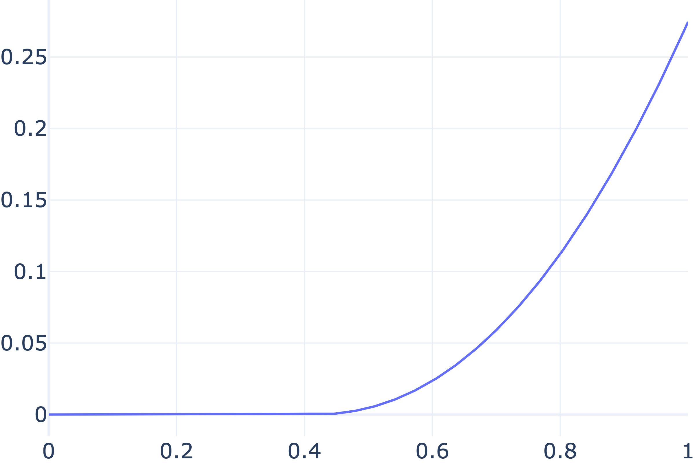
For B≥2B\geq 2 bidders, we computed how the optimal revenue depends on BB. Figure 3 depicts this dependence. Naturally, the optimal revenue is bounded from below by the revenue obtained from selling the items separately using Myerson’s optimal auction and, from above, by the revenue that the auctioneer would get if she could extract the full surplus.1313 13 Revenue of Myerson’s auction run for each item separately is 2​B​∫0.51(2​x−1)​xB−1​𝑑x2B\int_{0.5}^{1}(2x-1)x^{B-1}{\,\mathrm{d}}x while the full surplus is 2​(1−1B+1)2\left(1-\frac{1}{B+1}\right). We see that the advantage from using the optimal auction is substantial for small number of bidders and it is maximal for B=2B=2 where the optimal mechanism increases the revenue by 5.7%5.7\%. For large number of bidders, the use of optimal auction is not justified as selling the items separately leads to almost full surplus extraction.1414 14 Selling separately via optimal posted price mechanisms as well as using the optimal posted price mechanism for the grand bundle extract 1−O⁡(1B)1-O\left(\frac{1}{B}\right) fraction of the full surplus, as B→∞B\to\infty.

Refer to caption
Figure 3: Revenue as a function of the number of bidders BB for two items with i.i.d. values uniform on [0,1][0,1]. Graphs from bottom to top: selling separately (light-green), selling optimally (blue), full surplus extraction (red), limit for B→∞B\to\infty (the dashed line).

5.4.1 Algorithm

Here we describe high-level ideas behind the algorithm. The detailed description and proofs can be found in Appendix E. As discussed in the introduction, finding a solution numerically is far from being straightforward: although the auctioneer’s problem is a linear program in a functional space, any reasonable discretization of it cannot be handled by modern LP solvers because of the curse of dimensionality. Indeed, if an agent can have nn different values for each of II items, then the mechanism should specify an allocation and transfers for each of (nI)B\big(n^{I}\big)^{B} profiles of types which becomes computationally intractable already for two items, n=100n=100, and B=2B=2 agents or for n=10n=10, and B=4B=4 agents.

We escape the curse of dimensionality by dealing with the Rochet-Choné problem (11) which is equivalent to the auctioneer’s problem by Proposition 1. For nn points in the discretization, the dimension of the Rochet-Choné problem is constant in the number of bidders BB. This observation lies at the heart of algorithmic multi-to-single-agent reduction proposed (but not implemented) by Cai et al. 2012 and Alaei et al. 2019.1515 15 Comparing Figure 1 to plots obtained by Dütting et al. 2019 who did not rely multi-to-single-agent reduction, we see that even their advanced neural-network approach cannot overcome the curse of dimensionality and, as a result, is prone to smoothing artefacts. The reduction in the dimensionality comes at the cost of complexity of the feasibility constraint: the classic form of this constraint by Border 1991 leads to exponentially many inequalities and the two papers propose distinct ad hoc constructions reducing this number to polynomial.

We rely on feasibility constraint in the majorization form (12) derived by Hart and Reny 2015. It is convex but non-linear. A natural linearization is suggested by the relation between majorization and martingales well-known to economists working on information design (Blackwell 1951). We use this relation in the following form: a measure ν\nu on [0,1][0,1] majorizes ν′\nu^{\prime} if and only if there is a distribution γ\gamma on [0,1]2[0,1]^{2} with marginals ν\nu on yy and ν′\nu^{\prime} on xx and such that ∫y​𝑑γ​(y∣x)≥x\int y{\,\mathrm{d}}\gamma(y\mid x)\geq x for γ\gamma-almost all xx, where γ⁡(y∣x)\gamma(y\mid x) denotes the conditional measure on yy given xx (Shaked and Shanthikumar 2007, Theorem 4.A.5).1616 16 Equivalently, there is a supermartingale (ξ,η)(\xi,\eta) such that ξ\xi is distributed according to ν′\nu^{\prime} and η\eta, according to ν\nu.

Considering (u,γ)(u,\gamma) as unknowns, we obtain a linear optimization problem equivalent to (11). Discretization of this problem leads to a number of constraints polynomial in nn. In Appendix E, relying on duality, we demonstrate that the values of the discretized problems are guaranteed to converge to the true value as the discretization becomes finer and finer. Our approach is inspired by Ekeland and Moreno-Bromberg 2010 and, to the best of our knowledge, we are the first to obtain such approximation guarantees in multi-item auction design. To speed up the computation in practice, we adapt insights from Oberman 2013 to handle the incentive-compatibility constraint; see Appendix E for details.

The algorithm was implemented in Python using the LP solver from Gurobi library. Simulations were run on Amazon EC2 instance m6i.16xlarge with 64 vCPUs with 3rd generation Intel Xeon Scalable cores and 256 GB of memory. For n=200×200n=200\times 200 points in discretization, I=2I=2 items and B=2B=2 bidders, the computation required 83 minutes of real time and 20 hours of user time.

References

  • Adams and Hedberg (1999) D. R. Adams and L. I. Hedberg. Function Spaces and Potential Theory, volume 314 of Grundlehren der mathematischen Wissenschaften. Springer, 1999.
  • Alaei et al. (2019) S. Alaei, H. Fu, N. Haghpanah, J. Hartline, and A. Malekian. Efficient computation of optimal auctions via reduced forms. Mathematics of Operations Research, 44(3):1058–1086, 2019.
  • Aliprantis and Border (2006) C. Aliprantis and K. Border. Infinite Dimensional Analysis: A Hitchhiker’s Guide (3rd Edition). Springer Berlin Heidelberg New York, 2006.
  • Allen and Arkolakis (2014) T. Allen and C. Arkolakis. Trade and the topography of the spatial economy. The Quarterly Journal of Economics, 129(3):1085–1140, 2014.
  • Ambrosio et al. (2000) L. Ambrosio, N. Fusco, and D. Pallara. Functions of bounded variation and free discontinuity problems. Courier Corporation, 2000.
  • Arieli et al. (2019) I. Arieli, Y. Babichenko, R. Smorodinsky, and T. Yamashita. Optimal persuasion via bi-pooling. Available at SSRN 3511516, 2019.
  • Arieli et al. (2021a) I. Arieli, Y. Babichenko, F. Sandomirskiy, and O. Tamuz. Feasible joint posterior beliefs. Journal of Political Economy, 129(9):2546–2594, 2021a.
  • Arieli et al. (2021b) I. Arieli, Y. Babichenko, F. Sandomirskiy, and O. Tamuz. Persuasion as transportation. online soon, 2021b.
  • Armstrong and Rochet (1999) M. Armstrong and J.-C. Rochet. Multi-dimensional screening:: A user’s guide. European Economic Review, 43(4-6):959–979, 1999.
  • Babaioff et al. (2020) M. Babaioff, N. Immorlica, B. Lucier, and S. M. Weinberg. A simple and approximately optimal mechanism for an additive buyer. Journal of the ACM (JACM), 67(4):1–40, 2020.
  • Babaioff et al. (2021) M. Babaioff, Y. A. Gonczarowski, and N. Nisan. The menu-size complexity of revenue approximation. Games and Economic Behavior, 2021.
  • Beck (2017) A. Beck. First-order methods in optimization. SIAM, 2017.
  • Beckmann (1952) M. Beckmann. A continuous model of transportation. Econometrica: Journal of the Econometric Society, pages 643–660, 1952.
  • Bergemann et al. (2016) D. Bergemann, B. A. Brooks, and S. Morris. Informationally robust optimal auction design. 2016.
  • Bichler (2017) M. Bichler. Market design: a linear programming approach to auctions and matching. Cambridge University Press, 2017.
  • Blackwell (1951) D. Blackwell. Comparison of experiments. In Proceedings of the Second Berkeley Symposium on Mathematical Statistics and Probability, pages 93–102. University of California Press, 1951.
  • Boerma et al. (2021) J. Boerma, A. Tsyvinski, and A. P. Zimin. Sorting with team formation. Technical report, National Bureau of Economic Research, 2021.
  • Bogachev and Kolesnikov (2012) V. I. Bogachev and A. V. Kolesnikov. The Monge–Kantorovich problem: achievements, connections, and perspectives. Russian Math. Surveys, 67(5):785–890, Oct. 2012. doi: 10.1070/RM2012v067n05ABEH004808.
  • Border (1991) K. C. Border. Implementation of reduced form auctions: A geometric approach. Econometrica: Journal of the Econometric Society, pages 1175–1187, 1991.
  • Cai et al. (2012) Y. Cai, C. Daskalakis, and S. M. Weinberg. An algorithmic characterization of multi-dimensional mechanisms. In Proceedings of the forty-fourth annual ACM symposium on Theory of computing, pages 459–478, 2012.
  • Cai et al. (2019) Y. Cai, N. R. Devanur, and S. M. Weinberg. A duality-based unified approach to bayesian mechanism design. SIAM Journal on Computing, 50(3):STOC16–160, 2019.
  • Candogan and Strack (2021) O. Candogan and P. Strack. Optimal disclosure of information to a privately informed receiver. arXiv preprint arXiv:2101.10431, 2021.
  • Carlier (2012) G. Carlier. Optimal transportation and economic applications. Lecture Notes, 2012.
  • Carlier and Santambrogio (2005) G. Carlier and F. Santambrogio. A variational model for urban planning with traffic congestion. ESAIM: Control, Optimisation and Calculus of Variations, 11(4):595–613, 2005.
  • Chiappori et al. (2010) P.-A. Chiappori, R. J. McCann, and L. P. Nesheim. Hedonic price equilibria, stable matching, and optimal transport: equivalence, topology, and uniqueness. Economic Theory, 42(2):317–354, 2010.
  • Daskalakis (2015) C. Daskalakis. Multi-item auctions defying intuition? ACM SIGecom Exchanges, 14(1):41–75, 2015.
  • Daskalakis et al. (2017) C. Daskalakis, A. Deckelbaum, and C. Tzamos. Strong duality for a multiple-good monopolist. Econometrica, 85(3):735–767, 2017.
  • Dizdar and Kováč (2020) D. Dizdar and E. Kováč. A simple proof of strong duality in the linear persuasion problem. Games and Economic Behavior, 122:407–412, 2020.
  • Dütting et al. (2019) P. Dütting, Z. Feng, H. Narasimhan, D. Parkes, and S. S. Ravindranath. Optimal auctions through deep learning. In International Conference on Machine Learning, pages 1706–1715. PMLR, 2019.
  • Dworczak and Martini (2019) P. Dworczak and G. Martini. The simple economics of optimal persuasion. Journal of Political Economy, 127(5):1993–2048, 2019.
  • Ekeland and Moreno-Bromberg (2010) I. Ekeland and S. Moreno-Bromberg. An algorithm for computing solutions of variational problems with global convexity constraints. Numerische Mathematik, 115(1):45–69, 2010.
  • Fajgelbaum and Schaal (2020) P. D. Fajgelbaum and E. Schaal. Optimal transport networks in spatial equilibrium. Econometrica, 88(4):1411–1452, 2020.
  • Figalli et al. (2011) A. Figalli, Y.-H. Kim, and R. J. McCann. When is multidimensional screening a convex program? Journal of Economic Theory, 146(2):454–478, 2011.
  • Galichon (2016) A. Galichon. Optimal transport methods in economics. Princeton University Press, 2016.
  • Galichon (2021) A. Galichon. A survey of some recent applications of optimal transport methods to econometrics. arXiv preprint arXiv:2102.01716, 2021.
  • Gensbittel (2015) F. Gensbittel. Extensions of the cav (u) theorem for repeated games with incomplete information on one side. Mathematics of Operations Research, 40(1):80–104, 2015.
  • Gershkov et al. (2021) A. Gershkov, B. Moldovanu, P. Strack, and M. Zhang. A theory of auctions with endogenous valuations. Journal of Political Economy, 129(4):1011–1051, 2021.
  • Giannakopoulos and Koutsoupias (2018) Y. Giannakopoulos and E. Koutsoupias. Duality and optimality of auctions for uniform distributions. SIAM Journal on Computing, 47(1):121–165, 2018.
  • Guillen and McCann (2013) N. Guillen and R. McCann. Five lectures on optimal transportation: Geometry, regularity and applications. In Analysis and Geometry of Metric Measure Spaces: Lecture Notes of the 50th Séminaire de Mathématiques Supérieures (SMS), Montréal, 2011, chapter 6, pages 145–180. CRM Proceedings & Lecture Notes, 2013. doi: 10.1090/crmp/056/06.
  • Guo and Shmaya (2021) Y. Guo and E. Shmaya. Costly miscalibration. Theoretical Economics, 16(2):477–506, 2021.
  • Haghpanah and Hartline (2021) N. Haghpanah and J. Hartline. When is pure bundling optimal? The Review of Economic Studies, 88(3):1127–1156, 2021.
  • Hart and Nisan (2017) S. Hart and N. Nisan. Approximate revenue maximization with multiple items. Journal of Economic Theory, 172:313–347, 2017.
  • Hart and Reny (2015) S. Hart and P. J. Reny. Implementation of reduced form mechanisms: a simple approach and a new characterization. Economic Theory Bulletin, 3(1):1–8, 2015.
  • Hart and Reny (2019) S. Hart and P. J. Reny. The better half of selling separately. ACM Transactions on Economics and Computation (TEAC), 7(4):1–18, 2019.
  • Hartline (2013) J. D. Hartline. Mechanism design and approximation. Book draft, 122:1, 2013.
  • Jehiel et al. (2007) P. Jehiel, M. Meyer-Ter-Vehn, and B. Moldovanu. Mixed bundling auctions. Journal of Economic Theory, 134(1):494–512, 2007.
  • Kleiner and Manelli (2019) A. Kleiner and A. Manelli. Strong duality in monopoly pricing. Econometrica, 87(4):1391–1396, 2019.
  • Kleiner et al. (2021) A. Kleiner, B. Moldovanu, and P. Strack. Extreme points and majorization: Economic applications. Econometrica, 89(4):1557–1593, 2021.
  • Koçyiğit et al. (2020) Ç. Koçyiğit, G. Iyengar, D. Kuhn, and W. Wiesemann. Distributionally robust mechanism design. Management Science, 66(1):159–189, 2020.
  • Kolotilin (2018) A. Kolotilin. Optimal information disclosure: A linear programming approach. Theoretical Economics, 13(2):607–635, 2018.
  • Kolouri et al. (2017) S. Kolouri, S. R. Park, M. Thorpe, D. Slepcev, and G. K. Rohde. Optimal mass transport: Signal processing and machine-learning applications. IEEE Signal Processing Magazine, 34(4):43–59, 2017. doi: 10.1109/MSP.2017.2695801.
  • Manelli and Vincent (2006) A. M. Manelli and D. R. Vincent. Bundling as an optimal selling mechanism for a multiple-good monopolist. Journal of Economic Theory, 127(1):1–35, 2006.
  • Matthews (1984) S. A. Matthews. On the implementability of reduced form auctions. Econometrica: Journal of the Econometric Society, pages 1519–1522, 1984.
  • McCann and Zhang (2019) R. McCann and K. S. Zhang. On concavity of the monopolist’s problem facing consumers with nonlinear price preferences. Communication on pure and applied mathematics, 72(7):1386–1423, 2019. doi: https://doi.org/10.1002/cpa.21817.
  • Myerson (1981) R. B. Myerson. Optimal auction design. Mathematics of operations research, 6(1):58–73, 1981.
  • Myerson (2002) R. B. Myerson. Incentive-dual methods in game theory: Virtual utility and dual reduction revisited. University of Chicago (mimeo), 2002.
  • Nikzad (2022) A. Nikzad. Constrained majorization: Applications in mechanism design. Available at SSRN 4030091, 2022.
  • Nöldeke and Samuelson (2018) G. Nöldeke and L. Samuelson. The implementation duality. Econometrica, 86(4):1283–1324, 2018.
  • Oberman (2013) A. M. Oberman. A numerical method for variational problems with convexity constraints. SIAM Journal on Scientific Computing, 35(1):A378–A396, 2013.
  • Peyré and Cuturi (2019) G. Peyré and M. Cuturi. Computational optimal transport: With applications to data science. Foundations and Trends® in Machine Learning, 11(5-6):355–607, 2019. ISSN 1935-8237. doi: 10.1561/2200000073. URL http://dx.doi.org/10.1561/2200000073.
  • Rachev and Rüschendorf (2006) S. T. Rachev and L. Rüschendorf. Mass transportation problems: Applications. Springer Science & Business Media, 2006.
  • Rochet and Choné (1998) J.-C. Rochet and P. Choné. Ironing, sweeping, and multidimensional screening. Econometrica, pages 783–826, 1998.
  • Rochet and Stole (2003) J.-C. Rochet and L. A. Stole. The economics of multidimensional screening. Econometric Society Monographs, 35:150–197, 2003.
  • Rockafellar (2015) R. T. Rockafellar. Convex analysis. Princeton university press, 2015.
  • Santambrogio (2015) F. Santambrogio. Optimal transport for applied mathematicians. Birkäuser, NY, 55(58-63):94, 2015.
  • Shaked and Shanthikumar (2007) M. Shaked and J. G. Shanthikumar. Stochastic orders. Springer Science & Business Media, 2007.
  • Steinerberger and Tsyvinski (2019) S. Steinerberger and A. Tsyvinski. Tax mechanisms and gradient flows. Technical report, National Bureau of Economic Research, 2019.
  • Strassen (1965) V. Strassen. The existence of probability measures with given marginals. The Annals of Mathematical Statistics, 36(2):423–439, 1965.
  • Suzdaltsev (2020) A. Suzdaltsev. An optimal distributionally robust auction. arXiv preprint arXiv:2006.05192, 2020.
  • Villani (2009) C. Villani. Optimal transport: old and new, volume 338. Springer, 2009.
  • Vohra (2011) R. V. Vohra. Mechanism design: a linear programming approach, volume 47. Cambridge University Press, 2011.
  • Yao (2017) A. C.-C. Yao. Dominant-strategy versus bayesian multi-item auctions: Maximum revenue determination and comparison. In Proceedings of the 2017 ACM Conference on Economics and Computation, pages 3–20, 2017.

Appendix A Convex analysis basics

Throughout the paper, we consider convex functions on [0,1][0,1], XX, ℝ\mathbb{R}, or ℝℐ\mathbb{R}^{\mathcal{I}} taking values in ℝ∪{+∞}\mathbb{R}\cup\{+\infty\}. Here we briefly remind the reader some important facts and definitions.

The subdifferential of a convex function ff is defined by

∂f(x)={τ:f(y)≥f(x)+⟨τ,y−x⟩,∀y}.\partial f(x)=\{\tau:f(y)\geq f(x)+\langle\tau,\,y-x\rangle,\ \ \ \forall y\}. (40)

Partial derivatives of f⁡(x)f(x) at x∈ℝdx\in\mathbb{R}^{d} (if exist) are denoted by

fxi​(x)=∂f∂xi​(x).f_{x_{i}}(x)=\frac{\partial f}{\partial x_{i}}(x).

The gradient ∇f​(x)\nabla f(x) is the vector of partial derivatives

∇f​(x)=(fxi​(x))i=1,…,d.\nabla f(x)=\left(f_{x_{i}}(x)\right)_{i=1,\ldots,d}.

If ff is differentiable at xx, then the subdifferential ∂f⁡(x)\partial f(x) consists of just one element: ∂f⁡(x)={∇f​(x)}\partial f(x)=\{\nabla f(x)\}. By the Alexandrov theorem, a convex function is twice differentiable except for a set of zero Lebesgue measure; see (Villani 2009, Theorem 14.1). In particular, the gradient ∇f​(x)\nabla f(x) is defined almost everywhere and hence the integrals of the gradient with respect to an absolutely continuous measure are well-defined even for non-smooth ff.

The Legendre transform also known as Fenchel’s conjugate of a convex function ff is a convex function given by

f∗​(y)=supx(⟨x,y⟩−f⁡(x)).f^{*}(y)=\sup_{x}\Bigl(\langle x,y\rangle-f(x)\Bigr).

We will widely use the Fenchel inequality

f⁡(x)+f∗​(y)≥⟨x,y⟩f(x)+f^{*}(y)\geq\langle x,y\rangle (41)

and the corresponding “complementary slackness” condition taking the following form: f⁡(x)+f∗​(y)=⟨x,y⟩f(x)+f^{*}(y)=\langle x,y\rangle if and only if y∈∂f⁡(x)y\in\partial f(x) and x∈∂f∗​(y)x\in\partial f^{*}(y).

Appendix B Proof of Proposition 1 (Rochet-Choné representation of auctioneer’s problem)

Recall that the auctioneer’s problem (8) is to maximize the revenue

∫Xℬ(∑b∈ℬTb((xb)b∈ℬ))⋅(∏b∈ℬρ(xb))dx1⋯dxB\int_{X^{\mathcal{B}}}\left(\sum_{b\in\mathcal{B}}T_{b}\big((x_{b})_{b\in\mathcal{B}}\big)\right)\cdot\left(\prod_{b\in\mathcal{B}}\rho(x_{b})\right){\,\mathrm{d}}x_{1}\cdots{\,\mathrm{d}}x_{B} (42)

over individually-rational Bayesian incentive-compatible feasible mechanisms. The multi-bidder Rochet-Choné problem (11) is to maximize

B⋅∫X(⟨∇u​(x),x⟩−u⁡(x))​ρ​(x)​𝑑xB\cdot\int_{X}\Big(\langle\nabla u(x),x\rangle-u(x)\Big)\rho(x){\,\mathrm{d}}x (43)

over convex non-decreasing functions u:X→ℝ+u:\ X\to\mathbb{R}_{+} with u⁡(0)=0u(0)=0 and such that, for all i∈ℐi\in\mathcal{I},

∂u∂xi​(χ)⪯ξB−1,\frac{\partial u}{\partial x_{i}}(\chi)\preceq\xi^{B-1}, (44)

where χ∈X\chi\in X is distributed with the density ρ\rho and ξ\xi is uniformly distributed on [0,1][0,1]. Our goal is to prove that the values of the two optimization problems coincide and both maxima are attained. The proof relies on a sequence of lemmas.

It will be convenient to work with a version of the Rochet-Choné problem where the constraint u⁡(0)=0u(0)=0 is relaxed (the requirements that uu is non-decreasing and takes only non-negative values remain).

Lemma 1.

The constraint u⁡(0)=0u(0)=0 in the Rochet-Choné problem (43) can be relaxed without affecting the value and whether the optimum is attained or not.

Proof.

It is enough to show that for any feasible uu with u⁡(0)>0u(0)>0, there is a feasible u~\tilde{u} with u~​(0)=0\tilde{u}(0)=0 and the same or higher value of the objective. Defining u~​(x)=u​(x)−u​(0)\tilde{u}(x)=u(x)-u(0) completes the proof. ∎

Let us demonstrate that, for any feasible solution to (42), there is a feasible solution to (43) with the relaxed constraint u⁡(0)=0u(0)=0 and vice versa. This will imply that the two problems have the same values and, moreover, the optima are attained or not attained simultaneously.

Lemma 2.

For any individually-rational Bayesian incentive-compatible feasible mechanism (P,T)(P,T) from (42), there exists a function uu satisfying all the constraints of the Rochet-Choné problem (43) except for, possibly, u⁡(0)=0u(0)=0 and such that the revenue of (P,T)(P,T) is equal to the value of (43) at uu.

Proof.

Consider the symmetrization of the mechanism (P,T)(P,T) over all permutations of bidders:

Pb,isym​((xk)k∈ℬ)\displaystyle P_{b,i}^{\mathrm{sym}}\left((x_{k})_{k\in\mathcal{B}}\right) =1|N|!​∑σ∈SℬPσ⁡(b),i​((xσ⁡(b))b∈ℬ)\displaystyle=\frac{1}{|N|!}\sum_{\sigma\in S_{\mathcal{B}}}P_{\sigma(b),i}\left((x_{\sigma(b)})_{b\in\mathcal{B}}\right)
Tisym​((xk)k∈ℬ)\displaystyle T_{i}^{\mathrm{sym}}\left((x_{k})_{k\in\mathcal{B}}\right) =1|N|!​∑σ∈SℬTσ⁡(b)​((xσ⁡(b))b∈ℬ),\displaystyle=\frac{1}{|N|!}\sum_{\sigma\in S_{\mathcal{B}}}T_{\sigma(b)}\left((x_{\sigma(b)})_{b\in\mathcal{B}}\right),

where SℬS_{\mathcal{B}} denotes the set of all permutations σ\sigma of the set of bidders ℬ\mathcal{B}. The symmetrization (Psym,Tsym)(P^{\mathrm{sym}},T^{\mathrm{sym}}) results in the same revenue and inherits all the properties of (P,T)(P,T). By symmetry, all the bidders contribute equally to the revenue and so the revenue can be rewritten as

B⋅∫XℬT1sym((xb)b∈ℬ)⋅(∏b∈ℬρ(xb))dx1⋯dxB=B⋅∫XT1sym¯(x)⋅ρ(x)dx,B\cdot\int_{X^{\mathcal{B}}}T_{1}^{\mathrm{sym}}\big((x_{b})_{b\in\mathcal{B}}\big)\cdot\left(\prod_{b\in\mathcal{B}}\rho(x_{b})\right){\,\mathrm{d}}x_{1}\cdots{\,\mathrm{d}}x_{B}=B\cdot\int_{X}\overline{T_{1}^{\mathrm{sym}}}\big(x\big)\cdot\rho(x){\,\mathrm{d}}x,

where (P¯bsym,T¯bsym)\big(\overline{P}_{b}^{\mathrm{sym}},\,\overline{T}_{b}^{\mathrm{sym}}\big) denotes bidder bb’s reduced mechanism (reduced mechanisms are the same for all the bidders by symmetry). Define u⁡(x)u(x) as the average utility of a bidder of type x∈Xx\in X in (Psym,Tsym)(P^{\mathrm{sym}},T^{\mathrm{sym}}):

u⁡(x)=⟨P1sym¯​(x),x⟩−T1sym¯​(x).u(x)=\Big\langle\overline{P_{1}^{\mathrm{sym}}}(x),\,x\Big\rangle-\overline{T_{1}^{\mathrm{sym}}}(x).

By the definition of incentive compatibility,

⟨Pbsym¯​(y),y⟩−Tbsym¯​(y)≥⟨Pbsym¯​(x),y⟩−Tbsym¯​(x).\big\langle\overline{P_{b}^{\mathrm{sym}}}(y),\,y\big\rangle-\overline{T_{b}^{\mathrm{sym}}}(y)\geq\langle\overline{P_{b}^{\mathrm{sym}}}(x),\,y\rangle-\overline{T_{b}^{\mathrm{sym}}}(x).

Thus

u⁡(y)≥u⁡(x)+⟨P1sym¯​(x),y−x⟩.u(y)\geq u(x)+\big\langle\overline{P_{1}^{\mathrm{sym}}}(x),\ y-x\big\rangle. (45)

We conclude that u⁡(y)=maxx∈X⁡(u⁡(x)+⟨P1sym¯​(x),y−x⟩)u(y)=\max_{x\in X}\left(u(x)+\big\langle\overline{P_{1}^{\mathrm{sym}}}(x),\ y-x\big\rangle\right) and, hence, uu is a convex function as the pointwise maximum of a family of affine functions. Comparing (45) to the definition of the subdifferential of a convex function (40), we see that P1sym¯​(x)\overline{P_{1}^{\mathrm{sym}}}(x) belongs to the subdifferential ∂u⁡(x)\partial u(x). For Lebesgue-almost all xx, the gradient ∇f​(x)\nabla f(x) of a convex function ff is well-defined and the subdifferential ∂f⁡(x)\partial f(x) coincides with the singleton {∇f​(x)}\{\nabla f(x)\}. Therefore,

P1sym¯​(x)=∇u​(x)\overline{P_{1}^{\mathrm{sym}}}(x)=\nabla u(x) (46)

for almost all xx. By the definition of uu, we can express T1sym¯​(x)\overline{T_{1}^{\mathrm{sym}}}(x) as follows:

T1sym¯​(x)=⟨P1sym¯​(x),x⟩−u⁡(x)=⟨∇u​(x),x⟩−u⁡(x),\overline{T_{1}^{\mathrm{sym}}}(x)=\Big\langle\overline{P_{1}^{\mathrm{sym}}}(x),\,x\Big\rangle-u(x)=\Big\langle\nabla u(x),\,x\Big\rangle-u(x),

where the second equality holds almost everywhere. Thus

B⋅∫XT1sym¯​(x)⋅ρ⁡(x)​𝑑x=B⋅∫X(⟨∇u​(x),x⟩−u⁡(x))​ρ​(x)​𝑑x,B\cdot\int_{X}\overline{T_{1}^{\mathrm{sym}}}\big(x\big)\cdot\rho(x){\,\mathrm{d}}x=B\cdot\int_{X}\Big(\langle\nabla u(x),x\rangle-u(x)\Big)\rho(x){\,\mathrm{d}}x,

i.e., uu gives the same value to (43) as (P,T)(P,T) to (42). We already know that uu is convex. It remains to check that uu is non-negative, monotone, and that it satisfies the majorization constraint (44). Non-negativity is immediate since, by the definition, u≥0u\geq 0 is equivalent to individual rationality of (Psym,Tsym)(P^{\mathrm{sym}},T^{\mathrm{sym}}). By (46), uu is a convex function with the gradient having non-negative components almost everywhere. Hence, uu is non-decreasing.

To check (44), note that PsymP^{\mathrm{sym}} can be seen as a family of I{I} allocation rules Psym,i=(Pb,i)b∈ℬP^{\mathrm{sym},\,i}=(P_{b,i})_{b\in\mathcal{B}}, one for each item i∈ℐi\in\mathcal{I}. The reduced allocation Pbsym,i¯:X→ℝ+\overline{P_{b}^{\mathrm{sym},\,i}}\colon X\to\mathbb{R}_{+} for this one-item rule is equal to the corresponding component of Pbsym¯\overline{P_{b}^{\mathrm{sym}}}.

Hart and Reny 2015 showed that a function f:X→[0,1]f\colon X\to[0,1] coincides with a reduced form Q¯b\overline{Q}_{b} of some bidder-symmetric feasible one-item mechanism (Q,S)(Q,S) if and only if f⁡(χ)⪯ξB−1,f(\chi)\preceq\xi^{B-1}, where χ∈X\chi\in X is distributed with the density ρ\rho and ξ\xi is uniformly distributed on [0,1][0,1].

Applying this characterization, we conclude that

Pbsym,i¯​(χ)⪯ξB−1.\overline{P_{b}^{\mathrm{sym},\,i}}(\chi)\preceq\xi^{B-1}.

Since Pbsym,i¯\overline{P_{b}^{\mathrm{sym},\,i}} is equal to Pb,isym¯\overline{P_{b,i}^{\mathrm{sym}}} and the latter coincides with ∂u∂xi\frac{\partial u}{\partial x_{i}} by (46), we obtain the desired condition (44). To summarize, for any (P,T)(P,T), we constructed uu giving the same value to the Rochet-Choné problem and satisfying all its constraints (without u⁡(0)=0u(0)=0 which was shown to be redundant). ∎

Now we show how to construct (P,T)(P,T) starting from uu.

Lemma 3.

For any uu satisfying the constraints of the Rochet-Choné problem (43) except for, possibly, u⁡(0)=0u(0)=0, there exists an individually-rational Bayesian incentive-compatible feasible mechanism (P,T)(P,T) such that its revenue (42) is equal to the value of (43) at uu.

Proof.

The proof reverses the construction used to prove Lemma 2. Consider a function fif^{i} equal to the component of uu’s gradient corresponding to an item i∈ℐi\in\mathcal{I}, i.e., fi=∂u∂xif^{i}=\frac{\partial u}{\partial x_{i}}. We assume that fif^{i} is defined for all x∈Xx\in X: whenever the gradient is not well-defined, we select fif^{i} arbitrarily so that the vector f=(fi​(x))i∈ℐf=(f^{i}(x))_{i\in\mathcal{I}} belongs to the subdifferential ∂u⁡(x)\partial u(x). The function fif^{i} is non-negative as uu is monotone and f⁡(χ)f(\chi) is majorized by ξB−1\xi^{B-1} since ∂u∂xi​(χ)\frac{\partial u}{\partial x_{i}}(\chi) is. Thus, by the theorem of Hart and Reny 2015, there exists a feasible one-item allocation Pi:Xℬ→ℝ+ℬP^{i}\colon X^{\mathcal{B}}\to\mathbb{R}_{+}^{\mathcal{B}} such that Pbi¯=fi​(x)\overline{P_{b}^{i}}=f^{i}(x) for any bidder bb.

Define the mechanism (P,T)(P,T) as follows. The items are allocated by applying PiP^{i} to each i∈ℐi\in\mathcal{I}, i.e., Pb,i=PbiP_{b,i}=P_{b}^{i}. The transfers TT are given by

Tb​((xb)b∈ℬ)=⟨f⁡(xb),xb⟩−u⁡(xb).T_{b}((x_{b})_{b\in\mathcal{B}})=\big\langle f(x_{b}),x_{b}\big\rangle-u(x_{b}).

Thus (P,T)(P,T) is feasible and the reduced mechanisms satisfy

P¯b​(x)=f⁡(x)andT¯b​(x)=⟨f⁡(x),x⟩−u⁡(x)\overline{P}_{b}(x)=f(x)\quad\mbox{and}\quad\overline{T}_{b}(x)=\big\langle f(x),x\big\rangle-u(x) (47)

for any bidder bb. As f=∇uf=\nabla u almost everywhere, the second identity in (47) implies that the revenue of (P,T)(P,T) coincides with the value of (43) at uu. It remains to check that (P,T)(P,T) is individually rational and Bayesian incentive-compatible. Individual rationality reads as ⟨P¯b​(x),x⟩−T¯b​(x)≥0\langle\overline{P}_{b}(x),x\rangle-\overline{T}_{b}(x)\geq 0. By (47), the left-hand side equals u⁡(x)u(x) and so individual rationality follows from non-negativity of uu. To show incentive-compatibility, recall that f⁡(x)f(x) is an element of the subdifferential of uu and so

u⁡(x′)≥u⁡(x)+⟨f⁡(x),x′−x⟩.u(x^{\prime})\geq u(x)+\big\langle f(x),\,x^{\prime}-x\big\rangle.

By (47), this inequality rewrites as

⟨P¯b​(xb),xb⟩−T¯b​(xb)≥⟨P¯b​(xb′),xb⟩−T¯b​(xb′),\big\langle\overline{P}_{b}(x_{b}),\,x_{b}\big\rangle-\overline{T}_{b}(x_{b})\geq\langle\overline{P}_{b}(x_{b}^{\prime}),\,x_{b}\rangle-\overline{T}_{b}(x_{b}^{\prime}),

which is exactly the condition of incentive-compatibility for (P,T)(P,T). Thus (P,T)(P,T) is an individually-rational Bayesian incentive-compatible feasible mechanism with revenue equal to the value of the Rochet-Choné objective at uu. ∎

The above lemmas imply that the values of problems (42) and (43) coincide. To prove that the optima are attained we need the following pair of lemmas.

Let 𝒰Lip,1\mathcal{U}_{{\mathrm{Lip}},1} be the set of all convex non-decreasing functions u:X→ℝ+u\colon X\to\mathbb{R}_{+} with u⁡(0)=0u(0)=0 satisfying 11-Lipschitz condition |u⁡(x)−u⁡(y)|≤∑i∈ℐ|xi−yi′||u(x)-u(y)|\leq\sum_{i\in\mathcal{I}}|x_{i}-y_{i}^{\prime}| and endowed with the topology of the set of continuous functions.

Lemma 4.

The Rochet-Choné objective

B⋅∫X(⟨∇u​(x),x⟩−u⁡(x))​ρ​(x)​𝑑xB\cdot\int_{X}\Big(\langle\nabla u(x),x\rangle-u(x)\Big)\rho(x){\,\mathrm{d}}x (48)

is a continuous functional over the set 𝒰Lip,1\mathcal{U}_{{\mathrm{Lip}},1}.

Proof.

Let u(n)→uu^{(n)}\to u be a uniformly convergent sequence of functions from 𝒰Lip,1\mathcal{U}_{{\mathrm{Lip}},1}. Any limiting point yy of any sequence {y(n)}\{y^{(n)}\} such that y(n)∈∂u(n)​(x)y^{(n)}\in\partial u^{(n)}(x), belongs to ∂u⁡(x)\partial u(x). Indeed, for every zz one has

u(n)​(z)≥u(n)​(x)+⟨y(n),z−x⟩u^{(n)}(z)\geq u^{(n)}(x)+\langle y^{(n)},z-x\rangle

by definition of the subdifferential. From the convergence u(n)→uu^{(n)}\to u and y(n)→yy^{(n)}\to y one gets

u⁡(z)≥u⁡(x)+⟨y,z−x⟩u(z)\geq u(x)+\langle y,z-x\rangle

for all zz, hence, y∈∂u⁡(x)y\in\partial u(x). Since the subdifferential ∂u(n)​(x)\partial u^{(n)}(x) coincides with the gradient {∇u(n)​(x)}\{\nabla u^{(n)}(x)\} for all nn and almost all xx, we get that ∇u(n)​(x)\nabla u^{(n)}(x) converges to ∇u​(x)\nabla u(x) almost everywhere.

Thus the convergence of u(n)→uu^{(n)}\to u in the topology of continuous functions implies the convergence of integrands in (48) almost everywhere. To deduce the continuity of the functional, we need to show that taking the limit commutes with the integration. This follows from the Lebesgue dominated convergence theorem. To apply this theorem, it remains to show that, in addition to convergence almost everywhere, the sequence of integrands is bounded. Since u(n)u^{(n)} is a convergent sequence of continuous functions, supn∈ℕ,x∈X|u(n)​(x)|<∞\sup_{n\in\mathbb{N},x\in X}|u^{(n)}(x)|<\infty and ⟨∇u(n)​(x),x⟩\langle\nabla u^{(n)}(x),x\rangle is bounded by I{I} thanks to the 11-Lipschitz property. We obtain boundedness of the sequence of integrands and conclude that the Rochet-Choné objective is continuous. ∎

The next lemma shows that the feasible set in the Rochet-Choné problem is a compact subset of 𝒰Lip,1\mathcal{U}_{{\mathrm{Lip}},1}.

Lemma 5.

The set of convex non-decreasing functions u:X→ℝ+u:\ X\to\mathbb{R}_{+} with u⁡(0)=0u(0)=0 satisfying the majorization condition (44) is a compact subset of 𝒰Lip,1\mathcal{U}_{{\mathrm{Lip}},1}.

Proof.

Since the upper bound in (44) is a random variable taking values in [0,1][0,1], we see that the gradient of a function uu from the statement of the lemma takes values in [0,1]ℐ[0,1]^{\mathcal{I}} and thus such uu belongs to 𝒰Lip,1\mathcal{U}_{{\mathrm{Lip}},1}.

To prove the compactness of the set of such uu, note that the set 𝒰Lip,1\mathcal{U}_{{\mathrm{Lip}},1} is a set of uniformly bounded uniformly equicontinuous functions. Hence, any sequence of functions from 𝒰Lip,1\mathcal{U}_{{\mathrm{Lip}},1} contains a convergent subsequence. Thus, to prove compactness of a subset of 𝒰Lip,1\mathcal{U}_{{\mathrm{Lip}},1}, it is enough to check closedness of this subset. If u(n)∈𝒰Lip,1u^{(n)}\in\mathcal{U}_{{\mathrm{Lip}},1} is a sequence of functions converging uniformly to some uu, we know that their gradients ∇u(n)\nabla u^{(n)} converge to ∇u\nabla u almost surely (see the proof of Lemma 4). As the gradients are bounded, their distributions converge weakly. Therefore, if u(n)u^{(n)} satisfy the majorization condition (44), it is also satisfied by the limit uu. We obtain closedness and thus compactness. ∎

Now the proof of Proposition 1 is almost immediate.

Proof of Proposition 1.

By Lemma 1, the value of the Rochet-Choné problem does not change if we relax the constraint u⁡(0)=0u(0)=0. Lemma 2 implies that the value of the Rochet-Choné problem with the relaxed constraint is at least the value of the auctioneer’s problem, while Lemma 3 gives the opposite inequality. Thus the values of the Rochet-Choné and the auctioneer’s problems are equal.

By Lemmas 4 and 5, the Rochet-Choné problem can be seen as maximization of a continuous functional over a compact set. Therefore, this problem attains its optimum, i.e., the optimal uu exists. By Lemma 3, we can find a mechanism (P,T)(P,T) such that the auctioneer’s revenue is the same as the value of the Rochet-Choné objective. Thus the optimum in the auctioneer’s problem is also attained, i.e., the optimal auction exists as well. ∎

Appendix C Duality and proofs

In this section, we prove Theorems 1 and Theorem 2 establishing the strong dual to the auctioneer’s problem. The proof is split into two big parts. First, we derive a partial dual problem internalizing the feasibility constraint (44) of Hart and Reny 2015. This problem is interpreted as a problem of a monopolist facing adversarial production costs; a result which may be of independent interest. In terms of this problem, we formulate a novel a priori bound on solutions, our main technical tool. Next, relying on this tool, we proceed with proving the theorems.

By Proposition 1, we know that the auctioneer’s problem is equivalent to the multi-bidder Rochet-Choné problem where the distribution of uu’s gradient is majorized by a particular distribution depending on the number of bidders. As our arguments do not depend on the exact form of the dominating distribution, in this section we allow for general majorizing distributions and, consequently, the results of this section extend Theorems 1 and Theorem 2 to general majorization.

Let us describe the generalized Rochet-Choné problem and introduce some useful notation along the way. Recall that ℐ\mathcal{I} is the set of I≥1I\geq 1 items and X=[0,1]ℐX=[0,1]^{\mathcal{I}} is the set of bidders’ types endowed with a density ρ\rho. We will denote the corresponding distribution by μ\mu so that

d​μ​(x)=ρ⁡(x)​d​x{\,\mathrm{d}}\mu(x)=\rho(x){\,\mathrm{d}}x

and assume that ρ\rho is strictly positive on XX.

For a convex function uu on XX, its gradient is well-defined for almost all xx; see Appendix A. For the gradient’s component ∂∂xi​u​(x)\frac{\partial}{\partial x_{i}}u(x) we will sometimes use compact notation uxi​(x)u_{x_{i}}(x). We denote by νi\nu_{i} the distribution of the gradient’s ii’th component uxi​(χ)u_{x_{i}}(\chi) assuming that χ\chi has distribution μ\mu.

Rochet-Choné problem with general majorization: given an absolutely continuous probability measure μ\mu on XX and a collection of probability measures (ηi)i∈ℐ(\eta_{i})_{i\in\mathcal{I}} on ℝ+\mathbb{R}_{+}, maximize

∫X(⟨∇u​(x),x⟩−u⁡(x))​𝑑μ​(x)\int_{X}\Big(\langle\nabla u(x),x\rangle-u(x)\Big){\,\mathrm{d}}\mu(x) (49)

over convex non-decreasing functions u:X→ℝ+u\colon X\to\mathbb{R}_{+} with u⁡(0)=0u(0)=0 and such that for all i∈ℐi\in\mathcal{I}

νi⪯ηi,\nu_{i}\preceq\eta_{i}, (50)

where νi\nu_{i} is the distribution of uxiu_{x_{i}}.

If all ηi\eta_{i} are the same and coincide with the distribution of ξB−1\xi^{B-1} with ξ\xi uniform on [0,1][0,1], then the problem (49) coincides with the multibidder Rochet-Choné problem (11) up to a factor BB in the objective. By Proposition 1, for such choice of ηi\eta_{i}, the value of (49) is equal to 1B\frac{1}{B} of the optimal revenue in the auctioneer’s problem with BB bidders.

C.1 Auctioneer’s problem as monopolist’s problem with adversarial production costs

Consider a monopolist selling I≥1I\geq 1 items i∈ℐi\in\mathcal{I} to one buyer whose type xx is distributed according to some measure μ\mu on X=[0,1]ℐX=[0,1]^{\mathcal{I}} with density ρ\rho. In contrast to the single-bidder setting considered in Sections 2 and 3, these items have not yet been produced and so deciding on the amount to produce is a part of the monopolist’s problem. We assume that the production costs are separable across items and, for each item i∈ℐi\in\mathcal{I}, are given by a convex non-decreasing function φi\varphi_{i}. The presence of the production costs ∑i∈ℐφi​(Pi)\sum_{i\in\mathcal{I}}\varphi_{i}\big(P_{i}\big) replace the feasibility constraint Pi≤1P_{i}\leq 1 of the monopolist’s problem considered in Section 3.1. That model corresponds to a particular case of φi\varphi_{i} equal to 00 on [0,1][0,1] and +∞+\infty outside.

Monopolist’s problem with production costs. For each item i∈ℐi\in\mathcal{I}, convex non-decreasing production costs φi:[0,∞)→ℝ+∪{+∞}\varphi_{i}:\ [0,\infty)\to\mathbb{R}_{+}\cup\{+\infty\} with φi​(0)=0\varphi_{i}(0)=0 are given. The monopolist aims to maximize the total revenue consisting of the buyer’s payment minus the production costs

Φ⁡(u,(φi)i∈I)=∫X(⟨∇u​(x),x⟩−u⁡(x))​𝑑μ​(x)−∑i∈ℐ∫Xφi​(∂u∂xi​(x))​𝑑μ​(x)\Phi\big(u,(\varphi_{i})_{i\in I}\big)=\int_{X}\Big(\langle\nabla u(x),x\rangle-u(x)\Big){\,\mathrm{d}}\mu(x)-\sum_{i\in\mathcal{I}}\int_{X}\varphi_{i}\left(\frac{\partial u}{\partial x_{i}}(x)\right){\,\mathrm{d}}\mu(x) (51)

over convex non-decreasing functions u:X→ℝ+u\colon X\to\mathbb{R}_{+} with1717 17 One can show that this problem is equivalent to maximization of ∫X(T⁡(x)−∑iφi​(Pi))​𝑑μ​(x)\int_{X}(T(x)-\sum_{i}\varphi_{i}(P_{i})){\,\mathrm{d}}\mu(x) over individually-rational Bayesian incentive-compatible mechanisms (P,T):X→ℝ+ℐ×ℝ(P,T):\ X\to\mathbb{R}_{+}^{\mathcal{I}}\times\mathbb{R} (the argument repeats the proof of Proposition 1). We do not rely on this equivalence. u⁡(0)=0u(0)=0.

Let Revopt​[(φi)i∈ℐ]\mathrm{Rev}^{\mathrm{opt}}\big[(\varphi_{i})_{i\in\mathcal{I}}\big] be the value of the problem (51), i.e., the maximal revenue the monopolist can achieve. Since the zero mechanism corresponding to u≡0u\equiv 0 is feasible, the maximal revenue is non-negative, however, it may be infinite, e.g., if the costs are zero and so the monopolist has an incentive to increase production infinitely.

Consider an adversary who aims to minimize the monopolist’s revenue by selecting the production costs but is penalized for choosing high costs. The adversary’s objective is to minimize

Revopt​[(φi)i∈ℐ]+∑i∈ℐ∫φi​(z)​d​ηi​(z)\mathrm{Rev}^{\mathrm{opt}}\big[(\varphi_{i})_{i\in\mathcal{I}}\big]+\sum_{i\in\mathcal{I}}\int\varphi_{i}(z){\,\mathrm{d}}\eta_{i}(z) (52)

for some given measures ηi\eta_{i}.

Theorem 3.

Let ηi\eta_{i} be probability measures on [0,1][0,1] such that ηi​([t,1])>0\eta_{i}([t,1])>0 for any t<1t<1. Then the following assertions hold:

  • •

    The value of the Rochet-Choné problem with general majorization (49) coincides with the optimal value achieved by the adversary in the minimization problem (52).

    In particular, if all ηi\eta_{i} are equal to the the distribution of ξB−1\xi^{B-1} with ξ\xi uniformly distributed on [0,1][0,1], the value of (52) coincides with 1B\frac{1}{B} fraction of the auctioneer’s optimal revenue (8) for BB bidders.

  • •

    The optimum in (52) is attained, i.e., the adversary has an optimal strategy given by lower semicontinuous functions (φiopt)i∈ℐ(\varphi_{i}^{\mathrm{opt}})_{i\in\mathcal{I}}.

Let us formulate the result paying attention to functional classes to which uu and φi\varphi_{i} belong.

Denote by 𝒰Lip,K\mathcal{U}_{{\mathrm{Lip}},K} the set of non-decreasing convex functions uu on XX that have u⁡(0)=0u(0)=0 and are KK-Lipschitz in the l1l^{1}-norm, i.e. |u⁡(x)−u⁡(x′)|≤K​∑i|xi−xi′||u(x)-u(x^{\prime})|\leq K\sum_{i}|x_{i}-x_{i}^{\prime}|. Note that monotonicity and KK-Lipschitz properties together are equivalent to the following inequality on partial derivatives

0≤uxi≤K,∀i∈ℐ,0\leq u_{x_{i}}\leq K,\ \ \forall i\in\mathcal{I},

that must hold almost everywhere in XX. For a probability measure η\eta on [0,1][0,1], denote by 𝒰η,+∞\mathcal{U}_{\eta,+\infty} the set of convex non-decreasing lower semicontinuous functions φ:ℝ+→ℝ+∪{+∞}\varphi\colon\mathbb{R}_{+}\to\mathbb{R}_{+}\cup\{+\infty\} such that φ⁡(0)=0\varphi(0)=0, the integral ∫01φ⁡(z)​𝑑η​(z)<∞\int_{0}^{1}\varphi(z){\,\mathrm{d}}\eta(z)<\infty, and φ⁡(z)=+∞\varphi(z)=+\infty for z>1z>1.

Formally, we prove the following identity

max⁡∫u∈𝒰Lip,1,νi⪯ηi⁡(⟨x,∇u⟩−u⁡(x))​dμ==minφi∈𝒰ηi,+∞⁡maxu∈𝒰Lip,1​[Φ⁡(u,φi)+∑i∈ℐ∫01φi​(x)​d​ηi​(x)].\max_{u\in\mathcal{U}_{{\mathrm{Lip}},1},\nu_{i}\preceq\eta_{i}}\int\left(\langle x,\nabla u\rangle-u(x)\right)d\mu=\\ =\min_{\varphi_{i}\in\mathcal{U}_{\eta_{i},+\infty}}\max_{u\in\mathcal{U}_{{\mathrm{Lip}},1}}\left[\Phi(u,\varphi_{i})+\sum_{i\in\mathcal{I}}\int_{0}^{1}\varphi_{i}(x)\,{\,\mathrm{d}}\eta_{i}(x)\right]. (53)

The proof of Theorem 3 is contained in the next subsection. The high-level idea is to apply a functional minimax theorem to the Lagrangian internalizing the majorization constraint (50). Indeed, interpret Φ⁡(u,(φi)i∈ℐ)+∑i∈ℐ∫φi​(z)​d​ηi​(z)\Phi\Big(u,\,\big(\varphi_{i}\big)_{i\in\mathcal{I}}\Big)+\sum_{i\in\mathcal{I}}\int\varphi_{i}(z){\,\mathrm{d}}\eta_{i}(z) as the payoff function in a zero-sum game. The maximizer selects uu, while the minimizer picks (φi)i∈ℐ(\varphi_{i})_{i\in\mathcal{I}}. The minimizer can infinitely penalize the maximizer for a violation of the majorization constraint (50). On the other hand, if the constraint is not violated, the best the minimizer can do is to select φi≡0\varphi_{i}\equiv 0 on [0,1][0,1] for all ii making the payoff equal to the objective of the Rochet-Choné problem with general majorization (49). We conclude that the maxinf\max\inf-value of the game coincides with the value of the Rochet-Choné problem (49). Similarly, one can show that infmax\inf\max-value is the optimal value of the adversary’s problem (52). Next we apply the following functional minimax theorem which can be found in (Adams and Hedberg 1999, Theorem 2.4.1).

Theorem 4.

Let X,YX,Y be convex subsets of linear topological spaces. We assume, in addition, that XX is a compact Hausdorff space. Let f:X×Y→(−∞,+∞]f\colon X\times Y\to(-\infty,+\infty] be a function that is lower semicontinuous in xx for every y∈Yy\in Y, convex in xx, and concave in yy. Then

min⁡supy∈Yx∈X⁡f⁡(x,y)=supy∈Yminx∈X⁡f⁡(x,y).\min_{x\in X}\sup_{y\in Y}f(x,y)=\sup_{y\in Y}\min_{x\in X}f(x,y).

By this theorem, we conclude that the maxinf\max\inf and infmax\inf\max values coincide. This gives us the first item of Theorem 3. We note that, in contrast to typical game-theoretic derivations of dual problems, the payoff function Φ\Phi is not affine in the strategy uu of the maximizer. However, Φ\Phi is convex in uu which is enough for Theorem 4.

This gives the result with infimum over φi\varphi_{i} instead of minimum. Proving that the minimum is attained is the most difficult part of the proof as the set of minimizer’s strategies is not compact and so we cannot use the standard compactness arguments.

C.2 Proof of Theorem 3

In addition to 𝒰Lip,K\mathcal{U}_{{\mathrm{Lip}},K} and 𝒰η,+∞\mathcal{U}_{\eta,+\infty} defined above, we will need the following functional spaces:

  • •

    𝒰p\mathcal{U}^{p}, p≥1p\geq 1, is the set of non-decreasing convex functions u:X→ℝ+u\colon X\to\mathbb{R}_{+} with u⁡(0)=0u(0)=0 and such that ∫X|∇u|p​𝑑μ<∞\int_{X}|\nabla u|^{p}{\,\mathrm{d}}\mu<\infty, i.e., the gradient of uu belongs to Lp​(μ)L^{p}(\mu).

  • •

    𝒰ℝ+\mathcal{U}_{\mathbb{R}_{+}} is the set of convex non-decreasing lower semicontinuous functions φ:ℝ+→ℝ+∪{+∞}\varphi\colon\mathbb{R}_{+}\to\mathbb{R}_{+}\cup\{+\infty\} with φ⁡(0)=0\varphi(0)=0 such that there exists t0∈ℝ+t_{0}\in\mathbb{R}_{+} with

    φ⁡(t0)>t0.\varphi(t_{0})>t_{0}.

    Note that lower semicontinuity withing this class simply means that

    lims→t−φ⁡(s)=φ⁡(t),\lim_{s\to t-}\varphi(s)=\varphi(t),

    where t=inf{s:φ⁡(s)=+∞}t=\inf\{s:\varphi(s)=+\infty\}.

  • •

    𝒰[0,1]+∞\mathcal{U}_{[0,1]}^{+\infty} is the set of all functions φ∈𝒰ℝ+\varphi\in\mathcal{U}_{\mathbb{R}_{+}} such that φi​(t)\varphi_{i}(t) is finite for t<1t<1 and equal to +∞+\infty for t>1t>1.

The following two simple lemmas provide compactness and continuity properties needed for the proof of Theorem 3.

Lemma 6.

For any given K≥0K\geq 0, the set 𝒰Lip,K\mathcal{U}_{{\mathrm{Lip}},K} is compact in the uniform convergence topology.

Proof.

The compactness follows from the Arzelá–Ascoli theorem and the obvious fact that convexity and monotonicity are preserved under uniform convergence. ∎

The following lemma extends the continuity of the objective obtained in Lemma 4 in the presence of functions φi\varphi_{i}.

Lemma 7.

For any tuple of φi∈𝒰ℝ+\varphi_{i}\in\mathcal{U}_{\mathbb{R}_{+}} the functional Φ⁡(u,φi)\Phi(u,\varphi_{i}) is upper semicontinuous in uu in the uniform convergence topology on 𝒰Lip,K\mathcal{U}_{{\mathrm{Lip}},K} for every K>0K>0.

If, in addition, φi\varphi_{i} do not take value +∞+\infty and are continuous, then Φ⁡(u,φi)\Phi(u,\varphi_{i}) is continuous in uu in the uniform convergence topology on 𝒰Lip,K\mathcal{U}_{{\mathrm{Lip}},K} for every K>0K>0.

Proof.

As it was demonstrated in the proof of Lemma 4, if u(n)→uu^{(n)}\to u is a uniformly convergent sequence of Lipschitz convex non-decreasing functions on X{X}, then the gradients ∇u(n)\nabla u^{(n)} converge to ∇u​(x)\nabla u(x) almost everywhere. Thus, by the Fatou lemma (Theorem 11.20 in Aliprantis and Border 2006), it is sufficient to check that

limn¯​[⟨x,∇u(n)​(x)⟩−u(n)​(x)−∑i∈ℐφi​(uxi(n)​(x))]≤⟨x,∇u​(x)⟩−u⁡(x)−∑i∈ℐφi​(uxi​(x))\overline{\lim_{n}}\left[\langle x,\nabla u^{(n)}(x)\rangle-u^{(n)}(x)-\sum_{i\in\mathcal{I}}\varphi_{i}(u^{(n)}_{x_{i}}(x))\right]\leq\langle x,\nabla u(x)\rangle-u(x)-\sum_{i\in\mathcal{I}}\varphi_{i}(u_{x_{i}}(x))

μ\mu-a.e. and ⟨x,∇u(n)​(x)⟩−u(n)​(x)−∑i∈ℐφi​(uxi(n)​(x))≤C\langle x,\nabla u^{(n)}(x)\rangle-u^{(n)}(x)-\sum_{i\in\mathcal{I}}\varphi_{i}(u^{(n)}_{x_{i}}(x))\leq C for some CC. The first inequality follows immediately from μ\mu-a.e. convergence and lower semicontinuity of φi\varphi_{i}. Next, since u(n)u^{(n)}, uxi(n)u^{(n)}_{x_{i}} are nonnegative, one has

⟨x,∇u(n)​(x)⟩−u(n)​(x)−∑i∈ℐφi​(uxi(n)​(x))≤⟨x,∇u(n)​(x)⟩≤I​K.\langle x,\nabla u^{(n)}(x)\rangle-u^{(n)}(x)-\sum_{i\in\mathcal{I}}\varphi_{i}(u^{(n)}_{x_{i}}(x))\leq\langle x,\nabla u^{(n)}(x)\rangle\leq{I}K.

The second statement of the lemma follows from the Lebesgue dominated convergence theorem applied as in Lemma 4. ∎

Now we are ready to prove Theorem 3.

Proof of Theorem 3.


Step 1. The optimum in the left-hand side of (53) is attained. Indeed, by Proposition 1, we know that the value of the Rochet-Choné problem attains its value and this problem coincides with the left-hand side of (53). The proposition establishes the result for a particular choice of majorizing measures νi\nu_{i} originating from the condition by Hart and Reny 2015, but the extension to arbitrary νi\nu_{i} is straightforward.

Step 2. Let us rewrite our problem in the minimax form and apply Theorem 4:

max⁡∫u∈𝒰1,νi≤ηi⁡(⟨x,∇u⟩−u⁡(x))​𝑑μ=\displaystyle\max_{u\in\mathcal{U}^{1},\nu_{i}\leq\eta_{i}}\int\left(\langle x,\nabla u\rangle-u(x)\right)\,{\,\mathrm{d}}\mu=
=max⁡infφi∈𝒰ηi,+∞u∈𝒰Lip,1⁡[∫(⟨x,∇u⟩−u⁡(x)−∑i∈ℐφi​(uxi))​𝑑μ+∑i∈ℐ∫01φi​(x)​d​ηi​(x)]=\displaystyle=\max_{u\in\mathcal{U}_{{\mathrm{Lip}},1}}\inf_{\varphi_{i}\in\mathcal{U}_{\eta_{i},+\infty}}\left[\int\Big(\langle x,\nabla u\rangle-u(x)-\sum_{i\in\mathcal{I}}\varphi_{i}(u_{x_{i}})\Big)\,{\,\mathrm{d}}\mu+\sum_{i\in\mathcal{I}}\int_{0}^{1}\varphi_{i}(x)\,{\,\mathrm{d}}\eta_{i}(x)\right]=
=infφi∈𝒰ηi,+∞maxu∈𝒰Lip,1⁡[∫(⟨x,∇u⟩−u⁡(x)−∑i∈ℐφi​(uxi))​𝑑μ+∑i∈ℐ∫01φi​(x)​d​ηi​(x)]=\displaystyle=\inf_{\varphi_{i}\in\mathcal{U}_{\eta_{i},+\infty}}\max_{u\in\mathcal{U}_{{\mathrm{Lip}},1}}\left[\int\Big(\langle x,\nabla u\rangle-u(x)-\sum_{i\in\mathcal{I}}\varphi_{i}(u_{x_{i}})\Big)\,{\,\mathrm{d}}\mu+\sum_{i\in\mathcal{I}}\int_{0}^{1}\varphi_{i}(x)\,{\,\mathrm{d}}\eta_{i}(x)\right]=
=infφi∈𝒰ηi,+∞maxu∈𝒰Lip,1⁡[Φ⁡(u,φi)+∑i∈ℐ∫01φi​(x)​d​ηi​(x)].\displaystyle=\inf_{\varphi_{i}\in\mathcal{U}_{\eta_{i},+\infty}}\max_{u\in\mathcal{U}_{{\mathrm{Lip}},1}}\left[\Phi(u,\varphi_{i})+\sum_{i\in\mathcal{I}}\int_{0}^{1}\varphi_{i}(x)\,{\,\mathrm{d}}\eta_{i}(x)\right].

The first equality is obvious, while the second one follows from the minimax principle. Here we use compactness of 𝒰Lip,1\mathcal{U}_{{\mathrm{Lip}},1}, linearity in φi\varphi_{i}, concavity in uu (follows from convexity of φi\varphi_{i}), the upper semicontinuity was established in Theorem 2.

Step 3. We construct such a family of functions (φi)(\varphi_{i}) that the infimum in the right-hand side of (53) is prospectively reached on them. Consider a sequence of tuples of functions {(φi(n))i∈ℐ}n⊂𝒰ηi,+∞\{(\varphi_{i}^{(n)})_{i\in\mathcal{I}}\}_{n}\subset\mathcal{U}_{\eta_{i},+\infty} such that

limn→∞maxu∈𝒰Lip,1⁡[Φ⁡(u,φi(n))+∑i∈ℐ∫01φi(n)​(x)​d​ηi​(x)]==max⁡∫u∈𝒰1,νi⪯ηi⁡(⟨x,∇u⟩−u⁡(x))​dμ.\lim_{n\to\infty}\max_{u\in\mathcal{U}_{{\mathrm{Lip}},1}}\left[\Phi(u,\varphi_{i}^{(n)})+\sum_{i\in\mathcal{I}}\int_{0}^{1}\varphi_{i}^{(n)}(x)\,{\,\mathrm{d}}\eta_{i}(x)\right]=\\ =\max_{u\in\mathcal{U}^{1},\nu_{i}\preceq\eta_{i}}\int(\langle x,\nabla u\rangle-u(x))\,{\,\mathrm{d}}\mu. (54)

Denote by MM the optimal value of the objective function

M=max⁡∫u∈𝒰1,νi⪯ηi⁡(⟨x,∇u⟩−u⁡(x))​𝑑μ.M=\max_{u\in\mathcal{U}^{1},\nu_{i}\preceq\eta_{i}}\int(\langle x,\nabla u\rangle-u(x))\,{\,\mathrm{d}}\mu.

We may assume that for all nn we have

2​M≥maxu∈𝒰Lip,1⁡[Φ⁡(u,φi(n))+∑i∈ℐ∫01φi(n)​(x)​d​ηi​(x)].2M\geq\max_{u\in\mathcal{U}_{{\mathrm{Lip}},1}}\left[\Phi(u,\varphi_{i}^{(n)})+\sum_{i\in\mathcal{I}}\int_{0}^{1}\varphi_{i}^{(n)}(x)\,{\,\mathrm{d}}\eta_{i}(x)\right].

Since maxu∈𝒰Lip,1⁡Φ⁡(u,φi(n))≥0\max_{u\in\mathcal{U}_{{\mathrm{Lip}},1}}\Phi(u,\varphi_{i}^{(n)})\geq 0 and φi(n)​(x)≥0\varphi_{i}^{(n)}(x)\geq 0 for all xx, we conclude that ∫01φi(n)​(x)​d​ηi≤2​M\int_{0}^{1}\varphi_{i}^{(n)}(x)\,{\,\mathrm{d}}\eta_{i}\leq 2M for all i∈ℐ{i\in\mathcal{I}} and for all nn. All the functions φi(n)\varphi_{i}^{(n)} are non-negative and non-decreasing on [0,1][0,1]; therefore, for every t∈[0,1)t\in[0,1),

∫01φi(n)​(x)​d​ηi≥∫t1φi(n)​(x)​d​ηi≥φi(n)​(t)⋅ηi​([t,1]).\int_{0}^{1}\varphi_{i}^{(n)}(x)\,{\,\mathrm{d}}\eta_{i}\geq\int_{t}^{1}\varphi_{i}^{(n)}(x)\,{\,\mathrm{d}}\eta_{i}\geq\varphi_{i}^{(n)}(t)\cdot\eta_{i}([t,1]).

Thus φi(n)​(t)≤Mt\varphi_{i}^{(n)}(t)\leq M_{t} for all t∈[0,1)t\in[0,1) and for all nn, where Mt=2​M/ηi​([t,1])M_{t}=2M/\eta_{i}([t,1]).

For every t∈[0,1)t\in[0,1), the sequence {φi(n)}\{\varphi_{i}^{(n)}\} is uniformly bounded on [0,t][0,t] by the constant MtM_{t}. So, applying Helly’s principle and passing to subsequences countably many number of times, we can assume that there exists a tuple of functions (φi)i∈ℐ(\varphi_{i})_{i\in\mathcal{I}} defined on [0,1)[0,1) such that φi(n)→φi\varphi_{i}^{(n)}\to\varphi_{i} pointwise on [0,1)[0,1).

Each of the functions φi\varphi_{i} is non-negative, non-decreasing, and convex. In particular, limt→1−φi​(t)\lim_{t\to 1-}\varphi_{i}(t) is well defined. We extend the definition of φi\varphi_{i} on [0,+∞)[0,+\infty) as follows: define φi​(1)\varphi_{i}(1) as limt→1−φi​(t)∈ℝ∪{+∞}\lim_{t\to 1-}\varphi_{i}(t)\in\mathbb{R}\cup\{+\infty\}, and define φi​(x)\varphi_{i}(x) at every x∈(1,+∞)x\in(1,+\infty) to be equal to +∞+\infty. The constructed function is lower-semicontinuous. Besides, limn→∞φi(n)​(x)=φi​(x)\lim_{n\to\infty}\varphi_{i}^{(n)}(x)=\varphi_{i}(x) for all x∈[0,1)x\in[0,1), and one can easily check that lim infn→∞φi(n)​(1)≥φi​(1)\liminf_{n\to\infty}\varphi_{i}^{(n)}(1)\geq\varphi_{i}(1).

We only need to check that φi∈L1​(ηi)\varphi_{i}\in L^{1}(\eta_{i}) to prove that φi∈𝒰ηi,+∞\varphi_{i}\in\mathcal{U}_{\eta_{i},+\infty}. For every ii, the sequence of integrals {∫01φi(n)​(x)​d​ηi}n\{\int_{0}^{1}\varphi_{i}^{(n)}(x)\,{\,\mathrm{d}}\eta_{i}\}_{n} is bounded. Passing to subsequences, we may additionally assume (and we will use it in the following part of the proof) that each of this sequences converges. By the Fatou lemma,

2​M≥limn→∞∫01φi(n)​(x)​d​ηi≥∫01lim infn→∞φi(n)​(x)​d​ηi≥∫01φi​(x)​d​ηi.2M\geq\lim_{n\to\infty}\int_{0}^{1}\varphi_{i}^{(n)}(x)\,{\,\mathrm{d}}\eta_{i}\geq\int_{0}^{1}\liminf_{n\to\infty}\varphi_{i}^{(n)}(x)\,{\,\mathrm{d}}\eta_{i}\geq\int_{0}^{1}\varphi_{i}(x)\,{\,\mathrm{d}}\eta_{i}. (55)

Hence, φi∈L1​(ηi)\varphi_{i}\in L^{1}(\eta_{i}). Thus φi∈𝒰ηi,+∞\varphi_{i}\in\mathcal{U}_{\eta_{i},+\infty}.

Step 4. We claim that for all u∈𝒰Lip,1u\in\mathcal{U}_{{\mathrm{Lip}},1} the following inequality holds:

Φ⁡(u,φi)+∑i∈ℐ∫01φi​(x)​d​ηi​(x)≤M.\Phi(u,\varphi_{i})+\sum_{i\in\mathcal{I}}\int_{0}^{1}\varphi_{i}(x)\,{\,\mathrm{d}}\eta_{i}(x)\leq M.

Fix a function u∈𝒰Lip,1u\in\mathcal{U}_{{\mathrm{Lip}},1}. For any ε∈(0,1)\varepsilon\in(0,1), consider a function uε=(1−ε)⋅u∈𝒰Lip,1−εu^{\varepsilon}=(1-\varepsilon)\cdot u\in\mathcal{U}_{{\mathrm{Lip}},1-\varepsilon}. For all x∈Xx\in{X} and for all i∈ℐ{i\in\mathcal{I}}, the value uxiε​(x)u^{\varepsilon}_{x_{i}}(x) is not greater than 1−ε1-\varepsilon. So, for any i∈ℐ{i\in\mathcal{I}}, the sequence of functions {φi(n)​(uxiε​(x))}n\{\varphi_{i}^{(n)}(u^{\varepsilon}_{x_{i}}(x))\}_{n} converges to φi​(uxiε​(x))\varphi_{i}(u^{\varepsilon}_{x_{i}}(x)) pointwise almost everywhere. In addition, the inequality 0≤φi(n)​(uxiε​(x))≤M1−ε0\leq\varphi_{i}^{(n)}(u^{\varepsilon}_{x_{i}}(x))\leq M_{1-\varepsilon} holds for almost all x∈Xx\in{X} and for all nn; therefore, it follows from Lebesgue’s dominated convergence theorem that

limn→∞∫φi(n)​(uxiε)​𝑑μ=∫φi​(uxiε)​𝑑μ.\lim_{n\to\infty}\int\varphi_{i}^{(n)}(u^{\varepsilon}_{x_{i}})\,{\,\mathrm{d}}\mu=\int\varphi_{i}(u^{\varepsilon}_{x_{i}})\,{\,\mathrm{d}}\mu.

Combining this with the fact that limn→∞∫01φi(n)​(x)​d​ηi≥∫01φi​(x)​d​ηi\lim_{n\to\infty}\int_{0}^{1}\varphi_{i}^{(n)}(x)\,{\,\mathrm{d}}\eta_{i}\geq\int_{0}^{1}\varphi_{i}(x)\,{\,\mathrm{d}}\eta_{i}, we conclude that

limn→∞[Φ⁡(uε,φi(n))+∑i∈ℐ∫01φi(n)​(x)​d​ηi​(x)]≥Φ⁡(uε,φi)+∑i∈ℐ∫01φi​(x)​d​ηi​(x).\lim_{n\to\infty}\left[\Phi\left(u^{\varepsilon},\varphi_{i}^{(n)}\right)+\sum_{i\in\mathcal{I}}\int_{0}^{1}\varphi_{i}^{(n)}(x)\,{\,\mathrm{d}}\eta_{i}(x)\right]\geq\Phi(u^{\varepsilon},\varphi_{i})+\sum_{i\in\mathcal{I}}\int_{0}^{1}\varphi_{i}(x)\,{\,\mathrm{d}}\eta_{i}(x).

In particular,

M\displaystyle M =limn→∞maxv∈𝒰Lip,1⁡[Φ⁡(v,φi(n))+∑i∈ℐ∫01φi(n)​(x)​d​ηi​(x)]≥\displaystyle=\lim_{n\to\infty}\max_{v\in\mathcal{U}_{{\mathrm{Lip}},1}}\left[\Phi\left(v,\varphi_{i}^{(n)}\right)+\sum_{i\in\mathcal{I}}\int_{0}^{1}\varphi_{i}^{(n)}(x)\,{\,\mathrm{d}}\eta_{i}(x)\right]\geq
≥limn→∞[Φ⁡(uε,φi(n))+∑i∈ℐ∫01φi(n)​(x)​d​ηi​(x)]≥\displaystyle\geq\lim_{n\to\infty}\left[\Phi\left(u^{\varepsilon},\varphi_{i}^{(n)}\right)+\sum_{i\in\mathcal{I}}\int_{0}^{1}\varphi_{i}^{(n)}(x)\,{\,\mathrm{d}}\eta_{i}(x)\right]\geq
≥Φ⁡(uε,φi)+∑i∈ℐ∫01φi​(x)​d​ηi​(x).\displaystyle\geq\Phi(u^{\varepsilon},\varphi_{i})+\sum_{i\in\mathcal{I}}\int_{0}^{1}\varphi_{i}(x)\,{\,\mathrm{d}}\eta_{i}(x).

Let εn=1n\varepsilon_{n}=\frac{1}{n}. For every i∈ℐ{i\in\mathcal{I}}, the sequence {φi​(uxiεn​(x))}n\{\varphi_{i}(u_{x_{i}}^{\varepsilon_{n}}(x))\}_{n} is an increasing sequence of non-negative functions that converges to φi​(uxi​(x))\varphi_{i}(u_{x_{i}}(x)) pointwise. So, by the Beppo Levi’s lemma (Theorem 11.18 in Aliprantis and Border 2006) we have

limn→∞∫φi​(uxiεn​(x))​𝑑μ​(x)=∫φi​(uxi​(x))​𝑑μ​(x).\lim_{n\to\infty}\int\varphi_{i}(u_{x_{i}}^{\varepsilon_{n}}(x))\,{\,\mathrm{d}}\mu(x)=\int\varphi_{i}(u_{x_{i}}(x))\,{\,\mathrm{d}}\mu(x).

Thus, for all u∈𝒰Lip,1u\in\mathcal{U}_{{\mathrm{Lip}},1}, we have

Φ⁡(u,φi)+∑i∈ℐ∫01φi​(x)​d​ηi​(x)=limn→∞(Φ⁡(uεn,φi)+∑i∈ℐ∫01φi​(x)​d​ηi​(x))≤M.\Phi(u,\varphi_{i})+\sum_{i\in\mathcal{I}}\int_{0}^{1}\varphi_{i}(x)\,{\,\mathrm{d}}\eta_{i}(x)=\lim_{n\to\infty}\left(\Phi(u^{\varepsilon_{n}},\varphi_{i})+\sum_{i\in\mathcal{I}}\int_{0}^{1}\varphi_{i}(x)\,{\,\mathrm{d}}\eta_{i}(x)\right)\leq M.

Since the last inequality holds for all u∈𝒰Lip,1u\in\mathcal{U}_{{\mathrm{Lip}},1}, we conclude that

maxu∈𝒰Lip,1⁡[Φ⁡(u,φi)+∑i∈ℐ∫01φi​(x)​d​ηi​(x)]≤M.\max_{u\in\mathcal{U}_{{\mathrm{Lip}},1}}\left[\Phi(u,\varphi_{i})+\sum_{i\in\mathcal{I}}\int_{0}^{1}\varphi_{i}(x)\,{\,\mathrm{d}}\eta_{i}(x)\right]\leq M.

Thus it follows from the definition of MM that the equality holds and the minimum in (53) is reached on a family of functions sequence of functions (φi)i∈ℐ(\varphi_{i})_{i\in\mathcal{I}}. ∎

C.3 Tools to approach complete duality: main a priori estimate and its corollaries

In the next section, we discuss the complete duality results. The main insight allowing us to cope with non-compactness of the problem is an a priori bound on a solution. This bound has a clear economic interpretation in the context of the monopolist’s problem with production (51). Here we discuss this bound and its implications.

Informally, the bound is as follows. It states that in the optimal mechanism, the monopolist never gets a negative revenue ex-post, i.e., ⟨∇uopt​(x),x⟩−uopt​(x)−∑i∈ℐφi​(uxiopt​(x))\langle\nabla u^{\mathrm{opt}}(x),x\rangle-u^{\mathrm{opt}}(x)-\sum_{i\in\mathcal{I}}\varphi_{i}(u_{x_{i}}^{\mathrm{opt}}(x)) is non-negative.1818 18 Formulated in terms of monopolist’s mechanism (Popt,Topt)(P^{\mathrm{opt}},T^{\mathrm{opt}}), this inequality means Topt​(x)−∑i∈ℐφi​(Piopt​(x))≥0.T^{\mathrm{opt}}(x)-\sum_{i\in\mathcal{I}}\varphi_{i}\big(P_{i}^{\mathrm{opt}}(x)\big)\geq 0. This observation is not elementary as one could possibly expect that by serving those costumers who bring negative profit, the monopolist could extract higher rent from the rest of the population.

We will rely on the notation for functional classes introduced in Section C.2.

Proposition 3.

(Main a priori estimate). Let (φi)i∈I(\varphi_{i})_{i\in I} be a collection of functions from 𝒰ℝ+\mathcal{U}_{\mathbb{R}_{+}}. Then for every function u∈𝒰1u\in\mathcal{U}^{1}, there exists a non-decreasing convex function u~\tilde{u} with u~​(0)=0\tilde{u}(0)=0 such that

⟨x,∇u~​(x)⟩−u~​(x)−∑i∈ℐφi​(u~xi​(x))≥max⁡{⟨x,∇u​(x)⟩−u⁡(x)−∑i∈ℐφi​(uxi​(x)), 0}\langle x,\nabla\tilde{u}(x)\rangle-\tilde{u}(x)-\sum_{i\in\mathcal{I}}\varphi_{i}(\tilde{u}_{x_{i}}(x))\geq\max\left\{\langle x,\nabla u(x)\rangle-u(x)-\sum_{i\in\mathcal{I}}\varphi_{i}(u_{x_{i}}(x)),\,0\right\} (56)

for all x∈Xx\in X. In particular, this implies (see Proposition 4) that for any function uopt∈𝒰1u^{\mathrm{opt}}\in\mathcal{U}^{1} maximizing the functional Φ⁡(u,φi)\Phi(u,\varphi_{i}) over u∈𝒰1u\in\mathcal{U}^{1}, the inequality

⟨x,∇uopt​(x)⟩−uopt​(x)−∑i∈ℐφi​(uxiopt​(x))≥0\langle x,\nabla{u^{\mathrm{opt}}}(x)\rangle-{u^{\mathrm{opt}}}(x)-\sum_{i\in\mathcal{I}}\varphi_{i}\left(u_{x_{i}}^{\mathrm{opt}}(x)\right)\geq 0 (57)

holds almost everywhere.

The main a priori estimate is used in Proposition 4 to show that, for a wide class of functions φi\varphi_{i}, the functional Φ⁡(u,φi)\Phi(u,\varphi_{i}) attains its maximum on a Lipshitz function uu. This fact will be used in approximation Lemma 8 which, together with Proposition 6, help us to justify the minimax principle (Proposition 6) needed to prove complete duality (Theorem 5).

Proof of Proposition 3.

Consider the Legendre transform of uu

u∗​(y)=supx(⟨x,y⟩−u⁡(x)),u^{*}(y)=\sup_{x}(\langle x,y\rangle-u(x)),

assuming u⁡(x)=+∞u(x)=+\infty if x∉Xx\notin{X}. Next we define

v⁡(y)=max⁡{u∗​(y),∑i∈ℐφi​(yi)}.v(y)=\max\left\{u^{*}(y),\sum_{i\in\mathcal{I}}\varphi_{i}(y_{i})\right\}.

Note that vv is a lower semicontinuous convex function and v⁡(0)=0v(0)=0. Set

u~=v∗=[max⁡{u∗,∑i∈ℐφi}]∗.\tilde{u}=v^{*}=\left[\max\left\{u^{*},\sum_{i\in\mathcal{I}}\varphi_{i}\right\}\right]^{*}.

Then, by the Fenchel–Moreau theorem (Rockafellar 2015),

(u~)∗=max⁡{u∗,∑i∈ℐφi}(\tilde{u})^{*}=\max\left\{u^{*},\sum_{i\in\mathcal{I}}\varphi_{i}\right\}

and, for every point xx where ∇u~​(x)\nabla\tilde{u}(x) exists, one has

⟨x,∇u~​(x)⟩−u~​(x)−∑i∈ℐφi​(u~xi)=((u~)∗−∑i∈ℐφi)​(∇u~)≥0.\langle x,\nabla\tilde{u}(x)\rangle-\tilde{u}(x)-\sum_{i\in\mathcal{I}}\varphi_{i}(\tilde{u}_{x_{i}})=\left((\tilde{u})^{*}-\sum_{i\in\mathcal{I}}\varphi_{i}\right)(\nabla\tilde{u})\geq 0. (58)

Consider a point xx, such that ∇u​(x)\nabla u(x) exists and satisfies ⟨x,∇u​(x)⟩−u⁡(x)−∑i∈ℐφi​(uxi​(x))≥0\langle x,\nabla u(x)\rangle-u(x)-\sum_{i\in\mathcal{I}}\varphi_{i}(u_{x_{i}}(x))\geq 0. Equivalently, (u∗−∑i∈ℐφi)​(∇u​(x))≥0(u^{*}-\sum_{i\in\mathcal{I}}\varphi_{i})(\nabla u(x))\geq 0. It follows from the theorem about the subdifferential of a maximum of convex functions (Dubovitsky-Milyutin theorem; see Theorem 3.50 in Beck 2017) that ∂v⁡(y)=∂[max⁡{u∗,∑i∈ℐφi}]​(y)\partial v(y)=\partial\left[\max\left\{u^{*},\sum_{i\in\mathcal{I}}\varphi_{i}\right\}\right](y) contains ∂u∗​(y)\partial u^{*}(y) if u∗≥∑i∈ℐφiu^{*}\geq\sum_{i\in\mathcal{I}}\varphi_{i}. Hence, if xx satisfies (u∗−∑i∈ℐφi)​(∇u​(x))≥0(u^{*}-\sum_{i\in\mathcal{I}}\varphi_{i})(\nabla u(x))\geq 0, then

v⁡(∇u​(x))=u∗​(∇(x))andx∈∂v⁡(∇u​(x)).v(\nabla u(x))=u^{*}(\nabla(x))\quad{\rm and}\quad x\in\partial v(\nabla u(x)).

This implies v⁡(∇u​(x))+v∗​(x)=⟨∇u​(x),x⟩v(\nabla u(x))+v^{*}(x)=\langle\nabla u(x),x\rangle, hence

u~​(x)=v∗​(x)=⟨∇u​(x),x⟩−u∗​(∇u​(x))=u⁡(x)\tilde{u}(x)=v^{*}(x)=\langle\nabla u(x),x\rangle-u^{*}(\nabla u(x))=u(x)

and from the inclusion x∈∂v​(∇u​(x))x\in\partial v(\nabla u(x)) we get ∇u​(x)∈∂v∗​(x)=∂u~​(x)\nabla u(x)\in\partial v^{*}(x)=\partial\tilde{u}(x). In particular, if ∇u~\nabla{\tilde{u}} exists, then ∇u​(x)=∇u~​(x)\nabla u(x)=\nabla\tilde{u}(x) and

⟨x,∇u~​(x)⟩−u~​(x)−∑i∈ℐφi​(u~xi)=⟨x,∇u​(x)⟩−u⁡(x)−∑i∈ℐφi​(uxi).\langle x,\nabla\tilde{u}(x)\rangle-\tilde{u}(x)-\sum_{i\in\mathcal{I}}\varphi_{i}(\tilde{u}_{x_{i}})=\langle x,\nabla{u}(x)\rangle-{u}(x)-\sum_{i\in\mathcal{I}}\varphi_{i}({u}_{x_{i}}). (59)

The desired inequality (56) follows from (58) and (59). ∎

With the help of the main a priori estimate, we obtain the following a priori bound on the regularity of the optimum.

Proposition 4.

Fix a collection of functions φi∈𝒰ℝ+\varphi_{i}\in\mathcal{U}_{\mathbb{R}_{+}}, i∈ℐi\in\mathcal{I}, and consider numbers MiM_{i} such that

φi​(Mi)>Mi,\varphi_{i}(M_{i})>M_{i},

which exist by the definition of the class 𝒰ℝ+\mathcal{U}_{\mathbb{R}_{+}}. Then there exists a number LL depending on MiM_{i} and φi​(Mi)\varphi_{i}(M_{i}) such that Φ⁡(u,φi)\Phi(u,\varphi_{i}) attains its maximum on 𝒰1\mathcal{U}^{1} at a function uopt{u^{\mathrm{opt}}} that belongs to 𝒰Lip,L\mathcal{U}_{{\mathrm{Lip}},L}.

Proof.

By Proposition 3, any function v∈𝒰1v\in\mathcal{U}^{1} can be replaced with a convex non-decreasing function uu with u⁡(0)=0u(0)=0 such that

Φ⁡(u,φi)≥Φ⁡(v,φi)\displaystyle\Phi(u,\varphi_{i})\geq\Phi(v,\varphi_{i}) (60)
and
⟨x,∇u​(x)⟩−u⁡(x)−∑i∈ℐφi​(uxi​(x))≥0\displaystyle\langle x,\nabla u(x)\rangle-u(x)-\sum_{i\in\mathcal{I}}\varphi_{i}(u_{x_{i}}(x))\geq 0 (61)

for almost all xx. Moreover, if the function vv does not satisfy inequality (61), then (60) is strict. So, it is enough to check the existence of LL depending on φi\varphi_{i}, such that every Lipschitz function uu satisfying this inequality is LL-Lipschitz.

Indeed, since u⁡(x)≥0u(x)\geq 0, uxi​(x)≥0u_{x_{i}}(x)\geq 0 and xi≤1x_{i}\leq 1 for all i∈ℐ{i\in\mathcal{I}}, assumption (61) implies:

ux1+ux2+⋯+uxI−∑i∈ℐφi​(uxi)≥≥⟨x,∇u​(x)⟩−u⁡(x)−∑i∈ℐφi​(uxi)≥0.\displaystyle\begin{split}u_{x_{1}}+u_{x_{2}}+\cdots+u_{x_{I}}-&\sum_{i\in\mathcal{I}}\varphi_{i}(u_{x_{i}})\geq\\ \geq\langle x,\nabla u(x)\rangle-u(x)-&\sum_{i\in\mathcal{I}}\varphi_{i}(u_{x_{i}})\geq 0.\end{split} (62)

For all i∈ℐi\in\mathcal{I}, consider function ψi​(xi)=xi−φi​(xi)\psi_{i}(x_{i})=x_{i}-\varphi_{i}(x_{i}). This function is concave and 0=ψi​(0)>ψi​(Mi)0=\psi_{i}(0)>\psi_{i}(M_{i}). Hence, ψi\psi_{i} is decreasing on [Mi,+∞)[M_{i},+\infty) and its maximum is reached on [0,Mi][0,M_{i}]. Note that ψi​(xi)≤xi\psi_{i}(x_{i})\leq x_{i} for all xix_{i}, hence

maxx≥0⁡ψi​(xi)=max0≤xi≤Mi⁡ψi​(xi)≤Mi.\max_{x\geq 0}\psi_{i}(x_{i})=\max_{0\leq x_{i}\leq M_{i}}\psi_{i}(x_{i})\leq M_{i}.

Inequality (62) can be rewritten in the following form:

∑i∈ℐψi​(uxi​(xi))≥0\sum_{i\in\mathcal{I}}\psi_{i}(u_{x_{i}}(x_{i}))\geq 0

for almost all x∈Xx\in{X}. Hence, for all i∈ℐ{i\in\mathcal{I}} and almost all x∈Xx\in{X},

ψi(uxi(xi))≥−∑j≠iψj(uxj(xj))≥−∑j≠iMj.\psi_{i}(u_{x_{i}}(x_{i}))\geq-\sum_{j\neq i}\psi_{j}(u_{x_{j}}(x_{j}))\geq-\sum_{j\neq i}M_{j}. (63)

Concavity of ψi\psi_{i} implies that all xi≥Mix_{i}\geq M_{i} satisfy inequality

ψi​(xi)−ψi​(Mi)xi−Mi≤ψi′(Mi)≤ψi​(Mi)−ψi​(0)Mi−0⇔ψi(xi)≤xMiψi(Mi).\frac{\psi_{i}(x_{i})-\psi_{i}(M_{i})}{x_{i}-M_{i}}\leq\psi^{\prime}_{i}(M_{i})\leq\frac{\psi_{i}(M_{i})-\psi_{i}(0)}{M_{i}-0}\quad\Leftrightarrow\quad\psi_{i}(x_{i})\leq\frac{x}{M_{i}}\psi_{i}(M_{i}).

Hence, if

xi>max⁡{Mi,−∑j≠iMj⋅Miψi​(Mi)}=M^i,x_{i}>\max\left\{M_{i},-\frac{\sum_{j\neq i}M_{j}\cdot M_{i}}{\psi_{i}(M_{i})}\right\}=\widehat{M}_{i},

then ψi(xi)<−∑i∈ℐMi\psi_{i}(x_{i})<-\sum_{i\in\mathcal{I}}M_{i}.

Hence, inequality (63) implies that uxi​(x)≤M^iu_{x_{i}}(x)\leq\widehat{M}_{i} for almost all xx. Thus uu is LL-Lipschitz with L=max⁡{M^i}L=\max\left\{\widehat{M}_{i}\right\}.

It remains to show that Φ⁡(u,φi)\Phi(u,\varphi_{i}) attains its maximum on 𝒰Lip,L\mathcal{U}_{{\mathrm{Lip}},L}.

According to estimate (57) we can restrict ourselves to the set of functions u∈𝒰1u\in\mathcal{U}^{1} satisfying

⟨x,∇u​(x)⟩−u⁡(x)−∑i∈ℐφi​(uxi​(x))≥0\displaystyle\langle x,\nabla u(x)\rangle-u(x)-\sum_{i\in\mathcal{I}}\varphi_{i}(u_{x_{i}}(x))\geq 0

for almost all x∈Xx\in{X}. We showed that all such functions uu belong to 𝒰Lip,L\mathcal{U}_{{\mathrm{Lip}},L}. This set is compact in uniform convergence topology and Φ⁡(u,φi)\Phi(u,\varphi_{i}) upper semicontinuous on 𝒰Lip,L\mathcal{U}_{{\mathrm{Lip}},L}. Hence, it reaches its maximum on this set. ∎

To prove complete duality, we will need the following weak form of partial duality. The goal is to represent the value in the infmax\inf\max form so that we can apply the miminax theorem and obtain the maxinf\max\inf representation, which is done in Proposition 6. The subtlety is that, to apply the minimax theorem, compactness of one of the spaces is required and so we need to choose carefully a dense minimization subspace 𝒬\mathcal{Q} in the set of convex one-dimensional functions. In what follows,

𝒬⊂𝒰ℝ+\mathcal{Q}\subset\mathcal{U}_{\mathbb{R}_{+}} (64)

denotes the set of all increasing, convex functions φ:[0,+∞)→ℝ+\varphi\colon[0,+\infty)\to\mathbb{R}_{+} that equal zero at the origin and have bounded derivatives.

Proposition 5.

Under the assumptions of Theorem 3, the following partial duality equation holds:

max⁡∫u∈𝒰Lip,1,νi⪯ηi⁡(⟨x,∇u⟩−u⁡(x))​𝑑μ=infφi∈𝒬maxu∈𝒰1⁡[Φ⁡(u,φi)+∑i∈ℐ∫01φi​(x)​d​ηi​(x)].\max_{u\in\mathcal{U}_{{\mathrm{Lip}},1},\nu_{i}\preceq\eta_{i}}\int\left(\langle x,\nabla u\rangle-u(x)\right)d\mu=\inf_{\varphi_{i}\in\mathcal{Q}}\max_{u\in\mathcal{U}^{1}}\left[\Phi(u,\varphi_{i})+\sum_{i\in\mathcal{I}}\int_{0}^{1}\varphi_{i}(x)\,{\,\mathrm{d}}\eta_{i}(x)\right].

The key part of the proof is the following lemma.

Lemma 8.

For any family of functions (φi)i∈ℐ⊂𝒰[0,1]+∞(\varphi_{i})_{i\in\mathcal{I}}\subset\mathcal{U}_{[0,1]}^{+\infty} there exist increasing sequences of functions {φi(n)}n⊂𝒬\{\varphi_{i}^{(n)}\}_{n}\subset\mathcal{Q}, i∈ℐ{i\in\mathcal{I}}, such that each sequence {φi(n)}n\{\varphi_{i}^{(n)}\}_{n} converges to φi\varphi_{i} pointwise on [0,1][0,1] and that

maxu∈𝒰Lip,1⁡Φ⁡(u,φi)=limn→∞maxu∈𝒰1⁡Φ⁡(u,φi(n)).\max_{u\in\mathcal{U}_{{\mathrm{Lip}},1}}\Phi(u,\varphi_{i})=\lim_{n\to\infty}\max_{u\in\mathcal{U}^{1}}\Phi\left(u,\varphi_{i}^{(n)}\right).
Proof of Lemma 8.

For every nn, denote by tn,it_{n,i} such a point on the interval [0,1][0,1] that n∈∂φi​(tn,i)n\in\partial\varphi_{i}(t_{n,i}). Such a point exists since (−∞,+∞)=∪∂t∈[0,1]⁡φi​(t)(-\infty,+\infty)=\cup_{t\in[0,1]}\partial\varphi_{i}(t). Denote by φi(n)\varphi_{i}^{(n)} the following function:

φi(n)​(t)={φi​(t),if ​t∈[0,tn,i],φi​(tn,i)+n⁡(t−tn,i),otherwise.\varphi_{i}^{(n)}(t)=\begin{cases}\varphi_{i}(t),&\text{if }t\in[0,t_{n,i}],\\ \varphi_{i}(t_{n,i})+n(t-t_{n,i}),&\text{otherwise.}\end{cases}

The function φi(n)\varphi_{i}^{(n)} is convex; therefore, φi(n)∈𝒬\varphi_{i}^{(n)}\in\mathcal{Q}. Besides, φi(n)​(x)≤φi​(x)\varphi_{i}^{(n)}(x)\leq\varphi_{i}(x) for x∈[0,1]x\in[0,1], and φi(n)\varphi_{i}^{(n)} coincides with φi\varphi_{i} on the interval [0,tn][0,t_{n}]. For each ii, the sequence of points {tn,i}n\{t_{n,i}\}_{n} is monotonically increasing and converges to 11; therefore, each sequence {φi(n)}n\{\varphi_{i}^{(n)}\}_{n} is increasing and converges to φi\varphi_{i} pointwise on [0,1)[0,1). Finally, since pointwise supremum of lower semicontinuous functions is lower semicontinuous, we conclude that

limn→∞φi(n)​(1)=limt→1limn→∞φi(n)​(t)=limt→1φi​(t)=φi​(1).\lim_{n\to\infty}\varphi_{i}^{(n)}(1)=\lim_{t\to 1}\lim_{n\to\infty}\varphi_{i}^{(n)}(t)=\lim_{t\to 1}\varphi_{i}(t)=\varphi_{i}(1).

Consider any function v∈𝒰Lip,1v\in\mathcal{U}_{{\mathrm{Lip}},1}. For each i∈ℐ{i\in\mathcal{I}}, the sequence of non-negative functions {φi(n)​(vxi​(x))}n\{\varphi_{i}^{(n)}(v_{x_{i}}(x))\}_{n} is monotonically increasing and converges to φi​(vxi​(x))\varphi_{i}(v_{x_{i}}(x)) pointwise almost everywhere; therefore, by the monotone convergence theorem

limn→∞∫φi(n)​(vxi)​𝑑μ=∫φi​(vxi)​𝑑μ.\lim_{n\to\infty}\int\varphi_{i}^{(n)}(v_{x_{i}})\,{\,\mathrm{d}}\mu=\int\varphi_{i}(v_{x_{i}})\,{\,\mathrm{d}}\mu.

So,

Φ⁡(v,φi)=limn→∞Φ⁡(v,φi(n))≤limn→∞maxu∈𝒰1⁡Φ⁡(u,φi(n)).\Phi(v,\varphi_{i})=\lim_{n\to\infty}\Phi\left(v,\varphi_{i}^{(n)}\right)\leq\lim_{n\to\infty}\max_{u\in\mathcal{U}^{1}}\Phi\left(u,\varphi_{i}^{(n)}\right).

Since the last inequality holds for all v∈𝒰Lip,1v\in\mathcal{U}_{{\mathrm{Lip}},1}, we conclude that

maxu∈𝒰Lip,1⁡Φ⁡(u,φi)≤limn→∞maxu∈𝒰1⁡Φ⁡(u,φi(n)).\max_{u\in\mathcal{U}_{{\mathrm{Lip}},1}}\Phi(u,\varphi_{i})\leq\lim_{n\to\infty}\max_{u\in\mathcal{U}^{1}}\Phi\left(u,\varphi_{i}^{(n)}\right). (65)

Let u(n)u^{(n)} be a maximizer of the functional Φ⁡(⋅,φi(n))\Phi(\cdot,\,\varphi_{i}^{(n)}). For every n≥4​In\geq 4{I}, we have φi(n)​(1+4​In)≥4​I\varphi_{i}^{(n)}\left(1+\frac{4{I}}{n}\right)\geq 4{I} and 1+4​In≤21+\frac{4{I}}{n}\leq 2. So, if we denote by MiM_{i} the number 1+4​In1+\frac{4{I}}{n}, by Proposition 4, we have

uxi≤max⁡{Mi,(I−1)⋅Mi2φi​(Mi)−Mi}≤max⁡{1+4​In,4​(I−1)4​I−2}=1+4​In.u_{x_{i}}\leq\max\left\{M_{i},\,\frac{({I}-1)\cdot M_{i}^{2}}{\varphi_{i}(M_{i})-M_{i}}\right\}\leq\max\left\{1+\frac{4{I}}{n},\,\frac{4({I}-1)}{4{I}-2}\right\}=1+\frac{4{I}}{n}.

So, u(n)∈𝒰Lip,1+4​I/n⊂𝒰Lip,2u^{(n)}\in\mathcal{U}_{{\mathrm{Lip}},1+4{I}/n}\subset\mathcal{U}_{{\mathrm{Lip}},2} for all n≥4​In\geq 4{I}.

Passing to a subsequence, one can assume that u(n)→u(0)u^{(n)}\to u^{(0)} uniformly. Since uxi(n)​(x)→uxi(0)​(x)u_{x_{i}}^{(n)}(x)\to u_{x_{i}}^{(0)}(x) pointwise for almost all xx, and uxi(n)≤1+4​In→1u_{x_{i}}^{(n)}\leq 1+\frac{4{I}}{n}\to 1, we conclude that u¯(0)∈𝒰Lip,1\overline{u}^{(0)}\in\mathcal{U}_{{\mathrm{Lip}},1}. By the dominated convergence theorem,

limn→∞∫[⟨x,∇u(n)​(x)⟩−u(n)​(x)]​𝑑μ→∫[⟨x,∇u(0)​(x)⟩−u(0)​(x)]​𝑑μ.\lim_{n\to\infty}\int\left[\langle x,\nabla u^{(n)}(x)\rangle-u^{(n)}(x)\right]\,{\,\mathrm{d}}\mu\to\int\left[\langle x,\nabla u^{(0)}(x)\rangle-u^{(0)}(x)\right]\,{\,\mathrm{d}}\mu. (66)

We claim that for almost all x∈Xx\in{X} and for every i∈ℐ{i\in\mathcal{I}} we have

lim infn→∞φi(n)​(uxi(n)​(x))≥φi​(uxi(0)​(x)).\liminf_{n\to\infty}\varphi_{i}^{(n)}(u^{(n)}_{x_{i}}(x))\geq\varphi_{i}(u^{(0)}_{x_{i}}(x)).

Let ti=sup{t:φi​(t)≤2​I+1}t_{i}=\sup\{t\colon\varphi_{i}(t)\leq 2{I}+1\}. First, since every φi(n)\varphi_{i}^{(n)} is a non-decreasing function,

φi(n)​(uxi(n)​(x))≥φi(n)​(min⁡(uxi(n)​(x),ti)).\varphi_{i}^{(n)}(u^{(n)}_{x_{i}}(x))\geq\varphi_{i}^{(n)}\left(\min(u^{(n)}_{x_{i}}(x),t_{i})\right).

Next, let us check that

lim infn→∞φi(n)​(min⁡(uxi(n)​(x),ti))≥lim infn→∞φi​(min⁡(uxi(n)​(x),ti)).\liminf_{n\to\infty}\varphi_{i}^{(n)}\left(\min(u^{(n)}_{x_{i}}(x),t_{i})\right)\geq\liminf_{n\to\infty}\varphi_{i}\left(\min(u^{(n)}_{x_{i}}(x),t_{i})\right).

Indeed, if ti<1t_{i}<1, then tn,i≥tit_{n,i}\geq t_{i} for all large enough nn. Therefore,

φi(n)​(min⁡(uxi(n)​(x),ti))=φi​(min⁡(uxi(n)​(x),ti))\varphi_{i}^{(n)}\left(\min(u^{(n)}_{x_{i}}(x),t_{i})\right)=\varphi_{i}\left(\min(u^{(n)}_{x_{i}}(x),t_{i})\right)

for all large enough nn. Otherwise, suppose that ti=1t_{i}=1. Then φi​(1)≤2​I+1<+∞\varphi_{i}(1)\leq 2{I}+1<+\infty; therefore, by the lower semicontinuity of φi\varphi_{i} for any ε>0\varepsilon>0 there exists a point pi<1p_{i}<1 such that φi​(pi)≥φi​(1)−ε\varphi_{i}(p_{i})\geq\varphi_{i}(1)-\varepsilon. Then for all nn such that tn,i≥pit_{n,i}\geq p_{i} the inequality φi(n)​(x)−φi​(x)≥−ε\varphi_{i}^{(n)}(x)-\varphi_{i}(x)\geq-\varepsilon holds for all x∈[0,1]x\in[0,1]. Indeed, if x≤tn,ix\leq t_{n,i}, then φi(n)​(x)=φi​(x)\varphi_{i}^{(n)}(x)=\varphi_{i}(x). Otherwise, x≥tn,i≥pix\geq t_{n,i}\geq p_{i}; therefore,

φi(n)​(x)≥φi(n)​(pi)=φi​(pi)≥φi​(x)−ε.\varphi_{i}^{(n)}(x)\geq\varphi_{i}^{(n)}(p_{i})=\varphi_{i}(p_{i})\geq\varphi_{i}(x)-\varepsilon.

Thus, in the case ti=1t_{i}=1, the inequality

lim infn→∞φi(n)​(min⁡(uxi(n)​(x),ti))≥lim infn→∞φi​(min⁡(uxi(n)​(x),ti))−ε\liminf_{n\to\infty}\varphi_{i}^{(n)}\left(\min(u^{(n)}_{x_{i}}(x),t_{i})\right)\geq\liminf_{n\to\infty}\varphi_{i}\left(\min(u^{(n)}_{x_{i}}(x),t_{i})\right)-\varepsilon

holds for all ε>0\varepsilon>0. Letting ε\varepsilon tend to 0, we obtain the desired one.

Finally, we check that uxi(0)​(x)=limn→∞uxi(n)​(x)≤tiu^{(0)}_{x_{i}}(x)=\lim_{n\to\infty}u_{x_{i}}^{(n)}(x)\leq t_{i}. If ti=1t_{i}=1, the inequality holds since u(0)∈𝒰Lip,1u^{(0)}\in\mathcal{U}_{{\mathrm{Lip}},1}. Suppose that ti<1t_{i}<1 and uxi(0)​(x)>tiu^{(0)}_{x_{i}}(x)>t_{i}. Then for all large enough nn we have uxi(n)​(x)≥tiu^{(n)}_{x_{i}}(x)\geq t_{i} and tn,i≥tit_{n,i}\geq t_{i}. In this case,

φi(n)​(uxi(n)​(x))≥φi(n)​(ti)=φi​(ti)=2​I+1.\varphi_{i}^{(n)}(u^{(n)}_{x_{i}}(x))\geq\varphi_{i}^{(n)}(t_{i})=\varphi_{i}(t_{i})=2{I}+1.

On the other hand, by Proposition 3, the inequality

φi(n)​(uxi(n)​(x))≤⟨x,∇u(n)​(x)⟩\varphi_{i}^{(n)}(u^{(n)}_{x_{i}}(x))\leq\langle x,\nabla u^{(n)}(x)\rangle

holds for almost all x∈Xx\in{X}. For all n≥4​In\geq 4{I} we have u(n)∈𝒰Lip,2u^{(n)}\in\mathcal{U}_{{\mathrm{Lip}},2}; therefore, for almost all xx we have

φi(n)​(uxi(n)​(x))≤2​I,\varphi_{i}^{(n)}(u^{(n)}_{x_{i}}(x))\leq 2{I},

which contradicts the previous inequality.

Thus

lim infn→∞φi(n)​(uxi(n)​(x))\displaystyle\liminf_{n\to\infty}\varphi_{i}^{(n)}\left(u^{(n)}_{x_{i}}(x)\right) ≥lim infn→∞φi(n)​(min⁡(uxi(n)​(x),ti))≥\displaystyle\geq\liminf_{n\to\infty}\varphi_{i}^{(n)}\left(\min(u^{(n)}_{x_{i}}(x),t_{i})\right)\geq
≥lim infn→∞φi​(min⁡(uxi(n)​(x),ti))=\displaystyle\geq\liminf_{n\to\infty}\varphi_{i}\left(\min(u^{(n)}_{x_{i}}(x),t_{i})\right)=
=φi​(lim infn→∞min⁡(uxi(n)​(x),ti))=φi​(uxi(0)​(x)).\displaystyle=\varphi_{i}\left(\liminf_{n\to\infty}\min(u^{(n)}_{x_{i}}(x),t_{i})\right)=\varphi_{i}\left(u_{x_{i}}^{(0)}(x)\right).

Therefore, it follows from Fatou’s lemma that

lim infn→∞∫φi(n)​(uxi(n)​(x))​𝑑μ≥∫lim infn→∞φi(n)​(uxi(n)​(x))​𝑑μ≥∫φi​(uxi(0)​(x))​𝑑μ.\liminf_{n\to\infty}\int\varphi_{i}^{(n)}\left(u^{(n)}_{x_{i}}(x)\right)\,{\,\mathrm{d}}\mu\geq\int\liminf_{n\to\infty}\varphi_{i}^{(n)}\left(u^{(n)}_{x_{i}}(x)\right)\,{\,\mathrm{d}}\mu\geq\int\varphi_{i}\left(u^{(0)}_{x_{i}}(x)\right)\,{\,\mathrm{d}}\mu.

So, combining it with (66) we conclude that

Φ⁡(u(0),φi)≥lim supn→∞Φ⁡(u(n),φi(n))=limn→∞maxu∈𝒰1⁡Φ⁡(u,φi(n)).\Phi\left(u^{(0)},\varphi_{i}\right)\geq\limsup_{n\to\infty}\Phi\left(u^{(n)},\varphi_{i}^{(n)}\right)=\lim_{n\to\infty}\max_{u\in\mathcal{U}^{1}}\Phi\left(u,\varphi_{i}^{(n)}\right).

Comparing it to (65), we conclude that the equality holds and this completes the proof of the statement. ∎

Proof of Proposition 5.

By the standard argument,

max⁡∫u∈𝒰Lip,1,νi⪯ηi⁡(⟨x,∇u⟩−u⁡(x))​𝑑μ≤infφi∈𝒬maxu∈𝒰1⁡[Φ⁡(u,φi)+∑i∈ℐ∫01φi​(x)​d​ηi​(x)].\max_{u\in\mathcal{U}_{{\mathrm{Lip}},1},\nu_{i}\preceq\eta_{i}}\int\left(\langle x,\nabla u\rangle-u(x)\right)d\mu\leq\inf_{\varphi_{i}\in\mathcal{Q}}\max_{u\in\mathcal{U}^{1}}\left[\Phi(u,\varphi_{i})+\sum_{i\in\mathcal{I}}\int_{0}^{1}\varphi_{i}(x)\,{\,\mathrm{d}}\eta_{i}(x)\right].

Let (φi)i∈ℐ⊂𝒰ηi,+∞(\varphi_{i})_{i\in\mathcal{I}}\subset\mathcal{U}_{\eta_{i},+\infty} be family of functions on which the minimum in the right-hand side of (53) is reached. By Lemma 8, there exist increasing sequences {φi(n)}n⊂𝒬\{\varphi_{i}^{(n)}\}_{n}\subset\mathcal{Q}, 1≤i≤I1\leq i\leq{I}, such that the sequence {φi(n)}n\{\varphi_{i}^{(n)}\}_{n} converges to φi\varphi_{i} pointwise on [0,1][0,1] and that

maxu∈𝒰Lip,1⁡Φ⁡(u,φi)=limn→∞maxu∈𝒰1⁡Φ⁡(u,φi(n)).\max_{u\in\mathcal{U}_{{\mathrm{Lip}},1}}\Phi(u,\varphi_{i})=\lim_{n\to\infty}\max_{u\in\mathcal{U}^{1}}\Phi\left(u,\varphi_{i}^{(n)}\right).

By the monotone convergence theorem, we additionally have limn→∞∫φi(n)​d​ηi=∫φi​d​ηi\lim_{n\to\infty}\int\varphi_{i}^{(n)}\,{\,\mathrm{d}}\eta_{i}=\int\varphi_{i}\,{\,\mathrm{d}}\eta_{i}. Thus

maxu∈𝒰Lip,1,νi⪯ηi\displaystyle\max_{u\in\mathcal{U}_{{\mathrm{Lip}},1},\nu_{i}\preceq\eta_{i}} ∫(⟨x,∇u⟩−u⁡(x))​𝑑μ=\displaystyle\int\left(\langle x,\nabla u\rangle-u(x)\right)d\mu=
=maxu∈𝒰Lip,1⁡[Φ⁡(u,φi)+∑i∈ℐ∫01φi​(x)​d​ηi​(x)]=\displaystyle=\max_{u\in\mathcal{U}_{{\mathrm{Lip}},1}}\left[\Phi(u,\varphi_{i})+\sum_{i\in\mathcal{I}}\int_{0}^{1}\varphi_{i}(x)\,{\,\mathrm{d}}\eta_{i}(x)\right]=
=limn→∞maxu∈𝒰Lip,1⁡[Φ⁡(u,φi(n))+∑i∈ℐ∫01φi(n)​(x)​d​ηi​(x)].\displaystyle=\lim_{n\to\infty}\max_{u\in\mathcal{U}_{{\mathrm{Lip}},1}}\left[\Phi(u,\varphi_{i}^{(n)})+\sum_{i\in\mathcal{I}}\int_{0}^{1}\varphi_{i}^{(n)}(x)\,{\,\mathrm{d}}\eta_{i}(x)\right].

∎

C.4 Complete duality

Relying on the partial duality established in Sections C.1 and the a priori estimate from Section C.3, we are ready to prove complete duality for the monopolist’s problem with general majorization (49) extending Theorems 1 and 2.

We will rely on notation introduced in Section C.2. Denote by 𝒞\mathcal{C} the set of smooth nonnegative (coordinate-wise) vector fields c=(ci)i∈ℐc=(c_{i})_{i\in\mathcal{I}} such that

∫(⟨x,∇u​(x)⟩−u⁡(x))​𝑑μ≤∫⟨c⁡(x),∇u​(x)⟩​𝑑μ\int(\langle x,\nabla u(x)\rangle-u(x)){\,\mathrm{d}}\mu\leq\int\langle c(x),\nabla u(x)\rangle{\,\mathrm{d}}\mu (67)

for all u∈𝒰1u\in\mathcal{U}^{1}. The condition above is equivalent to the majorization constraint −divρ​[c]⪰m-{\mathrm{div}}_{\rho}[c]\succeq m, where d​μ​(x)=ρ⁡(x)​d​x{\,\mathrm{d}}\mu(x)=\rho(x)\,{\,\mathrm{d}}x and mm is the transform measure. Note, in particular, that x∈𝒞x\in\mathcal{C}.

Theorem 5.

Let ηi\eta_{i} be probability measures on [0,1][0,1] such that ηi​([t,1])>0\eta_{i}([t,1])>0 for any t>0t>0. Then the value1919 19 Recall that this value is defined by max⁡∫u∈𝒰Lip,1,νi⪯ηi⁡(⟨x,∇u⟩−u⁡(x))​𝑑μ\max_{u\in\mathcal{U}_{{\mathrm{Lip}},1},\nu_{i}\preceq\eta_{i}}\int\left(\langle x,\nabla u\rangle-u(x)\right)d\mu. of the Rochet-Choné problem with general majorization (49) is equal to

infφi∈𝒬,c∈𝒞(∑i∈ℐ∫φi∗​(ci)​𝑑μ+∑i∈ℐ∫01φi​(x)​d​ηi​(x)).\inf_{\varphi_{i}\in\mathcal{Q},\,c\in\mathcal{C}}\left(\sum_{i\in\mathcal{I}}\int\varphi_{i}^{*}(c_{i})\,{\,\mathrm{d}}\mu+\sum_{i\in\mathcal{I}}\int_{0}^{1}\varphi_{i}(x)\,{\,\mathrm{d}}\eta_{i}(x)\right). (68)

Let us check that Theorem 1 is a corollary of Theorem 5.

Proof of Theorem 1.

Fix all ηi\eta_{i} to coincide with the distribution of ξB−1\xi^{B-1} where ξ\xi is uniform on [0,1][0,1]. Then the value of the Rochet-Choné problem with general majorization is 1B\frac{1}{B} fraction of the value of the corresponding auctioneer’s problem with BB bidders (Proposition 1).

In Section 4, we already demonstrated weak duality for the auctioneer’s problem, i.e., we checked that 1B\frac{1}{B} fraction of the auctioneer’s revenue cannot exceed

inf(φi)i∈ℐ,π⪰m[Beckρ​(π,Φ)+∑i∈ℐ∫01φi​(zB−1)​𝑑z],\inf_{\footnotesize{\begin{array}[]{c}(\varphi_{i})_{i\in\mathcal{I}},\\ \pi\succeq m\end{array}}}\left[\mathrm{Beck}_{\rho}\Big(\pi,\,\Phi\Big)+\sum_{i\in\mathcal{I}}\int_{0}^{1}\varphi_{i}\left(z^{B-1}\right){\,\mathrm{d}}z\right], (69)

where Φ⁡(c)=∑iφi∗​(|ci|)\Phi(c)=\sum_{i}\varphi_{i}^{*}(|c_{i}|). Hence, to prove that this expression coincides with 1B\frac{1}{B} fraction of the optimal revenue, it is enough to demonstrate that it is bounded from above by (68).

Comparing (67) to the definition of divergence (15) and that of the transform measure (18), we see that 𝒞\mathcal{C} consists of vector fields cc with non-negative components such that −divρ​[c]⪰m-\mathrm{div}_{\rho}[c]\succeq m or, equivalently, there exists π⪰m\pi\succeq m such that divρ​[c]+π=0\mathrm{div}_{\rho}[c]+\pi=0. Let 𝒞±\mathcal{C}_{\pm} be the superset of 𝒞\mathcal{C} obtained by dropping the non-negativity condition. We get

infc∈𝒞±∑i∈ℐ∫φi∗​(|ci|)​𝑑μ=Beckρ​(π,Φ).\inf_{c\in\mathcal{C}_{\pm}}\sum_{i\in\mathcal{I}}\int\varphi_{i}^{*}(|c_{i}|)\,{\,\mathrm{d}}\mu=\mathrm{Beck}_{\rho}\Big(\pi,\,\Phi\Big).

Since 𝒞⊂𝒞±\mathcal{C}\subset\mathcal{C}_{\pm}, we conclude that

infc∈𝒞∑i∈ℐ∫φi∗​(ci)​𝑑μ=infc∈𝒞∑i∈ℐ∫φi∗​(|ci|)​𝑑μ≥inf(φi)i∈ℐ,π⪰mBeckρ​(π,Φ).\inf_{c\in\mathcal{C}}\sum_{i\in\mathcal{I}}\int\varphi_{i}^{*}(c_{i})\,{\,\mathrm{d}}\mu=\inf_{c\in\mathcal{C}}\sum_{i\in\mathcal{I}}\int\varphi_{i}^{*}(|c_{i}|)\,{\,\mathrm{d}}\mu\geq\inf_{\footnotesize{\begin{array}[]{c}(\varphi_{i})_{i\in\mathcal{I}},\\ \pi\succeq m\end{array}}}\mathrm{Beck}_{\rho}\Big(\pi,\,\Phi\Big).

Hence, (68) is an upper bound on (69). Thus (69) is equal to 1B\frac{1}{B} fraction of the auctioneer’s optimal revenue. ∎

As a preliminary step to proving Theorem 5, we prove a complete duality result for the monopolist’s problem with fixed production costs. Denote by 𝒞¯\overline{\mathcal{C}} the set of bounded nonnegative vector fields c=(ci)i∈ℐc=(c_{i})_{i\in\mathcal{I}}, not necessary smooth, such that

∫(⟨x,∇u​(x)⟩−u⁡(x))​𝑑μ≤∫⟨c⁡(x),∇u​(x)⟩​𝑑μ\int(\langle x,\nabla u(x)\rangle-u(x)){\,\mathrm{d}}\mu\leq\int\langle c(x),\nabla u(x)\rangle{\,\mathrm{d}}\mu

for all u∈𝒰1u\in\mathcal{U}^{1}. Note that 𝒞⊂𝒞¯\mathcal{C}\subset\overline{\mathcal{C}}. Recall that 𝒬\mathcal{Q} is defined in (64).

Proposition 6.

For any family of functions (φi)i∈ℐ⊂𝒬(\varphi_{i})_{i\in\mathcal{I}}\subset\mathcal{Q}, the following relation holds

maxu∈𝒰1Φ(u,φi)=minc∈𝒞¯∫∑i∈ℐφi∗(ci)dμ.\max_{u\in\mathcal{U}^{1}}\Phi(u,\varphi_{i})=\min_{c\in\overline{\mathcal{C}}}\int\sum_{i\in\mathcal{I}}\varphi^{*}_{i}(c_{i}){\,\mathrm{d}}\mu.

Moreover, if all the functions φi\varphi_{i} are continuously differentiable, then the vector field ci=φi′​(u¯xi)c_{i}=\varphi_{i}^{\prime}(\overline{u}_{x_{i}}) solves the dual problem, where u¯\overline{u} is an optimal solution to the problem maxu∈𝒰1⁡Φ⁡(u,φi)\max_{u\in\mathcal{U}^{1}}\Phi(u,\varphi_{i}).

Proof.

For every φi∈𝒬\varphi_{i}\in\mathcal{Q}, one has

⟨x,∇u⟩−u⁡(x)−∑i∈ℐφi​(uxi)=minc⁡(x)≥0⁡(⟨x−c⁡(x),∇u⟩−u⁡(x)+∑i∈ℐφi∗​(ci)).\langle x,\nabla u\rangle-u(x)-\sum_{i\in\mathcal{I}}\varphi_{i}(u_{x_{i}})\ =\min_{c(x)\geq 0}\Bigl(\langle x-c(x),\nabla u\rangle-u(x)+\sum_{i\in\mathcal{I}}\varphi^{*}_{i}(c_{i})\Bigr).

The minimum is taken among of all nonnegative vector fields and it is attained at ci=φi′​(uxi)c_{i}=\varphi^{\prime}_{i}(u_{x_{i}}). In particular, 0≤ci≤supφi′0\leq c_{i}\leq\sup\varphi^{\prime}_{i} (we apply here that φi∈𝒬\varphi_{i}\in\mathcal{Q}, hence the derivatives φi′\varphi^{\prime}_{i} are uniformly bounded).

Thus for every φi∈𝒬\varphi_{i}\in\mathcal{Q} we get

⟨x,∇u⟩−u⁡(x)−∑i∈ℐφi​(uxi)=minB⁡(φi)⁡(⟨x−c⁡(x),∇u⟩−u⁡(x)+∑i∈ℐφi∗​(ci)),\langle x,\nabla u\rangle-u(x)-\sum_{i\in\mathcal{I}}\varphi_{i}(u_{x_{i}})\ =\min_{B(\varphi_{i})}\Bigl(\langle x-c(x),\nabla u\rangle-u(x)+\sum_{i\in\mathcal{I}}\varphi^{*}_{i}(c_{i})\Bigr),

where B⁡(φi)B(\varphi_{i}) is the set of non-negative vector fields c=(ci)c=(c_{i}) satisfying ci​(x)≤supφi′​(x)c_{i}(x)\leq\sup\varphi^{\prime}_{i}(x) for μ\mu-a.e. xx. Hence,

maxu∈𝒰1⁡Φ⁡(u,φi)\displaystyle\max_{u\in\mathcal{U}^{1}}\Phi(u,\varphi_{i}) =supu∈𝒰1minB⁡(φi)⁡(∫(⟨x−c⁡(x),∇u⟩−u⁡(x)+∑i∈ℐφi∗​(ci))​𝑑μ),\displaystyle=\sup_{u\in\mathcal{U}^{1}}\min_{B(\varphi_{i})}\Bigl(\int\bigl(\langle x-c(x),\nabla u\rangle-u(x)+\sum_{i\in\mathcal{I}}\varphi^{*}_{i}(c_{i})\bigr){\,\mathrm{d}}\mu\Bigr),

We apply the minimax principle and the fact that B⁡(φi)B(\varphi_{i}) is a closed subset of a ball in L∞​(μ)L^{\infty}(\mu), endowed with the *-weak topology. The Banach–Alaoglu theorem implies that B⁡(φi)B(\varphi_{i}) is compact. Hence,

supu∈𝒰1minc∈B⁡(φi)⁡(∫(⟨x−c⁡(x),∇u⟩−u⁡(x)+∑i∈ℐφi∗​(ci))​𝑑μ)=\displaystyle\sup_{u\in\mathcal{U}^{1}}\min_{c\in B(\varphi_{i})}\Bigl(\int\bigl(\langle x-c(x),\nabla u\rangle-u(x)+\sum_{i\in\mathcal{I}}\varphi^{*}_{i}(c_{i})\bigr){\,\mathrm{d}}\mu\Bigr)=
=min⁡supu∈𝒰1c∈B⁡(φi)⁡(∫(⟨x−c⁡(x),∇u⟩−u⁡(x)+∑i∈ℐφi∗​(ci))​𝑑μ)\displaystyle=\min_{c\in B(\varphi_{i})}\sup_{u\in\mathcal{U}^{1}}\Bigl(\int\bigl(\langle x-c(x),\nabla u\rangle-u(x)+\sum_{i\in\mathcal{I}}\varphi^{*}_{i}(c_{i})\bigr){\,\mathrm{d}}\mu\Bigr)

Let us check that the minimax principle is applicable. Indeed, the convexity of the functional on B⁡(φi)B(\varphi_{i}) is obvious, it is sufficient to check the lower semicontinuity. Let us consider a sequence c(n)∈B⁡(φi)c^{(n)}\in B(\varphi_{i}) such that c(n)→cc^{(n)}\to c *-weakly in L∞​(μ)L^{\infty}(\mu) (in particular, weakly in L2​(μ)L^{2}(\mu)). It is sufficient to show that lim¯n​∫φi∗​(ci(n))​𝑑μ≥∫φi∗​(ci)​𝑑μ\underline{\lim}_{n}\int\varphi^{*}_{i}(c^{(n)}_{i}){\,\mathrm{d}}\mu\geq\int\varphi^{*}_{i}(c_{i}){\,\mathrm{d}}\mu.

Passing to a subsequence (if necessary), which we denote again by ci(n)c^{(n)}_{i}, one can assume without loss of generality that ∫φi∗​(ci(n))​𝑑μ\int\varphi^{*}_{i}(c^{(n)}_{i}){\,\mathrm{d}}\mu has a limit and the sequence of 1N​∑n=1Nci(n)\frac{1}{N}\sum_{n=1}^{N}c^{(n)}_{i} converges in L2​(μ)L^{2}(\mu) and μ\mu-a.e. Applying convexity of φi\varphi_{i}, one gets

limn∫φi∗​(ci(n))​𝑑μ\displaystyle\lim_{n}\int\varphi^{*}_{i}(c^{(n)}_{i}){\,\mathrm{d}}\mu =limN1N​∑n=1N∫φi∗​(ci(n))​𝑑μ≥\displaystyle=\lim_{N}\frac{1}{N}\sum_{n=1}^{N}\int\varphi^{*}_{i}(c^{(n)}_{i}){\,\mathrm{d}}\mu\geq
≥limN∫φi∗​(1N​∑n=1Nci(n))​𝑑μ≥∫φi∗​(ci)​𝑑μ.\displaystyle\geq\lim_{N}\int\varphi^{*}_{i}\Bigl(\frac{1}{N}\sum_{n=1}^{N}c^{(n)}_{i}\Bigr){\,\mathrm{d}}\mu\geq\int\varphi^{*}_{i}(c_{i}){\,\mathrm{d}}\mu.

In the last inequality we use convergence almost everywhere and the Fatou lemma.

The next step is obvious:

min⁡supu∈𝒰1c∈B⁡(φi)⁡(∫(⟨x−c⁡(x),∇u⟩−u⁡(x)+∑i∈ℐφi∗​(ci))​dμ)==minc∈B⁡(φi)∩𝒞¯∑i∈ℐ∫φ∗i(ci)dμ.\min_{c\in B(\varphi_{i})}\sup_{u\in\mathcal{U}^{1}}\left(\int\bigl(\langle x-c(x),\nabla u\rangle-u(x)+\sum_{i\in\mathcal{I}}\varphi^{*}_{i}(c_{i})\bigr){\,\mathrm{d}}\mu\right)=\\ =\min_{c\in B(\varphi_{i})\cap\overline{\mathcal{C}}}\sum_{i\in\mathcal{I}}\int\varphi^{*}_{i}(c_{i}){\,\mathrm{d}}\mu.

Hence,

maxu∈𝒰1⁡Φ⁡(u,φi)=minc∈B⁡(φi)∩𝒞¯⁡(∑i∈ℐ∫φi∗​(ci)​𝑑μ).\max_{u\in\mathcal{U}^{1}}\Phi(u,\varphi_{i})=\min_{c\in B(\varphi_{i})\cap\overline{\mathcal{C}}}\Bigl(\sum_{i\in\mathcal{I}}\int\varphi^{*}_{i}(c_{i}){\,\mathrm{d}}\mu\Bigr).

Clearly, minc∈B⁡(φi)∩𝒞¯∑i∈ℐ∫φi∗(ci)dμ\min_{c\in B(\varphi_{i})\cap\overline{\mathcal{C}}}\sum_{i\in\mathcal{I}}\int\varphi^{*}_{i}(c_{i}){\,\mathrm{d}}\mu can be replaced with minc∈𝒞¯∑i∈ℐ∫φi∗(ci)dμ\min_{c\in\overline{\mathcal{C}}}\sum_{i\in\mathcal{I}}\int\varphi^{*}_{i}(c_{i}){\,\mathrm{d}}\mu, since, by the standard arguments, maxu∈𝒰1Φ(u,φi)≤minc∈𝒞¯∑i∈ℐ∫φi∗(ci)dμ\max_{u\in\mathcal{U}^{1}}\Phi(u,\varphi_{i})\leq\min_{c\in\overline{\mathcal{C}}}\sum_{i\in\mathcal{I}}\int\varphi^{*}_{i}(c_{i}){\,\mathrm{d}}\mu.

Now, assume that all the functions φi\varphi_{i} are continuously differentiable. Let c(0)c^{(0)} be an optimal solution to the dual problem minc∈𝒞¯∫∑i∈ℐφi∗(ci)dμ\min_{c\in\overline{\mathcal{C}}}\int\sum_{i\in\mathcal{I}}\varphi^{*}_{i}(c_{i}){\,\mathrm{d}}\mu, and let u¯\overline{u} be an optimal solution to the problem maxu∈𝒰1⁡Φ⁡(u,φi)\max_{u\in\mathcal{U}^{1}}\Phi(u,\varphi_{i}). The following sequence of inequalities holds:

∫(⟨∇u¯​(x),x⟩−u¯​(x)−∑i∈Iφi​(u¯xi​(x)))​𝑑μ≤\displaystyle\int\left(\langle\nabla\overline{u}(x),x\rangle-\overline{u}(x)-\sum_{i\in I}\varphi_{i}(\overline{u}_{x_{i}}(x))\right)\,{\,\mathrm{d}}\mu\leq
≤∫(⟨∇u¯​(x),x⟩−u¯​(x)−∑i∈Iu¯xi​(x)⋅ci(0)​(x))​𝑑μ+∫∑i∈Iφ∗​(ci(0))​𝑑μ≤\displaystyle\leq\int\left(\langle\nabla\overline{u}(x),x\rangle-\overline{u}(x)-\sum_{i\in I}\overline{u}_{x_{i}}(x)\cdot c^{(0)}_{i}(x)\right)\,{\,\mathrm{d}}\mu+\int\sum_{i\in I}\varphi^{*}\left(c^{(0)}_{i}\right)\,{\,\mathrm{d}}\mu\leq
≤∫∑i∈Iφ∗​(ci(0))​𝑑μ.\displaystyle\leq\int\sum_{i\in I}\varphi^{*}\left(c^{(0)}_{i}\right)\,{\,\mathrm{d}}\mu.

The left-hand and right-hand sides of this inequality are equal. Therefore,

∫(⟨∇u¯​(x),x⟩−u¯​(x)−∑i∈Iu¯xi​(x)⋅ci(0)​(x))​𝑑μ=0\displaystyle\int\left(\langle\nabla\overline{u}(x),x\rangle-\overline{u}(x)-\sum_{i\in I}\overline{u}_{x_{i}}(x)\cdot c^{(0)}_{i}(x)\right)\,{\,\mathrm{d}}\mu=0
and
∑i∈I∫(φi​(u¯xi)+φi∗​(ci(0))−u¯xi⋅ci(0))​𝑑μ=0.\displaystyle\sum_{i\in I}\int\left(\varphi_{i}(\overline{u}_{x_{i}})+\varphi^{*}_{i}\left(c^{(0)}_{i}\right)-\overline{u}_{x_{i}}\cdot c^{(0)}_{i}\right)\,{\,\mathrm{d}}\mu=0.

Thus ci(0)​(x)∈∂φi​(u¯xi​(x))c^{(0)}_{i}(x)\in\partial\varphi_{i}(\overline{u}_{x_{i}}(x)) for μ\mu-almost all xx. Since the functions φi\varphi_{i} are continuously differentiable, we conclude that ∂φi​(x0)={φ′​(x0)}\partial\varphi_{i}(x_{0})=\{\varphi^{\prime}(x_{0})\} for all x0>0x_{0}>0 and ∂φi​(x0)=(−∞,φ′​(x0))\partial\varphi_{i}(x_{0})=(-\infty,\varphi^{\prime}(x_{0})) at the point x0=0x_{0}=0. Thus ci(0)​(x)=φi′​(u¯xi​(x))c^{(0)}_{i}(x)=\varphi_{i}^{\prime}(\overline{u}_{x_{i}}(x)) for μ\mu-almost all such points xx that u¯xi​(x)>0\overline{u}_{x_{i}}(x)>0.

Consider a vector field defined by the equation c¯i​(x)=φi′​(u¯xi​(x))\overline{c}_{i}(x)=\varphi_{i}^{\prime}(\overline{u}_{x_{i}}(x)) for all xx. Since c¯i​(x)≥ci(0)​(x)\overline{c}_{i}(x)\geq c^{(0)}_{i}(x) for μ\mu-almost all xx, we conclude easily that c¯∈𝒞¯\overline{c}\in\overline{\mathcal{C}}. Since c¯i​(x)∈∂φi​(u¯xi​(x))\overline{c}_{i}(x)\in\partial\varphi_{i}(\overline{u}_{x_{i}}(x)) for μ\mu-almost all xx,

∑i∈I∫(φi​(u¯xi)+φi∗​(c¯i)−u¯xi⋅c¯i)​𝑑μ=0.\sum_{i\in I}\int\left(\varphi_{i}(\overline{u}_{x_{i}})+\varphi^{*}_{i}(\overline{c}_{i})-\overline{u}_{x_{i}}\cdot\overline{c}_{i}\right)\,{\,\mathrm{d}}\mu=0.

In addition, u¯xi⋅ci(0)=u¯xi⋅c¯i\overline{u}_{x_{i}}\cdot c^{(0)}_{i}=\overline{u}_{x_{i}}\cdot\overline{c}_{i} for μ\mu-almost all xx; therefore,

∫(⟨∇u¯​(x),x⟩−u¯​(x)−∑i∈Iu¯xi​(x)⋅c¯i​(x))​dμ==∫(⟨∇u¯​(x),x⟩−u¯​(x)−∑i∈Iu¯xi​(x)⋅ci(0)​(x))​dμ=0.\int\left(\langle\nabla\overline{u}(x),x\rangle-\overline{u}(x)-\sum_{i\in I}\overline{u}_{x_{i}}(x)\cdot\overline{c}_{i}(x)\right)\,{\,\mathrm{d}}\mu=\\ =\int\left(\langle\nabla\overline{u}(x),x\rangle-\overline{u}(x)-\sum_{i\in I}\overline{u}_{x_{i}}(x)\cdot c^{(0)}_{i}(x)\right)\,{\,\mathrm{d}}\mu=0.

Thus we finally conclude that

∫∑i∈Iφ∗​(c¯i)​𝑑μ\displaystyle\int\sum_{i\in I}\varphi^{*}(\overline{c}_{i})\,{\,\mathrm{d}}\mu =∫(⟨∇u¯​(x),x⟩−u¯​(x)−∑i∈Iφi​(u¯xi))​𝑑μ+\displaystyle=\int\left(\langle\nabla\overline{u}(x),x\rangle-\overline{u}(x)-\sum_{i\in I}\varphi_{i}(\overline{u}_{x_{i}})\right)\,{\,\mathrm{d}}\mu+
+∑i∈I∫(φi(u¯xi)+φi∗(c¯i)−u¯xi⋅c¯i)dμ−\displaystyle+\sum_{i\in I}\int\left(\varphi_{i}(\overline{u}_{x_{i}})+\varphi^{*}_{i}(\overline{c}_{i})-\overline{u}_{x_{i}}\cdot\overline{c}_{i}\right)\,{\,\mathrm{d}}\mu-
−∫(⟨∇u¯(x),x⟩−u¯(x)−∑i∈Iu¯xi(x)⋅c¯i(x))dμ=\displaystyle-\int\left(\langle\nabla\overline{u}(x),x\rangle-\overline{u}(x)-\sum_{i\in I}\overline{u}_{x_{i}}(x)\cdot\overline{c}_{i}(x)\right)\,{\,\mathrm{d}}\mu=
=∫(⟨∇u¯​(x),x⟩−u¯​(x)−∑i∈Iφi​(u¯xi))​𝑑μ.\displaystyle=\int\left(\langle\nabla\overline{u}(x),x\rangle-\overline{u}(x)-\sum_{i\in I}\varphi_{i}(\overline{u}_{x_{i}})\right)\,{\,\mathrm{d}}\mu.

This equality means that c¯∈arg​minc∈𝒞¯∫∑i∈ℐφi∗(ci)dμ\overline{c}\in\argmin_{c\in\overline{\mathcal{C}}}\int\sum_{i\in\mathcal{I}}\varphi^{*}_{i}(c_{i}){\,\mathrm{d}}\mu. ∎

Next, we extend the previous result to smooth vector fields.

Proposition 7.

For any family of strictly convex continuously differentiable functions (φi)i∈ℐ⊂𝒬(\varphi_{i})_{i\in\mathcal{I}}\subset\mathcal{Q}, the following relation holds

maxu∈𝒰1⁡Φ⁡(u,φi)=infc∈𝒞∫∑i∈ℐφi∗​(ci)​𝑑μ.\max_{u\in\mathcal{U}^{1}}\Phi(u,\varphi_{i})=\inf_{c\in\mathcal{C}}\int\sum_{i\in\mathcal{I}}\varphi^{*}_{i}(c_{i}){\,\mathrm{d}}\mu.
Proof.

Let u¯∈arg​maxu∈𝒰1⁡Φ​(u,φi)\overline{u}\in\argmax_{u\in\mathcal{U}^{1}}\Phi(u,\varphi_{i}), and let (c¯i)i∈I(\overline{c}_{i})_{i\in I} be the vector field defined by the formula c¯i​(x)=φi′​(u¯xi​(x))\overline{c}_{i}(x)=\varphi_{i}^{\prime}(\overline{u}_{x_{i}}(x)). By Proposition 6, the vector field c¯\overline{c} is an optimal solution to the dual problem

maxc∈𝒞¯∫∑i∈ℐφi∗(ci)dμ.\max_{c\in\overline{\mathcal{C}}}\int\sum_{i\in\mathcal{I}}\varphi^{*}_{i}(c_{i}){\,\mathrm{d}}\mu.

We claim that the function u¯xi\overline{u}_{x_{i}} is continuous at all the points x0x_{0} such that u¯\overline{u} is differentiable at x0x_{0}. Indeed, consider any sequence of points {xn}n\{x_{n}\}_{n} converging to x0x_{0}. One can verify easily that if pn∈∂u¯​(xn)p_{n}\in\partial\overline{u}(x_{n}) and if ∂u¯​(x0)\partial\overline{u}(x_{0}) contains only one point ∇u¯​(x)\nabla\overline{u}(x), then the sequence {pn}n\{p_{n}\}_{n} converges to ∇u¯​(x0)\nabla\overline{u}(x_{0}). Hence, the sequence {u¯xi​(xn)}n\{\overline{u}_{x_{i}}(x_{n})\}_{n} converges to u¯xi​(x0)\overline{u}_{x_{i}}(x_{0}), and this implies the continuity of u¯xi\overline{u}_{x_{i}} at the point x0x_{0}.

In particular, this means that the function c¯i=φi′​(u¯xi)\overline{c}_{i}=\varphi_{i}^{\prime}(\overline{u}_{x_{i}}) is continuous almost everywhere; therefore, the function

c¯iup​(x0)=lim supx→x0c¯i​(x)\overline{c}_{i}^{\mathrm{up}}(x_{0})=\limsup_{x\to x_{0}}\overline{c}_{i}(x)

is upper semi-continuous and c¯i=c¯iup\overline{c}_{i}=\overline{c}_{i}^{\mathrm{up}} almost everywhere. Thus the vector field c¯up=(c¯iup)i∈I\overline{c}^{\mathrm{up}}=\left(\overline{c}_{i}^{\mathrm{up}}\right)_{i\in I} belongs to 𝒞¯\overline{\mathcal{C}} and is an optimal solution to the dual problem.

Denote Li=supxφ′​(u¯xi​(x))=supxc¯iup​(x)L_{i}=\sup_{x}\varphi^{\prime}(\overline{u}_{x_{i}}(x))=\sup_{x}\overline{c}_{i}^{\mathrm{up}}(x). Since the function u¯xi\overline{u}_{x_{i}} is bounded by Proposition 4 and the function φi′\varphi_{i}^{\prime} is strictly increasing, we have Li<supxφi′​(x)=L^iL_{i}<\sup_{x}\varphi_{i}^{\prime}(x)=\widehat{L}_{i}. Since the function c¯iup\overline{c}_{i}^{\mathrm{up}} is upper semi-continuous, it can be written as the pointwise limit of a non-increasing family {ci(n)}\{c_{i}^{(n)}\} of smooth functions; moreover, we can require that supxci(n)≤(Li+L^i)/2\sup_{x}c_{i}^{(n)}\leq\left(L_{i}+\widehat{L}_{i}\right)/2 for all nn.

Since ci(n)≥c¯iupc_{i}^{(n)}\geq\overline{c}_{i}^{\mathrm{up}}, we clearly have c(n)=(ci(n))i∈I∈𝒞c^{(n)}=\left(c_{i}^{(n)}\right)_{i\in I}\in\mathcal{C}. Let us check that

limn→∞∫∑i∈ℐφi∗​(ci(n))​𝑑μ=∫∑i∈ℐφi∗​(c¯iup)​𝑑μ.\lim_{n\to\infty}\int\sum_{i\in\mathcal{I}}\varphi^{*}_{i}\big(c_{i}^{(n)}\big){\,\mathrm{d}}\mu=\int\sum_{i\in\mathcal{I}}\varphi^{*}_{i}\big(\overline{c}^{\mathrm{up}}_{i}\big){\,\mathrm{d}}\mu. (70)

Indeed, the function φi∗\varphi_{i}^{*} is continuous and non-decreasing on the interval [0,(Li+L^i)/2]\big[0,(L_{i}+\widehat{L}_{i})/2\big]; therefore, the sequence of functions φi∗​(ci(n))\varphi_{i}^{*}\big(c_{i}^{(n)}\big) is a non-increasing family that converges to φi∗​(c¯iup)\varphi_{i}^{*}\big(\overline{c}_{i}^{\mathrm{up}}\big) pointwise. Then Beppo Levi’s lemma implies (70).

This implies that

infc∈𝒞∫∑i∈ℐφi∗​(ci)​𝑑μ≤limn→∞∫∑i∈ℐφi∗​(ci(n))​𝑑μ=∫∑i∈ℐφi∗​(c¯iup)​𝑑μ=maxu∈𝒰1⁡Φ⁡(u,φi).\inf_{c\in\mathcal{C}}\int\sum_{i\in\mathcal{I}}\varphi^{*}_{i}(c_{i}){\,\mathrm{d}}\mu\leq\lim_{n\to\infty}\int\sum_{i\in\mathcal{I}}\varphi^{*}_{i}\big(c_{i}^{(n)}\big){\,\mathrm{d}}\mu=\int\sum_{i\in\mathcal{I}}\varphi^{*}_{i}\big(\overline{c}^{\mathrm{up}}_{i}\big){\,\mathrm{d}}\mu=\max_{u\in\mathcal{U}^{1}}\Phi(u,\varphi_{i}).

On the other hand, since 𝒞⊂𝒞¯\mathcal{C}\subset\overline{\mathcal{C}}, we have

infc∈𝒞∫∑i∈ℐφi∗(ci)dμ≥minc∈𝒞¯∫∑i∈ℐφi∗(ci)dμ=maxu∈𝒰1Φ(u,φi).\inf_{c\in\mathcal{C}}\int\sum_{i\in\mathcal{I}}\varphi^{*}_{i}(c_{i}){\,\mathrm{d}}\mu\geq\min_{c\in\overline{\mathcal{C}}}\int\sum_{i\in\mathcal{I}}\varphi^{*}_{i}(c_{i}){\,\mathrm{d}}\mu=\max_{u\in\mathcal{U}^{1}}\Phi(u,\varphi_{i}).

This implies the desired duality relation. ∎

Now, we can prove Theorem 5.

Proof of Theorem 5.

Denote by 𝒬st\mathcal{Q}_{\mathrm{st}} the subset of functions φ∈𝒬\varphi\in\mathcal{Q} such that φ\varphi is continuously differentiable and strictly convex. We claim that

infφi∈𝒬maxu∈𝒰1⁡[Φ⁡(u,φi)+∑i∈ℐ∫01φi​(x)​d​ηi​(x)]==infφi∈𝒬stmaxu∈𝒰1⁡[Φ⁡(u,φi)+∑i∈ℐ∫01φi​(x)​d​ηi​(x)].\inf_{\varphi_{i}\in\mathcal{Q}}\max_{u\in\mathcal{U}^{1}}\left[\Phi(u,\varphi_{i})+\sum_{i\in\mathcal{I}}\int_{0}^{1}\varphi_{i}(x)\,{\,\mathrm{d}}\eta_{i}(x)\right]=\\ =\inf_{\varphi_{i}\in\mathcal{Q_{\mathrm{st}}}}\max_{u\in\mathcal{U}^{1}}\left[\Phi(u,\varphi_{i})+\sum_{i\in\mathcal{I}}\int_{0}^{1}\varphi_{i}(x)\,{\,\mathrm{d}}\eta_{i}(x)\right]. (71)

Since 𝒬st⊂𝒬\mathcal{Q}_{\mathrm{st}}\subset\mathcal{Q}, we conclude that the left-hand side is not greater than the right-hand side. Let us check the opposite inequality.

Consider any function φ∈𝒬\varphi\in\mathcal{Q}. Let {p(n)​(x)}\{p^{(n)}(x)\} be a sequence of smooth non-negative kernel functions such that each function p(n)​(x)p^{(n)}(x) is supported on the interval [−1/n,0][-1/n,0] and ∫−∞+∞p(n)​(x)​𝑑x=1\int_{-\infty}^{+\infty}p^{(n)}(x)\,{\,\mathrm{d}}x=1. Consider the function

φ(n)​(x)=(φ∗p(n))​(x)=∫0+∞φ⁡(t)​p(n)​(x−t)​𝑑t=∫01nφ⁡(x+t)​p(n)​(−t)​𝑑t.\varphi^{(n)}(x)=\left(\varphi*p^{(n)}\right)(x)=\int_{0}^{+\infty}\varphi(t)p^{(n)}(x-t)\,{\,\mathrm{d}}t=\int_{0}^{\frac{1}{n}}\varphi(x+t)p^{(n)}(-t)\,{\,\mathrm{d}}t.

One can easily check that the function φ(n)​(x)\varphi^{(n)}(x) is smooth, convex, non-negative, and non-decreasing for x≥0x\geq 0. Moreover, if φ′​(x)≤L\varphi^{\prime}(x)\leq L for all xx, then (φ(n))′​(x)≤L\big(\varphi^{(n)}\big)^{\prime}(x)\leq L for all xx, so φ(n)​(x)−φ(n)​(0)∈𝒬\varphi^{(n)}(x)-\varphi^{(n)}(0)\in\mathcal{Q}. Finally, φ⁡(x)≤φ(n)​(x)≤φ⁡(x+1n)≤φ⁡(x)+Ln\varphi(x)\leq\varphi^{(n)}(x)\leq\varphi\big(x+\frac{1}{n}\big)\leq\varphi(x)+\frac{L}{n} for all x≥0x\geq 0. Denoting

φ^(n)​(x)=(φ(n)​(x)−φ(n)​(0))+1n​(x+exp⁡(−x)−1),\widehat{\varphi}^{(n)}(x)=\left(\varphi^{(n)}(x)-\varphi^{(n)}(0)\right)+\frac{1}{n}\left(x+\exp(-x)-1\right),

we conclude that φ^(n)∈𝒬st\widehat{\varphi}^{(n)}\in\mathcal{Q}_{\mathrm{st}}, that φ^(n)​(x)≥φ⁡(x)−φ(n)​(0)≥φ⁡(x)−Ln\widehat{\varphi}^{(n)}(x)\geq\varphi(x)-\varphi^{(n)}(0)\geq\varphi(x)-\frac{L}{n} for all x≥0x\geq 0, and that

φ^(n)​(x)−φ⁡(x)≤L+1nfor all x∈[0,1].\widehat{\varphi}^{(n)}(x)-\varphi(x)\leq\frac{L+1}{n}\quad\text{for all $x\in[0,1]$.}

Consider any family of functions (φi)i∈I⊂𝒬(\varphi_{i})_{i\in I}\subset\mathcal{Q}. For each i∈Ii\in I, let {φi(n)}n⊂𝒬st\{\varphi_{i}^{(n)}\}_{n}\subset\mathcal{Q}_{\mathrm{st}} be a sequence of functions such that φi(n)​(x)−φi​(x)≥−1n\varphi_{i}^{(n)}(x)-\varphi_{i}(x)\geq-\frac{1}{n} for all x≥0x\geq 0 and that φi(n)​(x)−φi​(x)≤1n\varphi_{i}^{(n)}(x)-\varphi_{i}(x)\leq\frac{1}{n} for all x∈[0,1]x\in[0,1]. Since φi(n)​(x)≥φi​(x)−1n\varphi_{i}^{(n)}(x)\geq\varphi_{i}(x)-\frac{1}{n} for all x≥0x\geq 0, we have

Φ⁡(u,φi(n))≤Φ⁡(u,φi)+In⇒maxu∈𝒰1⁡Φ⁡(u,φi(n))≤maxu∈𝒰1⁡Φ⁡(u,φi)+In.\Phi(u,\varphi^{(n)}_{i})\leq\Phi(u,\varphi_{i})+\frac{I}{n}\quad\Rightarrow\quad\max_{u\in\mathcal{U}^{1}}\Phi(u,\varphi^{(n)}_{i})\leq\max_{u\in\mathcal{U}^{1}}\Phi\left(u,\varphi_{i}\right)+\frac{I}{n}.

In addition,

∫01φi(n)​(x)​d​ηi​(x)≤∫01φi​(x)​d​ηi​(x)+1n.\int_{0}^{1}\varphi_{i}^{(n)}(x)\,{\,\mathrm{d}}\eta_{i}(x)\leq\int_{0}^{1}\varphi_{i}(x)\,{\,\mathrm{d}}\eta_{i}(x)+\frac{1}{n}.

Thus

maxu∈𝒰1⁡[Φ⁡(u,φi(n))+∑i∈ℐ∫01φi(n)​(x)​d​ηi​(x)]≤≤maxu∈𝒰1⁡[Φ⁡(u,φi)+∑i∈ℐ∫01φi​(x)​d​ηi​(x)]+2​In.\max_{u\in\mathcal{U}^{1}}\left[\Phi\left(u,\varphi^{(n)}_{i}\right)+\sum_{i\in\mathcal{I}}\int_{0}^{1}\varphi^{(n)}_{i}(x)\,{\,\mathrm{d}}\eta_{i}(x)\right]\leq\\ \leq\max_{u\in\mathcal{U}^{1}}\left[\Phi(u,\varphi_{i})+\sum_{i\in\mathcal{I}}\int_{0}^{1}\varphi_{i}(x)\,{\,\mathrm{d}}\eta_{i}(x)\right]+\frac{2I}{n}.

In particular, for any family of functions (φi)i∈I⊂𝒬(\varphi_{i})_{i\in I}\subset\mathcal{Q} we have

infφi∈𝒬st\displaystyle\inf_{\varphi_{i}\in\mathcal{Q_{\mathrm{st}}}} maxu∈𝒰1⁡[Φ⁡(u,φi)+∑i∈ℐ∫01φi​(x)​d​ηi​(x)]≤\displaystyle\max_{u\in\mathcal{U}^{1}}\left[\Phi(u,\varphi_{i})+\sum_{i\in\mathcal{I}}\int_{0}^{1}\varphi_{i}(x)\,{\,\mathrm{d}}\eta_{i}(x)\right]\leq
≤lim infn→∞maxu∈𝒰1⁡[Φ⁡(u,φi(n))+∑i∈ℐ∫01φi(n)​(x)​d​ηi​(x)]≤\displaystyle\leq\liminf_{n\to\infty}\max_{u\in\mathcal{U}^{1}}\left[\Phi\left(u,\varphi^{(n)}_{i}\right)+\sum_{i\in\mathcal{I}}\int_{0}^{1}\varphi^{(n)}_{i}(x)\,{\,\mathrm{d}}\eta_{i}(x)\right]\leq
≤maxu∈𝒰1⁡[Φ⁡(u,φi)+∑i∈ℐ∫01φi​(x)​d​ηi​(x)].\displaystyle\leq\max_{u\in\mathcal{U}^{1}}\left[\Phi(u,\varphi_{i})+\sum_{i\in\mathcal{I}}\int_{0}^{1}\varphi_{i}(x)\,{\,\mathrm{d}}\eta_{i}(x)\right].

This implies the equality (71).

Now, the desired result follows from the combination of Propositions 5 and 7. ∎

Next, we prove the duality theorem in the strong form max=min\max=\min. To do it, we need an extension of the set of feasible vector fields 𝒞\mathcal{C}. We denote by 𝒞m​e​s\mathcal{C}^{mes} the set of tuples of non-negative measures (ςi)i∈ℐ(\varsigma_{i})_{i\in\mathcal{I}} satisfying

∫(⟨∇u​(x),x⟩−u⁡(x))​𝑑μ≤∑i∈ℐ∫uxi​d​ςi\int\left(\langle\nabla u(x),x\rangle-u(x)\right)\,{\,\mathrm{d}}\mu\leq\sum_{i\in\mathcal{I}}\int u_{x_{i}}\,{\,\mathrm{d}}\varsigma_{i}

for every smooth u∈𝒰1u\in\mathcal{U}^{1}.

Theorem 6.

Under the assumptions of Theorem 5, the following identity holds:

max⁡∫u∈𝒰1,νi⪯ηi⁡(⟨x,∇u⟩−u⁡(x))​dμ==min⁡∑i∈ℐς∈𝒞m​e​s,φi∈𝒰ηi,+∞⁡(ςising​(X)+∫01φi​(x)​d​ηi+∫φi∗​(ςia​(x))​dμ).\max_{u\in\mathcal{U}^{1},\nu_{i}\preceq\eta_{i}}\int(\langle x,\nabla u\rangle-u(x))\,{\,\mathrm{d}}\mu=\\ =\min_{\begin{subarray}{c}\varsigma\in\mathcal{C}^{mes},\\ \varphi_{i}\in\mathcal{U}_{\eta_{i},+\infty}\end{subarray}}\sum_{i\in\mathcal{I}}\left(\varsigma_{i}^{\mathrm{sing}}(X)+\int_{0}^{1}\varphi_{i}(x)\,{\,\mathrm{d}}\eta_{i}+\int\varphi_{i}^{*}(\varsigma_{i}^{a}(x))\,{\,\mathrm{d}}\mu\right).

Note that Theorem 2 is a particular case of Theorem 6 for all ηi\eta_{i} equal to the distribution of ξB−1\xi^{B-1} with ξ\xi uniform on [0,1][0,1].

To prove Theorem 6 we need several auxiliary results.

Lemma 9.

The set 𝒞m​e​s\mathcal{C}^{mes} is closed in the weak*-topology.

Proof.

Trivial, as we can additionally require the test function uu to be smooth. ∎

Lemma 10.

Let (ςi)i∈ℐ∈𝒞m​e​s(\varsigma_{i})_{i\in\mathcal{I}}\in\mathcal{C}^{mes}, and let ςi=ςia​(x)​d​μ​(x)+ςising\varsigma_{i}=\varsigma_{i}^{a}(x)\,{\,\mathrm{d}}\mu(x)+\varsigma_{i}^{\mathrm{sing}} be a decomposition of the component ςi\varsigma_{i} into an absolutely continuous and a singular part w.r.t. μ\mu. Then for any u∈𝒰Lip,1u\in\mathcal{U}_{{\mathrm{Lip}},1}, the following inequality holds:

∫(⟨∇u​(x),x⟩−u⁡(x))​𝑑μ≤∑i∈ℐ(ςising​(X)+∫uxi​(x)⋅ςia​(x)​𝑑μ).\int(\langle\nabla u(x),x\rangle-u(x))\,{\,\mathrm{d}}\mu\leq\sum_{i\in\mathcal{I}}\left(\varsigma_{i}^{\mathrm{sing}}(X)+\int u_{x_{i}}(x)\cdot\varsigma_{i}^{a}(x)\,{\,\mathrm{d}}\mu\right).
Proof.

Let u¯\overline{u} be any non-negative convex function defined on the whole ℝℐ\mathbb{R}^{\mathcal{I}} such that 0≤u¯xi​(x)≤10\leq\overline{u}_{x_{i}}(x)\leq 1 for all x∈ℝℐx\in\mathbb{R}^{\mathcal{I}} and that u¯|X=u\overline{u}|_{{X}}=u. It can be defined, for instance, in the following way: u¯​(x)=supαlα\overline{u}(x)=\sup_{\alpha}l_{\alpha}, where {lα\{l_{\alpha}} is the set of affine functions satisfying lα|X≤ul_{\alpha}|_{X}\leq u.

Let {pn}\{p_{n}\} be a sequence of Gaussian kernels converging to δ⁡(0)\delta(0), and denote by u¯(n)\overline{u}^{(n)} the convolution u¯∗pn\overline{u}*p_{n}. One can easily check that u(n)​(x)u^{(n)}(x) is a smooth non-negative convex function such that 0≤u¯xi(n)​(x)≤10\leq\overline{u}^{(n)}_{x_{i}}(x)\leq 1 for all x∈ℝℐx\in\mathbb{R}^{\mathcal{I}}. Moreover, the sequence {u¯(n)}\{\overline{u}^{(n)}\} converges uniformly to uu on X{X}. Thus, denoting by u(n)​(x)u^{(n)}(x) the function u¯(n)​(x)−u¯(n)​(0)\overline{u}^{(n)}(x)-\overline{u}^{(n)}(0), we conclude that u(n)u^{(n)} is smooth, u(n)∈𝒰Lip,1u^{(n)}\in\mathcal{U}_{{\mathrm{Lip}},1}, and the sequence {u(n)}\{u^{(n)}\} converges uniformly to uu on X{X}.

Since uxi(n)​(x)≤1u^{(n)}_{x_{i}}(x)\leq 1 for all x∈Xx\in{X}, the following inequality holds:

∫(⟨∇u(n)​(x),x⟩CLOSEOPEN−u(n)​(x))​d​μ≤≤∑i∈ℐ(∫uxi(n)​(x)⋅ςia​(x)​dμ+∫uxi(n)​(x)​d​ςising)≤≤∑i∈ℐ(∫uxi(n)​(x)⋅ςia​(x)​dμ+ςising​(X)).\displaystyle\begin{split}\int\big(\langle\nabla u^{(n)}(x),x\rangle&-u^{(n)}(x)\big)\,{\,\mathrm{d}}\mu\leq\\ &\leq\sum_{i\in\mathcal{I}}\left(\int u^{(n)}_{x_{i}}(x)\cdot\varsigma_{i}^{a}(x)\,{\,\mathrm{d}}\mu+\int u^{(n)}_{x_{i}}(x)\,{\,\mathrm{d}}\varsigma_{i}^{\mathrm{sing}}\right)\leq\\ &\leq\sum_{i\in\mathcal{I}}\left(\int u^{(n)}_{x_{i}}(x)\cdot\varsigma_{i}^{a}(x)\,{\,\mathrm{d}}\mu+\varsigma_{i}^{\mathrm{sing}}(X)\right).\end{split} (72)

Since {u(n)}\{u^{(n)}\} converges to uu uniformly on X{X}, the sequence {∇u(n)​(x)}\{\nabla u^{(n)}(x)\} converges to ∇u​(x)\nabla u(x) for μ\mu-almost all xx. Therefore, by the Lebesgue’s dominated convergence theorem

limn→∞∫(⟨∇u(n)​(x),x⟩−u(n)​(x))​𝑑μ=∫(⟨∇u​(x),x⟩−u⁡(x))​𝑑μ,\displaystyle\lim_{n\to\infty}\int(\langle\nabla u^{(n)}(x),x\rangle-u^{(n)}(x))\,{\,\mathrm{d}}\mu=\int(\langle\nabla u(x),x\rangle-u(x))\,{\,\mathrm{d}}\mu,
limn→∞∫uxi(n)​(x)⋅ςia​(x)​𝑑μ=∫uxi​(x)⋅ςia​(x)​𝑑μ.\displaystyle\lim_{n\to\infty}\int u^{(n)}_{x_{i}}(x)\cdot\varsigma_{i}^{a}(x)\,{\,\mathrm{d}}\mu=\int u_{x_{i}}(x)\cdot\varsigma_{i}^{a}(x)\,{\,\mathrm{d}}\mu.

Thus, passing to the limits in (72), we obtain the desired inequality. ∎

The following proposition extends the complete duality result for the monopolist’s problem with fixed costs (Proposition 6) so that the minimum in the dual is attained.

Proposition 8.

For any given family of functions (φi)i∈ℐ⊂𝒰[0,1]+∞(\varphi_{i})_{i\in\mathcal{I}}\subset\mathcal{U}_{[0,1]}^{+\infty} and an absolutely continuous measure μ\mu on X{X}, the following duality relation holds:

maxu∈𝒰Lip,1⁡Φ⁡(u,φi)=min⁡∑i∈ℐς∈𝒞m​e​s⁡(ςising​(X)+∫φi∗​(ςia​(x))​𝑑μ),\max_{u\in\mathcal{U}_{{\mathrm{Lip}},1}}\Phi(u,\varphi_{i})=\min_{\varsigma\in\mathcal{C}^{mes}}\sum_{i\in\mathcal{I}}\left(\varsigma_{i}^{\mathrm{sing}}(X)+\int\varphi_{i}^{*}(\varsigma_{i}^{a}(x))\,{\,\mathrm{d}}\mu\right),

where ςi=ςia​(x)​d​μ+ςising\varsigma_{i}=\varsigma_{i}^{a}(x)\,{\,\mathrm{d}}\mu+\varsigma_{i}^{\mathrm{sing}} is a decomposition of the component ςi\varsigma_{i} into an absolutely continuous and a singular part w.r.t. μ\mu.

Proof.

By Lemma 10, for any u∈𝒰Lip,1u\in\mathcal{U}_{{\mathrm{Lip}},1} and ς∈𝒞m​e​s\varsigma\in\mathcal{C}^{mes}, we have

∫(⟨∇u​(x),x⟩−u⁡(x))​𝑑μ≤∑i∈ℐ(ςising​(X)+∫uxi​(x)⋅ςia​(x)​𝑑μ).\int(\langle\nabla u(x),x\rangle-u(x))\,{\,\mathrm{d}}\mu\leq\sum_{i\in\mathcal{I}}\left(\varsigma_{i}^{\mathrm{sing}}(X)+\int u_{x_{i}}(x)\cdot\varsigma_{i}^{a}(x)\,{\,\mathrm{d}}\mu\right).

Therefore,

Φ⁡(u,φi)\displaystyle\Phi(u,\varphi_{i}) ≤∑i∈ℐ(ςising​(X)+∫[uxi​(x)⋅ςia​(x)−φi​(uxi​(x))]​𝑑μ)≤\displaystyle\leq\sum_{i\in\mathcal{I}}\left(\varsigma_{i}^{\mathrm{sing}}(X)+\int\left[u_{x_{i}}(x)\cdot\varsigma_{i}^{a}(x)-\varphi_{i}(u_{x_{i}}(x))\right]\,{\,\mathrm{d}}\mu\right)\leq
≤∑i∈ℐ(ςising​(X)+∫φi∗​(ςia​(x))​𝑑μ),\displaystyle\leq\sum_{i\in\mathcal{I}}\left(\varsigma_{i}^{\mathrm{sing}}(X)+\int\varphi_{i}^{*}(\varsigma_{i}^{a}(x))\,{\,\mathrm{d}}\mu\right),

where the last part of the inequality follows from the inequality φi​(uxi​(x))+φi∗​(ςia​(x))≥uxi​(x)⋅ςia​(x)\varphi_{i}(u_{x_{i}}(x))+\varphi_{i}^{*}(\varsigma_{i}^{a}(x))\geq u_{x_{i}}(x)\cdot\varsigma_{i}^{a}(x), which holds for all xx. Thus we conclude that

maxu∈𝒰Lip,1⁡Φ⁡(u,φi)≤min⁡∑i∈ℐς∈𝒞m​e​s⁡(ςising​(X)+∫φi∗​(ςia​(x))​𝑑μ).\max_{u\in\mathcal{U}_{{\mathrm{Lip}},1}}\Phi(u,\varphi_{i})\leq\min_{\varsigma\in\mathcal{C}^{mes}}\sum_{i\in\mathcal{I}}\left(\varsigma_{i}^{\mathrm{sing}}(X)+\int\varphi_{i}^{*}(\varsigma_{i}^{a}(x))\,{\,\mathrm{d}}\mu\right). (73)

By Lemma 8, there exist increasing sequences {φi(n)}n⊂𝒬\{\varphi_{i}^{(n)}\}_{n}\subset\mathcal{Q}, 1≤i≤I1\leq i\leq{I} that converge to φi\varphi_{i} pointwise on [0,1][0,1] and that

maxu∈𝒰Lip,1⁡Φ⁡(u,φi)=limn→∞maxu∈𝒰1⁡Φ⁡(u,φi(n)).\max_{u\in\mathcal{U}_{{\mathrm{Lip}},1}}\Phi(u,\varphi_{i})=\lim_{n\to\infty}\max_{u\in\mathcal{U}^{1}}\Phi\left(u,\varphi_{i}^{(n)}\right). (74)

Denote by MM the maximal value of Φ⁡(u,φi)\Phi(u,\varphi_{i}). We may assume that for all nn we have

2​M≥maxu∈𝒰1⁡Φ⁡(u,φi(n)).2M\geq\max_{u\in\mathcal{U}^{1}}\Phi\left(u,\varphi_{i}^{(n)}\right).

By Proposition 6, for each nn there exists a tuple of functions {ci(n)}i∈ℐ⊂𝒞¯\{c_{i}^{(n)}\}_{i\in\mathcal{I}}\subset\overline{\mathcal{C}} such that

maxu∈𝒰1⁡Φ⁡(u,φi(n))=∑i∈ℐ∫(φi(n))∗​(ci(n)​(x))​𝑑μ.\max_{u\in\mathcal{U}^{1}}\Phi(u,\varphi_{i}^{(n)})=\sum_{i\in\mathcal{I}}\int\left(\varphi_{i}^{(n)}\right)^{*}(c_{i}^{(n)}(x))\,{\,\mathrm{d}}\mu. (75)

Denote by ςi(n)\varsigma_{i}^{(n)} the measure ci(n)​(x)​d​μc_{i}^{(n)}(x)\,{\,\mathrm{d}}\mu. By the definition of (φi(n))∗\big(\varphi_{i}^{(n)}\big)^{*}, for all x≥0x\geq 0 and for every t∈[0,1)t\in[0,1) we have

(φi(n))∗​(x)≥t⋅x−φi(n)​(t)≥t⋅x−φi​(t);(\varphi_{i}^{(n)})^{*}(x)\geq t\cdot x-\varphi_{i}^{(n)}(t)\geq t\cdot x-\varphi_{i}(t); (76)

in the last inequality, we use that {φi(n)}n\{\varphi_{i}^{(n)}\}_{n} is an increasing sequence of functions. So, for each ii and for every t∈[0,1)t\in[0,1) the following inequality holds:

2​M≥∑i∈ℐ∫(φi(n))∗​(ci(n)​(x))​dμ≥≥∫(φi(n))∗​(ci(n)​(x))​dμ≥t​∫ci(n)​(x)​dμ−φi​(t).2M\geq\sum_{i\in\mathcal{I}}\int\left(\varphi_{i}^{(n)}\right)^{*}(c_{i}^{(n)}(x))\,{\,\mathrm{d}}\mu\geq\\ \geq\int\left(\varphi_{i}^{(n)}\right)^{*}(c_{i}^{(n)}(x))\,{\,\mathrm{d}}\mu\geq t\int c_{i}^{(n)}(x)\,{\,\mathrm{d}}\mu-\varphi_{i}(t).

This means that the sequence ςi(n)​(X)=∫ci(n)​(x)​𝑑μ\varsigma_{i}^{(n)}(X)=\int c_{i}^{(n)}(x)\,{\,\mathrm{d}}\mu is bounded from above by (2​M+φi​(t))/t(2M+\varphi_{i}(t))/t. Applying the Prokhorov theorem and passing to a subsequence, we may assume that the sequence of measures {ςi(n)}n\{\varsigma_{i}^{(n)}\}_{n} converges weakly to some non-negative measure ςi\varsigma_{i}. Also, applying the Komlos theorem and passing to a subsequence, we may assume that

1n​∑i=1nci(n)​→n→∞​ci\frac{1}{n}\sum_{i=1}^{n}c_{i}^{(n)}\underset{n\to\infty}{\to}c_{i}

for some ci∈L1​(μ)c_{i}\in L^{1}(\mu) almost everywhere.

Since ςi(n)\varsigma_{i}^{(n)} converges weakly to ςi\varsigma_{i}, one has

limn→∞∫ci(n)​(x)​𝑑μ=limn→∞ςi(n)​(X)=ςi​(X).\lim_{n\to\infty}\int c_{i}^{(n)}(x)\,{\,\mathrm{d}}\mu=\lim_{n\to\infty}\varsigma_{i}^{(n)}(X)=\varsigma_{i}(X).

So, combining equations (74) and (75), we conclude that for every t∈[0,1)t\in[0,1) the following equality holds:

maxu∈𝒰Lip,1⁡Φ⁡(u,φi)=limn→∞∑i∈ℐ∫(φi(n))∗​(ci(n)​(x))​dμ==∑i∈ℐt⋅ςi​(X)+limn→∞∑i∈ℐ∫[(φi(n))∗​(ci(n)​(x))−t⋅ci(n)​(x)]​dμ.\displaystyle\begin{split}\max_{u\in\mathcal{U}_{{\mathrm{Lip}},1}}\Phi(u,\varphi_{i})&=\lim_{n\to\infty}\sum_{i\in\mathcal{I}}\int(\varphi_{i}^{(n)})^{*}(c_{i}^{(n)}(x))\,{\,\mathrm{d}}\mu=\\ &=\sum_{i\in\mathcal{I}}t\cdot\varsigma_{i}(X)+\lim_{n\to\infty}\sum_{i\in\mathcal{I}}\int\left[(\varphi_{i}^{(n)})^{*}(c_{i}^{(n)}(x))-t\cdot c_{i}^{(n)}(x)\right]\,{\,\mathrm{d}}\mu.\end{split} (77)

Consider the last item of the previous expression’s right-hand side. By the Cesaro means,

limn→∞∑i∈ℐ∫[(φi(n))∗​(ci(n)​(x))−t⋅ci(n)​(x)]​d​μ==limn→∞∫∑i∈ℐ1n​∑k=1n[(φi(k))∗​(ci(k)​(x))−t⋅ci(k)​(x)]​dμ≥≥∑i∈ℐlim infn→∞(∫1n​∑k=1n[(φi(k))∗​(ci(k)​(x))−t⋅ci(k)​(x)]​dμ).\displaystyle\begin{split}\lim_{n\to\infty}\sum_{i\in\mathcal{I}}\int&\left[\left(\varphi_{i}^{(n)}\right)^{*}(c_{i}^{(n)}(x))-t\cdot c_{i}^{(n)}(x)\right]\,{\,\mathrm{d}}\mu=\\ &=\lim_{n\to\infty}\int\sum_{i\in\mathcal{I}}\frac{1}{n}\sum_{k=1}^{n}\left[\left(\varphi_{i}^{(k)}\right)^{*}(c_{i}^{(k)}(x))-t\cdot c_{i}^{(k)}(x)\right]\,{\,\mathrm{d}}\mu\geq\\ &\geq\sum_{i\in\mathcal{I}}\liminf_{n\to\infty}\left(\int\frac{1}{n}\sum_{k=1}^{n}\left[\left(\varphi_{i}^{(k)}\right)^{*}(c_{i}^{(k)}(x))-t\cdot c_{i}^{(k)}(x)\right]\,{\,\mathrm{d}}\mu\right).\end{split} (78)

Denote by ψi(n)​(x)\psi_{i}^{(n)}(x) the function (φi(n))∗​(ci(n)​(x))−t⋅ci(n)​(x)(\varphi_{i}^{(n)})^{*}(c_{i}^{(n)}(x))-t\cdot c_{i}^{(n)}(x). Inequality (76) implies that each function ψi(n)​(x)\psi_{i}^{(n)}(x) is bounded from below by −φi​(t)-\varphi_{i}(t), so the function (ψi(1)​(x)+⋯+ψi(n)​(x))/n(\psi_{i}^{(1)}(x)+\dots+\psi_{i}^{(n)}(x))/n is also bounded from below by −φi​(t)-\varphi_{i}(t). Therefore, it follows from the Fatou lemma that

lim infn→∞(∫1n∑k=1nOPEN[(φi(k))∗​(ci(k)​(x))−t⋅ci(k)​(x)]​d​μ)≥≥∫lim infn→∞(1n​∑k=1n[(φi(k))∗​(ci(k)​(x))−t⋅ci(k)​(x)])​dμ==∫lim infn→∞(1n​∑k=1n(φi(k))∗​(ci(k)​(x)))​dμ−t⋅∫ci​(x)​dμ,\displaystyle\begin{split}\liminf_{n\to\infty}\Bigg(\int\frac{1}{n}\sum_{k=1}^{n}&\left[(\varphi_{i}^{(k)})^{*}(c_{i}^{(k)}(x))-t\cdot c_{i}^{(k)}(x)\right]\,{\,\mathrm{d}}\mu\Bigg)\geq\\ &\geq\int\liminf_{n\to\infty}\left(\frac{1}{n}\sum_{k=1}^{n}\left[(\varphi_{i}^{(k)})^{*}(c_{i}^{(k)}(x))-t\cdot c_{i}^{(k)}(x)\right]\right)\,{\,\mathrm{d}}\mu=\\ &=\int\liminf_{n\to\infty}\left(\frac{1}{n}\sum_{k=1}^{n}(\varphi_{i}^{(k)})^{*}(c_{i}^{(k)}(x))\right)\,{\,\mathrm{d}}\mu-t\cdot\int c_{i}(x)\,{\,\mathrm{d}}\mu,\end{split} (79)

where the last equation follows from the fact that 1n​∑i=1nci(k)\frac{1}{n}\sum_{i=1}^{n}c_{i}^{(k)} converges to ci​(x)c_{i}(x) for μ\mu-almost every xx.

Finally, for every x≥0x\geq 0 and y∈[0,1)y\in[0,1) the following inequality holds:

(φi(n))∗​(ci(n)​(x))+φi(n)​(y)≥y⋅ci(n)​(x);(\varphi_{i}^{(n)})^{*}(c_{i}^{(n)}(x))+\varphi_{i}^{(n)}(y)\geq y\cdot c_{i}^{(n)}(x);

therefore,

1n∑k=1n(φi(k))∗(ci(k)(x))+1n∑k=1nφi(k)(y)≥y⋅1n∑k=1nci(k)(x).\frac{1}{n}\sum_{k=1}^{n}(\varphi_{i}^{(k)})^{*}(c_{i}^{(k)}(x))+\frac{1}{n}\sum_{k=1}^{n}\varphi_{i}^{(k)}(y)\geq y\cdot\frac{1}{n}\sum_{k=1}^{n}c_{i}^{(k)}(x).

Passing to the limits, we conclude that

lim infn→∞(1n​∑k=1n(φi(k))∗​(ci(k)​(x)))+φi​(y)≥y⋅ci​(x)\liminf_{n\to\infty}\left(\frac{1}{n}\sum_{k=1}^{n}(\varphi_{i}^{(k)})^{*}(c_{i}^{(k)}(x))\right)+\varphi_{i}(y)\geq y\cdot c_{i}(x)

for all y∈[0,1]y\in[0,1]. Thus

lim infn→∞(1n​∑k=1n(φi(k))∗​(ci(k)​(x)))≥maxy∈[0,1]⁡[y⋅ci​(x)−φi​(y)]=φi∗​(ci​(x)).\liminf_{n\to\infty}\left(\frac{1}{n}\sum_{k=1}^{n}(\varphi_{i}^{(k)})^{*}(c_{i}^{(k)}(x))\right)\geq\max_{y\in[0,1]}\left[y\cdot c_{i}(x)-\varphi_{i}(y)\right]=\varphi_{i}^{*}(c_{i}(x)). (80)

Combining inequalities (77), (78), (79), and (80), we conclude that for all t∈[0,1)t\in[0,1) the following inequality holds:

maxu∈𝒰Lip,1⁡Φ⁡(u,φi)≥∑i∈ℐ(t⋅ςi​(X)+∫φi∗​(ci​(x))​𝑑μ−t⋅∫ci​(x)​𝑑μ).\max_{u\in\mathcal{U}_{{\mathrm{Lip}},1}}\Phi(u,\varphi_{i})\geq\sum_{i\in\mathcal{I}}\left(t\cdot\varsigma_{i}(X)+\int\varphi_{i}^{*}(c_{i}(x))\,{\,\mathrm{d}}\mu-t\cdot\int c_{i}(x)\,{\,\mathrm{d}}\mu\right).

Letting tt tend to 11, we obtain the following inequality:

maxu∈𝒰Lip,1⁡Φ⁡(u,φi)≥∑i∈ℐ(ςi​(X)+∫φi∗​(ci​(x))​𝑑μ−∫ci​(x)​𝑑μ).\max_{u\in\mathcal{U}_{{\mathrm{Lip}},1}}\Phi(u,\varphi_{i})\geq\sum_{i\in\mathcal{I}}\left(\varsigma_{i}(X)+\int\varphi_{i}^{*}(c_{i}(x))\,{\,\mathrm{d}}\mu-\int c_{i}(x)\,{\,\mathrm{d}}\mu\right).

Next, we check that ci​(x)​d​μ≤ςic_{i}(x)\,{\,\mathrm{d}}\mu\leq\varsigma_{i} for all i∈ℐ{i\in\mathcal{I}}. By the Cesaro means, the sequence of measures (ci(1)​(x)​d​μ+⋯+ci(n)​(x)​d​μ)/n(c_{i}^{(1)}(x)\,{\,\mathrm{d}}\mu+\dots+c_{i}^{(n)}(x)\,{\,\mathrm{d}}\mu)/n converges weakly to ςi\varsigma_{i}. Then by the well-known property of the weak convergence for any closed subset AA of X{X} we have

lim sup∫A1n​∑k∈ℐci(k)​(x)​𝑑μ≤ςi​(A).\limsup\int_{A}\frac{1}{n}\sum_{k\in\mathcal{I}}c_{i}^{(k)}(x)\,{\,\mathrm{d}}\mu\leq\varsigma_{i}(A).

By the Fatou lemma,

lim sup∫A1n​∑k∈ℐci(k)​(x)​𝑑μ≥lim inf∫A1n​∑k=1ℐci(k)​(x)​𝑑μ≥∫Aci​(x)​𝑑μ.\limsup\int_{A}\frac{1}{n}\sum_{k\in\mathcal{I}}c_{i}^{(k)}(x)\,{\,\mathrm{d}}\mu\geq\liminf\int_{A}\frac{1}{n}\sum_{k=1}^{\mathcal{I}}c_{i}^{(k)}(x)\,{\,\mathrm{d}}\mu\geq\int_{A}c_{i}(x)\,{\,\mathrm{d}}\mu.

Thus ∫Aci​(x)​𝑑μ≤ςi​(A)\int_{A}c_{i}(x)\,{\,\mathrm{d}}\mu\leq\varsigma_{i}(A) for all closed subsets AA of X{X}; therefore, ci​(x)​d​μ≤ςic_{i}(x)\,{\,\mathrm{d}}\mu\leq\varsigma_{i}.

Let ςi=ςia​(x)​d​μ+ςising\varsigma_{i}=\varsigma_{i}^{a}(x)\,{\,\mathrm{d}}\mu+\varsigma_{i}^{\mathrm{sing}} be a decomposition of the component ςi\varsigma_{i} into an absolutely continuous and a singular part w.r.t. μ\mu. Since ci​(x)​d​μ≤ςic_{i}(x)\,{\,\mathrm{d}}\mu\leq\varsigma_{i}, we conclude that ci​(x)≤ςia​(x)c_{i}(x)\leq\varsigma_{i}^{a}(x) for μ\mu-almost every xx. Therefore,

ςi​(X)+∫φi∗​(ci​(x))​𝑑μ\displaystyle\varsigma_{i}(X)+\int\varphi_{i}^{*}(c_{i}(x))\,{\,\mathrm{d}}\mu −∫ci(x)dμ=\displaystyle-\int c_{i}(x)\,{\,\mathrm{d}}\mu=
=ςising​(X)+∫(φi∗​(ci​(x))−ci​(x)+ςia​(x))​𝑑μ≥\displaystyle=\varsigma_{i}^{\mathrm{sing}}(X)+\int(\varphi_{i}^{*}(c_{i}(x))-c_{i}(x)+\varsigma_{i}^{a}(x))\,{\,\mathrm{d}}\mu\geq
≥ςising​(X)+∫φi∗​(ςia​(x))​𝑑μ,\displaystyle\geq\varsigma_{i}^{\mathrm{sing}}(X)+\int\varphi_{i}^{*}(\varsigma^{a}_{i}(x))\,{\,\mathrm{d}}\mu,

where the last inequality follows from the fact that φi∗\varphi_{i}^{*} is a 1-Lipschitz function. Finally,

maxu∈𝒰Lip,1⁡Φ⁡(u,φi)≥∑i∈ℐ(∫01φi​(x)​d​ηi+ςising​(X)+∫φi∗​(ςia​(x))​𝑑μ).\max_{u\in\mathcal{U}_{{\mathrm{Lip}},1}}\Phi(u,\varphi_{i})\geq\sum_{i\in\mathcal{I}}\left(\int_{0}^{1}\varphi_{i}(x)\,{\,\mathrm{d}}\eta_{i}+\varsigma_{i}^{\mathrm{sing}}(X)+\int\varphi_{i}^{*}(\varsigma^{a}_{i}(x))\,{\,\mathrm{d}}\mu\right).

Comparing this inequality to (73), we conclude that the equality holds and thus complete the proof of Proposition 8. ∎

Proof of Theorem 6.

The theorem is a combination of Proposition 8 and Theorem 3. ∎

Appendix D Examples and applications

We show how vector fields solving the dual problems from Theorem 1 and 2 can be constructed explicitly. First, we consider several bidders competing for one item and demonstrate that the optimal vector field (a scalar, in this case) is equal to the ironed virtual valuation function. Then we use this insight to recover the result by Jehiel et al. 2007 that, for any number of items and bidders having independent values over them, auctioning the items separately is never an optimal mechanism. Finally, we consider the one-bidder problem with two items with i.i.d. values uniform on [0,1][0,1] and recover the result by Manelli and Vincent 2006 showing that the optimal mechanism is selling each item separately together with offering the bundle for a discounted price.

D.1 The case of one item

Consider the auctioneer’s problem with one item and B>1B>1 bidders whose values are distributed with continuously differentiable strictly positive density ρ\rho on [0,1][0,1]. We will see that the optimal vector field in the dual problem coincides with the Myersonian ironed virtual valuation function thus proving Proposition 2.

We allow for generalized vector fields represented by vector measures with singular components as in Theorem 2 but, as we will see below, there are no singularities in the optimum. The dual problem we start with is to find a positive measure ς\varsigma defined on [0,1][0,1] that satisfies the constraint

∫01(x⋅u′​(x)−u⁡(x))​ρ​(x)​𝑑x≤∫u′​(x)​𝑑ς\int_{0}^{1}(x\cdot u^{\prime}(x)-u(x))\rho(x)\,{\,\mathrm{d}}x\leq\int u^{\prime}(x)\,{\,\mathrm{d}}\varsigma

for any smooth non-decreasing convex uu with u⁡(0)=0u(0)=0 and minimizes the functional

Dual⁡(ς)=infφ[ςsing​([0,1])+∫01φ∗​(ςa​(x))​ρ​(x)​𝑑x+∫01φ⁡(tB−1)​𝑑t],\mathrm{Dual}(\varsigma)=\inf_{\varphi}\left[\varsigma^{\mathrm{sing}}([0,1])+\int_{0}^{1}\varphi^{*}(\varsigma^{a}(x))\rho(x)\,{\,\mathrm{d}}x+\int_{0}^{1}\varphi(t^{B-1})\,{\,\mathrm{d}}t\right],

where infimum is taken over convex non-decreasing functions φ\varphi equal zero at zero.

Remark 1.

By complementary slackness conditions (Corollary 2), the absolutely continuous component ςa​(x)\varsigma^{a}(x) of ς\varsigma is a non-decreasing function of xx and the singular component can only be supported on x=1x=1, i.e., ςsing\varsigma^{\mathrm{sing}} is either absent or is a point mass at 11.

Lemma 11.

For any smooth uu,

∫01(x⋅u′​(x)−u⁡(x))​ρ​(x)​𝑑x=∫01u′​(x)⋅V⁡(x)​ρ​(x)​𝑑x−u⁡(0),\int_{0}^{1}(x\cdot u^{\prime}(x)-u(x))\rho(x)\,{\,\mathrm{d}}x=\int_{0}^{1}u^{\prime}(x)\cdot V(x)\rho(x)\,{\,\mathrm{d}}x-u(0),

where VV is the virtual valuation function:

V⁡(x)=x−1−𝒫⁡(x)ρ⁡(x),𝒫⁡(t)=∫0tρ⁡(x)​𝑑x.V(x)=x-\frac{1-\mathcal{P}(x)}{\rho(x)},\quad\mathcal{P}(t)=\int_{0}^{t}\rho(x)\,{\,\mathrm{d}}x.
Proof.

Integrating by parts,

∫01u(x)ρ(x)dx=−∫01u(x)d(1−𝒫(x))=u(0)+∫01u′(x)⋅(1−𝒫(x))dx;\int_{0}^{1}u(x)\rho(x)\,{\,\mathrm{d}}x=-\int_{0}^{1}u(x)\,d(1-\mathcal{P}(x))=u(0)+\int_{0}^{1}u^{\prime}(x)\cdot(1-\mathcal{P}(x))\,{\,\mathrm{d}}x;

therefore,

∫01(x⋅u′​(x)−u⁡(x))​ρ​(x)​dx=∫01(x⋅ρ⁡(x)−(1−𝒫⁡(x)))⋅u′​(x)​dx−u⁡(0)==∫01u′​(x)⋅V⁡(x)​ρ​(x)​dx−u⁡(0).\int_{0}^{1}(x\cdot u^{\prime}(x)-u(x))\rho(x)\,{\,\mathrm{d}}x=\int_{0}^{1}(x\cdot\rho(x)-(1-\mathcal{P}(x)))\cdot u^{\prime}(x)\,{\,\mathrm{d}}x-u(0)=\\ =\int_{0}^{1}u^{\prime}(x)\cdot V(x)\rho(x)\,{\,\mathrm{d}}x-u(0).

∎

Proposition 9.

Denote FV​(t)=∫t1V⁡(x)​ρ​(x)​𝑑xF_{V}(t)=\int_{t}^{1}V(x)\rho(x)\,{\,\mathrm{d}}x, Fς​(t)=ς⁡([t,1])F_{\varsigma}(t)=\varsigma\left([t,1]\right). Then the inequality

∫01(x⋅u′​(x)−u⁡(x))​ρ​(x)​𝑑x≤∫01u′​(x)​𝑑ς\int_{0}^{1}(x\cdot u^{\prime}(x)-u(x))\rho(x)\,{\,\mathrm{d}}x\leq\int_{0}^{1}u^{\prime}(x)\,{\,\mathrm{d}}\varsigma (81)

holds for all smooth convex uu with u⁡(0)=0u(0)=0 if and only if Fς​(t)≥FV​(t)F_{\varsigma}(t)\geq F_{V}(t) for all t≥0t\geq 0.

Proof.

Integrating by parts twice, we get

∫01\displaystyle\int_{0}^{1} (x⋅u′​(x)−u⁡(x))​ρ​(x)​𝑑x=∫01u′​(x)​V​(x)​ρ​(x)​𝑑x=\displaystyle(x\cdot u^{\prime}(x)-u(x))\rho(x)\,{\,\mathrm{d}}x=\int_{0}^{1}u^{\prime}(x)V(x)\rho(x)\,{\,\mathrm{d}}x=
=−∫01u′(x)dFV(x)=u′(0)⋅FV(0)+∫01FV(x)⋅u′′(x)dx.\displaystyle=-\int_{0}^{1}u^{\prime}(x)\,{\,\mathrm{d}}F_{V}(x)=u^{\prime}(0)\cdot F_{V}(0)+\int_{0}^{1}F_{V}(x)\cdot u^{\prime\prime}(x)\,{\,\mathrm{d}}x.

Next, we decompose the function Fς​(t)F_{\varsigma}(t) as Fςa​(t)+ςsing​({1})F_{\varsigma}^{a}(t)+{{\varsigma^{\mathrm{sing}}(\{1\})}}, where

Fςa​(t)=∫t1ςa​(x)​ρ​(x)​𝑑x.F_{\varsigma}^{a}(t)=\int_{t}^{1}\varsigma^{a}(x)\rho(x){\,\mathrm{d}}x.

Integrating by parts in the Riemann–Stieltjes integral, we obtain

∫01u′​(x)​𝑑ς\displaystyle\int_{0}^{1}u^{\prime}(x)\,{\,\mathrm{d}}\varsigma =u′​(1)⋅ςsing​({1})−∫01u′​(t)​d​Fςa​(t)=\displaystyle=u^{\prime}(1)\cdot{{\varsigma^{\mathrm{sing}}(\{1\})}}-\int_{0}^{1}u^{\prime}(t)\,{\,\mathrm{d}}F^{a}_{\varsigma}(t)=
=u′​(1)⋅ςsing​({1})+u′​(0)⋅Fςa​(0)+∫01Fςa​(t)​u′′​(t)​𝑑t=\displaystyle=u^{\prime}(1)\cdot{{\varsigma^{\mathrm{sing}}(\{1\})}}+u^{\prime}(0)\cdot F^{a}_{\varsigma}(0)+\int_{0}^{1}F^{a}_{\varsigma}(t)u^{\prime\prime}(t)\,{\,\mathrm{d}}t=
=(u′​(1)−u′​(0))⋅ςsing​({1})+u′​(0)⋅Fς​(0)+∫01Fςa​(t)​u′′​(t)​𝑑t=\displaystyle=(u^{\prime}(1)-u^{\prime}(0))\cdot{{\varsigma^{\mathrm{sing}}(\{1\})}}+u^{\prime}(0)\cdot F_{\varsigma}(0)+\int_{0}^{1}F^{a}_{\varsigma}(t)u^{\prime\prime}(t)\,{\,\mathrm{d}}t=
=u′​(0)⋅Fς​(0)+∫01Fς​(x)⋅u′′​(x)​𝑑x.\displaystyle=u^{\prime}(0)\cdot F_{\varsigma}(0)+\int_{0}^{1}F_{\varsigma}(x)\cdot u^{\prime\prime}(x)\,{\,\mathrm{d}}x.

So, the inequality

Fς​(0)⋅u′​(0)+∫01Fς​(x)⋅u′′​(x)​𝑑x≥u′​(0)⋅FV​(0)+∫01FV​(x)⋅u′′​(x)​𝑑xF_{\varsigma}(0)\cdot u^{\prime}(0)+\int_{0}^{1}F_{\varsigma}(x)\cdot u^{\prime\prime}(x)\,{\,\mathrm{d}}x\geq u^{\prime}(0)\cdot F_{V}(0)+\int_{0}^{1}F_{V}(x)\cdot u^{\prime\prime}(x)\,{\,\mathrm{d}}x

holds for all u′​(0)≥0u^{\prime}(0)\geq 0 and all smooth non-negative functions u′′​(x)u^{\prime\prime}(x). This happens if and only if Fς​(t)≥FV​(t)F_{\varsigma}(t)\geq F_{V}(t) for (almost) all t∈[0,1]t\in[0,1]. ∎

Denote 𝒫−1​(x)\mathcal{P}^{-1}(x) by 𝒬⁡(x)\mathcal{Q}(x). Consider the function Gς​(t)=Fς​(𝒬⁡(t))=∫t1ςa​(𝒬⁡(x))​𝑑x+ςsing​({1})G_{\varsigma}(t)=F_{\varsigma}(\mathcal{Q}(t))=\int_{t}^{1}\varsigma^{a}(\mathcal{Q}(x))\,{\,\mathrm{d}}x+{{\varsigma^{\mathrm{sing}}(\{1\})}} and the set

𝒢={g:[0,1]→ℝ∣g(t)=Gς(t) for some ς satisfying Remark 1}.\mathcal{G}=\{g\colon[0,1]\to\mathbb{R}\mid g(t)=G_{\varsigma}(t)\text{ for some $\varsigma$ satisfying Remark~\ref{rem:measure_restriction}}\}.

One can check that g∈𝒢g\in\mathcal{G} if and only if g⁡(t)g(t) is a non-negative non-increasing concave function (concavity follows from the fact that ςa​(x)\varsigma^{a}(x) is non-decreasing). Denoting GV​(t)=FV​(𝒬⁡(t))G_{V}(t)=F_{V}(\mathcal{Q}(t)), we conclude that the inequality Fς​(t)≥FV​(t)F_{\varsigma}(t)\geq F_{V}(t) for all t∈[0,1]t\in[0,1] is equivalent to Gς​(t)≥GV​(t)G_{\varsigma}(t)\geq G_{V}(t) for all t∈[0,1]t\in[0,1]. We obtain the following statement.

Corollary 5.

Inequality (81) holds if and only if

Gς​(t)≥GV¯​(t)G_{\varsigma}(t)\geq\overline{G_{V}}(t)

for all t∈[0,1]t\in[0,1], where

GV¯​(t)=inf{g⁡(t):g∈𝒢​ and ​g​(x)≥GV​(x)​ for all x∈[0,1]}\overline{G_{V}}(t)=\inf\{g(t)\colon g\in\mathcal{G}\text{ and }g(x)\geq G_{V}(x)\text{ for all $x\in[0,1]$}\}

is the minimal non-negative non-increasing concave function pointwise above GVG_{V}.

By concavity, the derivative −GV¯′​(𝒫​(x))-\overline{G_{V}}\,^{\prime}(\mathcal{P}(x)) exists almost everywhere and is known as the ironed virtual valuation function, which we denote by V¯\overline{V}. Provided that GV¯​(t)\overline{G_{V}}(t) is continuous at t=1t=1 (checked in Lemma 12 below), we get GV¯​(t)=GV¯\overline{G_{V}}(t)=G_{\overline{V}}.

Proposition 10.

For any measure ς\varsigma satisfying all the conditions of Remark 1,

Dual⁡(ς)=∫01Gς​(t)​d​tB−1,\mathrm{Dual}(\varsigma)=\int_{0}^{1}G_{\varsigma}(t)\,{\,\mathrm{d}}t^{B-1},

and the equality holds if and only if φ′​(𝒫​(x)B−1)=ςa​(x)\varphi^{\prime}(\mathcal{P}(x)^{B-1})=\varsigma^{a}(x) for (almost) all xx.

Proof.

Consider the measure μ\mu given by d​μ​(x)=ρ⁡(x)​d​x\,\mathrm{d}\mu(x)=\rho(x)\,\mathrm{d}x and let η\eta be the distribution of ξB−1\xi^{B-1} where ξ\xi is uniform on [0,1][0,1]. Choose any coupling ϰ\varkappa of μ\mu and η\eta, i.e., any measure on [0,1]2[0,1]^{2} with marginals μ\mu and η\eta. By the Fenchel inequality (Appendix A), we have

∫01φ∗​(ςa​(x))​ρ​(x)​𝑑x+∫01φ⁡(tB−1)​𝑑t≥∫[0,1]2t⋅ςa​(x)​𝑑ϰ​(x,t).\int_{0}^{1}\varphi^{*}(\varsigma^{a}(x))\rho(x)\,{\,\mathrm{d}}x+\int_{0}^{1}\varphi(t^{B-1})\,\,\mathrm{d}t\geq\int_{[0,1]^{2}}t\cdot\varsigma^{a}(x)\,\,\mathrm{d}\varkappa(x,t).

Now consider a particular choice: let ϰ\varkappa be the joint law of the variable (χ,𝒫​(χ)B−1)(\chi,\mathcal{P}(\chi)^{B-1}), where χ∼μ\chi\sim\mu. The distribution of 𝒫​(χ)B−1\mathcal{P}(\chi)^{B-1} coincides with η\eta; therefore,

∫01φ∗​(ςa​(x))​ρ​(x)​dx+∫01φ⁡(t)​dη​(t)≥∫[0,1]2t​ςa​(x)​dϰ​(x,t)==∫01𝒫(x)B−1⋅ςa(x)ρ(x)dx=−∫01𝒫(x)B−1dFaς(x)=∫01Faς(x)d𝒫(x)B−1.\int_{0}^{1}\varphi^{*}(\varsigma^{a}(x))\rho(x)\,{\,\mathrm{d}}x+\int_{0}^{1}\varphi(t)\,\,\mathrm{d}\eta(t)\geq\int_{[0,1]^{2}}t\varsigma^{a}(x)\,\,\mathrm{d}\varkappa(x,t)=\\ =\int_{0}^{1}\mathcal{P}(x)^{B-1}\cdot\varsigma^{a}(x)\rho(x)\,{\,\mathrm{d}}x=-\int_{0}^{1}\mathcal{P}(x)^{B-1}\,{\,\mathrm{d}}F^{a}_{\varsigma}(x)=\int_{0}^{1}F^{a}_{\varsigma}(x)\,{\,\mathrm{d}}\mathcal{P}(x)^{B-1}.

For all t∈[0,1]t\in[0,1], we have Fςa​(t)=Fς​(t)−ςsing​({1})F_{\varsigma}^{a}(t)=F_{\varsigma}(t)-{{\varsigma^{\mathrm{sing}}(\{1\})}}; therefore,

ςsing​({1})+∫01φ∗​(ςa​(x))​ρ​(x)​𝑑x\displaystyle{{\varsigma^{\mathrm{sing}}(\{1\})}}+\int_{0}^{1}\varphi^{*}(\varsigma^{a}(x))\rho(x)\,{\,\mathrm{d}}x +∫01φ(tB−1)dt≥\displaystyle+\int_{0}^{1}\varphi(t^{B-1})\,{\,\mathrm{d}}t\geq
≥ςsing​({1})+∫01(Fς​(x)−ςsing​({1}))​𝑑𝒫​(x)B−1=\displaystyle\geq{{\varsigma^{\mathrm{sing}}(\{1\})}}+\int_{0}^{1}(F_{\varsigma}(x)-{{\varsigma^{\mathrm{sing}}(\{1\})}})\,{\,\mathrm{d}}\mathcal{P}(x)^{B-1}=
=∫01Fς​(x)​𝑑𝒫​(x)B−1=∫01Gς​(x)​d​tB−1.\displaystyle=\int_{0}^{1}F_{\varsigma}(x)\,{\,\mathrm{d}}\mathcal{P}(x)^{B-1}=\int_{0}^{1}G_{\varsigma}(x)\,{\,\mathrm{d}}t^{B-1}.

The equality holds if and only if φ⁡(𝒫​(x)B−1)+φ∗​(ςa​(x))=𝒫​(x)B−1⋅ςa​(x)\varphi(\mathcal{P}(x)^{B-1})+\varphi^{*}(\varsigma^{a}(x))=\mathcal{P}(x)^{B-1}\cdot\varsigma^{a}(x) for almost all xx, which is equivalent to the condition

ςa​(x)∈(∂φ)​(𝒫​(x)B−1)\varsigma^{a}(x)\in(\partial\varphi)(\mathcal{P}(x)^{B-1}) (82)

for all x∈[0,1]x\in[0,1]. Such a convex function φ\varphi exists since ςa​(x)\varsigma^{a}(x) is non-decreasing. The function φ\varphi is unique up to an additive constant pinned down by the requirement φ⁡(0)=0\varphi(0)=0. ∎

Corollary 6.

A measure ς\varsigma solves the dual problem if and only if Gς=GV¯G_{\varsigma}=G_{\overline{V}} or, equivalently, d​ς​(x)=ςa​(x)​ρ​(x)​d​x\,\mathrm{d}\varsigma(x)=\varsigma^{a}(x)\rho(x)\,\mathrm{d}x where ςa​(x)=V¯​(x)\varsigma^{a}(x)=\overline{V}(x). We conclude that, for one item, the optimum in Theorem 2 is unique, has no singular components and so is attained at a classical “field” c=ςac=\varsigma^{a} from Theorem 1. This field coincides with the ironed virtual valuation function and, hence, we obtain Proposition 2. The optimal function φ\varphi is also unique and is defined by (82).

It remains to check that GV¯\overline{G_{V}} is continuous at 11. We prove a stronger statement: GV¯​(t)\overline{G_{V}}(t) coincides with GV​(t){G_{V}}(t) for high enough tt. In particular, V¯=V\overline{V}=V for high types, i.e., high types are never ironed.

Lemma 12.

There exists a∈(0,1)a\in(0,1) such that GV¯​(t)=GV​(t)\overline{G_{V}}(t)=G_{V}(t) for all t∈[a,1]t\in[a,1].

Proof.

Consider the derivative

−GV′​(t)=V⁡(𝒬⁡(t))=𝒬⁡(t)−(1−t)​𝒬′​(t).-G^{\prime}_{V}(t)=V(\mathcal{Q}(t))=\mathcal{Q}(t)-(1-t)\mathcal{Q}^{\prime}(t).

It is enough to check that there exists a<1a<1 such that V⁡(𝒬⁡(t))V(\mathcal{Q}(t)) is increasing on the interval [a,1][a,1] and V⁡(𝒬⁡(t))≤V⁡(𝒬⁡(a))V(\mathcal{Q}(t))\leq V(\mathcal{Q}(a)) for all t≤at\leq a. Indeed,

dd​t​V​(𝒬⁡(t))=2​𝒬′​(t)−(1−t)​𝒬′′​(t)>0for all t≥a0.\frac{d}{dt}V(\mathcal{Q}(t))=2\mathcal{Q}^{\prime}(t)-(1-t)\mathcal{Q}^{\prime\prime}(t)>0\quad\text{for all $t\geq a_{0}$.}

In addition, V⁡(𝒬⁡(1))=𝒬⁡(1)=1V(\mathcal{Q}(1))=\mathcal{Q}(1)=1 and V⁡(𝒬⁡(t))≤𝒬⁡(t)V(\mathcal{Q}(t))\leq\mathcal{Q}(t) for t∈[0,1]t\in[0,1]. So, there exists a∈[a0,1)a\in[a_{0},1) such that V⁡(𝒬⁡(a))≥𝒬⁡(a0)≥V⁡(𝒬⁡(t))V(\mathcal{Q}(a))\geq\mathcal{Q}(a_{0})\geq V(\mathcal{Q}(t)) for all t≤a0t\leq a_{0}. For such a parameter aa, the function V⁡(𝒬⁡(t))V(\mathcal{Q}(t)) is increasing on [a,1][a,1].∎

D.2 The case of several items and bidders: suboptimality of selling separately

Consider B>1B>1 bidders competing for I>1I>1 items and assume that their values are distributed on X=[0,1]IX=[0,1]^{I} according to a density

ρ⁡(x1,…,xI)=ρ1​(x1)⋅ρ2​(x2)⋅…⋅ρI​(xI)\rho(x_{1},\ldots,x_{I})=\rho_{1}(x_{1})\cdot\rho_{2}(x_{2})\cdot\ldots\cdot\rho_{I}(x_{I})

with continuously differentiable ρi\rho_{i} strictly positive on [0,1][0,1]. Building on explicitly solved dual problem for I=1I=1 item, we will show that it is never optimal to sell I>1I>1 items separately using the Myersonian optimal auction for each of them.

It is enough to demonstrate suboptimality of any mechanism such that the reduced-form allocation of each item ii depends on the value xix_{i} for this item only. Equivalently, it is enough to show that the optimal solution u=uopt​(x1,…,xI)u=u^{\mathrm{opt}}(x_{1},\dots,x_{I}) to the primal problem cannot have the form

u⁡(x1,…,xI)=u1​(x1)+⋯+uI​(xI).u(x_{1},\dots,x_{I})=u_{1}(x_{1})+\dots+u_{I}(x_{I}).

Towards a contradiction, assume that the optimal uu has such a separable form. Let us show that the optimal dual solution φ1,…,φI\varphi_{1},\dots,\varphi_{I} and ς=(ς1,…,ςI)\varsigma=(\varsigma_{1},\dots,\varsigma_{I}) from Theorem 2 is composed of (ςi,φi)(\varsigma_{i},\varphi_{i}) that are optimal in the corresponding one-item problem. By complementary slackness conditions (Corollary 2),

  • •

    the absolutely continuous component ςia​(x1,…,xI)\varsigma_{i}^{a}(x_{1},\dots,x_{I}) is a non-decreasing function of xix_{i} for all i=1,…,Ii=1,\dots,I;

  • •

    the support of the singlular component ςising\varsigma_{i}^{\mathrm{sing}} is contained in the set {xi=1}\{x_{i}=1\}.

Denote the marginal of ςi\varsigma_{i} on xix_{i} by ς^i\widehat{\varsigma}_{i}. By the feasibility of ς\varsigma, for any smooth convex non-deceasing v=v⁡(xi)v=v(x_{i}) with v⁡(0)=0v(0)=0, we get

∫01(xi​v′​(xi)−v⁡(xi))​ρi​(xi)​d​xi\displaystyle\int_{0}^{1}(x_{i}v^{\prime}(x_{i})-v(x_{i}))\rho_{i}(x_{i})\,{\,\mathrm{d}}x_{i} =∫X(⟨x,∇v⟩−v)​ρ​(x1,…,xI)​d​x1​…​d​xI≤\displaystyle=\int_{X}(\langle x,\nabla v\rangle-v)\,\rho(x_{1},\ldots,x_{I})\,\mathrm{d}x_{1}\ldots\,\mathrm{d}x_{I}\leq
≤∑k=1I∫X∂v∂xk​d​ςk=∫01v′​(xi)​d​ς^i​(xi).\displaystyle\leq\sum_{k=1}^{I}\int_{X}\frac{\partial v}{\partial x_{k}}{\,\mathrm{d}}\varsigma_{k}=\int_{0}^{1}v^{\prime}(x_{i})\,\,\mathrm{d}\widehat{\varsigma}_{i}(x_{i}).

Therefore, ς^i\widehat{\varsigma}_{i} is feasible in the one-item dual problem with item ii and density ρi\rho_{i}. By Theorem 2 and the Jensen’s inequality,

∑i=1I∫01\displaystyle\sum_{i=1}^{I}\int_{0}^{1} (xi​u′​(xi)−u⁡(xi))​ρi​(xi)​d​xi=∫X(⟨x,∇u⟩−u⁡(x))​ρ​(x1,…,xI)​d​x1​…​d​xI=\displaystyle(x_{i}u^{\prime}(x_{i})-u(x_{i}))\rho_{i}(x_{i})\,{\,\mathrm{d}}x_{i}=\int_{X}(\langle x,\nabla u\rangle-u(x))\,\rho(x_{1},\ldots,x_{I})\,\mathrm{d}x_{1}\ldots\,\mathrm{d}x_{I}=
=∑i=1I(∫01φi​(tB−1)​𝑑t+∫Xφi∗​(ςia​(x))​ρ​(x1,…,xI)​d​x1​…​d​xI+ςising​(X))≥\displaystyle=\sum_{i=1}^{I}\left(\int_{0}^{1}\varphi_{i}(t^{B-1})\,{\,\mathrm{d}}t+\int_{X}\varphi_{i}^{*}(\varsigma_{i}^{a}(x))\,\rho(x_{1},\ldots,x_{I})\,\mathrm{d}x_{1}\ldots\,\mathrm{d}x_{I}+\varsigma_{i}^{\mathrm{sing}}(X)\right)\geq
≥∑i=1I(∫01φi​(tB−1)​𝑑t+∫01φi∗​(ς^ia​(xi))​ρi​(xi)​d​xi+ς^ising​([0,1])).\displaystyle\geq\sum_{i=1}^{I}\left(\int_{0}^{1}\varphi_{i}(t^{B-1})\,{\,\mathrm{d}}t+\int_{0}^{1}\varphi_{i}^{*}(\widehat{\varsigma}_{i}^{a}(x_{i}))\,\rho_{i}(x_{i}){\,\mathrm{d}}x_{i}+\widehat{\varsigma}_{i}\,^{\mathrm{sing}}([0,1])\right).

We derive the following conclusions:

  • •

    The pair (ς^iCLOSE(\widehat{\varsigma}_{i}, OPENφi)\varphi_{i}) is an optimal solution to the corresponding dual one-item problem with density ρi\rho_{i}.

  • •

    By Corollary 6, the singular component ς^ising\widehat{\varsigma}_{i}\,^{\,\mathrm{sing}} (and thus OPENςising)\varsigma_{i}^{\mathrm{sing}}) are absent.

  • •

    By Jensen’s inequality, the absolutely continuous components ςia​(x1,…,xn)=ς^ia​(xi)\varsigma_{i}^{a}(x_{1},\dots,x_{n})=\widehat{\varsigma}_{i}^{a}(x_{i}) for almost all x1,…,xi−1,xi+1,…,xIx_{1},\dots,x_{i-1},x_{i+1},\dots,x_{I} and xix_{i} such that φ∗\varphi^{*} is strictly convex at the point ς^ia​(xi)\widehat{\varsigma}^{a}_{i}(x_{i}). By (82), we have

    ς^ia(xi)∈(∂φi)(𝒫iB−1(xi))⇔𝒫iB−1(xi)∈(∂φi∗)(ς^ia(xi)).\widehat{\varsigma}_{i}^{a}(x_{i})\in(\partial\varphi_{i})(\mathcal{P}_{i}^{B-1}(x_{i}))\quad\Leftrightarrow\quad\mathcal{P}_{i}^{B-1}(x_{i})\in(\partial\varphi_{i}^{*})(\widehat{\varsigma}_{i}^{a}(x_{i})).

    Hence, φi∗\varphi_{i}^{*} is strictly convex at ς^ia​(xi)\widehat{\varsigma}_{i}^{a}(x_{i}) if ς^ia​(xi)\widehat{\varsigma}_{i}^{a}(x_{i}) is continuous at xix_{i}.

By Lemma 12, ς^ia​(xi)\widehat{\varsigma}_{i}^{a}(x_{i}) coincides with the virtual valuation function ViV_{i} for all xi∈[ai,1]x_{i}\in[a_{i},1]; therefore, ςia​(x1,…,xI)=Vi​(xi)\varsigma_{i}^{a}(x_{1},\dots,x_{I})=V_{i}(x_{i}) for almost all xi∈[ai,1]x_{i}\in[a_{i},1] and all other coordinates.

Consider a particular test function v⁡(x1,…,xI)=max⁡(x1+⋯+xI−a,0)v(x_{1},\dots,x_{I})=\max(x_{1}+\dots+x_{I}-a,0) such that B>a>B−1+maxi⁡aiB>a>B-1+\max_{i}a_{i}. This function is convex, non-decreasing, and equals zero at zero. Integration by parts and the definition of the virtual values ViV_{i} imply

∫X(xi​∂v∂xi​(x1,…,xI)−v⁡(x1,…,xI))​ρ​(x1,…,xI)​d​x1​…​d​xI\displaystyle\int_{X}\left(x_{i}\frac{\partial v}{\partial x_{i}}(x_{1},\dots,x_{I})-v(x_{1},\dots,x_{I})\right)\,\rho(x_{1},\ldots,x_{I})\,\mathrm{d}x_{1}\ldots\,\mathrm{d}x_{I} =\displaystyle=
=∫XVi​(xi)⋅∂v∂xi​(x1,…,xI)​ρ​(x1,…,xI)​d​x1​…​d​xI\displaystyle=\int_{X}V_{i}(x_{i})\cdot\frac{\partial v}{\partial x_{i}}(x_{1},\dots,x_{I})\,\rho(x_{1},\ldots,x_{I})\,\mathrm{d}x_{1}\ldots\,\mathrm{d}x_{I} =∫X∂v∂xi​d​ςi.\displaystyle=\int_{X}\frac{\partial v}{\partial x_{i}}{\,\mathrm{d}}\varsigma_{i}.

Summing up these identities over ii, we obtain

∫X(CLOSE\displaystyle\int_{X}( OPEN⟨x,∇v⟩−v)​ρ​(x1,…,xI)​d​x1​…​d​xI=\displaystyle\langle x,\nabla v\rangle-v)\,\rho(x_{1},\ldots,x_{I})\,\mathrm{d}x_{1}\ldots\,\mathrm{d}x_{I}=
=∑i=1I∫X∂v∂xi​d​ςi+(I−1)​∫Xv​𝑑ρ​(x1,…,xI)​d​x1​…​d​xI>∑i=1I∫X∂v∂xi​d​ςi.\displaystyle=\sum_{i=1}^{I}\int_{X}\frac{\partial v}{\partial x_{i}}{\,\mathrm{d}}\varsigma_{i}+(I-1)\int_{X}v\,{\,\mathrm{d}}\,\rho(x_{1},\ldots,x_{I})\,\mathrm{d}x_{1}\ldots\,\mathrm{d}x_{I}>\sum_{i=1}^{I}\int_{X}\frac{\partial v}{\partial x_{i}}{\,\mathrm{d}}\varsigma_{i}.

Thus ς\varsigma is not a feasible solution to the dual problem. This contradiction implies that, in the optimal mechanism, the allocation of item ii cannot depend on xix_{i} exclusively. In particular, running II separate auctions is not optimal.

D.3 The case of one bidder

We consider a benchmark problem with two items and one bidder whose values are uniformly distributed on [0,1]2[0,1]^{2} and show how to solve the dual problem from Theorem 2. As we will see, the solutions may be non-unique and singular.

The optimal mechanism for this problem was obtained by Manelli and Vincent 2006: each item is offered for the price of 23\frac{2}{3} and the grand bundle, for 4−23\frac{4-\sqrt{2}}{3}. Our dual solution gives an optimality certificate for this mechanism and thus provides an alternative proof of its optimality.

Daskalakis et al. 2017 derived the mechanism of Manelli and Vincent 2006 via the the associated Monge-Kantorovich transportation problem (34). The optimal function u=uoptu=u^{\mathrm{opt}} is given by

uopt​(x,y)={0(x,y)∈𝒵x−23(x,y)∈𝒜y−23(x,y)∈ℬx+y−4−23(x,y)∈𝒲,u^{\mathrm{opt}}(x,y)=\begin{cases}0&(x,y)\in\mathcal{Z}\\ x-\frac{2}{3}&(x,y)\in\mathcal{A}\\ y-\frac{2}{3}&(x,y)\in\mathcal{B}\\ x+y-\frac{4-\sqrt{2}}{3}&(x,y)\in\mathcal{W}\end{cases}, (83)

where the sets 𝒵,𝒜,ℬ\mathcal{Z},\mathcal{A},\mathcal{B} and 𝒲\mathcal{W} are depicted in Figure 4 borrowing the notation from the original paper.
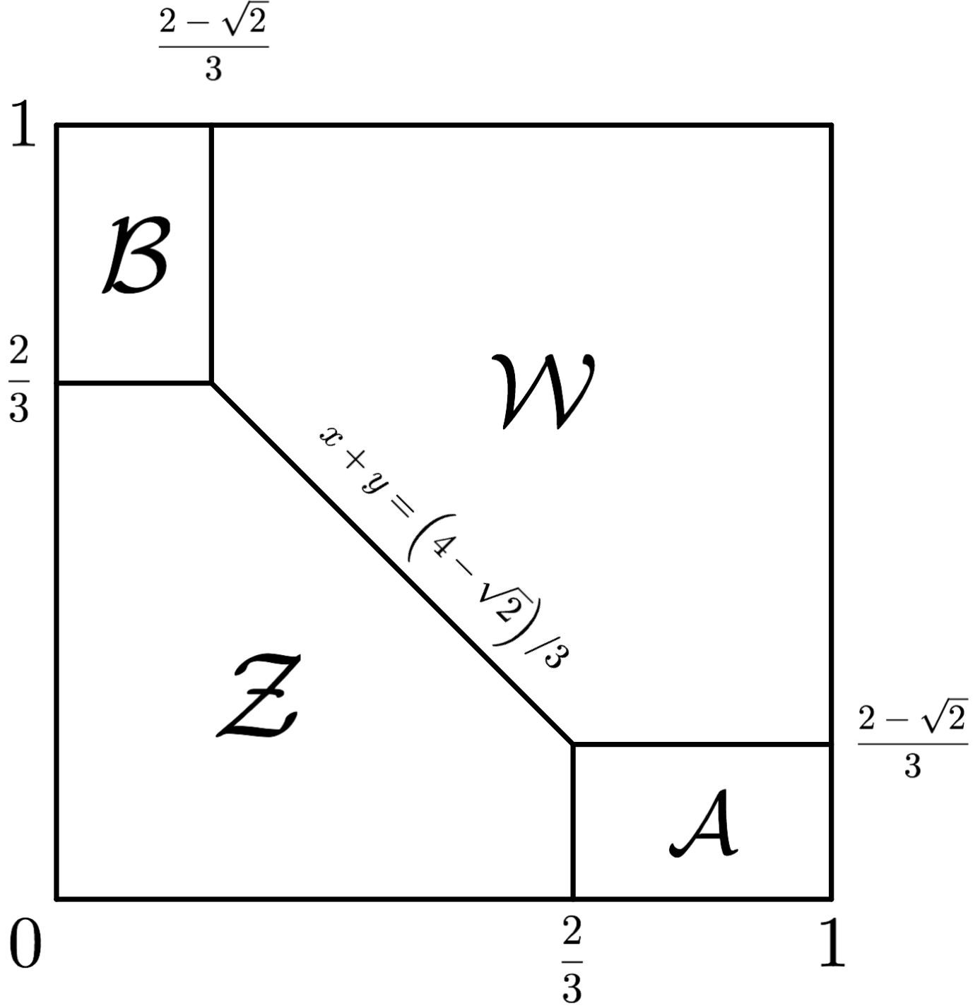
Refer to caption
Figure 4: Partition of the square with respect to the optimal uu.

The answers for the transform measure mm defined by (18) and for the optimal “imbalance” π=πopt\pi=\pi^{\mathrm{opt}} majorizing mm are as follows:

m=δ0+λ1|[0,1]×{0}+λ1|{0}×[0,1]−3​λ2|[0,1]2,m=\delta_{0}+\lambda_{1}|_{[0,1]\times\{0\}}+\lambda_{1}|_{\{0\}\times[0,1]}-3\lambda_{2}|_{[0,1]^{2}}, (84)
πopt=λ1|[0,1]×{0}+λ1|{0}×[0,1]−3​λ2|[0,1]2∖𝒵,\pi^{\mathrm{opt}}=\lambda_{1}|_{[0,1]\times\{0\}}+\lambda_{1}|_{\{0\}\times[0,1]}-3\lambda_{2}|_{[0,1]^{2}\setminus\mathcal{Z}}, (85)

where λ2,λ1\lambda_{2},\lambda_{1} are the two- and one-dimensional Lebesgue measures, respectively. We rely on these observations to simplify the construction.

Recall that for B=1B=1 bidder, the dual problem from Theorem 2 can be simplified (Corollary 3). It takes the following form:

minimize:∫[0,1]2(dς1+dς2)\mbox{minimize:}\quad\int_{[0,1]^{2}}\bigl(d\varsigma_{1}+d\varsigma_{2}\bigr) (86)

over vector measures ς=(ς1,ς2)\varsigma=(\varsigma_{1},\varsigma_{2}) satisfying

∫u​𝑑m≤∫(ux​d​ς1+uy​d​ς2)\int u{\,\mathrm{d}}m\leq\int(u_{x}d\varsigma_{1}+u_{y}d\varsigma_{2}) (87)

for all convex non-decreasing uu with u⁡(0)=0u(0)=0.

First, let us construct an absolutely continuous solution, i.e., such that d​ςi=ci​d​x​d​y{\,\mathrm{d}}\varsigma_{i}=c^{i}{\,\mathrm{d}}x{\,\mathrm{d}}y. We will need the following lemma.

Lemma 13.

Assume that a couple of nonnegative functions c1,c2c^{1},c^{2} satisfy

  1. 1.
    c1|𝒵∪ℬ=0,c2|𝒵∪𝒜=0,c^{1}|_{\mathcal{Z}\cup\mathcal{B}}=0,\ c^{2}|_{\mathcal{Z}\cup\mathcal{A}}=0, (88)
  2. 2.

    c1c^{1} is weakly differentiable along xx and satisfies the following integration by parts identity for every smooth φ\varphi

    ∫[0,1]2φx⋅c1dxdy=−∫[0,1]2φ⋅cx1dxdy+∫01φ(1,y)dy.\int_{[0,1]^{2}}\varphi_{x}\cdot c^{1}{\,\mathrm{d}}x{\,\mathrm{d}}y=-\int_{[0,1]^{2}}\varphi\cdot c^{1}_{x}{\,\mathrm{d}}x{\,\mathrm{d}}y+\int_{0}^{1}\varphi(1,y){\,\mathrm{d}}y.

    Similarly c2c^{2} is weakly differentiable along yy and satisfies the following integration by parts identity for every smooth φ\varphi

    ∫[0,1]2φy⋅c2dxdy=−∫[0,1]2φ⋅cy2dxdy+∫01φ(x,1)dx.\int_{[0,1]^{2}}\varphi_{y}\cdot c^{2}{\,\mathrm{d}}x{\,\mathrm{d}}y=-\int_{[0,1]^{2}}\varphi\cdot c^{2}_{y}{\,\mathrm{d}}x{\,\mathrm{d}}y+\int_{0}^{1}\varphi(x,1){\,\mathrm{d}}x.
  3. 3.
    cx1+cy2=3,c^{1}_{x}+c^{2}_{y}=3, (89)

    on [0,1]1∖𝒵[0,1]^{1}\setminus\mathcal{Z} almost everywhere.

Then the vector field c=(c1,c2)c=(c^{1},c^{2}) satisfies

div⁡[c]+πopt=0{\mathrm{div}}[c]+\pi^{\mathrm{opt}}=0 (90)

and ς=(ς1,ς2)\varsigma=(\varsigma_{1},\varsigma_{2}) such that d​ςi=ci​d​x​d​y{\,\mathrm{d}}\varsigma_{i}=c^{i}{\,\mathrm{d}}x{\,\mathrm{d}}y is a solution to the dual problem (86).

Proof.

Take any convex non-decreasing 11-Lipschitz function uu with u⁡(0)=0u(0)=0. Then

∫(x​ux+y​uy−u)​𝑑x​𝑑y=∫u​𝑑m≤∫u​d​πopt.\displaystyle\int\bigl(xu_{x}+yu_{y}-u\bigr){\,\mathrm{d}}x{\,\mathrm{d}}y=\int u{\,\mathrm{d}}m\leq\int u{\,\mathrm{d}}\pi^{\mathrm{opt}}.

The first equality is the definition of the transform measure mm, the second one holds since m⪯πoptm\preceq\pi^{\mathrm{opt}}. Since πopt\pi^{\mathrm{opt}} is given by an explicit formula (85), the identity for the divergence (90) follows from an elementary computation. Using (90) and the definition of divergence, we obtain

∫u​d​πopt\displaystyle\int u{\,\mathrm{d}}\pi^{\mathrm{opt}} =−∫udiv[c]dxdy=∫⟨∇u,c⟩dxdy≤\displaystyle=-\int u\ {\mathrm{div}}[c]{\,\mathrm{d}}x{\,\mathrm{d}}y=\int\langle\nabla u,c\rangle\ {\,\mathrm{d}}x{\,\mathrm{d}}y\leq
≤∫(c1+c2)​𝑑x​𝑑y=∫(d​ς1+d​ς2),\displaystyle\leq\int(c^{1}+c^{2}){\,\mathrm{d}}x{\,\mathrm{d}}y=\int\bigl(d\varsigma_{1}+d\varsigma_{2}\bigr),

where, we used that 0≤ux≤10\leq u_{x}\leq 1 and 0≤uy≤10\leq u_{y}\leq 1 to get the inequality. Substituting u=uoptu=u^{\mathrm{opt}} given by (83), we see that the two inequalities become equalities because u|𝒵=0u|_{\mathcal{Z}}=0 and c|𝒵=0c|_{\mathcal{Z}}=0. We conclude that the objective in the dual problem on ς\varsigma coincides with the optimal value of the primal problem ∫uopt​𝑑m\int u^{\mathrm{opt}}{\,\mathrm{d}}m. Thus ς\varsigma is the optimal solution of the dual. ∎

Example 1 (Absolutely continuous solution).

Consider the following vector field:

c⁡(x,y)=(c1​(x,y),c2​(x,y)),c(x,y)=(c^{1}(x,y),c^{2}(x,y)),

where

c2​(x,y)=c1​(y,x)c^{2}(x,y)=c^{1}(y,x)

and

c1​(x,y)={0(x,y)∈𝒵∪ℬ3​x−2(x,y)∈𝒜32​(x+y−4−23)(x,y)∈𝒲,x≤23,y≤2392​(1−x)​(y−2−23)+3​(x−23)(x,y)∈𝒲,23≤x≤1,2−23≤y≤2394​(x−2−23)2(x,y)∈𝒲,2−23≤x≤23,23≤y≤112+32​(x−23)(x,y)∈𝒲,23≤x≤1,23≤y≤1c^{1}(x,y)=\begin{cases}0&(x,y)\in\mathcal{Z}\cup\mathcal{B}\\ 3x-2&(x,y)\in\mathcal{A}\\ \frac{3}{2}\bigl(x+y-\frac{4-\sqrt{2}}{3}\bigr)&(x,y)\in\mathcal{W},x\leq\frac{2}{3},y\leq\frac{2}{3}\\ \frac{9}{2}(1-x)\bigl(y-\frac{2-\sqrt{2}}{3}\bigr)\\ \quad\quad\quad\quad+3(x-\frac{2}{3})&(x,y)\in\mathcal{W},\frac{2}{3}\leq x\leq 1,\frac{2-\sqrt{2}}{3}\leq y\leq\frac{2}{3}\\ \frac{9}{4}\bigl(x-\frac{2-\sqrt{2}}{3}\bigr)^{2}&(x,y)\in\mathcal{W},\frac{2-\sqrt{2}}{3}\leq x\leq\frac{2}{3},\frac{2}{3}\leq y\leq 1\\ \frac{1}{2}+\frac{3}{2}\bigl(x-\frac{2}{3}\bigr)&(x,y)\in\mathcal{W},\frac{2}{3}\leq x\leq 1,\frac{2}{3}\leq y\leq 1\end{cases}

One can check that the vector field c=(c1,c2)c=(c^{1},c^{2}) satisfies the assumptions of Lemma 13. We conclude that cc solves the dual problem.

Remark 2 (Non-uniqueness).

It turns out that there are many solutions to the dual problem. However, the reader should be not confused by existing results on uniqueness of the optimal vector field cc in Beckmann’s problem; see, e.g., Santambrogio 2015. Unlike most of the works on Beckmann’s problem, our cost function is given by the l1l^{1}-norm ∑i|ci|\sum_{i}|c_{i}| instead of the Euclidean l2l^{2}-norm ∑i|ci|2\sqrt{\sum_{i}|c_{i}|^{2}}. The l1l^{1}-norm constitutes a degenerate case. Indeed, if cc is a solution and φ\varphi is a smooth function, supported on a small neighbourhood of a point (x0,y0)∈int⁡(𝒲)(x_{0},y_{0})\in{\rm int}(\mathcal{W}), where ci​(x0,y0)>0c^{i}(x_{0},y_{0})>0, then for sufficiently small ε\varepsilon the vector field

cε=(c1+ε​φy,c2−ε​φx)c_{\varepsilon}=(c^{1}+\varepsilon\varphi_{y},c^{2}-\varepsilon\varphi_{x})

satisfies all the assumptions. Integrating by parts one gets

∫∑i=12cεi​𝑑x​𝑑y=∫∑i=12ci​𝑑x​𝑑y.\int\sum_{i=1}^{2}c^{i}_{\varepsilon}\ {\,\mathrm{d}}x{\,\mathrm{d}}y=\int\sum_{i=1}^{2}c^{i}\ {\,\mathrm{d}}x{\,\mathrm{d}}y.

Thus cεc_{\varepsilon} is also a solution.

Moreover, one can easily find solutions which are not weakly differentiable. Let a,δa,\delta be numbers and QQ be the square with the center (a,a)(a,a) and vertices

q−,a=(a−δ,a),qa,−=(a,a−δ),q+,a=(a+δ,a),qa,+=(a,a+δ).q_{-,a}=(a-\delta,a),\ \ q_{a,-}=(a,a-\delta),\ \ q_{+,a}=(a+\delta,a),\ \ q_{a,+}=(a,a+\delta).

Define

ψ1​(x,y)=IQ​(x,y)​(−Ia−δ≤x≤a​(x)+Ia≤x≤a+δ​(x))\psi_{1}(x,y)=I_{Q}(x,y)\bigl(-I_{a-\delta\leq x\leq a}(x)+I_{a\leq x\leq a+\delta}(x)\bigr)
ψ2​(x,y)=IQ​(x,y)​(−Ia−δ≤y≤a​(y)+Ia≤y≤a+δ​(y))\psi_{2}(x,y)=I_{Q}(x,y)\bigl(-I_{a-\delta\leq y\leq a}(y)+I_{a\leq y\leq a+\delta}(y)\bigr)

It is easy to verify that

∂ψ1​(x,y)∂y=∂ψ2​(x,y)∂x=12​[−λ1|[q−,a,qa,−]+λ1|[q−,a,qa,+]−λ1|[qa,+,q+,a]+λ1|[qa,−,q+,a]]\frac{\partial\psi_{1}(x,y)}{\partial y}=\frac{\partial\psi_{2}(x,y)}{\partial x}=\frac{1}{\sqrt{2}}\Bigl[-\lambda_{1}|_{[q_{-,a},q_{a,-}]}+\lambda_{1}|_{[q_{-,a},q_{a,+}]}-\lambda_{1}|_{[q_{a,+},q_{+,a}]}+\lambda_{1}|_{[q_{a,-},q_{+,a}]}\Bigr] (91)

in the weak sense, where [a,b][a,b] denotes the segment joining aa and bb. Clearly,

∫ψ1​𝑑x​𝑑y=∫ψ2​𝑑x​𝑑y=0\int\psi_{1}{\,\mathrm{d}}x{\,\mathrm{d}}y=\int\psi_{2}{\,\mathrm{d}}x{\,\mathrm{d}}y=0

and (91) implies that

div⁡[(ψ2,−ψ1)]=0.{\mathrm{div}}[(\psi_{2},-\psi_{1})]=0.

Thus for any solution cc to the dual problem, strictly positive in some neighbourhood UU of a point (a,a)∈int⁡(𝒲)(a,a)\in\rm{int}(\mathcal{W}), the vector field

c+(ψ2,−ψ1)c+(\psi_{2},-\psi_{1})

is a solution to the dual problem for sufficiently small δ\delta.

D.3.1 Singular solutions

It may seem intuitive — at least for our toy example — that vector fields solving the dual problem must be integrable functions. Surprisingly, there exist singular solutions. We construct a measure-valued solution ς\varsigma with the following properties:

  • •

    The vector field ς\varsigma is singular, i.e., its components are not absolutely continuous measures: namely, ς\varsigma has an atom at (1,1)(1,1).

  • •

    Because of this atom, the divergence of ς\varsigma is not a measure and can only be defined in the space of generalized functions.

Example 2 (Singular solution).

Define a couple of measures (ς1,ς2)(\varsigma_{1},\varsigma_{2}) as follows:

ς1\displaystyle\varsigma_{1} =𝟙​((x,y)∈𝒜)⋅3​(x−23)​d​x​d​y+\displaystyle=\mathbbm{1}((x,y)\in\mathcal{A})\cdot 3\left(x-\frac{2}{3}\right)\,{\,\mathrm{d}}x\,{\,\mathrm{d}}y+
+𝟙((x,y)∈𝒲∩{y≤23})⋅3(x+y−4−23)dxdy,\displaystyle\quad\quad+\mathbbm{1}\left((x,y)\in\mathcal{W}\cap\Bigl\{y\leq\frac{2}{3}\Bigr\}\right)\cdot 3\left(x+y-\frac{4-\sqrt{2}}{3}\right)\,{\,\mathrm{d}}x\,{\,\mathrm{d}}y,
ς2\displaystyle\varsigma_{2} =𝟙​(y≥23)⋅3​(y−23)​d​x​d​y+C⋅δ⁡(x=1,y=1),\displaystyle=\mathbbm{1}\left(y\geq\frac{2}{3}\right)\cdot 3\left(y-\frac{2}{3}\right)\,{\,\mathrm{d}}x\,{\,\mathrm{d}}y+C\cdot\delta(x=1,y=1),

where C=118+227C=\frac{1}{18}+\frac{\sqrt{2}}{27}; see Figure 4.

Let us show that the vector-measure ς=(ς1,ς2)\varsigma=(\varsigma_{1},\varsigma_{2}) is a solution to the dual problem. We need to demonstrate that ς\varsigma satisfies the majorization condition (87) and minimizes the dual objective (86) over such vector measures.

First, we check that ς\varsigma satisfies (87). Integrating by parts, we conclude that for any smooth uu defined on [0,1]2[0,1]^{2},

∫∂u∂x​d​ς1=∫02−23v⁡(y)​dy+∫2−2323v⁡(y)⋅3​(y+2−13)​dy−−3∫(𝒲∪𝒜)∩{y≤23}u(x,y)dxdy,∫∂u∂y​d​ς2=∫01u⁡(x,1)​dx+C⋅v′​(1)−3​∫y≥23u⁡(x,y)​dx​dy,\displaystyle\begin{split}\int\frac{\partial u}{\partial x}\,{\,\mathrm{d}}\varsigma_{1}&=\int_{0}^{\frac{2-\sqrt{2}}{3}}v(y)\,{\,\mathrm{d}}y+\int_{\frac{2-\sqrt{2}}{3}}^{\frac{2}{3}}v(y)\cdot 3\left(y+\frac{\sqrt{2}-1}{3}\right)\,{\,\mathrm{d}}y-\\ &\quad-3\int_{(\mathcal{W}\cup\mathcal{A})\cap\{y\leq\frac{2}{3}\}}u(x,y)\,{\,\mathrm{d}}x\,{\,\mathrm{d}}y,\\ \int\frac{\partial u}{\partial y}\,{\,\mathrm{d}}\varsigma_{2}&=\int_{0}^{1}u(x,1)\,{\,\mathrm{d}}x+C\cdot v^{\prime}(1)-3\int_{y\geq\frac{2}{3}}u(x,y)\,{\,\mathrm{d}}x\,{\,\mathrm{d}}y,\end{split} (92)

where v⁡(y)=u⁡(1,y)v(y)=u(1,y).

Let us prove that for any smooth convex non-decreasing uu with u⁡(0)=0u(0)=0,

∫01∫01(x⋅∂u∂x+y⋅∂u∂y−u)​𝑑x​𝑑y≤∫∂u∂x​d​ς1+∫∂u∂y​d​ς2.\displaystyle\int_{0}^{1}\int_{0}^{1}\left(x\cdot\frac{\partial u}{\partial x}+y\cdot\frac{\partial u}{\partial y}-u\right)\,{\,\mathrm{d}}x\,{\,\mathrm{d}}y\leq\int\frac{\partial u}{\partial x}\,{\,\mathrm{d}}\varsigma_{1}+\int\frac{\partial u}{\partial y}\,{\,\mathrm{d}}\varsigma_{2}.

Integrating by parts,

∫01∫01(x⋅∂u∂x+y⋅∂u∂y−u)​dx​dy==∫01u⁡(x,1)​dx+∫01v⁡(y)​dy−3​∫01∫01u⁡(x,y)​dx​dy.\int_{0}^{1}\int_{0}^{1}\left(x\cdot\frac{\partial u}{\partial x}+y\cdot\frac{\partial u}{\partial y}-u\right)\,{\,\mathrm{d}}x\,{\,\mathrm{d}}y=\\ =\int_{0}^{1}u(x,1)\,{\,\mathrm{d}}x+\int_{0}^{1}v(y)\,{\,\mathrm{d}}y-3\int_{0}^{1}\int_{0}^{1}u(x,y)\,{\,\mathrm{d}}x\,{\,\mathrm{d}}y.

Comparing it to (92), we conclude that the inequality above is equivalent to the following one:

C⋅v′(1)−∫231v(y)dy+∫2−2323v(y)⋅3(y−2−23)dy≥−3∫𝒵u(x,y)dxdy.C\cdot v^{\prime}(1)-\int_{\frac{2}{3}}^{1}v(y)\,{\,\mathrm{d}}y+\int_{\frac{2-\sqrt{2}}{3}}^{\frac{2}{3}}v(y)\cdot 3\left(y-\frac{2-\sqrt{2}}{3}\right)\,{\,\mathrm{d}}y\geq-3\int_{\mathcal{Z}}u(x,y)\,{\,\mathrm{d}}x\,{\,\mathrm{d}}y.

The right-hand side is non-positive, so it is sufficient to prove that the left-hand side is non-negative for any smooth convex non-decreasing uu with u⁡(0)=0u(0)=0. For any such uu, the function v⁡(y)=u⁡(1,y)v(y)=u(1,y) is a non-decreasing convex function defined on [0,1][0,1]. So, for any y∈[23,1]y\in\left[\frac{2}{3},1\right], we have v⁡(y)≤v⁡(2/3)+(y−2/3)⋅v′​(1)v(y)\leq v(2/3)+(y-2/3)\cdot v^{\prime}(1). Therefore,

∫231v⁡(y)​𝑑y≤13⋅v⁡(23)+118⋅v′​(1).\int_{\frac{2}{3}}^{1}v(y)\,{\,\mathrm{d}}y\leq\frac{1}{3}\cdot v\left(\frac{2}{3}\right)+\frac{1}{18}\cdot v^{\prime}(1).

In addition, for any y∈[2−23,23]y\in\left[\frac{2-\sqrt{2}}{3},\frac{2}{3}\right], we have

v⁡(23)−v⁡(y)≤v′​(23)⋅(23−y)≤v′​(1)⋅(23−y).v\left(\frac{2}{3}\right)-v(y)\leq v^{\prime}\left(\frac{2}{3}\right)\cdot\left(\frac{2}{3}-y\right)\leq v^{\prime}(1)\cdot\left(\frac{2}{3}-y\right).

Therefore,

∫2−2323v⁡(y)⋅3​(y−2−23)​dy≥≥v⁡(23)⋅∫2−23233​(y−2−23)​𝑑y−v′​(1)⋅∫2−23233​(y−2−23)​(23−y)​𝑑y=13⋅v⁡(23)−227⋅v′​(1).\int_{\frac{2-\sqrt{2}}{3}}^{\frac{2}{3}}v(y)\cdot 3\left(y-\frac{2-\sqrt{2}}{3}\right)\,{\,\mathrm{d}}y\geq\\ \geq v\left(\frac{2}{3}\right)\cdot\int_{\frac{2-\sqrt{2}}{3}}^{\frac{2}{3}}3\left(y-\frac{2-\sqrt{2}}{3}\right)\,{\,\mathrm{d}}y-v^{\prime}(1)\cdot\int_{\frac{2-\sqrt{2}}{3}}^{\frac{2}{3}}3\left(y-\frac{2-\sqrt{2}}{3}\right)\left(\frac{2}{3}-y\right)\,{\,\mathrm{d}}y\\ =\frac{1}{3}\cdot v\left(\frac{2}{3}\right)-\frac{\sqrt{2}}{27}\cdot v^{\prime}(1). (93)

Finally,

C⋅v′​(1)−∫231v⁡(y)​dy+∫2−2323v⁡(y)⋅3​(y−2−23)​dy≥≥C⋅v′​(1)−13⋅v⁡(23)−118⋅v′​(1)+13⋅v⁡(23)−227⋅v′​(1)=0.C\cdot v^{\prime}(1)-\int_{\frac{2}{3}}^{1}v(y)\,{\,\mathrm{d}}y+\int_{\frac{2-\sqrt{2}}{3}}^{\frac{2}{3}}v(y)\cdot 3\left(y-\frac{2-\sqrt{2}}{3}\right)\,{\,\mathrm{d}}y\geq\\ \geq C\cdot v^{\prime}(1)-\frac{1}{3}\cdot v\left(\frac{2}{3}\right)-\frac{1}{18}\cdot v^{\prime}(1)+\frac{1}{3}\cdot v\left(\frac{2}{3}\right)-\frac{\sqrt{2}}{27}\cdot v^{\prime}(1)=0. (94)

We conclude that (ς1,ς2)(\varsigma_{1},\varsigma_{2}) satisfies (87).

Let us verify the optimality of (ς1,ς2)(\varsigma_{1},\varsigma_{2}). It is enough to check that the value of the dual objective (86) on ς\varsigma coincides with the optimal value of the primal problem. Recall that uoptu^{\mathrm{opt}} denotes the optimal function in the primal problem. Hence,

∫(d​ς1+d​ς2)=∫∂uopt∂x​d​ς1+∫∂uopt∂y​d​ς2.\int\left({\,\mathrm{d}}\varsigma_{1}+{\,\mathrm{d}}\varsigma_{2}\right)=\int\frac{\partial u^{\mathrm{opt}}}{\partial x}\,{\,\mathrm{d}}\varsigma_{1}+\int\frac{\partial u^{\mathrm{opt}}}{\partial y}\,{\,\mathrm{d}}\varsigma_{2}.

Thus it is enough to check that the right-hand side is equal to the value of the primal problem:

∫01∫01(x⋅∂uopt∂x+y⋅∂uopt∂y−u)​𝑑x​𝑑y=∫∂uopt∂x​d​ς1+∫∂uopt∂y​d​ς2.\int_{0}^{1}\int_{0}^{1}\left(x\cdot\frac{\partial u^{\mathrm{opt}}}{\partial x}+y\cdot\frac{\partial u^{\mathrm{opt}}}{\partial y}-u\right)\,{\,\mathrm{d}}x\,{\,\mathrm{d}}y=\int\frac{\partial u^{\mathrm{opt}}}{\partial x}\,{\,\mathrm{d}}\varsigma_{1}+\int\frac{\partial u^{\mathrm{opt}}}{\partial y}\,{\,\mathrm{d}}\varsigma_{2}.

Equivalently,

C⋅(vopt)′​(1)−∫231vopt​(y)​dy+∫2−2323vopt​(y)⋅3​(y−2−23)​dy==−3∫𝒵uopt(x,y)dxdy.C\cdot(v^{\mathrm{opt}})^{\prime}(1)-\int_{\frac{2}{3}}^{1}v^{\mathrm{opt}}(y)\,{\,\mathrm{d}}y+\int_{\frac{2-\sqrt{2}}{3}}^{\frac{2}{3}}v^{\mathrm{opt}}(y)\cdot 3\left(y-\frac{2-\sqrt{2}}{3}\right)\,{\,\mathrm{d}}y=\\ =-3\int_{\mathcal{Z}}u^{\mathrm{opt}}(x,y)\,{\,\mathrm{d}}x\,{\,\mathrm{d}}y.

By (83), the right-hand side is equal to 0. The function voptv^{\mathrm{opt}} is linear on [2−23,1]\left[\frac{2-\sqrt{2}}{3},1\right] and, hence, both inequalities (93) and (94) hold as equalities. Therefore, the left-hand side is also 0. Thus ς\varsigma is an optimal solution to the dual problem as its objective (86) on ς\varsigma is equal to the optimal value of the primal problem.

D.4 Upper bound on auctioneer’s revenue

In Section 4, we showed that the auctioneer’s revenue is bounded from above by

B⋅inf(φi)i∈ℐ∑i∈ℐ(∫Xφi∗​(xi)​ρ​(x)​𝑑x+∫01φi​(zB−1)​𝑑z).B\cdot\inf_{\footnotesize{\begin{array}[]{c}(\varphi_{i})_{i\in\mathcal{I}}\end{array}}}\sum_{i\in\mathcal{I}}\left(\int_{X}\varphi_{i}^{*}(x_{i})\rho(x){\,\mathrm{d}}x+\int_{0}^{1}\varphi_{i}\left(z^{B-1}\right){\,\mathrm{d}}z\right). (95)

for any number BB of bidders, II of items, and any density ρ\rho; see formula (22). Here we show that this upper bound corresponds to full surplus extraction.

Our goal is to show that the expression (95) equals to the full surplus defined by

∑y∈ℐ𝔼⁡[maxb∈ℬ⁡χb,i],\sum_{y\in\mathcal{I}}\mathbb{E}\left[\max_{b\in\mathcal{B}}\chi_{b,i}\right], (96)

where χb∈X\chi_{b}\in X are i.i.d. random vectors distributed with density ρ\rho.

Let ρi\rho_{i} be the one-dimensional marginals of ρ\rho onto the ii-th coordinate. Then (95) equals to B​∑i∈ℐD​M​KiB\sum_{i\in\mathcal{I}}DMK_{i}, where

D​M​Ki=inf(φi)i∈ℐ(∫01φi∗​(xi)​ρi​(xi)​d​xi+1B−1​∫01φi​(yi)​yi2−BB−1​d​yi).DMK_{i}=\inf_{\footnotesize{\begin{array}[]{c}(\varphi_{i})_{i\in\mathcal{I}}\end{array}}}\left(\int_{0}^{1}\varphi_{i}^{*}(x_{i})\rho_{i}(x_{i}){\,\mathrm{d}}x_{i}+\frac{1}{B-1}\int_{0}^{1}\varphi_{i}(y_{i})y^{\frac{2-B}{B-1}}_{i}{\,\mathrm{d}}y_{i}\right).

The value D​M​KiDMK_{i} is nothing else but the value of the dual Monge–Kantorovich problem for the cost function −xi​yi-x_{i}y_{i}. Adding the terms 12​∫01xi2​ρi​(xi)​d​xi\frac{1}{2}\int_{0}^{1}x^{2}_{i}\rho_{i}(x_{i}){\,\mathrm{d}}x_{i} and 12​(B−1)​∫01yi2+2−BB−1​d​yi\frac{1}{2(B-1)}\int_{0}^{1}y^{2+\frac{2-B}{B-1}}_{i}{\,\mathrm{d}}y_{i} with known value, the reader can easily verify that this problem is equivalent to the transportation problem with the standard cost 12​|xi−yi|2\frac{1}{2}|x_{i}-y_{i}|^{2}. Thus, according to the one-dimensional version of the Brenier theorem, the solution is concentrated on the graph of the mapping TiT_{i} given by

∫0tiρi​d​xi=1B−1​∫0T⁡(ti)yi2−BB−1​d​yi=Ti1B−1​(ti)\int_{0}^{t_{i}}\rho_{i}{\,\mathrm{d}}x_{i}=\frac{1}{B-1}\int_{0}^{T(t_{i})}y_{i}^{\frac{2-B}{B-1}}{\,\mathrm{d}}y_{i}=T^{\frac{1}{B-1}}_{i}(t_{i})

and the cost equals ∫01xi​Ti​(xi)​ρi​d​xi\int_{0}^{1}x_{i}T_{i}(x_{i})\rho_{i}{\,\mathrm{d}}x_{i}. Let FiF_{i} be the cumulative distribution function of xix_{i}. Finally, we get

D​M​Ki=∫01xi​FiB−1​(xi)​ρi​(xi)​d​xi=1B​∫01xi​ρi​(xi)​d​FiB​(xi)=1B​𝔼​[maxb∈ℬ⁡χb,i]DMK_{i}=\int_{0}^{1}x_{i}F_{i}^{B-1}(x_{i})\rho_{i}(x_{i}){\,\mathrm{d}}x_{i}=\frac{1}{B}\int_{0}^{1}x_{i}\rho_{i}(x_{i}){\,\mathrm{d}}F_{i}^{B}(x_{i})=\frac{1}{B}\mathbb{E}\left[\max_{b\in\mathcal{B}}\chi_{b,i}\right]

and conclude that (95) is equal to (96).

Appendix E Numerical approach

This section is devoted to computing the auctioneer’s optimal revenue and an optimal reduced-form mechanism. By Proposition 1, the auctioneer’s problem is equivalent to the multi-bidder Rochet-Choné problem (11). We describe a numerical approximation scheme for this problem and prove convergence results.

Recall that in the multi-bidder Rochet-Choné problem, we are given the number BB of bidders, the set ℐ\mathcal{I} of |ℐ|=I|\mathcal{I}|=I items, and a distribution μ\mu on the set of types X=[0,1]ℐX=[0,1]^{\mathcal{I}} with density ρ\rho. Let η\eta be the majorizing measure equal to the distribution of ξB−1\xi^{B-1}, where ξ\xi is uniform on [0,1][0,1]. The goal is to maximize

B⋅∫X(⟨∇u​(x),x⟩−u⁡(x))​𝑑μ​(x)B\cdot\int_{X}\Big(\langle\nabla u(x),x\rangle-u(x)\Big){\,\mathrm{d}}\mu(x)

over functions u∈𝒰Lip,1u\in\mathcal{U}_{{\mathrm{Lip}},1} satisfying the majorization constraint

law⁡(uxi)⪯η,\mathrm{law}(u_{x_{i}})\preceq\eta,

for all i∈ℐi\in\mathcal{I}. Recall that 𝒰Lip,1\mathcal{U}_{{\mathrm{Lip}},1} is the set of 11-Lipshitz convex non-decreasing functions u:X→ℝ+u:\ X\to\mathbb{R}_{+}, law⁡(ξ)\mathrm{law}(\xi) denotes the distribution of a random variable ξ\xi, and the partial derivative uxi=uxi​(χ)u_{x_{i}}=u_{x_{i}}(\chi) is treated as a random variable assuming that its argument χ\chi is distributed according to μ\mu.

We will assume that the distribution μ\mu satisfies the following assumption:

Assumption 1.

The density ρ\rho is a continuously differentiable function, and there exist constants 0<c<C0<c<C such that c≤ρ⁡(x)≤Cc\leq\rho(x)\leq C for all x∈Xx\in{X}.

Outline of the results.

The multi-bidder Rochet-Choné problem is a well-defined optimization problem, however, converting it into an algorithm approximating the solution — a numerical approximation scheme — is not straightforward. The first obstacle is that the solution uu as well as the input data μ\mu and η\eta are continuous objects. Hence, the problem is to be discretized in a way that solutions of the discrete problems approximate those of the continuous one. The second obstacle is that the majorization constraint, in addition to requiring discretization, is non-linear.

We demonstrate that the majorization constraint is equivalent to a linear constraint suggested by a connection between majorization and martingales and construct provably convergent approximations. As a result, we obtain a finite-dimensional linear program approximating the original Rochet-Choné problem. To summarize, the approach consists of three steps:

  1. 1.

    discretize the set of types X=[0,1]ℐX=[0,1]^{\mathcal{I}} and the distribution μ\mu;

  2. 2.

    approximate the gradient ∇u\nabla u and the convexity constraint u∈𝒰Lip,1u\in\mathcal{U}_{{\mathrm{Lip}},1};

  3. 3.

    linearize and approximate the majorization constraint law⁡(uxi)⪯η\mathrm{law}(u_{x_{i}})\preceq\eta;

  4. 4.

    use an LP solver to find a solution to the resulting linear program.

Section E.1 describes the second step, the third step is discussed in Section E.2, and Section E.3 contains provable heuristics improving the run time. Here we provide a high-level overview.

To discretize the domain X=[0,1]ℐ{X}=[0,1]^{\mathcal{I}}, we consider the uniform partition of XX into nIn^{I} equal cubes and replace the probability distribution μ\mu with the associated sum of point masses. After that, we approximate the initial auction design problem with the corresponding discrete version. The convexity constraint can be written as follows:

u⁡(θi)−u⁡(θj)≥⟨∇u​(θj),θi−θj⟩for all θi, θj from the discrete lattice.u(\theta_{i})-u(\theta_{j})\geq\langle\nabla u(\theta_{j}),\theta_{i}-\theta_{j}\rangle\quad\text{for all $\theta_{i}$, $\theta_{j}$ from the discrete lattice.} (97)

This approach is based on the algorithm described by Ekeland and Moreno-Bromberg 2010. To approximate the majorization constraint, we use a generalization of Strassen’s theorem Strassen 1965 reducing the constraint to the existence of the supermartingale with the given marginals. To get a finite-dimensional linear program, we discretize the distribution η\eta. The convergence of the discretization is demonstrated in Theorem 7, Theorem 9, and Corollary 8.

In practice, the computation can be sped up by reducing the size of the linear program, which can be achieved via heuristics identifying redundant constraints. The approach of “directional convexity” by Oberman 2013 allows us to reduce the number of convexity constraints in (97) and results in the substantial improvement in computation time.

For simplicity, we focus on the case of a common majorizing measure η=law⁡(ξB−1)\eta=\mathrm{law}(\xi^{B-1}) with ξ∼Uniform⁡[0,1]\xi\sim\mathrm{Uniform}[0,1]. The results can be easily extended to the Rochet-Choné problem with general majorization (49) and distinct majorizing measures ηi\eta_{i}.

E.1 Convexity constraint approximation

With the continuous problem, we associate its discrete version as described in (Ekeland and Moreno-Bromberg 2010, Section 3).

Fix a positive integer nn. We partition the domain X=[0,1]ℐX=[0,1]^{\mathcal{I}} into nIn^{I} equal cubes with the edge length 1/n1/n. The elements of the partition will be denoted by σj(n)\sigma_{j}^{(n)}, 1≤j≤nI1\leq j\leq n^{I}. Denote

Θn={θj(n):1≤j≤nI},\Theta_{n}=\{\theta_{j}^{(n)}\colon 1\leq j\leq n^{I}\},

where θj(n)\theta_{j}^{(n)} is the center of the cube σj(n)\sigma_{j}^{(n)}. Finally, we denote

μj(n)=1nI⋅min⁡{ρ⁡(x):x∈σj(n)}.\mu_{j}^{(n)}=\frac{1}{n^{I}}\cdot\min\{\rho(x)\colon x\in\sigma_{j}^{(n)}\}.

Note that the weight sum ∑jμk(n)\sum_{j}\mu_{k}^{(n)} is not necessary equal to 1; therefore, we define μ0(n)=1−∑j=1nIμj(n)\mu_{0}^{(n)}=1-\sum_{j=1}^{n^{I}}\mu_{j}^{(n)}.

For every 1≤j≤nI1\leq j\leq n^{I}, we associate with the cube σj(n)\sigma_{j}^{(n)} the scalar variable uj(n)u_{j}^{(n)} that corresponds to the value of the utility function uu at θj(n)\theta_{j}^{(n)}, and the vector variable pj(n)=(pj,1(n),…,pj,I(n))∈ℝℐp_{j}^{(n)}=(p_{j,1}^{(n)},\dots,p_{j,{I}}^{(n)})\in\mathbb{R}^{\mathcal{I}} that corresponds to the value of ∇u\nabla u at θj(n)\theta_{j}^{(n)}. After that, we define the following non-linear program 𝒟n\mathcal{D}_{n}:

maximize:∑jμj(n)⋅(⟨θj(n),pj(n)⟩−uj(n))\displaystyle\text{maximize:}\quad\sum_{j}\mu_{j}^{(n)}\cdot\left(\langle\theta_{j}^{(n)},p_{j}^{(n)}\rangle-u_{j}^{(n)}\right) (𝒟n\mathcal{D}_{n})
subject to:
(ir)uj(n)≥0\displaystyle\quad\text{{(ir)}}\quad u_{j}^{(n)}\geq 0\quad for all ​1≤j≤nI;\displaystyle\text{for all }1\leq j\leq n^{I};
(fs)0≤pj,k(n)≤1\displaystyle\quad\text{{(fs)}}\quad 0\leq p_{j,k}^{(n)}\leq 1\quad for all ​1≤j≤nI,k∈ℐ;\displaystyle\text{for all }1\leq j\leq n^{I},k\in\mathcal{I};
(ic)ui(n)−uj(n)≥⟨θi(n)−θj(n),pj(n)⟩\displaystyle\quad\text{{(ic)}}\quad u_{i}^{(n)}-u_{j}^{(n)}\geq\langle\theta_{i}^{(n)}-\theta_{j}^{(n)},p_{j}^{(n)}\rangle\quad for all ​1≤i,j≤nI;\displaystyle\text{for all }1\leq i,j\leq n^{I};
(mj)μ0(n)⋅δ⁡(x=0)+∑jμj(n)⋅δ⁡(x=pj,k(n))⪯η\displaystyle\quad\text{{(mj)}}\quad\mu_{0}^{(n)}\cdot\delta(x=0)+\sum_{j}\mu_{j}^{(n)}\cdot\delta\left(x=p_{j,k}^{(n)}\right)\preceq\eta\quad for all ​k∈ℐ.\displaystyle\text{for all }k\in\mathcal{I}.

Here, the shortcuts (ir), (fs), (ic), and (mj) correspond to the individual rationality, feasibility, incentive compatibility, and majorization, respectively. The only non-linear constraint in this program is (mj) discussed in the next section.

Given a solution (u¯(n),p¯(n))(\overline{u}^{(n)},\overline{p}^{(n)}), we define a function

u¯(n)​(x)=max⁡{0,maxj⁡{uj(n)+⟨x−θj(n),pj(n)⟩}}.\overline{u}^{(n)}(x)=\max\left\{0,\,\max_{j}\left\{u_{j}^{(n)}+\langle x-\theta_{j}^{(n)},p_{j}^{(n)}\rangle\right\}\right\}.

One can easily check that u¯(n)∈𝒰Lip,1\overline{u}^{(n)}\in\mathcal{U}_{{\mathrm{Lip}},1}, u¯(n)​(θj(n))=u¯j(n)\overline{u}^{(n)}\big(\theta_{j}^{(n)}\big)=\overline{u}^{(n)}_{j}, and p¯j(n)∈∂u¯(n)​(θj(n))\overline{p}_{j}^{(n)}\in\partial\overline{u}^{(n)}\big(\theta_{j}^{(n)}\big) for all 1≤j≤nI1\leq j\leq n^{I}. Unfortunately, it does not necessary true that law⁡(u¯xi(n))⪯η\mathrm{law}(\overline{u}^{(n)}_{x_{i}})\preceq\eta; therefore, the function u¯(n)\overline{u}^{(n)} does not necessary correspond to the interim utility function of a feasible auction mechanism. Nevertheless, we prove that the limiting function u¯\overline{u} satisfies the majorization constraint:

Proposition 11.

There exists a subsequence {u¯nk}⊂{u¯n}\{\overline{u}_{n_{k}}\}\subset\{\overline{u}_{n}\} such that:

  1. (a)

    the subsequence {u¯nk}\{\overline{u}_{n_{k}}\} converges uniformly to u¯\overline{u};

  2. (b)

    the function u¯∈𝒰Lip,1\overline{u}\in\mathcal{U}_{{\mathrm{Lip}},1} and law⁡(u¯xi)⪯η\mathrm{law}(\overline{u}_{x_{i}})\preceq\eta for all i∈ℐi\in\mathcal{I};

  3. (c)

    limk→∞∑jμj(n)⋅(⟨θj(nk),p¯j(nk)⟩−u¯j(nk))=∫X(⟨x,∇u¯​(x)⟩−u¯​(x))​𝑑μ\displaystyle\lim_{k\to\infty}\sum_{j}\mu_{j}^{(n)}\cdot\left(\langle\theta_{j}^{(n_{k})},\overline{p}_{j}^{(n_{k})}\rangle-\overline{u}_{j}^{(n_{k})}\right)=\int_{{X}}\left(\langle x,\nabla\overline{u}(x)\rangle-\overline{u}(x)\right)\,{\,\mathrm{d}}\mu

Before proving Proposition 11, we need the following technical result:

Lemma 14.

Let QQ be a compact subset of ℝℐ\mathbb{R}^{\mathcal{I}}. Consider a function ϕ⁡(θ,z,p)∈C1​(X×ℝ×Q→ℝ)\phi(\theta,z,p)\in C^{1}({X}\times\mathbb{R}\times Q\to\mathbb{R}). Let fk:X→ℝf_{k}\colon{X}\to\mathbb{R} be a family of convex functions such that ∂fk​(θ)∈Q\partial f_{k}(\theta)\in Q for all θ∈X\theta\in{X}, whose uniform limit is ff. Then

limk→∞∑jμj(n)⋅ϕ⁡(θj(n),fn​(θj(n)),∇fn​(θj(n)))=∫Xϕ⁡(θ,f⁡(θ),∇f​(θ))​𝑑μ.\lim_{k\to\infty}\sum_{j}\mu_{j}^{(n)}\cdot\phi\left(\theta_{j}^{(n)},f_{n}(\theta_{j}^{(n)}),\nabla f_{n}(\theta_{j}^{(n)})\right)=\int_{{X}}\phi(\theta,f(\theta),\nabla f(\theta))\,{\,\mathrm{d}}\mu.
Proof of Lemma 14.

The proof is based on the following result.

Lemma (Ekeland and Moreno-Bromberg 2010, Lemma A.6).

Under the assumptions of Lemma 14, for every ε>0\varepsilon>0 there exists K∈ℕK\in\mathbb{N} such that

|1nI​∑jϕ⁡(θj(n),fn​(θj(n)),∇fn​(θj(n)))−∫Xϕ⁡(θ,fn​(θ),∇fn​(θ))​𝑑θ|<ε\left|\frac{1}{n^{I}}\sum_{j}\phi\left(\theta_{j}^{(n)},f_{n}(\theta_{j}^{(n)}),\nabla f_{n}(\theta_{j}^{(n)})\right)-\int_{{X}}\phi(\theta,f_{n}(\theta),\nabla f_{n}(\theta))\,{\,\mathrm{d}}\theta\right|<\varepsilon

for all n>Kn>K.

Consider a function ψ⁡(θ,z,p)=ρ⁡(θ)⋅ϕ⁡(θ,z,p)\psi(\theta,z,p)=\rho(\theta)\cdot\phi(\theta,z,p), where ρ\rho is the density of μ\mu. The function ψ\psi is continuously differentiable; therefore, for every ε>0\varepsilon>0 there exists K∈ℕK\in\mathbb{N} such that

|1nI​∑jψ⁡(θj(n),fn​(θj(n)),∇fn​(θj(n)))−∫Xψ⁡(θ,fn​(θ),∇fn​(θ))​dθ|==|1nI​∑jρ⁡(θj(n))⋅ϕ⁡(θj(n),fn​(θj(n)),∇fn​(θj(n)))−∫Xϕ⁡(θ,fn​(θ),∇fn​(θ))​𝑑μ|<ε\displaystyle\begin{split}&\left|\frac{1}{n^{I}}\sum_{j}\psi\left(\theta_{j}^{(n)},f_{n}(\theta_{j}^{(n)}),\nabla f_{n}(\theta_{j}^{(n)})\right)-\int_{{X}}\psi(\theta,f_{n}(\theta),\nabla f_{n}(\theta))\,{\,\mathrm{d}}\theta\right|=\\ &=\left|\frac{1}{n^{I}}\sum_{j}\rho(\theta_{j}^{(n)})\cdot\phi\left(\theta_{j}^{(n)},f_{n}(\theta_{j}^{(n)}),\nabla f_{n}(\theta_{j}^{(n)})\right)-\int_{{X}}\phi(\theta,f_{n}(\theta),\nabla f_{n}(\theta))\,{\,\mathrm{d}}\mu\right|<\varepsilon\end{split} (98)

for all n>Kn>K.

Since all fnf_{n} are convex and {fn}\{f_{n}\} converges uniformly to ff, the sequence of gradients {∇fn​(θ)}\{\nabla f_{n}(\theta)\} converges to ∇f​(θ)\nabla f(\theta) for almost all θ∈X\theta\in{X}. Thus it follows from the continuity of ϕ\phi that

limn→∞ϕ⁡(θ,fn​(θ),∇fn​(θ))=ϕ⁡(θ,f⁡(θ),∇f​(θ))\lim_{n\to\infty}\phi(\theta,f_{n}(\theta),\nabla f_{n}(\theta))=\phi(\theta,f(\theta),\nabla f(\theta))

for almost all θ∈X\theta\in{X}. We may assume that the family of functions fnf_{n} is uniformly bounded. Therefore, there exists a constant MM such that

|ϕ⁡(θ,fn​(θ),∇fn​(θ))|<M\left|\phi(\theta,f_{n}(\theta),\nabla f_{n}(\theta))\right|<M

for all θ∈X\theta\in{X} and for all nn. Thus it follows from Lebesgue’s dominated convergence theorem that

limn→∞∫Xϕ⁡(θ,fn​(θ),∇fn​(θ))​𝑑μ=∫Xϕ⁡(θ,f⁡(θ),∇f​(θ))​𝑑μ.\lim_{n\to\infty}\int_{{X}}\phi(\theta,f_{n}(\theta),\nabla f_{n}(\theta))\,{\,\mathrm{d}}\mu=\int_{{X}}\phi(\theta,f(\theta),\nabla f(\theta))\,{\,\mathrm{d}}\mu. (99)

Finally, we have

|1nI∑jρ(θj(n))⋅ϕ(θj(n),fn(θj(n)),∇fn(θj(n)))−−∑jμj(n)⋅ϕ(θj(n),fn(θj(n)),∇fn(θj(n)))|≤≤M⋅∑j|ρ⁡(θj(n))nI−μj(n)|≤M⋅supj;x,y∈σj(n)|ρ⁡(x)−ρ⁡(y)|,\displaystyle\begin{split}&\Bigg|\frac{1}{n^{I}}\sum_{j}\rho(\theta_{j}^{(n)})\cdot\phi\left(\theta_{j}^{(n)},f_{n}(\theta_{j}^{(n)}),\nabla f_{n}(\theta_{j}^{(n)})\right)-\\ &\quad\quad\quad\quad-\sum_{j}\mu_{j}^{(n)}\cdot\phi\left(\theta_{j}^{(n)},f_{n}(\theta_{j}^{(n)}),\nabla f_{n}(\theta_{j}^{(n)})\right)\Bigg|\leq\\ &\quad\leq M\cdot\sum_{j}\left|\frac{\rho(\theta_{j}^{(n)})}{n^{I}}-\mu_{j}^{(n)}\right|\leq M\cdot\sup_{j;\,\,x,y\in\sigma_{j}^{(n)}}|\rho(x)-\rho(y)|,\end{split} (100)

and the latter expression tends to 0 as n→∞n\to\infty by the uniform continuity of ρ\rho.

Combining the expressions (98), (99) and (100), we obtain the desired convergence equality. ∎

Proof of Proposition 11.

Since u¯(n)∈𝒰Lip,1\overline{u}^{(n)}\in\mathcal{U}_{{\mathrm{Lip}},1} and this set space is sequentially compact in the uniform convergence topology (Lemma 5), there is a subsequence {u¯nk}\{\overline{u}_{n_{k}}\} that converges uniformly to the function u¯∈𝒰Lip,1\overline{u}\in\mathcal{U}_{{\mathrm{Lip}},1}.

To prove the majorization condition, it is sufficient to check that for any continuously differentiable non-decreasing convex function φ\varphi, we have

∫φ⁡(u¯xi)​𝑑μ≤∫01φ⁡(x)​𝑑η​(x).\int\varphi(\overline{u}_{x_{i}})\,{\,\mathrm{d}}\mu\leq\int_{0}^{1}\varphi(x)\,{\,\mathrm{d}}\eta(x). (101)

It follows from Lemma 14 that

|∫φ⁡(u¯xi)​𝑑μ−∑jμj(nk)⋅φ⁡(p¯j,i(nk))|≤ε⁡(k)\left|\int\varphi(\overline{u}_{x_{i}})\,{\,\mathrm{d}}\mu-\sum_{j}\mu_{j}^{(n_{k})}\cdot\varphi\big(\overline{p}_{j,i}^{(n_{k})}\big)\right|\leq\varepsilon(k)

and ε⁡(k)→0\varepsilon(k)\to 0 as k→+∞k\to+\infty. It follows from the (mj) constraint that

∑jμj(nk)⋅φ⁡(p¯j,i(nk))≤∫01φ⁡(x)​𝑑η​(x);\sum_{j}\mu_{j}^{(n_{k})}\cdot\varphi\big(\overline{p}_{j,i}^{(n_{k})}\big)\leq\int_{0}^{1}\varphi(x)\,{\,\mathrm{d}}\eta(x);

therefore, letting kk tend to +∞+\infty, we conclude that the inequality (101) holds. The point (c) also follows directly from Lemma 14. ∎

Let uopt∈𝒰Lip,1u^{\mathrm{opt}}\in\mathcal{U}_{{\mathrm{Lip}},1} be the optimum of the multi-bidder Rochet-Choné problem. For each positive integer nn, denote

ujopt,(n)=nI⋅∫σj(n)uopt​(x)​𝑑x,\displaystyle u_{j}^{\mathrm{opt},(n)}=n^{I}\cdot\int_{\sigma_{j}^{(n)}}u^{\mathrm{opt}}(x)\,{\,\mathrm{d}}x,
pj,kopt,(n)=nI⋅∫σj(n)uxkopt​(x)​𝑑x.\displaystyle p_{j,k}^{\mathrm{opt},(n)}=n^{I}\cdot\int_{\sigma_{j}^{(n)}}u^{\mathrm{opt}}_{x_{k}}(x)\,{\,\mathrm{d}}x.
Proposition 12.

The variables ujopt,(n)u_{j}^{\mathrm{opt},(n)} and pjopt,(n)p_{j}^{\mathrm{opt},(n)} satisfy all the constraints of the program 𝒟n\mathcal{D}_{n}.

Proof.

The constraints (ir) and (fs) follow from the inequalities uopt​(x)≥0u^{\mathrm{opt}}(x)\geq 0 and 0≤uxkopt​(x)≤10\leq u^{\mathrm{opt}}_{x_{k}}(x)\leq 1.

Since uopt​(x)u^{\mathrm{opt}}(x) is convex, we have

uopt​(x−θj(n)+θi(n))−uopt​(x)≥⟨θi(n)−θj(n),∇uopt​(x)⟩u^{\mathrm{opt}}\big(x-\theta_{j}^{(n)}+\theta_{i}^{(n)}\big)-u^{\mathrm{opt}}(x)\geq\langle\theta_{i}^{(n)}-\theta_{j}^{(n)},\nabla u^{\mathrm{opt}}(x)\rangle

for almost all x∈σj(n)x\in\sigma_{j}^{(n)}. Integrating this inequality over the cube σj(n)\sigma_{j}^{(n)}, we conclude that

uiopt,(n)−ujopt,(n)≥⟨θi(n)−θj(n),pjopt,(n)⟩.u_{i}^{\mathrm{opt},(n)}-u_{j}^{\mathrm{opt},(n)}\geq\langle\theta_{i}^{(n)}-\theta_{j}^{(n)},p_{j}^{\mathrm{opt},(n)}\rangle.

Thus the constraint (ic) holds.

Consider any non-decreasing convex function function φ\varphi. Since law⁡(uxiopt)⪯ηi\mathrm{law}(u_{x_{i}}^{\mathrm{opt}})\preceq\eta_{i}, we conclude that

∫01φ⁡(x)​𝑑η​(x)≥∑j∫σj(n)φ⁡(uxiopt)​𝑑μ.\int_{0}^{1}\varphi(x)\,{\,\mathrm{d}}\eta(x)\geq\sum_{j}\int_{\sigma_{j}^{(n)}}\varphi(u_{x_{i}}^{\mathrm{opt}})\,{\,\mathrm{d}}\mu.

Since φ⁡(x)\varphi(x) is non-decreasing, we have

∫σj(n)φ⁡(uxiopt)​𝑑μ≥μj(n)⋅nI⋅∫σj(n)φ⁡(uxiopt)​𝑑x+(μ⁡(σj(n))−μj(n))⋅φ⁡(0).\int_{\sigma_{j}^{(n)}}\varphi(u_{x_{i}}^{\mathrm{opt}})\,{\,\mathrm{d}}\mu\geq\mu_{j}^{(n)}\cdot n^{I}\cdot\int_{\sigma_{j}^{(n)}}\varphi(u_{x_{i}}^{\mathrm{opt}})\,{\,\mathrm{d}}x+\left(\mu(\sigma_{j}^{(n)})-\mu_{j}^{(n)}\right)\cdot\varphi(0).

Finally, it follows from Jensen’s inequality that

nI⋅∫σj(n)φ⁡(uxiopt)​𝑑x≥φ⁡(nI⋅∫σj(n)uxiopt​(x)​𝑑x)=φ⁡(pj,iopt,(n))n^{I}\cdot\int_{\sigma_{j}^{(n)}}\varphi(u_{x_{i}}^{\mathrm{opt}})\,{\,\mathrm{d}}x\geq\varphi\left(n^{I}\cdot\int_{\sigma_{j}^{(n)}}u_{x_{i}}^{\mathrm{opt}}(x)\,{\,\mathrm{d}}x\right)=\varphi\big(p_{j,i}^{\mathrm{opt},(n)}\big)

Thus

∫01φ⁡(x)​𝑑η​(x)≥∑jμj(n)⋅φ⁡(pj,iopt,(n))+μ0(n)⋅φ⁡(0).\int_{0}^{1}\varphi(x)\,{\,\mathrm{d}}\eta(x)\geq\sum_{j}\mu_{j}^{(n)}\cdot\varphi\big({p}_{j,i}^{\mathrm{opt},(n)}\big)+\mu_{0}^{(n)}\cdot\varphi(0).

Since this inequality holds for all φ\varphi, we conclude that the constraint (mj) holds. ∎

The next result demonstrates that the optimal revenue in the continuous problem is approximated by its discretization.

Proposition 13.

The following identity holds:

limn→∞∑jμj(n)⋅(⟨θj(n),pjopt,(n)⟩−ujopt,(n))=∫X(⟨x,∇uopt​(x)⟩−uopt​(x))​𝑑μ.\lim_{n\to\infty}\sum_{j}\mu_{j}^{(n)}\cdot\left(\langle\theta_{j}^{(n)},p_{j}^{\mathrm{opt},(n)}\rangle-u_{j}^{\mathrm{opt},(n)}\right)=\int_{{X}}\left(\langle x,\nabla u^{\mathrm{opt}}(x)\rangle-u^{\mathrm{opt}}(x)\right)\,{\,\mathrm{d}}\mu.
Proof.

The definition of ujopt,(n)u_{j}^{\mathrm{opt},(n)} and pjopt,(n)p_{j}^{\mathrm{opt},(n)} implies that

∫X(⟨x,∇uopt​(x)⟩−uopt​(x))​dμ−∑jμj(n)⋅(⟨θj(n),pjopt,(n)⟩−ujopt,(n))==∑j∫σj(n)(⟨x,∇uopt​(x)⟩−uopt​(x))⋅(ρ⁡(x)−nI​μj(n))​dx≤≤supx∈X|⟨x,∇uopt​(x)⟩−uopt​(x)|⋅supj,x∈σj(n)|ρ⁡(x)−nI​μj(n)|.\int_{{X}}\left(\langle x,\nabla u^{\mathrm{opt}}(x)\rangle-u^{\mathrm{opt}}(x)\right)\,{\,\mathrm{d}}\mu-\sum_{j}\mu_{j}^{(n)}\cdot\left(\langle\theta_{j}^{(n)},p_{j}^{\mathrm{opt},(n)}\rangle-u_{j}^{\mathrm{opt},(n)}\right)=\\ =\sum_{j}\int_{\sigma_{j}^{(n)}}\left(\langle x,\nabla u^{\mathrm{opt}}(x)\rangle-u^{\mathrm{opt}}(x)\right)\cdot\left(\rho(x)-n^{I}\mu_{j}^{(n)}\right)\,{\,\mathrm{d}}x\leq\\ \leq\sup_{x\in{X}}|\langle x,\nabla u^{\mathrm{opt}}(x)\rangle-u^{\mathrm{opt}}(x)|\cdot\sup_{j,x\in\sigma_{j}^{(n)}}\left|\rho(x)-n^{I}\mu_{j}^{(n)}\right|.

The function |⟨x,∇uopt​(x)⟩−uopt​(x)||\langle x,\nabla u^{\mathrm{opt}}(x)\rangle-u^{\mathrm{opt}}(x)| is bounded, and the result follows from the uniform continuity of ρ\rho. ∎

Putting all the pierces together, we obtain the following convergence result.

Theorem 7.
  1. (a)

    The function u¯=limk→∞u¯(nk)\overline{u}=\lim_{k\to\infty}\overline{u}^{(n_{k})} is a solution to the multi-bidder Rochet-Choné problem.

  2. (b)

    limk→∞∑jμj(n)⋅(⟨θj(nk),p¯j(nk)⟩−u¯j(nk))=max⁡∫Xu∈𝒰Lip,1,law⁡(uxi)⪯η⁡(⟨x,∇u​(x)⟩−u⁡(x))​𝑑μ\displaystyle\lim_{k\to\infty}\sum_{j}\mu_{j}^{(n)}\cdot\left(\langle\theta_{j}^{(n_{k})},\overline{p}_{j}^{(n_{k})}\rangle-\overline{u}_{j}^{(n_{k})}\right)=\max_{\begin{subarray}{c}u\in\mathcal{U}_{{\mathrm{Lip}},1},\\ \mathrm{law}(u_{x_{i}})\preceq\eta\end{subarray}}\int_{{X}}\left(\langle x,\nabla u(x)\rangle-u(x)\right)\,{\,\mathrm{d}}\mu.

Proof.

Recall that uopt​(x)u^{\mathrm{opt}}(x) is a solution to the multi-bidder Rochet-Choné problem. Hence, it follows from Proposition 13 that

max⁡∫Xu∈𝒰Lip,1,law⁡(uxi)⪯η⁡(⟨x,∇u​(x)⟩−u⁡(x))​𝑑μ\displaystyle\max_{\begin{subarray}{c}u\in\mathcal{U}_{{\mathrm{Lip}},1},\\ \mathrm{law}(u_{x_{i}})\preceq\eta\end{subarray}}\int_{{X}}\left(\langle x,\nabla u(x)\rangle-u(x)\right)\,{\,\mathrm{d}}\mu =∫X(⟨x,∇uopt​(x)⟩−uopt​(x))​𝑑μ=\displaystyle=\int_{{X}}\left(\langle x,\nabla u^{\mathrm{opt}}(x)\rangle-u^{\mathrm{opt}}(x)\right)\,{\,\mathrm{d}}\mu=
=limn→∞∑jμj(n)⋅(⟨θj(n),pjopt,(n)⟩−ujopt,(n)).\displaystyle=\lim_{n\to\infty}\sum_{j}\mu_{j}^{(n)}\cdot\left(\langle\theta_{j}^{(n)},p_{j}^{\mathrm{opt},(n)}\rangle-u_{j}^{\mathrm{opt},(n)}\right).

Since (ujopt,(n),pjopt,(n))(u_{j}^{\mathrm{opt},(n)},p_{j}^{\mathrm{opt},(n)}) satisfies all the constraints of the problem 𝒟n\mathcal{D}_{n} and (u¯j(n),p¯j(n))(\overline{u}_{j}^{(n)},\overline{p}_{j}^{(n)}) is an optimal solution to this problem, we have

∑jμj(n)⋅(⟨θj(n),pjopt,(n)⟩−ujopt,(n))≤∑jμj(n)⋅(⟨θj(n),p¯j(n)⟩−u¯j(n))\displaystyle\sum_{j}\mu_{j}^{(n)}\cdot\left(\langle\theta_{j}^{(n)},p_{j}^{\mathrm{opt},(n)}\rangle-u_{j}^{\mathrm{opt},(n)}\right)\leq\sum_{j}\mu_{j}^{(n)}\cdot\left(\langle\theta_{j}^{(n)},\overline{p}_{j}^{(n)}\rangle-\overline{u}_{j}^{(n)}\right)
limn→∞∑jμj(n)⋅(⟨θj(n),pjopt,(n)⟩−ujopt,(n))≤limn→∞∑jμj(n)⋅(⟨θj(n),p¯j(n)⟩−u¯j(n)).\displaystyle\quad\quad\lim_{n\to\infty}\sum_{j}\mu_{j}^{(n)}\cdot\left(\langle\theta_{j}^{(n)},p_{j}^{\mathrm{opt},(n)}\rangle-u_{j}^{\mathrm{opt},(n)}\right)\leq\lim_{n\to\infty}\sum_{j}\mu_{j}^{(n)}\cdot\left(\langle\theta_{j}^{(n)},\overline{p}_{j}^{(n)}\rangle-\overline{u}_{j}^{(n)}\right).

By Proposition 11,

limn→∞∑jμj(n)⋅(⟨θj(n),p¯j(n)⟩−u¯j(n))=∫X(⟨x,∇u¯​(x)⟩−u¯​(x))​𝑑μ.\lim_{n\to\infty}\sum_{j}\mu_{j}^{(n)}\cdot\left(\langle\theta_{j}^{(n)},\overline{p}_{j}^{(n)}\rangle-\overline{u}_{j}^{(n)}\right)=\int_{{X}}\left(\langle x,\nabla\overline{u}(x)\rangle-\overline{u}(x)\right)\,{\,\mathrm{d}}\mu.

Thus

∫X(⟨x,∇u¯​(x)⟩−u¯​(x))​𝑑μ≥max⁡∫Xu∈𝒰Lip,1,law⁡(uxi)⪯η⁡(⟨x,∇u​(x)⟩−u⁡(x))​𝑑μ.\int_{{X}}\left(\langle x,\nabla\overline{u}(x)\rangle-\overline{u}(x)\right)\,{\,\mathrm{d}}\mu\geq\max_{\begin{subarray}{c}u\in\mathcal{U}_{{\mathrm{Lip}},1},\\ \mathrm{law}(u_{x_{i}})\preceq\eta\end{subarray}}\int_{{X}}\left(\langle x,\nabla u(x)\rangle-u(x)\right)\,{\,\mathrm{d}}\mu.

At the same time, by Proposition 11, we have u¯∈𝒰Lip,1\overline{u}\in\mathcal{U}_{{\mathrm{Lip}},1} and law⁡(u¯xi)⪯η\mathrm{law}(\overline{u}_{x_{i}})\preceq\eta for all i∈ℐi\in\mathcal{I}. Thus the equality holds; therefore, u¯\overline{u} is a solution the multi-bidder Rochet-Choné problem and

limk→∞∑jμj(n)⋅(⟨θj(nk),p¯j(nk)⟩−u¯j(nk))=max⁡∫Xu∈𝒰Lip,1,law⁡(uxi)⪯η⁡(⟨x,∇u​(x)⟩−u⁡(x))​𝑑μ.\lim_{k\to\infty}\sum_{j}\mu_{j}^{(n)}\cdot\left(\langle\theta_{j}^{(n_{k})},\overline{p}_{j}^{(n_{k})}\rangle-\overline{u}_{j}^{(n_{k})}\right)=\max_{\begin{subarray}{c}u\in\mathcal{U}_{{\mathrm{Lip}},1},\\ \mathrm{law}(u_{x_{i}})\preceq\eta\end{subarray}}\int_{{X}}\left(\langle x,\nabla u(x)\rangle-u(x)\right)\,{\,\mathrm{d}}\mu.

∎

E.2 Approximation of the majorization constraints

The majorization constraint (mj) is non-linear. An equivalent linear constraint can be obtained using the following characterization of the majorization order.

Theorem 8 (Shaked and Shanthikumar 2007, Theorem 4.A.5).

Two random variables XX and YY satisfy X⪯YX\preceq Y if and only if there exist two random variables X^\widehat{X} and Y^\widehat{Y} defined on the same probability space such that

law⁡(X)=law⁡(X^),\displaystyle\mathrm{law}(X)=\mathrm{law}(\widehat{X}),
law⁡(Y)=law⁡(Y^),\displaystyle\mathrm{law}(Y)=\mathrm{law}(\widehat{Y}),

and {X^,Y^}\{\widehat{X},\widehat{Y}\} is a supermartingale, that is,

𝔼⁡[Y^∣X^]≥X^almost surely.\mathbb{E}\left[\widehat{Y}\mid\widehat{X}\right]\geq\widehat{X}\quad\text{almost surely.}

Using this criterion, we reformulate the (mj)-constraints as a condition of the existence of the joint distribution of X^\widehat{X} and Y^\widehat{Y}. In what follows, we fix an item k∈ℐk\in\mathcal{I}.

Proposition 14.

Denote X=T=[0,1]X=T=[0,1], J={1,2,…,nI}J=\{1,2,\dots,n^{I}\}, and J¯={0}∪J\overline{J}=\{0\}\cup J. The following statements are equivalent:

  1. (a)

    The majorization condition μ0(n)⋅δ⁡(x=0)+∑jμj(n)⋅δ⁡(x=pj,k(n))⪯η\mu_{0}^{(n)}\cdot\delta(x=0)+\sum_{j}\mu_{j}^{(n)}\cdot\delta\left(x=p_{j,k}^{(n)}\right)\preceq\eta holds.

  2. (b)

    There exists a probability distribution π\pi concentrated on X×TX\times T such that

    prT​π=η,\displaystyle\mathrm{pr}_{T}\pi=\eta,
    prX​π=μ0(n)⋅δ⁡(x=0)+∑jμj(n)⋅δ⁡(x=pj,k(n)),\displaystyle\mathrm{pr}_{X}\pi=\mu_{0}^{(n)}\cdot\delta(x=0)+\sum_{j}\mu_{j}^{(n)}\cdot\delta\left(x=p_{j,k}^{(n)}\right),
    ∫Tt⋅d​π​(x,t)≥x⋅prX​π​({x})for all ​x∈X,\displaystyle\int_{T}t\cdot{\,\mathrm{d}}\pi(x,t)\geq x\cdot\mathrm{pr}_{X}\pi\big(\{x\}\big)\quad\text{for all }x\in X,

    where prX​π\mathrm{pr}_{X}\pi and prT​π\mathrm{pr}_{T}\pi denotes the marginals of π\pi on XX and TT, respectively.

  3. (c)

    There exists a probability distribution π\pi concentrated on J¯×T\overline{J}\times T such that

    prT​π=η,\displaystyle\mathrm{pr}_{T}\pi=\eta,
    prJ¯​π​(j)=μj(n)for all ​j∈J¯,\displaystyle\mathrm{pr}_{\overline{J}}\pi(j)=\mu_{j}^{(n)}\quad\text{for all }j\in\overline{J},
    ∫Tt⋅d​π​(j,t)≥pj,k(n)⋅μj(n)for all ​j∈J.\displaystyle\int_{T}t\cdot{\,\mathrm{d}}\pi(j,t)\geq p_{j,k}^{(n)}\cdot\mu_{j}^{(n)}\quad\text{for all }j\in J.
  4. (d)

    There exists a (not necessary probability) measure π\pi concentrated on J×TJ\times T such that

    prT​π≤η,\displaystyle\mathrm{pr}_{T}\pi\leq\eta,
    prJ​π​(j)≤μj(n)for all ​j∈J,\displaystyle\mathrm{pr}_{J}\pi(j)\leq\mu_{j}^{(n)}\quad\text{for all }j\in J,
    ∫Tt⋅d​π​(j,t)≥pj,k(n)⋅μj(n)for all ​j∈J.\displaystyle\int_{T}t\cdot{\,\mathrm{d}}\pi(j,t)\geq p_{j,k}^{(n)}\cdot\mu_{j}^{(n)}\quad\text{for all }j\in J.
Proof.

The equivalence (a) ⇔\Leftrightarrow (b) is a reformulation of Theorem 8. The distribution π\pi can be considered as the joint law of X^\widehat{X} and Y^\widehat{Y}.

(c) ⇒\Rightarrow (b). Let π\pi be a distribution satisfying all the conditions of (c). Consider a mapping f:J¯→Xf\colon\overline{J}\to X defined as f⁡(0)=0f(0)=0 and f⁡(j)=pj,k(n)f(j)=p_{j,k}^{(n)} for all j∈Jj\in J. Define by π^\widehat{\pi} the pushforward measure f#​πf_{\#}\pi concentrated on X×TX\times T. It follows directly from the construction that

prT​π^=ηandprX​π^=μ0(n)⋅δ⁡(x=0)+∑jμj(n)⋅δ⁡(x=pj,k(n)).\mathrm{pr}_{T}\widehat{\pi}=\eta\quad\text{and}\quad\mathrm{pr}_{X}\widehat{\pi}=\mu_{0}^{(n)}\cdot\delta(x=0)+\sum_{j}\mu_{j}^{(n)}\cdot\delta\left(x=p_{j,k}^{(n)}\right).

Finally, we need to check the inequality ∫Tt⋅d​π​(x,t)≥x⋅prX​π​({x})\int_{T}t\cdot{\,\mathrm{d}}\pi(x,t)\geq x\cdot\mathrm{pr}_{X}\pi\big(\{x\}\big). If x=0x=0, there is nothing to prove. Otherwise,

∫Ttdπ^(x,t)=∑j∈J:f⁡(j)=x∫Ttdπ(j,t)≥∑j∈J:pj,k(n)=xpj,k(n)⋅μj(n)=x⋅prXπ({x}).\int_{T}t{\,\mathrm{d}}\widehat{\pi}(x,t)=\sum_{j\in J\colon f(j)=x}\int_{T}t{\,\mathrm{d}}\pi(j,t)\geq\sum_{j\in J\colon p_{j,k}^{(n)}=x}p_{j,k}^{(n)}\cdot\mu_{j}^{(n)}=x\cdot\mathrm{pr}_{X}\pi\big(\{x\}\big).

Thus π^\widehat{\pi} satisfies all the restrictions of (b).

(b) ⇒\Rightarrow (c). Let π\pi be a distribution satisfying all the conditions of (b). For each j∈Jj\in J, define

πj=μj(n)prX​π​({pj,k(n)})⋅π|x=pj,k(n),\displaystyle\pi_{j}=\frac{\mu_{j}^{(n)}}{\mathrm{pr}_{X}\pi\big(\{p_{j,k}^{(n)}\}\big)}\cdot\pi|_{x=p_{j,k}^{(n)}},
and
π0=μ0(n)prX​π​({0})⋅π|x=0.\displaystyle\pi_{0}=\frac{\mu_{0}^{(n)}}{\mathrm{pr}_{X}\pi\big(\{0\}\big)}\cdot\pi|_{x=0}.

One can check easily that π=δ0⊗π0+∑j∈Jδpj,k(n)⊗πj\pi=\delta_{0}\otimes\pi_{0}+\sum_{j\in J}\delta_{p_{j,k}^{(n)}}\otimes\pi_{j}, where δx\delta_{x} is the Dirac delta measure concentrated at a point xx.

Define a measure π^=∑j∈J¯δj⊗πj\widehat{\pi}=\sum_{j\in\overline{J}}\delta_{j}\otimes\pi_{j} concentrated on J¯×T\overline{J}\times T. We have

prT​π^=∑j∈J¯prT​πj=prT​π=η,\displaystyle\mathrm{pr}_{T}\widehat{\pi}=\sum_{j\in\overline{J}}\mathrm{pr}_{T}\pi_{j}=\mathrm{pr}_{T}\pi=\eta,
prJ¯​π^​(j)=|πj|=μj(n)for all ​j∈J¯,\displaystyle\mathrm{pr}_{\overline{J}}\widehat{\pi}(j)=|\pi_{j}|=\mu_{j}^{(n)}\quad\text{for all }j\in\overline{J},
∫Tt⋅d​π^​(j,t)=∫Tt⋅d​πj​(t)=\displaystyle\int_{T}t\cdot{\,\mathrm{d}}\widehat{\pi}(j,t)=\int_{T}t\cdot{\,\mathrm{d}}\pi_{j}(t)=
=μj(n)prX​({pj,k(n)})​∫Tt⋅d​π​(pj,k(n),t)≥μj(n)⋅pj,k(n)for all ​j∈J.\displaystyle\quad\quad=\frac{\mu_{j}^{(n)}}{\mathrm{pr}_{X}\big(\{p_{j,k}^{(n)}\}\big)}\int_{T}t\cdot{\,\mathrm{d}}\pi\big(p_{j,k}^{(n)},t\big)\geq\mu_{j}^{(n)}\cdot p_{j,k}^{(n)}\quad\text{for all }j\in J.

Thus π^\widehat{\pi} satisfies all the restrictions of (c).

(c) ⇒\Rightarrow (d). If a distribution π\pi satisfies all the restrictions of (c), then the restriction of π\pi to the set J×TJ\times T satisfies all the restrictions of (d).

(d) ⇒\Rightarrow (c). Let π\pi be a measure concentrated on J×T⊂J¯×TJ\times T\subset\overline{J}\times T satisfying all the restrictions of (d). One can easily prove that there exists a distribution π^\widehat{\pi} concentrated on J¯×T\overline{J}\times T such that π≤π^\pi\leq\widehat{\pi}, prT​π^=η\mathrm{pr}_{T}\widehat{\pi}=\eta, and prJ¯​π^​(j)=μj(n)\mathrm{pr}_{\overline{J}}\widehat{\pi}(j)=\mu_{j}^{(n)} for all j∈J¯j\in\overline{J}. As a consequence,

∫Tt​𝑑π^​(j,t)≥∫Tt​𝑑π​(j,t)≥μj(n)⋅pj,k(n)for all ​j∈J.\int_{T}t{\,\mathrm{d}}\widehat{\pi}(j,t)\geq\int_{T}t{\,\mathrm{d}}\pi(j,t)\geq\mu_{j}^{(n)}\cdot p_{j,k}^{(n)}\quad\text{for all }j\in J.

Thus the distribution π^\widehat{\pi} satisfies all the restrictions of (c). ∎

The measure π\pi obtained in Proposition 14(d) is not discrete. To discretize this measure, we discretize the space TT. Let 0=q0<q1<⋯<qM=10=q_{0}<q_{1}<\dots<q_{M}=1 be any partition of the space T=[0,1]T=[0,1]. For each 1≤m≤M1\leq m\leq M, denote

wm=η⁡([qm−1,qm]),tm=1wm​∫qm−1qmt​𝑑η,ηm=1wm⋅η|[qm−1,qm].\displaystyle w_{m}=\eta\big([q_{m-1},q_{m}]\big),\quad t_{m}=\frac{1}{w_{m}}\int_{q_{m-1}}^{q_{m}}t\,{\,\mathrm{d}}\eta,\quad\eta_{m}=\frac{1}{w_{m}}\cdot\eta|_{[q_{m-1},q_{m}]}.

As a discrete approximation of π\pi, we will only consider measures of the form

π=∑1≤j≤nI,1≤m≤Mπj,m⋅δj⊗ηm\pi=\sum_{1\leq j\leq n^{I},1\leq m\leq M}\pi_{j,m}\cdot\delta_{j}\otimes\eta_{m} (102)

for some non-negative coefficients πj,m\pi_{j,m}. The following statement characterizes all such measures that satisfy the restrictions of Proposition 14(d).

Lemma 15.

The measure π\pi defined in (102) satisfies all the restrictions of Proposition 14(d) if and only if the following inequalities hold:

∑1≤j≤nIπj,m≤wm\displaystyle\sum_{1\leq j\leq n^{I}}\pi_{j,m}\leq w_{m} for all 1≤m≤M,\displaystyle\text{for all }\quad 1\leq m\leq M,
∑1≤m≤Mπj,m≤μj(n)\displaystyle\sum_{1\leq m\leq M}\pi_{j,m}\leq\mu_{j}^{(n)} for all 1≤j≤nI,\displaystyle\text{for all }\quad 1\leq j\leq n^{I},
∑1≤m≤Mtm⋅πj,m≥pj,k(n)⋅μj(n)\displaystyle\sum_{1\leq m\leq M}t_{m}\cdot\pi_{j,m}\geq p_{j,k}^{(n)}\cdot\mu_{j}^{(n)} for all 1≤j≤nI.\displaystyle\text{for all }\quad 1\leq j\leq n^{I}.

This suggests considering the following linear problem.

Definition 2.

Given a partition 0=q0<q1<⋯<qM=10=q_{0}<q_{1}<\dots<q_{M}=1, consider the following linear problem 𝒟n,M\mathcal{D}_{n,M}:

maximize: ∑jμj(n)⋅(⟨θj(n),pj(n)⟩−uj(n))\displaystyle\quad\sum_{j}\mu_{j}^{(n)}\cdot\left(\langle\theta_{j}^{(n)},p_{j}^{(n)}\rangle-u_{j}^{(n)}\right) (𝒟n,M\mathcal{D}_{n,M})
subject to:
(ir) uj(n)≥0\displaystyle\quad u_{j}^{(n)}\geq 0\quad for all ​1≤j≤nI;\displaystyle\text{for all }1\leq j\leq n^{I};
(fs) 0≤pj,k(n)≤1\displaystyle\quad 0\leq p_{j,k}^{(n)}\leq 1\quad for all ​1≤j≤nI,k∈ℐ;\displaystyle\text{for all }1\leq j\leq n^{I},k\in\mathcal{I};
(ic) ui(n)−uj(n)≥⟨θi(n)−θj(n),pj(n)⟩\displaystyle\quad u_{i}^{(n)}-u_{j}^{(n)}\geq\langle\theta_{i}^{(n)}-\theta_{j}^{(n)},p_{j}^{(n)}\rangle\quad for all ​1≤i,j≤nI;\displaystyle\text{for all }1\leq i,j\leq n^{I};
(mj-T) ∑1≤j≤nIπj,m,k(n)≤wm\displaystyle\quad\sum_{1\leq j\leq n^{I}}\pi_{j,m,k}^{(n)}\leq w_{m} for all ​1≤m≤M,k∈ℐ;\displaystyle\text{for all }1\leq m\leq M,k\in\mathcal{I};
(mj-J) ∑1≤m≤Mπj,m,k(n)≤μj(n)\displaystyle\quad\sum_{1\leq m\leq M}\pi_{j,m,k}^{(n)}\leq\mu_{j}^{(n)} for all ​1≤j≤nI,k∈ℐ;\displaystyle\text{for all }1\leq j\leq n^{I},k\in\mathcal{I};
(mj-E) ∑1≤m≤Mtm⋅πj,m,k(n)≥pj,k(n)⋅μj(n)\displaystyle\quad\sum_{1\leq m\leq M}t_{m}\cdot\pi_{j,m,k}^{(n)}\geq p_{j,k}^{(n)}\cdot\mu_{j}^{(n)} for all ​1≤j≤nI,k∈ℐ;\displaystyle\text{for all }1\leq j\leq n^{I},k\in\mathcal{I};
(mj-P) πj,m,k(n)≥0\displaystyle\quad\pi^{(n)}_{j,m,k}\geq 0 for all ​j,m,k.\displaystyle\text{for all }j,m,k.

A direct consequence of Proposition 14 and Lemma 15 is the following connection between the problems 𝒟n\mathcal{D}_{n} and 𝒟n,M\mathcal{D}_{n,M}.

Corollary 7.

If (uj(n),pj(n),πj,m,k(n))(u_{j}^{(n)},p_{j}^{(n)},\pi_{j,m,k}^{(n)}) satisfies all the constraints of the problem 𝒟n,M\mathcal{D}_{n,M}, then (uj(n),pj(n))(u_{j}^{(n)},p_{j}^{(n)}) satisfies all the constraints of 𝒟n\mathcal{D}_{n}.

The constraint (fs) partially follows from the constraints (mj-J), (mj-E), and (mj-P):

pj,k(n)⋅μj(n)≤∑1≤m≤Mtm⋅πj,m,k(n)≤max1≤m≤M⁡tm⋅∑1≤m≤Mπj,m,k(n)≤tM⋅μj(n)\displaystyle p_{j,k}^{(n)}\cdot\mu_{j}^{(n)}\leq\sum_{1\leq m\leq M}t_{m}\cdot\pi_{j,m,k}^{(n)}\leq\max_{1\leq m\leq M}t_{m}\cdot\sum_{1\leq m\leq M}\pi_{j,m,k}^{(n)}\leq t_{M}\cdot\mu_{j}^{(n)}
⇒pj,k(n)≤tM≤1.\displaystyle\Rightarrow\quad p_{j,k}^{(n)}\leq t_{M}\leq 1.

Thus the linear problem 𝒟n,M\mathcal{D}_{n,M} is equivalent to the problem 𝒟n,M′\mathcal{D}_{n,M}^{\prime}, where the (fs)-constraints are replaced with the following:

(fs’)pj,k(n)≥0for all ​1≤j≤nI,k∈ℐ.\text{{(fs')}}\quad p_{j,k}^{(n)}\geq 0\quad\text{for all }1\leq j\leq n^{I},k\in\mathcal{I}.

Our goal is to prove that the sequence (u¯j(n,M),p¯j(n,M),π¯j,m,k(n,M))\big(\overline{u}_{j}^{(n,M)},\overline{p}_{j}^{(n,M)},\overline{\pi}_{j,m,k}^{(n,M)}\big) of optimal solutions to the problem 𝒟n,M\mathcal{D}_{n,M} contains a maximizing subsequence to the problem 𝒟n\mathcal{D}_{n} as M→∞M\to\infty. In order to do it, we formulate a dual problem to 𝒟n,M′\mathcal{D}^{\prime}_{n,M}.

Lemma 16.

Consider the following finite-dimensional convex programs:

(𝒫)​max\displaystyle(\mathcal{P})\text{max} cT​x\displaystyle\quad c^{T}x (𝒟)​ min\displaystyle(\mathcal{D})\text{ min} bT​y1\displaystyle\quad b^{T}y_{1} (𝒞)​ min\displaystyle(\mathcal{C})\text{ min} bT​y\displaystyle\quad b^{T}y
s.t. A​x≤b,\displaystyle\quad Ax\leq b, s.t. AT​y1+QT​y2≥c\displaystyle\quad A^{T}y_{1}+Q^{T}y_{2}\geq c s.t. yT​A​x≥cT​x\displaystyle\quad y^{T}Ax\geq c^{T}x
Q​x≤0,\displaystyle\quad Qx\leq 0, y1≥0,y2≥0;\displaystyle\quad y_{1}\geq 0,y_{2}\geq 0; ∀x≥0:Q​x≤0,\displaystyle\quad\forall x\geq 0\colon Qx\leq 0,
x≥0;\displaystyle\quad x\geq 0; y≥0.\displaystyle\quad y\geq 0.

Assume that the problem (𝒫)(\mathcal{P}) is feasible and bounded. Then

  1. (a)

    if (y1,y2)(y_{1},y_{2}) satisfies all the restrictions of (𝒟)(\mathcal{D}), then y1y_{1} satisfies all the restrictions of (𝒞)(\mathcal{C});

  2. (b)

    if (y¯1,y¯2)(\overline{y}_{1},\overline{y}_{2}) solves the problem (𝒟)(\mathcal{D}), then y¯1\overline{y}_{1} solves the problem (𝒞)(\mathcal{C});

  3. (c)

    the strong duality holds: max𝒫⁡cT​x=min𝒟⁡bT​y1=min𝒞⁡bT​y\max_{\mathcal{P}}c^{T}x=\min_{\mathcal{D}}b^{T}y_{1}=\min_{\mathcal{C}}b^{T}y.

Proof.

(a) Consider any couple of non-negative vectors (y1,y2)(y_{1},y_{2}) satisfying the inequality

ATy1+QTy2≥c⇔y1TA+y2TQ≥cT.A^{T}y_{1}+Q^{T}y_{2}\geq c\quad\Leftrightarrow\quad y_{1}^{T}A+y_{2}^{T}Q\geq c^{T}.

Then, for any vector x≥0x\geq 0, we have

y1T​A​x+y2T​Q​x≥cT​x.y_{1}^{T}Ax+y_{2}^{T}Qx\geq c^{T}x.

Assume in addition that Q​x≤0Qx\leq 0. Then it follows from the non-negativity of y2y_{2} that y2T​Q​x≤0y_{2}^{T}Qx\leq 0; therefore,

y1T​A​x≥y1T​A​x+y2T​Q​x≥cT​x.y_{1}^{T}Ax\geq y_{1}^{T}Ax+y_{2}^{T}Qx\geq c^{T}x.

So, the vector y1y_{1} satisfies all the restrictions of the problem (𝒞)(\mathcal{C}).

(b) and (c). First, we prove the weak duality

min𝒞⁡bT​y≥max𝒫⁡cT​x.\min_{\mathcal{C}}b^{T}y\geq\max_{\mathcal{P}}c^{T}x.

Let x¯\overline{x} be a solution to (𝒫)(\mathcal{P}) and let yy be any vector satisfying all the restrictions of the problem (𝒞)(\mathcal{C}). We have

yT​A​x¯≥cT​x¯.y^{T}A\overline{x}\geq c^{T}\overline{x}.

Since A​x¯≤bA\overline{x}\leq b and y≥0y\geq 0, we conclude that yT​b≥yT​A​x¯y^{T}b\geq y^{T}A\overline{x}. Thus

bT​y=yT​b≥cT​x¯=max𝒫⁡cT​x⇒min𝒞⁡bT​y≥max𝒫⁡cT​x.b^{T}y=y^{T}b\geq c^{T}\overline{x}=\max_{\mathcal{P}}c^{T}x\quad\Rightarrow\quad\min_{\mathcal{C}}b^{T}y\geq\max_{\mathcal{P}}c^{T}x.

Let (y¯1,y¯2)(\overline{y}_{1},\overline{y}_{2}) be a solution to the problem (𝒟)(\mathcal{D}). It follows from the duality theorem that bT​y¯1=max𝒫⁡cT​xb^{T}\overline{y}_{1}=\max_{\mathcal{P}}c^{T}x. In addition, y¯1\overline{y}_{1} satisfies all the restrictions of the problem (𝒞)(\mathcal{C}); therefore,

max𝒫⁡cT​x=bT​y¯1=min𝒞⁡bT​y.\max_{\mathcal{P}}c^{T}x=b^{T}\overline{y}_{1}=\min_{\mathcal{C}}b^{T}y.

Thus y¯1\overline{y}_{1} is a solution to (𝒞)(\mathcal{C}) and the strong duality holds. ∎

Using this lemma, we formulate a dual convex program to 𝒟n,m′\mathcal{D}^{\prime}_{n,m}.

Definition 3.

Given a positive integer nn and a partition 0=q0<q1<⋯<qM=10=q_{0}<q_{1}<\dots<q_{M}=1, we define a convex program 𝒟n,M∗\mathcal{D}^{*}_{n,M} as follows:

minimize: ∑k∈ℐ(∑1≤m≤Mφm,k(n)⋅wm+∑1≤j≤nIψj,k(n)⋅μj(n))\displaystyle\mathrlap{\sum_{k\in\mathcal{I}}\left(\sum_{1\leq m\leq M}\varphi^{(n)}_{m,k}\cdot w_{m}+\sum_{1\leq j\leq n^{I}}\psi^{(n)}_{j,k}\cdot\mu_{j}^{(n)}\right)} (𝒟n,M∗\mathcal{D}^{*}_{n,M})
subject to: φm,k(n)≥0,ψj,k(n)≥0,cj,k(n)≥0\displaystyle\varphi^{(n)}_{m,k}\geq 0,\psi^{(n)}_{j,k}\geq 0,c^{(n)}_{j,k}\geq 0
(lt) φm,k(n)+ψj,k(n)≥tm⋅cj,k(n)\displaystyle\varphi^{(n)}_{m,k}+\psi^{(n)}_{j,k}\geq t_{m}\cdot c^{(n)}_{j,k}
(c-def) ∑jμj(n)⋅(⟨θj(n),pj(n)⟩−uj(n))≤∑jμj(n)⋅⟨cj(n),pj(n)⟩\displaystyle\mathrlap{\sum_{j}\mu_{j}^{(n)}\cdot\left(\langle\theta_{j}^{(n)},p_{j}^{(n)}\rangle-u_{j}^{(n)}\right)\leq\sum_{j}\mu_{j}^{(n)}\cdot\langle c_{j}^{(n)},p_{j}^{(n)}\rangle}
   for all (uj(n),pj(n))(u_{j}^{(n)},p_{j}^{(n)}) satisfying (ir), (fs’), and (ic).

Here, the shortcut (lt) indicates a relation to the Legendre transform, and (c-def), to the set of vector fields 𝒞\mathcal{C} from Appendix C defined by

∫(⟨x,∇u​(x)⟩−u⁡(x))​𝑑μ≤∫⟨c⁡(x),∇u​(x)⟩​𝑑μ\int(\langle x,\nabla u(x)\rangle-u(x)){\,\mathrm{d}}\mu\leq\int\langle c(x),\nabla u(x)\rangle{\,\mathrm{d}}\mu

for all convex non-decreasing uu with u⁡(0)=0u(0)=0.

Proposition 15.

The strong duality holds: max⁡𝒟n,M′=min⁡𝒟n,M∗\max\mathcal{D}^{\prime}_{n,M}=\min\mathcal{D}^{*}_{n,M}.

Proof.

Let φm,k(n)\varphi_{m,k}^{(n)} be a dual variable for the (mj-T)-constraint ∑jπj,m,k(n)≤wm\sum_{j}\pi_{j,m,k}^{(n)}\leq w_{m}, let ψj,m(n)\psi_{j,m}^{(n)} be a dual variable for the (mj-J)-constraint ∑mπj,m,k(n)≤μj(n)\sum_{m}\pi_{j,m,k}^{(n)}\leq\mu_{j}^{(n)}, and let cj,k(n)c_{j,k}^{(n)} be a dual variable for the (mj-E)-constraint pj,k(n)⋅μj(n)−∑mtm⋅πj,m,k(n)≤0p^{(n)}_{j,k}\cdot\mu_{j}^{(n)}-\sum_{m}t_{m}\cdot\pi_{j,m,k}^{(n)}\leq 0. The following duality equation follows from Lemma 16 applied to the linear program 𝒟n,M′\mathcal{D}^{\prime}_{n,M}:

max𝒟n,M′=min∑k=1ℐ(∑1≤m≤Mφm,k(n)⋅wm+∑1≤j≤nIψj,k(n)⋅μj(n)),\max\mathcal{D}^{\prime}_{n,M}=\min\sum_{k=1}^{\mathcal{I}}\left(\sum_{1\leq m\leq M}\varphi^{(n)}_{m,k}\cdot w_{m}+\sum_{1\leq j\leq n^{I}}\psi^{(n)}_{j,k}\cdot\mu_{j}^{(n)}\right),

where minimum in the right-hand side is taken over all non-negative variables (φm,k(n),ψj,k(n),cj,k(n))\big(\varphi_{m,k}^{(n)},\psi_{j,k}^{(n)},c_{j,k}^{(n)}\big) such that the inequality

∑m,kφm,k(n)⋅∑jπj,m,k(n)+∑j,kψj,k(n)⋅∑mπj,m,k(n)+∑j,kcj,k(n)⋅(pj,k(n)⋅μj(n)−∑mtm⋅πj,m,k(n))≥∑jμj(n)⋅(⟨θj(n),pj(n)⟩−uj(n))\sum_{m,k}\varphi^{(n)}_{m,k}\cdot\sum_{j}\pi^{(n)}_{j,m,k}+\sum_{j,k}\psi^{(n)}_{j,k}\cdot\sum_{m}\pi^{(n)}_{j,m,k}+\sum_{j,k}c^{(n)}_{j,k}\cdot\left(p^{(n)}_{j,k}\cdot\mu_{j}^{(n)}-\sum_{m}t_{m}\cdot\pi_{j,m,k}^{(n)}\right)\\ \geq\sum_{j}\mu_{j}^{(n)}\cdot\left(\langle\theta_{j}^{(n)},p_{j}^{(n)}\rangle-u_{j}^{(n)}\right) (103)

holds for all (uj(n),pj(n),πj,m,k(n))\big(u_{j}^{(n)},p_{j}^{(n)},\pi_{j,m,k}^{(n)}\big) satisfying the constraints (ir), (fs’), and (ic).

After the rearrangement of the left-hand side terms, inequality (103) transforms into

∑j,m,kπj,m,k(n)⋅(φm,k(n)+ψj,k(n)−tm⋅cj,k(n))+∑jμj(n)⋅⟨pj(n),cj(n)⟩≥≥∑jμj(n)⋅(⟨θj(n),pj(n)⟩−uj(n))\sum_{j,m,k}\pi^{(n)}_{j,m,k}\cdot\left(\varphi_{m,k}^{(n)}+\psi_{j,k}^{(n)}-t_{m}\cdot c_{j,k}^{(n)}\right)+\sum_{j}\mu_{j}^{(n)}\cdot\langle p_{j}^{(n)},c_{j}^{(n)}\rangle\geq\\ \geq\sum_{j}\mu_{j}^{(n)}\cdot\left(\langle\theta_{j}^{(n)},p_{j}^{(n)}\rangle-u_{j}^{(n)}\right) (104)

Since the constraints (ir), (fs’), and (ic) do not contain any restrictions on πj,m,k(n)\pi_{j,m,k}^{(n)}, it follows from (104) that the (lt)-constraints hold:

φm,k(n)+ψj,k(n)−tm⋅cj,k(n)≥0for all ​1≤j≤nI,1≤m≤M,k∈ℐ.\varphi_{m,k}^{(n)}+\psi_{j,k}^{(n)}-t_{m}\cdot c_{j,k}^{(n)}\geq 0\quad\text{for all }1\leq j\leq n^{I},1\leq m\leq M,k\in\mathcal{I}.

Substituting πj,m,k(n)=0\pi_{j,m,k}^{(n)}=0 into (104), we conclude that (c-def)-constraint holds. Vice versa, if all the (lt)- and (c-def)-constraints hold, then the inequality (104) holds for all (uj(n),pj(n))\big(u_{j}^{(n)},p_{j}^{(n)}\big) satisfying the constraints (ir), (fs’), and (ic), and for all non-negative πj,m,k(n)\pi_{j,m,k}^{(n)}. ∎

Remark 3.

The problem 𝒟n,M∗\mathcal{D}^{*}_{n,M} can be seen as a discrete approximation of the dual problem described in Theorem 5. The variable cj,k(n)c_{j,k}^{(n)} corresponds to the value of the component ckc_{k} of the vector field c=(c1,…,cI)c=(c_{1},\dots,c_{I}) at the point θj(n)\theta_{j}^{(n)}; the constraint (c-def) is a discrete approximation of the inequality

∫(⟨x,∇u​(x)⟩−u⁡(x))​𝑑μ≤∫⟨c⁡(x),∇u​(x)⟩​𝑑μ.\int(\langle x,\nabla u(x)\rangle-u(x)){\,\mathrm{d}}\mu\leq\int\langle c(x),\nabla u(x)\rangle{\,\mathrm{d}}\mu.

The variable φm,k(n)\varphi^{(n)}_{m,k} corresponds to the value of the function φk​(x)\varphi_{k}(x) at the point tmt_{m}. By the constraint (lt), the optimal value of φm,k(n)\varphi^{(n)}_{m,k} is equal to

φ¯m,k(n)=max⁡{0,maxj⁡(tm⋅c¯j,k(n)−ψ¯j,k(n))}=φ¯k​(tm),\overline{\varphi}^{(n)}_{m,k}=\max\left\{0,\,\max_{j}\big(t_{m}\cdot\overline{c}_{j,k}^{(n)}-\overline{\psi}^{(n)}_{j,k}\big)\right\}=\overline{\varphi}_{k}(t_{m}),

where the function φ¯​(x)\overline{\varphi}(x) is convex and non-negative as a maximum of non-decreasing linear functions. Similarly, the optimal value of ψj,k(n)\psi^{(n)}_{j,k} is equal to φ¯k∗​(cj,k(n))≈φ¯k∗​(ck​(θj(n)))\overline{\varphi}_{k}^{*}\big(c_{j,k}^{(n)}\big)\approx\overline{\varphi}_{k}^{*}\big(c_{k}(\theta_{j}^{(n)})\big). The term ∑mφ¯m,k(n)⋅wk\sum_{m}\overline{\varphi}_{m,k}^{(n)}\cdot w_{k} in the objective function is an approximation of the integral ∫01φ¯k​(t)​𝑑η​(t)\int_{0}^{1}\overline{\varphi}_{k}(t)\,{\,\mathrm{d}}\eta(t), and the term ∑jψ¯j,k(n)⋅μj(n)\sum_{j}\overline{\psi}_{j,k}^{(n)}\cdot\mu_{j}^{(n)} approximates the integral ∫φ¯k∗​(ck​(x))​𝑑μ\int\overline{\varphi}_{k}^{*}(c_{k}(x))\,{\,\mathrm{d}}\mu.

Remark 4.

Lemma 16(b) provides a practical way of solving the problem 𝒟n,M∗\mathcal{D}^{*}_{n,M}: we need to solve the problem 𝒟n,M′\mathcal{D}^{\prime}_{n,M} and extract the optimal values of the dual variables that correspond to the constraints (mj-T), (mj-J), and (mj-E).

Next, we formulate a weak duality for the problem 𝒟n\mathcal{D}_{n}.

Proposition 16.

Consider a family of functions φk​(x):[0,1]→ℝ\varphi_{k}(x)\colon[0,1]\to\mathbb{R}, k∈ℐk\in\mathcal{I}, a family of variables cj,k(n)≥0c_{j,k}^{(n)}\geq 0 satisfying the constraint (c-def), and a family of variables ψj,k(n)\psi^{(n)}_{j,k} satisfying the inequality

φk​(t)+ψj,k(n)≥t⋅cj,k(n)for all t∈[0,1], 1≤j≤nI,k∈ℐ.\varphi_{k}(t)+\psi^{(n)}_{j,k}\geq t\cdot c_{j,k}^{(n)}\quad\text{for all }\quad t\in[0,1],\ \ 1\leq j\leq n^{I},\ \ k\in\mathcal{I}.

Then

max⁡𝒟n≤∑k=1ℐ(∫01φk​(x)​𝑑η​(x)+∑j=1nIψj,k(n)⋅μj(n)).\max\mathcal{D}_{n}\leq\sum_{k=1}^{\mathcal{I}}\left(\int_{0}^{1}\varphi_{k}(x)\,{\,\mathrm{d}}\eta(x)+\sum_{j=1}^{n^{I}}\psi^{(n)}_{j,k}\cdot\mu_{j}^{(n)}\right).
Proof.

Consider any family of variables (uj(n),pj(n))\big(u_{j}^{(n)},p_{j}^{(n)}\big) satisfying all the constraints of 𝒟n\mathcal{D}_{n}. First, by the (c-def)-constraint, we have

∑jμj(n)⋅(⟨θj(n),pj(n)⟩−uj(n))≤∑jμj(n)⋅⟨cj(n),pj(n)⟩=∑k∈ℐ∑j=1nIcj,k(n)⋅pj,k(n)⋅μj(n).\sum_{j}\mu_{j}^{(n)}\cdot\left(\langle\theta_{j}^{(n)},p_{j}^{(n)}\rangle-u_{j}^{(n)}\right)\leq\sum_{j}\mu_{j}^{(n)}\cdot\langle c_{j}^{(n)},p_{j}^{(n)}\rangle=\sum_{k\in\mathcal{I}}\sum_{j=1}^{n^{I}}c_{j,k}^{(n)}\cdot p_{j,k}^{(n)}\cdot\mu_{j}^{(n)}.

Since (uj(n),pj(n))\big(u_{j}^{(n)},p_{j}^{(n)}\big) satisfy the (mj)-constraint, we can find a family of measures πk(n)\pi^{(n)}_{k} satisfying all the constraints of Proposition  14(d). We have

cj,k(n)⋅pj,k(n)⋅μj(n)≤∫Tt⋅cj,k(n)​d​πk​(j,t)⇒∑j=1nIcj,k(n)⋅pj,k(n)⋅μj(n)≤∫J×Tt⋅cj,k(n)​d​πk​(j,t).c_{j,k}^{(n)}\cdot p_{j,k}^{(n)}\cdot\mu_{j}^{(n)}\leq\int_{T}t\cdot c_{j,k}^{(n)}\,{\,\mathrm{d}}\pi_{k}(j,t)\quad\Rightarrow\quad\sum_{j=1}^{n^{I}}c_{j,k}^{(n)}\cdot p_{j,k}^{(n)}\cdot\mu_{j}^{(n)}\leq\int_{J\times T}t\cdot c_{j,k}^{(n)}\,{\,\mathrm{d}}\pi_{k}(j,t).

Next, it follows from the inequality φk​(t)+ψj,k(n)≥t⋅cj,k(n)\varphi_{k}(t)+\psi^{(n)}_{j,k}\geq t\cdot c_{j,k}^{(n)} that

∫J×Tt⋅cj,k(n)​d​πk​(j,t)\displaystyle\int_{J\times T}t\cdot c_{j,k}^{(n)}\,{\,\mathrm{d}}\pi_{k}(j,t) ≤∫J×T(φk​(t)+ψj,k(n))​d​πk​(j,t)=\displaystyle\leq\int_{J\times T}\left(\varphi_{k}(t)+\psi^{(n)}_{j,k}\right)\,{\,\mathrm{d}}\pi_{k}(j,t)=
=∫Tφk​(t)​dprT​πk​(t)+∫Jψj,k(n)​dprJ​πk​(j).\displaystyle=\int_{T}\varphi_{k}(t)\,{\,\mathrm{d}}\mathrm{pr}_{T}\pi_{k}(t)+\int_{J}\psi^{(n)}_{j,k}{\,\mathrm{d}}\mathrm{pr}_{J}\pi_{k}(j).

Finally, since prT​πk≤η\mathrm{pr}_{T}\pi_{k}\leq\eta and prJ​πk​(j)≤μj(n)\mathrm{pr}_{J}\pi_{k}(j)\leq\mu_{j}^{(n)},

∫Tφk​(t)​prT​d​πk​(t)≤∫Tφk​(t)​𝑑η​(t),∫Jψj,k(n)​prJ​d​πk​(j)≤∑j=1nIψj,k(n)⋅μj(n).\int_{T}\varphi_{k}(t)\,\mathrm{pr}_{T}{\,\mathrm{d}}\pi_{k}(t)\leq\int_{T}\varphi_{k}(t)\,{\,\mathrm{d}}\eta(t),\qquad\int_{J}\psi^{(n)}_{j,k}\mathrm{pr}_{J}{\,\mathrm{d}}\pi_{k}(j)\leq\sum_{j=1}^{n^{I}}\psi_{j,k}^{(n)}\cdot\mu_{j}^{(n)}.

Summing up, we conclude that for all (uj(n),pj(n))\big(u_{j}^{(n)},p_{j}^{(n)}\big) satisfying all the constraints of 𝒟n\mathcal{D}_{n}, the following inequality holds:

∑jμj(n)⋅(⟨θj(n),pj(n)⟩−uj(n))≤∑k=1ℐ∑j=1nIcj,k(n)⋅pj,k(n)⋅μj(n)≤≤∑k∈ℐ∫J×Tt⋅cj,k(n)​d​πk​(j,t)≤∑k∈ℐ(∫01φk​(x)​dη​(x)+∑j=1nIψj,k(n)⋅μj(n)).\sum_{j}\mu_{j}^{(n)}\cdot\left(\langle\theta_{j}^{(n)},p_{j}^{(n)}\rangle-u_{j}^{(n)}\right)\leq\sum_{k=1}^{\mathcal{I}}\sum_{j=1}^{n^{I}}c_{j,k}^{(n)}\cdot p_{j,k}^{(n)}\cdot\mu_{j}^{(n)}\leq\\ \leq\sum_{k\in\mathcal{I}}\int_{J\times T}t\cdot c_{j,k}^{(n)}\,{\,\mathrm{d}}\pi_{k}(j,t)\leq\sum_{k\in\mathcal{I}}\left(\int_{0}^{1}\varphi_{k}(x)\,{\,\mathrm{d}}\eta(x)+\sum_{j=1}^{n^{I}}\psi^{(n)}_{j,k}\cdot\mu_{j}^{(n)}\right).

∎

Remark 5.

In fact, the following strong duality holds:

max𝒟n=min∑k∈ℐ(∫01φk(x)dη(x)+∑j=1nIψj,k(n)⋅μj(n)).\max\mathcal{D}_{n}=\min\sum_{k\in\mathcal{I}}\left(\int_{0}^{1}\varphi_{k}(x)\,{\,\mathrm{d}}\eta(x)+\sum_{j=1}^{n^{I}}\psi^{(n)}_{j,k}\cdot\mu_{j}^{(n)}\right).

This duality can be proven similarly to Theorem 6.

Finally, using a solution to the dual problem, we can estimate how well the problem 𝒟n,M\mathcal{D}_{n,M} approximates the problem 𝒟n\mathcal{D}_{n}.

Theorem 9.

Denote ε=maxm⁡|qm−qm−1|\varepsilon=\max_{m}|q_{m}-q_{m-1}|. Then for all ε≤16\varepsilon\leq\frac{1}{6},

max⁡𝒟n,M≤max⁡𝒟n≤(1+ε​C)⋅max⁡𝒟n,M,\max\mathcal{D}_{n,M}\leq\max\mathcal{D}_{n}\leq(1+\varepsilon C)\cdot\max\mathcal{D}_{n,M},

where CC is a constant that depends only on η\eta and is independent of nn, μ\mu, and I{I}.

Proof.

Consider an optimal solution (u¯j(n),p¯j(n),π¯j,m,k(n))\big(\overline{u}_{j}^{(n)},\overline{p}_{j}^{(n)},\overline{\pi}^{(n)}_{j,m,k}\big) to the problem 𝒟n,M\mathcal{D}_{n,M}. By Corollary 7, the variables (u¯j(n),p¯j(n))\big(\overline{u}_{j}^{(n)},\overline{p}_{j}^{(n)}\big) satisfy all the constraints of the problem 𝒟n\mathcal{D}_{n}; therefore, since the objective functions of 𝒟n\mathcal{D}_{n} and 𝒟n,M\mathcal{D}_{n,M} are identical,

max⁡𝒟n,M≤max⁡𝒟n.\max\mathcal{D}_{n,M}\leq\max\mathcal{D}_{n}.

Let (φ¯m,k(n),ψ¯j,k(n),c¯j,k(n))\big(\overline{\varphi}^{(n)}_{m,k},\overline{\psi}^{(n)}_{j,k},\overline{c}^{(n)}_{j,k}\big) be an optimal solution to 𝒟n,M∗\mathcal{D}^{*}_{n,M}. Denote

Rk=∑m=1Mφ¯m,k(n)⋅wm+∑j=1nIψ¯j,k(n)⋅μj(n).R_{k}=\sum_{m=1}^{M}\overline{\varphi}_{m,k}^{(n)}\cdot w_{m}+\sum_{j=1}^{n^{I}}\overline{\psi}_{j,k}^{(n)}\cdot\mu_{j}^{(n)}.

By the strong duality, ∑k∈ℐRk=max⁡𝒟n,M\sum_{k\in\mathcal{I}}R_{k}=\max\mathcal{D}_{n,M}. By the (lt)-constraint,

c¯j,k(n)≤1tm​(ψ¯j,k(n)+φ¯m,k(n));\overline{c}^{(n)}_{j,k}\leq\frac{1}{t_{m}}\left(\overline{\psi}^{(n)}_{j,k}+\overline{\varphi}^{(n)}_{m,k}\right);

therefore, for each index 1≤m≤M1\leq m\leq M, we have

∑j=1nIc¯j,k(n)⋅μj(n)≤1tm​(∑j=1nIψ¯j,k(n)⋅μj(n)+φ¯m,k(n))≤1tm​(Rk+φ¯m,k(n)).\sum_{j=1}^{n^{I}}\overline{c}_{j,k}^{(n)}\cdot\mu_{j}^{(n)}\leq\frac{1}{t_{m}}\left(\sum_{j=1}^{n^{I}}\overline{\psi}_{j,k}^{(n)}\cdot\mu_{j}^{(n)}+\overline{\varphi}^{(n)}_{m,k}\right)\leq\frac{1}{t_{m}}\left(R_{k}+\overline{\varphi}^{(n)}_{m,k}\right). (105)

As we mentioned in Remark 3, the values φ¯m,k(n)\overline{\varphi}^{(n)}_{m,k} are equal to the values of the non-decreasing function φ¯k\overline{\varphi}_{k} at the points tmt_{m}; hence, the sequence {φ¯m,k(n)}m\{\overline{\varphi}^{(n)}_{m,k}\}_{m} is non-decreasing, and

Rk≥∑m=1Mφ¯m,k(n)≥φ¯m,k(n)⋅(wm+wm+1+⋯+wM)=φ¯m,k(n)⋅η⁡([qm−1,1]).R_{k}\geq\sum_{m=1}^{M}\overline{\varphi}^{(n)}_{m,k}\geq\overline{\varphi}^{(n)}_{m,k}\cdot(w_{m}+w_{m+1}+\dots+w_{M})=\overline{\varphi}^{(n)}_{m,k}\cdot\eta\big([q_{m-1},1]\big).

Choose an index mm such that qm−1≤12<qmq_{m-1}\leq\frac{1}{2}<q_{m}. Since qm−qm−1≤16q_{m}-q_{m-1}\leq\frac{1}{6}, we can estimate tm≥qm−1≥13t_{m}\geq q_{m-1}\geq\frac{1}{3}. In addition, η⁡([qm−1,1])≥η⁡([1/2,1])\eta\big([q_{m-1},1]\big)\geq\eta\big([1/2,1]\big); therefore,

∑j=1nIc¯j,k(n)⋅μj(n)≤1tm​(Rk+φ¯m,k(n))≤3​(1+1η⁡([1/2,1]))​Rk=C⋅Rk,\sum_{j=1}^{n^{I}}\overline{c}_{j,k}^{(n)}\cdot\mu_{j}^{(n)}\leq\frac{1}{t_{m}}\left(R_{k}+\overline{\varphi}^{(n)}_{m,k}\right)\leq 3\left(1+\frac{1}{\eta\big([1/2,1]\big)}\right)R_{k}=C\cdot R_{k},

where CC is a constant that depends only on η\eta.

For each k∈ℐk\in\mathcal{I}, consider a function φ^k:[0,1]→ℝ\widehat{\varphi}_{k}\colon[0,1]\to\mathbb{R}, φ^k​(t)=φ¯m,k(n)\widehat{\varphi}_{k}(t)=\overline{\varphi}^{(n)}_{m,k} for all t∈[qm−1,qm)t\in[q_{m-1},q_{m}), and φ^k​(1)=φ¯M,k(n)\widehat{\varphi}_{k}(1)=\overline{\varphi}^{(n)}_{M,k}. In addition, consider a family of variables ψ^j,k(n)\widehat{\psi}^{(n)}_{j,k} defined as follows:

ψ^j,k(n)=ψ¯j,k(n)+ε⋅c¯j,k(n).\widehat{\psi}^{(n)}_{j,k}=\overline{\psi}^{(n)}_{j,k}+\varepsilon\cdot\overline{c}_{j,k}^{(n)}.

We claim that the (lt)-constraint holds:

ψ^j,k(n)+φ^k​(t)≥t⋅c¯j,k(n)for all ​t∈[0,1],1≤j≤nI.\widehat{\psi}^{(n)}_{j,k}+\widehat{\varphi}_{k}(t)\geq t\cdot\overline{c}^{(n)}_{j,k}\quad\text{for all }t\in[0,1],1\leq j\leq n^{I}.

Indeed, for each t∈[0,1]t\in[0,1], there exists an index mm such that tm≥t−εt_{m}\geq t-\varepsilon and φ^k​(t)=φ¯m,k(n)\widehat{\varphi}_{k}(t)=\overline{\varphi}^{(n)}_{m,k}. Hence,

ψ^j,k(n)+φ^k​(t)=ψ¯j,k(n)+φ¯m,k(n)+ε⋅c¯j,k(n)≥(tm+ε)⋅c¯j,k(n)≥t⋅c¯j,k(n).\widehat{\psi}^{(n)}_{j,k}+\widehat{\varphi}_{k}(t)=\overline{\psi}^{(n)}_{j,k}+\overline{\varphi}^{(n)}_{m,k}+\varepsilon\cdot\overline{c}_{j,k}^{(n)}\geq(t_{m}+\varepsilon)\cdot\overline{c}_{j,k}^{(n)}\geq t\cdot\overline{c}_{j,k}^{(n)}.

Thus (φ^k,ψ^j,k(n),c¯j,k(n))(\widehat{\varphi}_{k},\widehat{\psi}^{(n)}_{j,k},\overline{c}^{(n)}_{j,k}) satisfies all the constraints of Proposition 16; therefore,

max⁡𝒟n\displaystyle\max\mathcal{D}_{n} ≤∑k∈ℐ(∫01φ^k​(t)​𝑑η​(t)+∑j=1nIψ^j,k(n)⋅μj(n))\displaystyle\leq\sum_{k\in\mathcal{I}}\left(\int_{0}^{1}\widehat{\varphi}_{k}(t)\,{\,\mathrm{d}}\eta(t)+\sum_{j=1}^{n^{I}}\widehat{\psi}^{(n)}_{j,k}\cdot\mu_{j}^{(n)}\right)
=∑k∈ℐ(∑m=1Mφ¯m,k(n)⋅wm+∑j=1nIψ¯j,k(n)⋅μj(n)+ε​∑j=1nIc¯j,k(n)⋅μj(n))\displaystyle=\sum_{k\in\mathcal{I}}\left(\sum_{m=1}^{M}\overline{\varphi}^{(n)}_{m,k}\cdot w_{m}+\sum_{j=1}^{n^{I}}\overline{\psi}^{(n)}_{j,k}\cdot\mu_{j}^{(n)}+\varepsilon\sum_{j=1}^{n^{I}}\overline{c}^{(n)}_{j,k}\cdot\mu_{j}^{(n)}\right)
≤∑k∈ℐ(Rk+ε​C⋅Rk)=(1+ε​C)⋅max⁡𝒟n,M.\displaystyle\leq\sum_{k\in\mathcal{I}}\left(R_{k}+\varepsilon C\cdot R_{k}\right)=(1+\varepsilon C)\cdot\max\mathcal{D}_{n,M}.

∎

We conclude that the following convergence result holds.

Corollary 8.

Let (u¯j(n,M),p¯j(n,M),π¯j,m,k(n,M))\big(\overline{u}_{j}^{(n,M)},\overline{p}_{j}^{(n,M)},\overline{\pi}_{j,m,k}^{(n,M)}\big) be an optimal solution to the problem 𝒟n,M\mathcal{D}_{n,M}. Assume that max1≤m≤M⁡|qm−qm−1|→0\max_{1\leq m\leq M}|q_{m}-q_{m-1}|\to 0 as M→∞M\to\infty. Then the sequence {(u¯j(n,M),p¯j(n,M))}M\left\{\big(\overline{u}_{j}^{(n,M)},\overline{p}_{j}^{(n,M)}\big)\right\}_{M} contains a subsequence converging to an optimum of 𝒟n\mathcal{D}_{n}.

E.3 Additional empirical optimizations

The total number of (ic)-constraints is n2​In^{2{I}}, which constitutes the majority of all the constraints in the problem 𝒟n\mathcal{D}_{n}. We list some heuristics that allow to get rid of the redundant constraints improving the run time in practice.

Definition 4.

A couple of points θi(n),θj(n)∈Θn\theta_{i}^{(n)},\theta_{j}^{(n)}\in\Theta_{n} is called irreducible if the interval (θi(n),θj(n))(\theta_{i}^{(n)},\theta_{j}^{(n)}) does not contain any elements of Θn\Theta_{n} (by the interval (θi(n),θj(n))(\theta_{i}^{(n)},\theta_{j}^{(n)}) we mean the multi-dimensional linear segment with endpoints θi(n)\theta_{i}^{(n)} and θj(n)\theta_{j}^{(n)}).

The following proposition shows that the incentive compatibility constraints from the problem 𝒟n\mathcal{D}_{n} can be verified only for irreducible couples of points.

Proposition 17.

Suppose that the inequality

ui(n)−uj(n)≥⟨θi(n)−θj(n),pj(n)⟩u_{i}^{(n)}-u_{j}^{(n)}\geq\langle\theta_{i}^{(n)}-\theta_{j}^{(n)},p_{j}^{(n)}\rangle

holds for all couples of irreducible couple of points θi(n)\theta_{i}^{(n)}, θj(n)\theta_{j}^{(n)}. Then such an inequality holds for all 1≤i,j≤nI1\leq i,j\leq n^{I}.

Proof.

Assume the converse and choose a pair of points θi(n)\theta_{i}^{(n)}, θj(n)\theta_{j}^{(n)} such that

ui(n)−uj(n)<⟨θi(n)−θj(n),pj(n)⟩u_{i}^{(n)}-u_{j}^{(n)}<\langle\theta_{i}^{(n)}-\theta_{j}^{(n)},p_{j}^{(n)}\rangle

and the interval (θi(n),θj(n))(\theta_{i}^{(n)},\theta_{j}^{(n)}) contains the smallest number of elements of Θn\Theta_{n}. Since the couple of points θi(n),θj(n)\theta_{i}^{(n)},\theta_{j}^{(n)} is not irreducible, there exists a point θk(n)∈Θn∩(θi(n),θj(n))\theta_{k}^{(n)}\in\Theta_{n}\cap(\theta_{i}^{(n)},\theta_{j}^{(n)}). By the construction, the following inequalities hold:

ui(n)−uk(n)≥⟨θi(n)−θk(n),pk(n)⟩,\displaystyle u_{i}^{(n)}-u_{k}^{(n)}\geq\langle\theta_{i}^{(n)}-\theta_{k}^{(n)},p_{k}^{(n)}\rangle, (106)
uk(n)−uj(n)≥⟨θk(n)−θj(n),pj(n)⟩,\displaystyle u_{k}^{(n)}-u_{j}^{(n)}\geq\langle\theta_{k}^{(n)}-\theta_{j}^{(n)},p_{j}^{(n)}\rangle, (107)
uj(n)−uk(n)≥⟨θj(n)−θk(n),pk(n)⟩.\displaystyle u_{j}^{(n)}-u_{k}^{(n)}\geq\langle\theta_{j}^{(n)}-\theta_{k}^{(n)},p_{k}^{(n)}\rangle. (108)

Combining inequalities (107) and (108), we conclude that

⟨θj(n)−θk(n),pj(n)⟩≥⟨θj(n)−θk(n),pk(n)⟩⇒⟨θj(n)−θk(n),pj(n)−pk(n)⟩≥0.\langle\theta_{j}^{(n)}-\theta_{k}^{(n)},p_{j}^{(n)}\rangle\geq\langle\theta_{j}^{(n)}-\theta_{k}^{(n)},p_{k}^{(n)}\rangle\quad\Rightarrow\quad\langle\theta_{j}^{(n)}-\theta_{k}^{(n)},p_{j}^{(n)}-p_{k}^{(n)}\rangle\geq 0.

Since θk(n)∈(θi(n),θj(n))\theta_{k}^{(n)}\in(\theta_{i}^{(n)},\theta_{j}^{(n)}), there exists a constant γ>0\gamma>0 such that θk(n)−θi(n)=γ⋅(θj(n)−θk(n))\theta_{k}^{(n)}-\theta_{i}^{(n)}=\gamma\cdot(\theta_{j}^{(n)}-\theta_{k}^{(n)}); therefore,

⟨θk(n)−θi(n),pj(n)−pk(n)⟩=γ⋅⟨θj(n)−θk(n),pj(n)−pk(n)⟩≥0⇒⟨θi(n)−θk(n),pk(n)⟩≥⟨θi(n)−θk(n),pj(n)⟩.\langle\theta_{k}^{(n)}-\theta_{i}^{(n)},p_{j}^{(n)}-p_{k}^{(n)}\rangle=\gamma\cdot\langle\theta_{j}^{(n)}-\theta_{k}^{(n)},p_{j}^{(n)}-p_{k}^{(n)}\rangle\geq 0\\ \Rightarrow\quad\langle\theta_{i}^{(n)}-\theta_{k}^{(n)},p_{k}^{(n)}\rangle\geq\langle\theta_{i}^{(n)}-\theta_{k}^{(n)},p_{j}^{(n)}\rangle.

Thus, by inequality (106), we have

ui(n)−uk(n)≥⟨θi(n)−θk(n),pk(n)⟩≥⟨θi(n)−θk(n),pj(n)⟩.u_{i}^{(n)}-u_{k}^{(n)}\geq\langle\theta_{i}^{(n)}-\theta_{k}^{(n)},p_{k}^{(n)}\rangle\geq\langle\theta_{i}^{(n)}-\theta_{k}^{(n)},p_{j}^{(n)}\rangle.

Summing it up with (107), we conclude that ui(n)−uj(n)≥⟨θi(n)−θj(n),pj(n)⟩u_{i}^{(n)}-u_{j}^{(n)}\geq\langle\theta_{i}^{(n)}-\theta_{j}^{(n)},p_{j}^{(n)}\rangle. This contradiction proves the statement. ∎

Remark 6.

We state without a proof that the total number of irreducible couples of points is asymptotically equal to ζ​(I)−1⋅n2​I\zeta({I})^{-1}\cdot n^{2{I}}, where ζ\zeta is the Riemann zeta function. Informally, this can be show by the following argument. Rescale the points θj(n)\theta_{j}^{(n)} in such a way that the lattice {θj(n)}j\{\theta_{j}^{(n)}\}_{j} coincides with the uniform integer lattice {1,2,…,n}ℐ\{1,2,\dots,n\}^{\mathcal{I}}. Then the couple of points (θi(n),θj(n))\big(\theta_{i}^{(n)},\theta_{j}^{(n)}\big) is irreducible if and only if

gcd⁡(θi,1(n)−θj,1(n),θi,2(n)−θj,2(n),…,θi,I(n)−θj,I(n))=1,\mathrm{gcd}\big(\theta_{i,1}^{(n)}-\theta_{j,1}^{(n)},\theta_{i,2}^{(n)}-\theta_{j,2}^{(n)},\dots,\theta_{i,{I}}^{(n)}-\theta_{j,{I}}^{(n)}\big)=1,

where gcd\mathrm{gcd} denotes the greatest common divider.

For each prime pp, consider the event

gcd⁡(θi,1(n)−θj,1(n),θi,2(n)−θj,2(n),…,θi,I(n)−θj,I(n))is not divisible byp.\mathrm{gcd}\big(\theta_{i,1}^{(n)}-\theta_{j,1}^{(n)},\theta_{i,2}^{(n)}-\theta_{j,2}^{(n)},\dots,\theta_{i,{I}}^{(n)}-\theta_{j,{I}}^{(n)}\big)\quad\mbox{is not divisible by}\quad p. (109)

For each kk, the number pp divides θi,k(n)−θj,k(n)\theta_{i,k}^{(n)}-\theta_{j,k}^{(n)} with the probability approximately equal to 1p\frac{1}{p}. The events corresponding to different coordinate numbers kk are mutually independent; therefore, the probability of the event (109) is approximately equal to 1−p−I1-p^{-{I}}.

For a finite set of distinct prime numbers pp, the events (109) can be considered as approximately mutually independent; therefore, the probability of the irreducibility of the couple (θi(n),θj(n))\big(\theta_{i}^{(n)},\theta_{j}^{(n)}\big) is approximately equal to

∏p​ is prime(1−p−I)=ζ​(I)−1.\prod_{p\text{ is prime}}(1-p^{-{I}})=\zeta({I})^{-1}.

In the case two items (I=2{I}=2), the total number of irreducible couples is approximately equal to 6π2​n4≈0.61​n4\frac{6}{\pi^{2}}n^{4}\approx 0.61n^{4}; so, the heuristic described in Proposition 17 removes approximately 39% of all the (ic)-constraints.

Another heuristics that can be useful in practice is the following: we replace the global (ic)-constraints with the following local ones:

(ic-local)ui(n)−uj(n)≥⟨θi(n)−θj(n),pj(n)⟩for all irreducible ​(θi(n),θj(n)):‖θi(n)−θj(n)‖≤cn,\textbf{(ic-local)}\quad u_{i}^{(n)}-u_{j}^{(n)}\geq\langle\theta_{i}^{(n)}-\theta_{j}^{(n)},p_{j}^{(n)}\rangle\\ \text{for all irreducible }(\theta_{i}^{(n)},\theta_{j}^{(n)})\colon||\theta_{i}^{(n)}-\theta_{j}^{(n)}||\leq\frac{c}{n},

where cc is a small constant.

This definition is motivated by the notion of the directional convexity considered in Oberman 2013. Let VV be a set of vectors vv with integer coordinates such that ‖v‖≤c||v||\leq c. Then ‖θi(n)−θj(n)‖≤cn||\theta_{i}^{(n)}-\theta_{j}^{(n)}||\leq\frac{c}{n} if and only if θi(n)−θj(n)\theta_{i}^{(n)}-\theta_{j}^{(n)} is proportional to vv for some v∈Vv\in V.

Assume for simplicity that the function uu defined on X{X} is twice-differentiable. We say that uu is directionally convex with respect to the set of direction vectors VV if

∂2u∂v2≥0for all ​v∈V.\frac{\partial^{2}u}{\partial v^{2}}\geq 0\quad\text{for all }v\in V.

In other words, the function uu is directionally convex if and only if the function t→u⁡(x+t​v)t\to u(x+tv) is convex for all x∈Xx\in{X} and all v∈Vv\in V.

The constraint (ic-local) can be considered as a discrete version of the directional convexity; we state without the proof that if the sequence {(u(n),p(n))}n\left\{\big(u^{(n)},p^{(n)}\big)\right\}_{n} satisfy the (ic-local) constraint, then the sequence {u(n)}n\{u^{(n)}\}_{n} contains a subsequence that converges weakly to the directionally convex function uu.

Oberman 2013 proved that a directionally convex function is “nearly” convex.

Proposition (Oberman 2013, Proposition 3.1).

Denote by d​θd\theta the directional resolution of the set VV:

d​θ=max‖w‖=1⁡minv∈V​arccos⁡(w⋅v‖v‖).d\theta=\max_{||w||=1}\min_{v\in V}\arccos\left(\frac{w\cdot v}{||v||}\right).

Assume that d​θ≤π4d\theta\leq\frac{\pi}{4}. Then every directionally convex function uu is nearly convex, in the sense that

λ1λI≥−tan2⁡(d​θ),\frac{\lambda_{1}}{\lambda_{I}}\geq-\tan^{2}(d\theta),

where λ1≤λ2≤⋯≤λI\lambda_{1}\leq\lambda_{2}\leq\dots\leq\lambda_{I} are the eigenvalues of the Hessian matrix at the point xx.

If c→∞c\to\infty, then d​θ→0d\theta\to 0, and the nearly convex function uu becomes a convex one. This justifies the convenience of the suggested approach. In practice, an iterative Algorithm 1 can be used: we start with a small number of initial (ic)-constraints, and, at each step, we add all the violated constraints to the linear program.

Define the problem 𝒟n,M(0)\mathcal{D}^{(0)}_{n,M}, where (ic)-constraints are replaced with (ic-local);
for s=0,1,…\mathrm{s}=0,1,\dots do
find an optimal solution (u¯(n),p¯(n))\big(\overline{u}^{(n)},\overline{p}^{(n)}\big) of the problem 𝒟n,M(s)\mathcal{D}^{(s)}_{n,M};
    define the set V(s)V^{(s)} of all the violated constraints:
V(s)={(i,j):u¯i(n)−u¯j(n)<⟨p¯j,θi(n)−θj(n)⟩}V^{(s)}=\left\{(i,j)\colon\overline{u}_{i}^{(n)}-\overline{u}_{j}^{(n)}<\langle\overline{p}_{j},\theta_{i}^{(n)}-\theta_{j}^{(n)}\rangle\right\}\;
if V(s)V^{(s)} is not empty then
    define 𝒟n,M(s+1)=𝒟n,M(s)\mathcal{D}^{(s+1)}_{n,M}=\mathcal{D}^{(s)}_{n,M};
       add all the violated constraints to the problem 𝒟n,M(s+1)\mathcal{D}^{(s+1)}_{n,M}:
ui(n)−uj(n)≥⟨pj,θi(n)−θj(n)⟩for all ​(i,j)∈V(s)u_{i}^{(n)}-u_{j}^{(n)}\geq\langle p_{j},\theta_{i}^{(n)}-\theta_{j}^{(n)}\rangle\quad\text{for all }(i,j)\in V^{(s)}\;
else
    stop with the solution (u¯(n),p¯(n))\big(\overline{u}^{(n)},\overline{p}^{(n)}\big) of the problem 𝒟n,M(s)\mathcal{D}^{(s)}_{n,M};
       end if
    end for
Algorithm 1 Iterative scheme with the local IC-constraints

Finally, we improve the convergence rate of the majorization constraint approximation obtained in Theorem 9 for the case of bounded optimal solution c¯j,k(n)\overline{c}_{j,k}^{(n)} of the dual problem 𝒟n,M∗\mathcal{D}^{*}_{n,M}.

Proposition 18.

Assume that the partition 0=q0<q1<⋯<qM=10=q_{0}<q_{1}<\dots<q_{M}=1 satisfies the following property: for each function φ:[0,1]→ℝ\varphi\colon[0,1]\to\mathbb{R} which is constant on the intervals [0,t1][0,t_{1}], [tM,1][t_{M},1] and linear on each interval [tm,tm+1][t_{m},t_{m+1}] we have

∫01φ⁡(t)​𝑑η​(t)=∑m=1Mφ⁡(tm)⋅wm.\int_{0}^{1}\varphi(t)\,{\,\mathrm{d}}\eta(t)=\sum_{m=1}^{M}\varphi(t_{m})\cdot w_{m}.

Let (φ¯m,k(n),ψ¯j,k(n),c¯j,k(n))\big(\overline{\varphi}^{(n)}_{m,k},\overline{\psi}^{(n)}_{j,k},\overline{c}^{(n)}_{j,k}\big) be an optimal solution to 𝒟n,M∗\mathcal{D}^{*}_{n,M}. Then

max⁡𝒟n≤max⁡𝒟n,M+∫tM1(t−tM)​𝑑η​(t)⋅∑k∈ℐmaxj⁡c¯j,k(n).\max\mathcal{D}_{n}\leq\max\mathcal{D}_{n,M}+\int_{t_{M}}^{1}(t-t_{M})\,{\,\mathrm{d}}\eta(t)\cdot\sum_{k\in\mathcal{I}}\max_{j}\overline{c}_{j,k}^{(n)}.
Remark 7.

For the case of B=2B=2 bidders, the distribution η\eta is uniform on the interval [0,1][0,1], and the uniform partition qm=m/Mq_{m}=m/M satisfies the restriction of Proposition 18. In the case of B>2B>2, such a partition can be efficiently found numerically. We checked numerically that for such a partition we have tM=1−O⁡(M−1)t_{M}=1-O(M^{-1}); therefore,

∫tM1(t−tM)​𝑑η​(t)=O⁡(M−2).\int_{t_{M}}^{1}(t-t_{M})\,{\,\mathrm{d}}\eta(t)=O(M^{-2}).

So, if c¯j,k(n)\overline{c}_{j,k}^{(n)} is uniformly bounded on MM, the constructed partition provides a quadratic convergence rate (compared with the linear convergence rate obtained in Theorem 9).

Proof of Proposition 18.

The proof is based on the same ideas as the proof of Theorem 9. Define

φ¯k​(t)=max⁡{0,maxj⁡(t⋅c¯j,k(n)−ψ¯j,k(n))},t∈[0,1].\overline{\varphi}_{k}(t)=\max\left\{0,\,\max_{j}\big(t\cdot\overline{c}_{j,k}^{(n)}-\overline{\psi}^{(n)}_{j,k}\big)\right\},\qquad t\in[0,1].

The function φ¯k​(t)\overline{\varphi}_{k}(t) is convex, non-decreasing, and non-negative. In addition,

φ¯t​(tm)=φ¯m,k(n)for all ​1≤m≤M.\overline{\varphi}_{t}(t_{m})=\overline{\varphi}_{m,k}^{(n)}\quad\text{for all }1\leq m\leq M.

Besides, by the construction, this function satisfies the (lt)-constraint:

φ¯k​(t)+ψ¯j,k(n)≥t⋅c¯j,k(n).\overline{\varphi}_{k}(t)+\overline{\psi}_{j,k}^{(n)}\geq t\cdot\overline{c}_{j,k}^{(n)}.

For each kk, let φ^k​(x)\widehat{\varphi}_{k}(x) be a unique function that is constant on the intervals [0,t1][0,t_{1}], [tM,1][t_{M},1], linear on each interval [tm,tm+1][t_{m},t_{m+1}], and equal to φ¯m,k(n)\overline{\varphi}_{m,k}^{(n)} at the point tmt_{m} for all 1≤m≤M1\leq m\leq M. We claim that φ^k​(t)≥φ¯k​(t)\widehat{\varphi}_{k}(t)\geq\overline{\varphi}_{k}(t) for all t∈[0,tM]t\in[0,t_{M}]. Indeed, for each mm, the function φ^k​(t)\widehat{\varphi}_{k}(t) is linear on the interval [tm,tm+1][t_{m},t_{m+1}], the function φ^k​(t)\widehat{\varphi}_{k}(t) is convex on the same interval, and

φ¯k​(tm)=φ^k​(tm),φ¯k​(tm+1)=φ^k​(tm+1).\overline{\varphi}_{k}(t_{m})=\widehat{\varphi}_{k}(t_{m}),\quad\overline{\varphi}_{k}(t_{m+1})=\widehat{\varphi}_{k}(t_{m+1}).

Thus it follows from Jensen’s inequality that φ^k​(t)≥φ¯k​(t)\widehat{\varphi}_{k}(t)\geq\overline{\varphi}_{k}(t) for all t∈[tm,tm+1]t\in[t_{m},t_{m+1}]. Finally, the function φ¯k​(t)\overline{\varphi}_{k}(t) is non-decreasing on the interval [0,t1][0,t_{1}], the function φ^k​(t)\widehat{\varphi}_{k}(t) is constant on [0,t1][0,t_{1}], and φ^k​(t1)=φ¯k​(t1)\widehat{\varphi}_{k}(t_{1})=\overline{\varphi}_{k}(t_{1}); therefore, φ^k​(t)≥φ¯k​(t)\widehat{\varphi}_{k}(t)\geq\overline{\varphi}_{k}(t) for all t∈[0,t1]t\in[0,t_{1}].

By the construction, the derivative of φ¯k​(t)\overline{\varphi}_{k}(t) cannot exceed the maximal slope in the family linear functions t⋅c¯j,k(n)−ψ¯j,k(n)t\cdot\overline{c}_{j,k}^{(n)}-\overline{\psi}^{(n)}_{j,k}. Denoting by Ck=maxj⁡c¯j,k(n)C_{k}=\max_{j}\overline{c}^{(n)}_{j,k}, we conclude that for all t∈[tM,1]t\in[t_{M},1]:

φ¯k′​(t)≤Ck⇒φ¯k​(t)≤φ¯k​(tM)+Ck⋅(t−tM)=φ^k​(t)+Ck⋅(t−tM).\overline{\varphi}_{k}^{\prime}(t)\leq C_{k}\quad\Rightarrow\quad\overline{\varphi}_{k}(t)\leq\overline{\varphi}_{k}(t_{M})+C_{k}\cdot(t-t_{M})=\widehat{\varphi}_{k}(t)+C_{k}\cdot(t-t_{M}).

Thus φ^k​(t)+Ck⋅[t−tM]+≥φ¯k​(t)\widehat{\varphi}_{k}(t)+C_{k}\cdot[t-t_{M}]_{+}\geq\overline{\varphi}_{k}(t) for all t∈[0,1]t\in[0,1].

Finally, it follows from Proposition 16 that

max⁡𝒟n\displaystyle\max\mathcal{D}_{n} ≤∑k∈ℐ(∫01(φ^k​(t)+Ck⋅[t−tM]+)​𝑑η​(t)+∑j=1nIψ¯j,k(n)⋅μj(n))=\displaystyle\leq\sum_{k\in\mathcal{I}}\left(\int_{0}^{1}\left(\widehat{\varphi}_{k}(t)+C_{k}\cdot[t-t_{M}]_{+}\right)\,{\,\mathrm{d}}\eta(t)+\sum_{j=1}^{n^{I}}\overline{\psi}^{(n)}_{j,k}\cdot\mu_{j}^{(n)}\right)=
=∑k∈ℐ(∑m=1Mφ¯m,k(n)⋅wm+Ck​∫tM1(t−tM)​𝑑η​(t)+∑j=1nIψ¯j,k(n)⋅μj(n))=\displaystyle=\sum_{k\in\mathcal{I}}\left(\sum_{m=1}^{M}\overline{\varphi}^{(n)}_{m,k}\cdot w_{m}+C_{k}\int_{t_{M}}^{1}(t-t_{M})\,{\,\mathrm{d}}\eta(t)+\sum_{j=1}^{n^{I}}\overline{\psi}^{(n)}_{j,k}\cdot\mu_{j}^{(n)}\right)=
=max⁡𝒟n,M+∑k∈ℐCk⋅∫tM1(t−tM)​𝑑η​(t).\displaystyle=\max\mathcal{D}_{n,M}+\sum_{k\in\mathcal{I}}C_{k}\cdot\int_{t_{M}}^{1}(t-t_{M})\,{\,\mathrm{d}}\eta(t).

∎

Appendix F Beckmann’s problem, congested transport, and dynamic viewpoint

Beckmann’s problem is equivalent to a Monge-Kantorovich-type problem called “congested optimal transport”; see (Santambrogio 2015) for the detailed presentation and references. Let us describe the equivalence informally for Beckmann’s problem with the weight ρ≡1\rho\equiv 1. Given a domain Ω\Omega of a Euclidean space, an absolutely continuous supply-demand imbalance measure π\pi on Ω\Omega satisfying π⁡(Ω)=0\pi(\Omega)=0, and a convex function Φ\Phi, the following identity holds:

infc:div⁡[c]+π=0∫Φ(c)dx=infQ:Q1−Q0+π=0∫ΩΦ(iQ)dx.\inf_{c:\,{\mathrm{div}}[c]+\pi=0}\int\Phi(c){\,\mathrm{d}}x=\inf_{Q:\,Q_{1}-Q_{0}+\pi=0}\int_{\Omega}\Phi(i_{Q}){\,\mathrm{d}}x. (110)

Here QQ ranges over to the set of all probability measures on “curves”, i.e., continuous mappings γ:[0,1]→Ω\gamma\colon[0,1]\to\Omega, and QtQ_{t} denotes the probability measure on Ω\Omega obtained as the image of QQ under the map γ→γ⁡(t)∈Ω\gamma\to\gamma(t)\in\Omega. The object iQi_{Q} is the so-called traffic intensity function which is defined so that the following identity holds for any test function φ\varphi:

∫Ωφ⁡(x)​iQ​(x)​𝑑x=∫(∫01φ⁡(γ⁡(t))​|γ′​(t)|​𝑑t)​𝑑Q​(γ)\int_{\Omega}\varphi(x)i_{Q}(x){\,\mathrm{d}}x=\int\left(\int_{0}^{1}\varphi(\gamma(t))|\gamma^{\prime}(t)|{\,\mathrm{d}}t\right){\,\mathrm{d}}Q(\gamma)

Formula (110) can be seen as a Lagrangian formulation of Beckmann’s problem taking a form of a “problem for measures on curves.” It is a quasi-dynamical formulation, a version of which is well known for the Monge-Kantorovich transportation problem; see (Villani 2009).

The problem (110) is equivalent to a version of the Monge-Kantorovich problem with the cost function depending on optimal QQ (or cc); see (Santambrogio 2015, Theorem 4.33). This form justifies the term “congested optimal transport.”

Finally, let us mention that the construction of QQ relies on the so-called Dacorogna–Moser (Santambrogio 2015) interpolation of probability measures, which is a solution to the following transport equation:

∂∂t​ρ+div⁡[c(1−t)​f++t​f−​ρt]=0,ρ0=f+,\frac{\partial}{\partial t}{\rho}+{\mathrm{div}}\Bigl[\frac{c}{(1-t)f_{+}+tf_{-}}\rho_{t}\Bigr]=0,\ \rho_{0}=f_{+},

where f+f_{+} and f−f_{-} are the densities of the positive and the negative components of π=πc−πp\pi=\pi_{c}-\pi_{p} with respect to the Lebesgue measure.

On the other hand, to the best of our knowledge, there is no natural variational/dynamical interpretation of congested optimal transport in the spirit of the Benamou–Brenier formula (“problem for curves of measures”; see Villani 2009, Santambrogio 2015); see also remarks in Section 4.5 of (Carlier 2012).