Wrinkling as a mechanical instability in growing annular hyperelastic plates
Abstract
Growth-induced instabilities are ubiquitous in biological systems and lead to diverse morphologies in the form of wrinkling, folding, and creasing. The current work focusses on the mechanics behind growth-induced wrinkling instabilities in an incompressible annular hyperelastic plate. The governing differential equations for a two-dimensional plate system are derived using a variational principle with no apriori kinematic assumptions in the thickness direction. A linear bifurcation analysis is performed to investigate the stability behaviour of the growing hyperelastic annular plate by considering both axisymmetric and asymmetric perturbations. The resulting differential equations are then solved numerically using the compound matrix method to evaluate the critical growth factor that leads to wrinkling. The effect of boundary constraints, thickness, and radius ratio of the annular plate on the critical growth factor is studied. For most of the considered cases, an asymmetric bifurcation is the preferred mode of instability for an annular plate. Our results are useful to model the physics of wrinkling phenomena in growing planar soft tissues, swelling hydrogels, and pattern transition in two-dimensional films growing on an elastic substrate.
Keywords: Growth, plate theory, bifurcation, nonlinear elasticity
1 Introduction
The growth process typically involves a change of body mass and generation of residual stresses in an evolving system which induces large deformation that triggers the mechanical instabilities. These growth-induced instabilities lead to the formation of diverse patterns in the form of wrinkling, folding, creasing (Li et al. 2012) that are critical to biological systems such as plants (Dai and Liu 2014; Coen et al. 2004), tissues, and organs (Ambrosi et al. 2011). Moreover, certain anomalies in human biological systems like narrowing airways due to asthma (Wiggs et al. 1997), and malformation of the cerebral cortex (Raybaud and Widjaja 2011) give rise to patterns that defines a new physiological function of the biological system. In addition, to avoid scar formation during surgeries, irregular wrinkles generated during cutaneous wound healing are studied (Cerda 2005; Nassar et al. 2012). Besides biological applications, pattern formation and their transition during growth and remodelling have been extensively studied from a purely mechanics aspect of view (Ben Amar and Goriely 2005; Liang and Mahadevan 2011; Cao et al. 2012; Budday et al. 2014; Balbi and Ciarletta 2013; Limbert and Kuhl 2018). Instabilities in soft solids such as swollen hydrogels (Ionov 2013) and elastomers (Cao and Hutchinson 2012; Kempaiah and Nie 2014) can be tailored to create desired patterns and have found applications in the design of stretchable electronics (Khang et al. 2009), smart morphable surfaces in aerodynamics control (Terwagne et al. 2014), wearable communication devices (Rogers et al. 2010), and shape-shifting structures (Stein-Montalvo et al. 2019). Therefore, it is fundamentally important to understand the mechanics of growth that regulate the instabilities in soft growing bodies. To accomplish this, a consistent mathematical model based on the continuum mechanics framework is used for studying growth-induced instabilities in morpho-elastic structures (Kuhl 2014; Goriely 2017).
To describe the kinematics of growth, the total deformation gradient is decomposed into a growth tensor and an elastic deformation tensor (Rodriguez et al. 1994) ignoring the initial residual stress configuration (Du et al. 2018; Du et al. 2019). The former tensor describes the local change in volume with the addition/subtraction of material as well as the deformation incompatibility due to non-uniform growth in the neighbourhood of a material point (Garikipati et al. 2004; Goriely and Ben Amar 2007). The elastic deformation tensor is required to ensure compatibility and this generally results in residual stresses that can trigger mechanical instabilities. Based on this principle, growth-induced instabilities have been extensively studied in soft biological tissues (Ben Amar and Goriely 2005; Goriely and Ben Amar 2005; Moulton and Goriely 2011; Li et al. 2012; Wu and Ben Amar 2015; Liu et al. 2020b; Liu et al. 2021) as well as swelling hydrogels (Li et al. 2013).
Numerous works employ a hyperelastic membrane model to study instabilities in thin soft tissues (Papastavrou et al. 2013; Swain and Gupta 2015; Swain and Gupta 2016). Jia et al. 2018 studied the bifurcation behaviour of thin growing film on a cylindrical substrate. They showed that curvature delays the bifurcation point and requires a high magnitude of growth factor to induce the circumferential wrinkling instability on a curved surface. Recently, Wang et al. 2020 developed a model to describe the nonlinear behaviour of hyperelastic curved shells under finite strain. They explored the effect of curvature on the tunability of wrinkling and smoothing regimes, and the post-buckling evolution of a highly stretched soft shell. Above works show the interplay between growth and elasticity induces large deformation and one needs to adopt consistent plate or shell theories to capture the combined effect of bending and stretching deformation. Classical plate theories like Kirchhoff-Love, Föppl-von Kármán (FvK), and Mindlin-Reisner theory have been widely used to investigate the bifurcation behaviour of thin elastic structures (Coman and Haughton 2006; Coman et al. 2015; Li et al. 2010), and liquid crystal elastomers (Mihai and Goriely 2020). Dervaux et al. 2009 developed a FvK plate theory to investigate large deformation and growth-induced patterns in a thin hyperelastic plate. Efrati et al. 2009 proposed the geometric theory for non-Euclidean thin plates to capture the large displacements in thin growing bodies where growth deformations are interpreted as the evolution metric. Based on this theory, Pezzulla et al. 2016 studied the mechanics of thin growing bilayers by describing the geometry of mid surface with first and second fundamental form and Dias et al. 2011 presented the inverse approach to investigate the growth (swelling) patterns of initially prescribed axisymmetric shapes. Jones and Mahadevan 2015 developed the numerical framework to determine the optimal distribution of growth stresses by specifying the deformed target shape of the plate using FvK theory. Holmes 2019 performed post-bifurcation analysis to investigate the instability phenomena in thin soft materials. Further, Mora and Boudaoud 2006 experimentally and theoretically investigated the patterns arising from differential swelling of gels to mimic the behaviour of growth-induced deformation in biological tissues. However, these theories are based on apriori assumptions of displacement variation along the thickness of the plate and therefore have certain limitations. This has led to the development of a reduced 2-D plate theories with no apriori kinematic assumptions that are consistent with the 3-D elasticity theory.
Kienzler 2002 proposed a consistent asymptotic plate theory based on linear elasticity which does not apply any kinematic assumptions and all the unknowns are treated as independent variables. Dai and Song 2014 proposed a finite strain plate theory for compressible hyperelastic materials based on the principle of minimisation of potential energy which can achieve term-wise consistency without any ad-hoc assumption for general loading conditions. Wang et al. 2016 extended this approach to incompressible hyperelastic materials with an additional Lagrange multiplier to accommodate the incompressibility constraint. Wang et al. 2018 derived a consistent finite-strain plate theory for growth-induced large deformation and studied the buckling and post-buckling behaviour of a thin rectangular hyperelastic plate subjected to axial growth. They also showed that the consistent theory reduces to the FvK theory in the limit of small plate thickness. Recently, the finite strain asymptotic plate theory has been applied to study the plane strain problems of growth-induced deformation in single and multi-layered hyperelastic plates (Wang et al. 2019b; Du et al. 2020). Wang et al. 2022 studied the inverse approach of determining the inhomogeneous growth fields of target 3-D shapes by using stress-free (Chen and Dai 2020) finite strain theory for thin hyperelastic plates. Liu et al. 2020a discussed the large elastic deformation in nematic liquid crystal elastomer and the authors of the present paper (Mehta et al. 2021b) investigated the bifurcation behaviour of circular hyperelastic plate under the influence of growth using finite strain asymptotic plate theory.
Instability behaviour of highly deformable soft tissues is best understood by a bifurcation analysis of the corresponding system of partial differential equations (PDEs) (Vandiver and Goriely 2009). Generally an analytical solution is not possible and numerical approaches based on the finite element method are appropriate (Saez 2016; Dortdivanlioglu et al. 2017). Specialised finite element approaches have been employed to compute growth-induced deformation in soft materials while avoiding the volumetric locking arising from the assumption of incompressibility. Zheng et al. 2019 developed the solid-shell based finite element model to investigate the growth deformation in incompressible thin-walled soft structures. Groh 2022 developed the seven parameter quadrilateral shell element to avoid locking phenomena in shells and investigated the growth-induced instability in slender structures. Kadapa et al. 2021 proposed the mixed displacement-pressure finite element formulation to study the compressible and incompressible deformation in growth problems. A virtue of the plate theory used in this paper, on the other hand, is that it works well with both compressible and incompressible materials without imposing any kinematic assumptions. We provide quantitative comparisons obtained via our approach with existing computational results in the literature.

The current work investigates wrinkling phenomena in growing hyperelastic annular plates that are appropriate models for human tissues and plants (Liang and Mahadevan 2009; Steele 2000) when subjected to different boundary constraints as shown in Figure 1. For example, (a) wrinkling patterns around contracting skin wound subjected to constrained outer edge conditions (Flynn and McCormack 2008, Figure 5) (b) wrinkle formation in a circular shaped leaf when the stiff inner part can be approximated by a clamped boundary condition. Note that we limit our discussion to only out of plane wrinkling instabilities and have not considered local instabilities like folding (Tallinen and Biggins 2015) or creasing (Jin et al. 2011; Wang and Zhao 2015; Yang et al. 2021). In general, growing systems are more appropriately modelled by anisotropic and inhomogeneous (differential) growth laws that lead to diverse patterns (Ambrosi et al. 2011; Huang et al. 2018) governing the final shape of the system. However, in this work, we assume an externally-driven homogeneous isotropic growth law to focus on the mechanics of growth in annular plate structures. The growth function is considered as a control parameter responsible for the change of shape (Wang et al. 2019b; Li et al. 2022) and the onset of instability. We also choose a neo-Hookean material model that allows us to model nonlinear deformation while still keeping the resulting equations relatively simple and retaining the key aspects of the mechanics of the system. We have applied the consistent finite strain plate theory introduced by Wang et al. 2018 to derive the governing differential equations (GDEs) for general loading conditions. Subsequently, we perform the stability analysis by perturbing the principal solution subjected to two different cases of boundary conditions. In the first case, the inner boundary of the annular plate is unconstrained and the outer boundary is constrained. For the second case, the inner boundary of the plate is constrained and the outer boundary is unconstrained. The resulting nonlinear ordinary differential equations (ODEs) are solved numerically to evaluate the critical value of growth parameter. For each case of boundary conditions, we investigate the type of perturbation namely, axisymmetric or asymmetric corresponding to stable bifurcation solution of the annular plate and also study the effect of plate thickness, radius ratio on the onset of instability.
1.1 Organisation of this manuscript
The remainder of this paper is organised as follows. In Section 2, a general formulation for a three-dimensional annular plate is established and then the same is reduced to a two-dimensional system by eliminating the dependence on the thickness variable using a series approximation. In Section 3, we discuss the principal solution associated with the growth-induced deformation in an incompressible neo-Hookean annular plate subjected to two different boundary conditions. We validate our 2-D plate framework by comparing the obtained numerical pre-buckling solution with the existing analytical solution of a circular ring later in this section. In Section 4, we derive the non-dimensional nonlinear ODEs associated with asymmetric as well as axisymmetric perturbations. Section 5 begins with a comparison of the current plate theory to FvK plate theory. Then, we apply the compound matrix method to solve the bifurcation problem and compare the bifurcation solutions associated with each type of perturbation and boundary conditions. At the end of this section, we provide the comparison of bifurcation solution obtained with this current plate theory with the existing solution obtained using finite element approach. Finally, we present our conclusion in Section 6. Supplementary mathematical derivations are provided in the Appendix.
1.2 Notation
Brackets: Two types of brackets are used. Round brackets ( ) are used to define the functions applied on parameters or variables. Square brackets [ ] are used to clarify the order of operations in an algebraic expression. Square brackets are also used for matrices and tensors. At some places we use the square bracket to define the functional.
Symbols: A variable typeset in a normal weight font represents a scalar. A lower-case bold weight font denotes a vector and bold weight upper-case denotes tensor or matrices. Tensor product of two vectors and is defined as . Tensor product of two second order tensors and is defined as either or . Higher order tensors are written in bold calligraphic font with a superscript as , where superscript ‘’ tells that the function is differentiated times. For example, is a fourth order tensor. Operation of a fourth order tensor on a second order tensor is denoted as . Inner product is defined as and . The symbol denotes the two-dimensional differentiation operator. We use the word ‘Div’ to denote divergence in three dimensions.
Functions: denote the determinant of a tensor . denote the trace of tensor . denotes a second order tensor with only diagonal entries .
2 Governing equation with variational principle
Consider a thin annular plate with constant thickness () occupying the region in the reference configuration which then deforms to the current configuration as shown in Figure 2. Coordinates of a point in the undeformed configuration are given by and in the deformed configuration by . Position vector in is denoted as and denoted as in . The inner and outer radii in the reference configuration are denoted as and , and the same in deformed configuration are denoted as and , respectively.

Using the position vector and , the deformation gradient is expressed as , where and is the unit normal to the surface in the reference configuration. Following the multiplicative decomposition approach proposed by Rodriguez et al. 1994, the total deformation gradient of a growing plate is decomposed as in , where represents the growth tensor and represents the elastic deformation tensor. We also assume the material to be incompressible and therefore to follow the constraint . The energy density () per unit volume of the material is assumed as , where describes the local change in volume due to growth and is the elastic strain energy density. The internal potential energy functional () for the incompressible plate is
| (2.1) |
where is the Lagrange multiplier associated with the incompressibility constraint. We apply the principle of minimum potential energy and vanishing of the first variation with respect to and of the above functional results in the GDEs with traction free boundary conditions
| (2.2a) | ||||
| (2.2b) | ||||
| (2.2c) | ||||
and the incompressibility constraint, i.e., . Here, is the unit outward normal to the lateral boundary () and in is recognised as the first Piola Kirchhoff stress tensor.
2.1 Two-Dimensional plate model
To obtain the 2-D formulation for the annular plate, we apply a series expansion of the unknown variables, and about the bottom surface of plate () along the thickness direction following the approach by Wang et al. 2018; Wang et al. 2019b
| (2.3) |
where we have used the notation and . Using (2.3), we obtain a recursion relation for the deformation gradient as, . Similarly, we expand the elastic tensor , and inverse transpose of growth tensor () to obtain the Piola Kirchhoff stress tensor (see (A.1)). Upon neglecting the body force and external traction, the equilibrium equation (2.2a) is given as the recursive relation
| (2.4) |
Substituting in the expression of Piola stress obtained as and making use of (2.4), we obtain the explicit expressions of , , and which in component form () are given as
| (2.5a) | ||||
| (2.5b) | ||||
| (2.5c) | ||||
with and . Further mathematical details of the above calculations are provided in the supplementary document. Equations (2.5b) – (2.5c) involve higher derivatives of which are obtained using the series expansion of and
| (2.6) |
The stress-free boundary conditions on the bottom and top surfaces of the annular plate are obtained from (2.2b) as
| (2.7a) | ||||
| (2.7b) | ||||
and the conditions associated with the incompressibility constraint upto second order are given by
| (2.8) | ||||
where . On subtracting the top (2.7b) and bottom (2.7a) traction conditions we obtain the 2-D plate GDE
| (2.9) |
Here, is the average stress obtained by simply taking the integration over the thickness of the plate, . Using the series expansion approach, the equilibrium equation (2.9) is expressed as
| (2.10) |
where the subscript ‘’ represents the in-plane (or tangential) component of a vector or tensor. Equation (2.10) is then reduced to a refined plate equation (Wang et al. 2019a; Yu et al. 2020) by neglecting the contribution of , but keeping terms of that correspond to the bending energy of the plate
| (2.11a) | ||||
| (2.11b) | ||||
The explicit expressions of unknowns variables , in terms of which result in a closed form system are provided in our previous work (Mehta et al. 2021b). One advantage of this plate theory is that if we neglect the bending term in (2.10), the plate system is reduced to a membrane system. By solving the annular plate system (ignoring and terms in (2.10) or (2.11)) and applying an incompressible Varga hyperelastic material model, we recover the membrane equation obtained by Swain and Gupta 2015.
3 Growth-induced deformation in annular plates
In this section, we discuss the deformation of an annular plate undergoing isotropic growth i.e., plate growing with equivalent constant growth factor () in the radial and circumferential directions. The growth tensor then takes the form where . To simplify the calculation, the plate is assumed to be made up of an incompressible neo-Hookean material with elastic strain-energy function , where and is the ground state shear modulus. Using (2.3), the series approximation of unknown variables about the bottom surface in the cylindrical coordinate system is given as
| (3.1) | |||
where . The isotropic growth field with (3.1) results in
| (3.2) |
where and are the first terms in the expansion of and , respectively. Explicit expressions for the unknown variables can be derived as
| (3.3) |
Equations associated with the derivation of (3.3) and the terms corresponding to higher orders of , are detailed in Appendix A.
3.1 Pre-buckling solution
The principal or pre-buckling axisymmetric solution is given by
| (3.4) |
where is a constant function. Upon substituting the principal solution (3.4) in the plate equation (2.11), we obtain a fourth order equation in . This is transformed to four first order ODEs of the form
| (3.5) |
where a prime denotes derivative with respect to , , , , and and are given as
While deriving the above, we have used the dimensionless quantities
| (3.6) |
The principal solution for allows the contraction of inner radius and expansion of outer radius of the plate which are investigated for two different boundary conditions. In the first boundary condition, we consider the inner boundary of the plate to be unconstrained or free to contract due to growth () and the outer boundary is constrained (IFOC11 1 IFOC – Inner boundary of the plate is unconstrained (free) and outer boundary of the plate is constrained.). This condition is inspired from the behaviour of soft biological tissue such as skin where the wounded skin grows to close a wound (Swain and Gupta 2015; Bowden et al. 2016). The second boundary condition models a constrained inner edge and unconstrained outer edge (ICOF22 2 ICOF – Inner boundary of the plate is constrained and the outer boundary of the plate is free.) of a plate where only the outer edge is allowed to deform during growth process. This condition is akin to the deformation of plants and soft polymeric material such as swollen gels (Mora and Boudaoud 2006; Liu et al. 2013).
3.1.1 Case 1: Constrained outer boundary and unconstrained inner boundary
If the inner edge (at ) of the plate is free to contract or expand then the radial stress at inner edge on bottom and top surface is (which corresponds to = using (2.10)) and can further be rewritten in terms of dimensionless variables as
| (3.7a) | ||||
| (3.7b) | ||||
If the outer edge of the plate is constrained then the displacement of bottom and top surface at is 0 i.e., , and and is given by
| (3.8a) | ||||
| (3.8b) | ||||
3.1.2 Case 2: Constrained inner boundary and unconstrained outer boundary
If the inner edge of the plate is constrained then the displacement of bottom and top surface at the inner edge is
| (3.9a) | ||||
| (3.9b) | ||||
If the outer edge is unconstrained, the radial stress = at is expressed as
| (3.10a) | ||||
| (3.10b) | ||||
3.1.3 Numerical pre-buckling solution
In this section, we discuss the deformation associated with the principal solution (3.4) for both the boundary conditions. In the first case (IFOC), we numerically solve the system of ODEs (3.5) subjected to the boundary conditions (3.7) and (3.8). The numerical solutions for primary in-plane deformation of an annulus plate for different radius ratios (see Figure 3) are obtained using the bvp4c solver available in Matlab. The dependence of deformed inner radius () on the growth parameter () for a plate of thickness is presented in Figure 3a. During growth, the inner boundary of the annular plate contracts resulting in a decrease of the inner radius (). The plate with a high radius ratio shows more contraction even for a smaller value of compared to the other ratios. The numerical pre-buckling solution for the second case (ICOF) is obtained by solving the system of ODEs (3.5) subjected to the boundary conditions (3.9) and (3.10). In this case, we have shown the variation of the deformed outer radius () with growth factor in Figure 3b. The outer edge of the plate expands as increases and plates with higher radius ratio show more expansion in comparison to plates with smaller radius ratio.

3.2 Constrained growth of a circular ring
To validate the 2-D plate framework, we compare the pre-buckling solution of an isotropically growing thin annular plate with the analytical solution of an incompressible neo-Hookean circular ring growing with planar constant growth i.e., provided by (Liu et al. 2014, Figure 9). The ring is subjected to i) outer constrained boundary (similar to IFOC in this work), and ii) inner constrained boundary (similar to ICOF) boundary conditions. The stress distribution curves for i), and ii) boundary conditions are plotted in Figures 4a, and 4b, respectively. A numerical solution of the incompressible circular ring with same boundary condition using solid-shell based finite element approach subjected to identical isotropic growth function is also given by Zheng et al. 2019. Both the analytical and numerical solution are in good agreement with each other. To test the accuracy of current plate theory, we numerically solved (3.5) subjected to both IFOC ((3.7) - (3.8)) and ICOF ((3.9) - (3.10)) boundary conditions using same parameters as plate thickness, , growth stretch and ground state shear modulus by using the bvp4c solver in Matlab. The comparison of current numerical results with the existing analytical results are in good agreement. As shown in Figure 4, numerical results obtained using the current theory are in agreement with the analytical results of Liu et al. 2014 and numerical results of Zheng et al. 2019.

4 Linear bifurcation analysis
We derive the PDEs for the onset of buckling in an isotropically growing annular plate. We seek a bifurcation solution close to the primary solution by using three different types of perturbations: (a) asymmetric perturbation along radial, circumferential and thickness directions (i.e, coordinates), (b) axisymmetric perturbation along radial and thickness directions (i.e, coordinates), and (c) asymmetric perturbation along circumferential and thickness directions (i.e, coordinates).
4.1 Perturbation along radial, circumferential and thickness direction
Consider the following small asymmetric perturbations to the pre-buckling solution (3.4) scaled by a parameter
| (4.1) | ||||
where represents the wave number in the circumferential direction and is a constant that models rigid motion of the plate. Upon substituting (4.1) in the plate governing equation (2.11), we obtain ODEs in terms of dimensionless displacement functions , and as
| (4.2a) | ||||
| (4.2b) | ||||
| (4.2c) | ||||
where and . Equations (4.2a) – (4.2c) are rewritten into a system of first order differential equations by substituting resulting in
| (4.3) |
Here, is an matrix, and , and are column vectors. The coefficients in (4.2a) – (4.2c) are detailed in the supplementary document. The displacement boundary conditions for the IFOC case are
| (4.4a) | ||||
| (4.4b) | ||||
and for the ICOF case are
| (4.5a) | ||||
| (4.5b) | ||||
Here, equations (4.4a) (respectively, (4.5b)) correspond to unconstrained inner edge (respectively, outer edge) of annular plate which allows contraction (respectively, expansion) and no restriction of bending moment () and transverse shear (). Equations (4.4b) and (4.5a) correspond to clamped (constrained) outer and inner edges of the plate, respectively.
4.1.1 Perturbation along radial and thickness direction
In this case, the linear bifurcation analysis is performed by perturbing the principal solution (3.4) axisymmetrically with a small parameter by using the following ansatz
| (4.6) |
where ‘’ is again an integer representing the wave number in the circumferential direction. On substituting (4.6) in the plate governing equation (2.11), we obtain ODEs in terms of the dimensionless displacement functions and which one can simply obtain by setting the coefficients in (4.2a) and in (4.2c). The system (4.2) is now reduced to two ODEs which is further simplified into six first-order linear differential equations of the form
| (4.7) |
where and . The IFOC boundary condition is given as
| (4.8) |
and the ICOF condition associated with this type of perturbation yields
| (4.9) |
4.1.2 Perturbation along circumferential and thickness direction
In this case, the bifurcation solution is obtained by applying an asymmetric perturbation to the principal solution along circumferential and thickness directions using the following ansatz
| (4.10) |
where represents the circumferential wave number. In this type of perturbation, the incremental elastic strain is dependent on the coordinates. Thus, the incremental ODEs are obtained in terms of dimensionless displacement functions and by substituting (4.10) in (2.11) or we can obtain these ODEs by setting the coefficients in (4.2b) and in (4.2c). The resulting three equations in the system (4.3) is again reduced to two ODEs which further can be rewritten in the form of
| (4.11) |
where and . The IFOC boundary conditions for this case are
| (4.12) |
The ICOF boundary conditions are given by
| (4.13) |
5 Results
Before presenting the bifurcation solutions for hyperelastic annular plates, we compare the bifurcation results obtained by the current theory with the FvK plate theory in the small thickness regime for validation.
5.1 Growth-induced instability in a rectangular plate
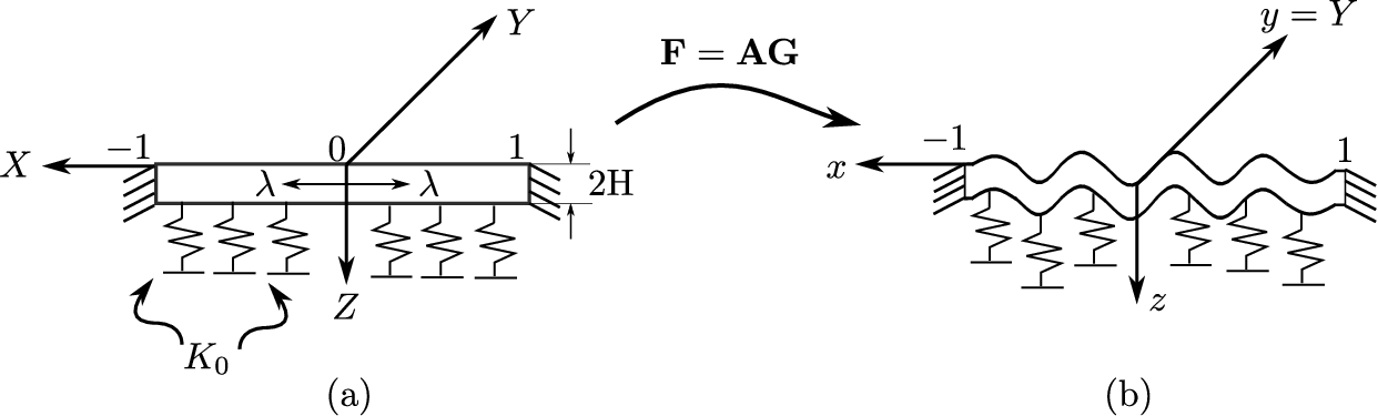
Consider a rectangular plate of thickness clamped at the ends (as shown in Figure 5) subjected to a plane strain in the -direction and a Winkler foundation with effective stiffness at . Analytical results for this problem are derived by Wang et al. 2018. The Winkler foundation allows for analytical solution (Dervaux and Amar 2010). The plate is made up of an incompressible neo-Hookean material growing under uni-axial constant growth field for which the growth tensor takes the form . The Winkler support provides traction only in the transverse direction at the bottom surface of the plate given as where is the ratio of plate thickness to length (in the X direction) i.e., , is the elastic constant of the foundation and is the transverse component of the displacement. We perturb the principal solution scaled by a small parameter ; , where , are the deformed coordinates, and and are the displacements in axial and transverse direction, respectively. Upon substituting this ansatz in (2.11), equating (2.11b) to , and collecting only terms, the governing plate differential equation is given by
| (5.1) |
subjected to clamped boundary conditions, . Here
and where is the ground state shear modulus of the hyperelastic material. We follow the same numerical scheme as described in Section 5.3 and obtained the bifurcation solution by numerically solving the GDE (5.1) for critical value of growth ( responsible for the onset of instability. We compare our numerical results with the existing analytical results using current theory and numerical result using FvK plate theory provided by Wang et al. 2018 in Table 1. The current numerical results are an almost exact match with the analytical solution and very close to the results obtained by the FvK theory.
| Mode number | ||||
|---|---|---|---|---|
| FvK theory | 1.01596 | 1.01712 | 1.01814 | 1.01916 |
| Analytical results (Wang et al. 2018) | 1.01626 | 1.01751 | 1.01839 | 1.01969 |
| Current results | 1.01626 | 1.01751 | 1.01839 | 1.01969 |
5.2 Results for annular plate
The previous Section 4 discussed the possible type of perturbations (axisymmetry and asymmetric), corresponding ODEs and boundary conditions for the stability analysis. In this section, we numerically solve the derived ODEs to determine the critical growth factor at the onset of bifurcation. The numerical strategy used to derive the bifurcation solution is detailed in Section 5.3. We have shown only one set of bifurcation solutions in Subsection 5.3.1 when a plate is perturbed in direction and subjected to IFOC boundary condition. This is to illustrate the stability of buckling solution of the growing plate when perturbed. Then in Subsection 5.4, we compare the bifurcation solution of each type of perturbation considered in Section 4 and investigate the type of perturbation that results in the energetically preferred bifurcation solution. In the next Section 5.5, we have shown the comparison between the preferred bifurcation solutions for both boundary conditions.
5.3 Numerical bifurcation analysis of growing annular plate
In this section, we numerically solve the ODEs obtained in Section 4.1 for the critical growth factor () responsible for the onset of instability. The numerical solutions of the resulting boundary value problems (BVPs) are computed using the compound matrix method (Haughton and Orr 1997; Mehta et al. 2021b) as well as the standard shooting method or determinant method (Haughton and Ogden 1979; Saxena 2018). Both the numerical methods are implemented in Matlab 2018a and the computed results are witin a very small norm. However, the compound matrix method is much faster than the shooting method (Mehta et al. 2021a). Equations are integrated using the ode45 ODE solver that implements an explicit Runga-Kutta method and then the fminsearchbnd optimisation subroutine (D’Errico 2021) based on a Nelder-Mead simplex algorithm is used to minimise the errors.
5.3.1 Bifurcation solution for a plate with clamped outer edge condition
In this section, we evaluate the value of for the first case as discussed in 4.1 i.e., perturbation along direction to demonstrate the behaviour of the bifurcation solution for an annular plate. For this, we numerically solve the system (4.3) subjected to IFOC boundary condition (4.4). The dependence of on the plate thickness () with different radius ratios at various circumferential wavenumbers () is shown in Figure 6. The monotonically increases with suggesting that thicker plates with high bending stiffness require more growth to cause wrinkling instability. Furthermore, the magnitude of decreases with the increase of due to an apparent decrease in the boundary layer effects of the annular plate. We also observe that the critical wavenumber () depends on the thickness, radius ratio, and boundary layer effects of the plate. Higher modes are energetically preferred for the low values whereas lower modes are stable with an increasing value of . For a plate with smaller radius ratio, , the obtained critical wavenumber is in the thin regime (), and in the thick regime (). However, for and , the critical wavenumbers are and , respectively.

5.4 Comparison between axisymmetric and asymmetric bifurcation
Here, we compare the bifurcation solutions for axisymmetric and asymmetric perturbations as discussed in Section 4.1.1 and 4.1.2, respectively. The is calculated by numerically solving the systems (4.7) and (4.11) subjected to the IFOC boundary conditions (4.8) and (4.12), respectively using the compound matrix method. Table 2 shows the dependence of on plate thickness () and plate radius ratio () at the corresponding critical mode number () for each type of the considered perturbation. The bifurcation solution corresponding to axisymmetric (i.e., along ) and asymmetric (i.e., along ) perturbations to principal solution (3.4) follow a trend similar to the solution obtained in Section 5.3.1. The bifurcation solution corresponding to axisymmetric perturbation results in high , thus requiring higher growth factor as compared to bifurcation solution associated with asymmetric perturbations.
For plates with , the bifurcation solution obtained for the perturbation has the minimum energy (highlighted values in Table 2 correspond to lowest values of and therefore the preferred bifurcation solution) suggesting that the asymmetrically perturbed solution is energetically preferred. On the other hand, for a plate with low radius ratio , the bifurcation solution obtained for the perturbation is energetically preferred. However, for small thickness values , difference in the the critical value for each of the perturbation types is very small and it is hard to predict the preferred bifurcation mode. It is also observed that the critical wave number decreases with an increase in for a fixed value of the plate thickness. This is expected since thinner rings (low ) have a larger circumference in relation to their surface area and therefore tend to develop more wrinkles compared to bulkier rings (high ) and is corroborated by the experimental and analytical findings of Mora and Boudaoud 2006 and Liu et al. 2013.
For , the critical load and the corresponding increase with the thickness . For higher values, remains constant but only increases with the thickness . In general higher thickness value results in larger compressive stresses at the bifurcation point due to a larger value of which is discussed in the subsequent section. As a result, bifurcation occurs with a higher wavenumber for as increases. For , the change in with the value is not significant and as a result stays constant.
We conclude that the (asymmetric) type of perturbation is appropriate for the annular plate with moderate and high radius ratio when subjected to IFOC condition as compared to other perturbations. In the subsequent section, we analyse the influence of ICOF boundary condition (i.e., inner edge of the plate is clamped) on the bifurcation solutions obtained using all types of considered perturbations and compare these results with the IFOC results.
|
|
|
|
| ||||||||||||||||||||||||||||||||||
|---|---|---|---|---|---|---|---|---|---|---|---|---|---|---|---|---|---|---|---|---|---|---|---|---|---|---|---|---|---|---|---|---|---|---|---|---|---|
|
|
|
| ||||||||||||||||||||||||||||||||||
|
|
|
| ||||||||||||||||||||||||||||||||||
|
|
|
| ||||||||||||||||||||||||||||||||||
|
|
|
| ||||||||||||||||||||||||||||||||||
|
|
|
|
5.5 Influence of boundary condition on the buckling solution
In this section, we evaluate for an annular plate considering all type of perturbations by numerically solving (4.3), (4.7), and (4.11) subjected to ICOF conditions (4.5), (4.9), and (4.13), respectively and compare with the solutions obtained in the previous section. The values of are compared for each type of perturbation and then we identify the preferred bifurcation solution by studying the lowest value of (at the corresponding ). Table 3 shows the dependence of preferred bifurcation solution (lowest ) on plate thickness () and radius ratio when the growing plate is subjected to ICOF boundary condition. This table also compares the lowest values of of the plate subjected to IFOC condition (highlighted in Table 2) with the obtained ICOF results. We observe that the variation of with plate thickness () and radius ratio () for both the boundary conditions is quite similar. We also observe that for the plates subjected to ICOF boundary condition, the bifurcation solution associated with perturbation have minimum energy and is preferable over other type of perturbations.
Unlike the IFOC case, the values of and increase with for all values of . This can be visualised by plotting the variation of with for various values of in Figure 7a and Figure 7b. The critical wavenumber (corresponding to the minima of these curves) is constant with for the annular plate () subjected to IFOC boundary condition as discussed in previous section. However, the increases with the for fixed using ICOF boundary condition. This suggest that a preferred bifurcation solution (satisfying the ICOF boundary conditions with perturbation) consist of more wrinkles in hoop direction for thicker plates at high value of . The contour plots with normalised displacement demonstrate the number of wrinkles in the circumferential direction at the bifurcation point. For the plate with and subjected to IFOC boundary condition, the critical wavenumber () is 4 and does not change with the thickness. Whereas, for the plate of , subjected to ICOF boundary condition, the is 6 and for the plate with , the is 14 which shows the increase in number of wrinkles with . This is due to the expansion of the unconstrained outer boundary (considering ICOF) with the increase of thickness under growth stretch (). The deformed configuration results in a larger circumference which can accommodate more number of wrinkles in the buckled configuration.
Figure 7c shows the variation of transverse amplitude of the mode shape along the radius of the plate for different thickness at same radius ratio . In the case of IFOC, the mode shape variation remains the same for all plate thickness considered. In the case of ICOF, for thin plates (), the radial extent of wrinkles is considerable i.e., the amplitude variation along the radius is more, whereas for thick plates the amplitude variation is localised at the unconstrained outer edge (as shown in Figure 7b). Thus, in the case of ICOF, the boundary layer effects are observed to be significant for thick plates when compared to thin plates.
Next, we investigate the effect of compressive stress on the wrinkle formation along the boundaries of annular plate. Figure 7d and Figure 7e shows the variation of normalised maximum stress () with the plate radius ratio at different plate thickness values () for IFOC and ICOF boundary conditions, respectively. The blue and red curves represents the dimensionless radial stress () and circumferential stress (), respectively. The variation of maximum stress with aspect ratio shows the similar behaviour for IFOC and ICOF case however, we observe that for IFOC condition, both the and are compressive which promotes the bifurcation where as for ICOF boundary condition, is compressive and is tensile that delays the bifurcation (Mathematical expressions for stresses are detailed in the supplementary document). Here, we plot the maximum stress value to show the dependence of stresses on the geometry of plate. Considering ICOF condition, for a fixed value of , the value of critical growth stretch increases with the increase of thickness (due to increased bending stiffness), as shown in Table 3 which yields high compressive stresses as shown in Figure 7d and Figure 7e which results in more number of wrinkles. Whereas, the converse behaviour of stress is observed with respect to increase in the radius ratio of the annular plate for a fixed value of plate thickness that is the critical stretch value and compressive stresses decrease with the increase in radius ratio suggesting less wrinkles. For plates with low value, both the compressive stress and boundary layer effects govern the wrinkle formation. For plates with high value, only the compressive stress governs the wrinkle formation. Thus the combined effect of compressive stresses and boundary layer effects govern the number of wrinkles and their localization along the boundaries of the thick plate. Also, the results show that the magnitude of and is higher for the bifurcation solution associated with ICOF case when compared to IFOC. For the same geometric parameters and , the value of associated with IFOC condition is at and ICOF condition is at .
|
|
| |||||||||||||||||||||||||
|---|---|---|---|---|---|---|---|---|---|---|---|---|---|---|---|---|---|---|---|---|---|---|---|---|---|---|---|
| 0.03 |
|
|
| ||||||||||||||||||||||||
| 0.05 |
|
|
| ||||||||||||||||||||||||
| 0.1 |
|
|
| ||||||||||||||||||||||||
| 0.15 |
|
|
| ||||||||||||||||||||||||
| 0.2 |
|
|
|

5.5.1 Comparison with computational results for growing annulus
We have discussed in Section 3.2 that current plate theory estimates pre-buckling results for circular ring and annular shell. Now, to test the accuracy of numerical framework, we compare the bifurcation solution of the annular plate using current theory with the computational results for a nearly incompressible (Poisson ratio = 0.495) neo-Hookean growing annulus provided by Groh 2022 using the finite element method. He used a seven-parameter quadrilateral shell element to analyse the growth-induced instability in thin growing shell by implementing the numerical continuation algorithm. In his work, the isotropic planar growth tensor is given as . The prescribed boundary condition were pinned inner edge and free outer edge. He reported the critical value of growth function and wavenumber for growing annulus as and , respectively. For the same parameters, radius ratio (), shell thickness (), and the boundary conditions which are (corresponding to simply supported inner boundary) and (corresponding to free outer boundary), the current incompressible plate theory yields the critical wavenumber with . The two results are relatively close to each other with a small deviation arising due to the non satisfaction of incompressibility constraint in Groh 2022’s formulation.
6 Conclusion
In this work, we have investigated the wrinkling phenomena in growing hyperelastic annular plates using a finite strain asymptotic plate theory. A 3-D plate equilibrium system is reduced to 2-D plate governing system by adopting series expansion along the thickness direction. A homogeneous isotropic growth function is considered as a control parameter in inducing the circumferential instability in an incompressible neo-Hookean annular plate. To validate the 2-D plate framework, we compared the numerical pre-buckling solution for a very thin annular plate with the analytical pre-buckling solution of circular ring. Both the analytical and numerical results are in good agreement. We carried out linear bifurcation analysis with asymmetric (i.e., along and direction) as well as axisymmetric perturbations (i.e., along direction) for two cases of boundary conditions (IFOC and ICOF). The numerical solution of resulting system of ODEs in each case is solved using the compound matrix method. The critical value of growth factor () and the associated wavenumber () is evaluated for each type of perturbation and boundary conditions. We observe that the bifurcation solution corresponding to asymmetric perturbation is preferred for both boundary conditions as it has a lower value of when compared to the axisymmetric perturbation. The bifurcation solutions associated with IFOC and ICOF boundary conditions exhibit a similar behaviour for variation of (at ) with and . However, the magnitude of is lower for the case of IFOC when compared to ICOF due to the presence of compressive radial and circumferential stresses which promotes wrinkling. In addition, for ICOF case, we find that for a fixed value of , the deformed radius and increases with plate thickness resulting in higher compressive stress in circumferential direction which further results in more number of localised wrinkles along the outer circumference of the thicker plate. To test the accuracy of obtained results for annular plate, we compare the bifurcation solution obtained for incompressible annular plate with the existing bifurcation solution for slightly incompressible shell obtained using finite element approach. Both the bifurcation results are close to each other showing the consistency of current plate theory.
Furthermore, we have restricted our study to determine the critical value of growth factor responsible for the onset of wrinkling, however a post-bifurcation analysis may provide insights on the evolution of wrinkle deformation with growth. This is currently being investigated and our findings will be reported in a suitable forum at a later stage.
Acknowledgements
Prashant Saxena acknowledges the financial support of the EPSRC grant no. EP/V030833/1.
References
- Ambrosi et al. (2011) Ambrosi D., Ateshian G.A., Arruda E.M., Cowin S., Dumais J., Goriely A., Holzapfel G.A., Humphrey J.D., Kemkemer R., Kuhl E. et al. “Perspectives on biological growth and remodeling”. Journal of the Mechanics and Physics of Solids, 59(4):863–883 (2011)
- Balbi and Ciarletta (2013) Balbi V. and Ciarletta P. “Morpho-elasticity of intestinal villi”. Journal of the Royal Society Interface, 10(82):20130109 (2013)
- Ben Amar and Goriely (2005) Ben Amar M. and Goriely A. “Growth and instability in elastic tissues”. Journal of the Mechanics and Physics of Solids, 53(10):2284–2319 (2005)
- Bowden et al. (2016) Bowden L., Byrne H., Maini P., and Moulton D. “A morphoelastic model for dermal wound closure”. Biomechanics and modeling in mechanobiology, 15(3):663–681 (2016)
- Budday et al. (2014) Budday S., Steinmann P., and Kuhl E. “The role of mechanics during brain development”. Journal of the Mechanics and Physics of Solids, 72:75–92 (2014)
- Cao and Hutchinson (2012) Cao Y. and Hutchinson J.W. “From wrinkles to creases in elastomers: the instability and imperfection-sensitivity of wrinkling”. Proceedings of the Royal Society A: Mathematical, Physical and Engineering Sciences, 468(2137):94–115 (2012)
- Cao et al. (2012) Cao Y., Jiang Y., Li B., and Feng X. “Biomechanical modeling of surface wrinkling of soft tissues with growth-dependent mechanical properties”. Acta Mechanica Solida Sinica, 25(5):483–492 (2012)
- Cerda (2005) Cerda E. “Mechanics of scars”. Journal of biomechanics, 38(8):1598–1603 (2005)
- Chen and Dai (2020) Chen X. and Dai H.H. “Stress-free configurations induced by a family of locally incompatible growth functions”. Journal of the Mechanics and Physics of Solids, 137:103834 (2020)
- Coen et al. (2004) Coen E., Rolland-Lagan A.G., Matthews M., Bangham J.A., and Prusinkiewicz P. “The genetics of geometry”. Proceedings of the National Academy of Sciences, 101(14):4728–4735 (2004)
- Coman and Haughton (2006) Coman C.D. and Haughton D. “Localized wrinkling instabilities in radially stretched annular thin films”. Acta Mechanica, 185(3):179–200 (2006)
- Coman et al. (2015) Coman C.D., Matthews M.T., and Bassom A.P. “Asymptotic phenomena in pressurized thin films”. Proceedings of the Royal Society A: Mathematical, Physical and Engineering Sciences, 471(2182):20150471 (2015)
- Dai and Liu (2014) Dai H.H. and Liu Y. “Critical thickness ratio for buckled and wrinkled fruits and vegetables”. EPL (Europhysics Letters), 108(4):44003 (2014)
- Dai and Song (2014) Dai H.H. and Song Z. “On a consistent finite-strain plate theory based on three-dimensional energy principle”. Proceedings of the Royal Society A: Mathematical, Physical and Engineering Sciences, 470(2171):20140494 (2014)
- D’Errico (2021)
D’Errico J.
“fminsearchbnd, fminsearchcon
(https://www.mathworks.com/matlabcentral/fileexchange/
8277-fminsearchbnd-fminsearchcon), MATLAB Central File Exchange.” (2021) - Dervaux and Amar (2010) Dervaux J. and Amar M.B. “Localized growth of layered tissues”. IMA journal of applied mathematics, 75(4):571–580 (2010)
- Dervaux et al. (2009) Dervaux J., Ciarletta P., and Ben Amar M. “Morphogenesis of thin hyperelastic plates: a constitutive theory of biological growth in the föppl–von kármán limit”. Journal of the Mechanics and Physics of Solids, 57(3):458–471 (2009)
- Dias et al. (2011) Dias M.A., Hanna J.A., and Santangelo C.D. “Programmed buckling by controlled lateral swelling in a thin elastic sheet”. Physical Review E, 84(3):036603 (2011)
- Dortdivanlioglu et al. (2017) Dortdivanlioglu B., Javili A., and Linder C. “Computational aspects of morphological instabilities using isogeometric analysis”. Computer Methods in Applied Mechanics and Engineering, 316:261–279 (2017)
- Du et al. (2020) Du P., Dai H.H., Wang J., and Wang Q. “Analytical study on growth-induced bending deformations of multi-layered hyperelastic plates”. International Journal of Non-Linear Mechanics, 119:103370 (2020)
- Du et al. (2018) Du Y., Lü C., Chen W., and Destrade M. “Modified multiplicative decomposition model for tissue growth: beyond the initial stress-free state”. Journal of the Mechanics and Physics of Solids, 118:133–151 (2018)
- Du et al. (2019) Du Y., Lü C., Destrade M., and Chen W. “Influence of initial residual stress on growth and pattern creation for a layered aorta”. Scientific reports, 9(1):1–9 (2019)
- Efrati et al. (2009) Efrati E., Sharon E., and Kupferman R. “Elastic theory of unconstrained non-euclidean plates”. Journal of the Mechanics and Physics of Solids, 57(4):762–775 (2009)
- Flynn and McCormack (2008) Flynn C. and McCormack B.A. “A simplified model of scar contraction”. Journal of biomechanics, 41(7):1582–1589 (2008)
- Garikipati et al. (2004) Garikipati K., Arruda E.M., Grosh K., Narayanan H., and Calve S. “A continuum treatment of growth in biological tissue: the coupling of mass transport and mechanics”. Journal of the Mechanics and Physics of Solids, 52(7):1595–1625 (2004)
- Goriely (2017) Goriely A. The mathematics and mechanics of biological growth, volume 45. Springer (2017)
- Goriely and Ben Amar (2005) Goriely A. and Ben Amar M. “Differential growth and instability in elastic shells”. Physical review letters, 94(19):198103 (2005)
- Goriely and Ben Amar (2007) Goriely A. and Ben Amar M. “On the definition and modeling of incremental, cumulative, and continuous growth laws in morphoelasticity”. Biomechanics and modeling in mechanobiology, 6(5):289–296 (2007)
- Groh (2022) Groh R.M. “A morphoelastic stability framework for post-critical pattern formation in growing thin biomaterials”. Computer Methods in Applied Mechanics and Engineering, 394:114839 (2022)
- Haughton and Ogden (1979) Haughton D. and Ogden R. “Bifurcation of inflated circular cylinders of elastic material under axial loading—ii. exact theory for thick-walled tubes”. Journal of the Mechanics and Physics of Solids, 27(5-6):489–512 (1979)
- Haughton and Orr (1997) Haughton D. and Orr A. “On the eversion of compressible elastic cylinders”. International journal of solids and structures, 34(15):1893–1914 (1997)
- Holmes (2019) Holmes D.P. “Elasticity and stability of shape-shifting structures”. Current opinion in colloid & interface science, 40:118–137 (2019)
- Huang et al. (2018) Huang C., Wang Z., Quinn D., Suresh S., and Hsia K.J. “Differential growth and shape formation in plant organs”. Proceedings of the National Academy of Sciences, 115(49):12359–12364 (2018)
- Ionov (2013) Ionov L. “Biomimetic hydrogel-based actuating systems”. Advanced Functional Materials, 23(36):4555–4570 (2013)
- Jia et al. (2018) Jia F., Pearce S.P., and Goriely A. “Curvature delays growth-induced wrinkling”. Physical Review E, 98(3):033003 (2018)
- Jin et al. (2011) Jin L., Cai S., and Suo Z. “Creases in soft tissues generated by growth”. EPL (Europhysics Letters), 95(6):64002 (2011)
- Jones and Mahadevan (2015) Jones G.W. and Mahadevan L. “Optimal control of plates using incompatible strains”. Nonlinearity, 28(9):3153 (2015)
- Kadapa et al. (2021) Kadapa C., Li Z., Hossain M., and Wang J. “On the advantages of mixed formulation and higher-order elements for computational morphoelasticity”. Journal of the Mechanics and Physics of Solids, 148:104289 (2021)
- Kempaiah and Nie (2014) Kempaiah R. and Nie Z. “From nature to synthetic systems: shape transformation in soft materials”. Journal of Materials Chemistry B, 2(17):2357–2368 (2014)
- Khang et al. (2009) Khang D.Y., Rogers J.A., and Lee H.H. “Mechanical buckling: mechanics, metrology, and stretchable electronics”. Advanced Functional Materials, 19(10):1526–1536 (2009)
- Kienzler (2002) Kienzler R. “On consistent plate theories”. Archive of Applied Mechanics, 72(4):229–247 (2002)
- Kuhl (2014) Kuhl E. “Growing matter: a review of growth in living systems”. Journal of the Mechanical Behavior of Biomedical Materials, 29:529–543 (2014)
- Li et al. (2012) Li B., Cao Y.P., Feng X.Q., and Gao H. “Mechanics of morphological instabilities and surface wrinkling in soft materials: a review”. Soft Matter, 8(21):5728–5745 (2012)
- Li et al. (2010) Li B., Huang S.Q., and Feng X.Q. “Buckling and postbuckling of a compressed thin film bonded on a soft elastic layer: a three-dimensional analysis”. Archive of Applied Mechanics, 80(2):175–188 (2010)
- Li et al. (2013) Li B., Xu G.K., and Feng X.Q. “Tissue–growth model for the swelling analysis of core–shell hydrogels”. Soft Materials, 11(2):117–124 (2013)
- Li et al. (2022) Li Z., Wang Q., Du P., Kadapa C., Hossain M., and Wang J. “Analytical study on growth-induced axisymmetric deformations and shape-control of circular hyperelastic plates”. International Journal of Engineering Science, 170:103594 (2022)
- Liang and Mahadevan (2009) Liang H. and Mahadevan L. “The shape of a long leaf”. Proceedings of the National Academy of Sciences, 106(52):22049–22054 (2009)
- Liang and Mahadevan (2011) Liang H. and Mahadevan L. “Growth, geometry, and mechanics of a blooming lily”. Proceedings of the National Academy of Sciences, 108(14):5516–5521 (2011)
- Limbert and Kuhl (2018) Limbert G. and Kuhl E. “On skin microrelief and the emergence of expression micro-wrinkles”. Soft matter, 14(8):1292–1300 (2018)
- Liu et al. (2021) Liu R.C., Liu Y., and Cai Z. “Influence of the growth gradient on surface wrinkling and pattern transition in growing tubular tissues”. Proceedings of the Royal Society of London Series A, 477(2254):20210441 (2021)
- Liu et al. (2020a) Liu Y., Ma W., and Dai H.H. “On a consistent finite-strain plate model of nematic liquid crystal elastomers”. Journal of the Mechanics and Physics of Solids, 145:104169 (2020a)
- Liu et al. (2014) Liu Y., Zhang H., Zheng Y., Zhang S., and Chen B. “A nonlinear finite element model for the stress analysis of soft solids with a growing mass”. International Journal of Solids and Structures, 51(17):2964–2978 (2014)
- Liu et al. (2020b) Liu Y., Zhang Z., Devillanova G., and Cai Z. “Surface instabilities in graded tubular tissues induced by volumetric growth”. International Journal of Non-Linear Mechanics, 127:103612 (2020b)
- Liu et al. (2013) Liu Z., Swaddiwudhipong S., and Hong W. “Pattern formation in plants via instability theory of hydrogels”. Soft Matter, 9(2):577–587 (2013)
- Mehta et al. (2021a) Mehta S., Raju G., Kumar S., and Saxena P. “Instabilities in a compressible hyperelastic cylindrical channel due to internal pressure and external constraints” (2021a)
- Mehta et al. (2021b) Mehta S., Raju G., and Saxena P. “Growth induced instabilities in a circular hyperelastic plate”. International Journal of Solids and Structures, 226:111026 (2021b)
- Mihai and Goriely (2020) Mihai L.A. and Goriely A. “A plate theory for nematic liquid crystalline solids”. Journal of the Mechanics and Physics of Solids, 144:104101 (2020)
- Mora and Boudaoud (2006) Mora T. and Boudaoud A. “Buckling of swelling gels”. The European Physical Journal E, 20(2):119–124 (2006)
- Moulton and Goriely (2011) Moulton D. and Goriely A. “Circumferential buckling instability of a growing cylindrical tube”. Journal of the Mechanics and Physics of Solids, 59(3):525–537 (2011)
- Nassar et al. (2012) Nassar D., Letavernier E., Baud L., Aractingi S., and Khosrotehrani K. “Calpain activity is essential in skin wound healing and contributes to scar formation”. PloS one, 7(5):e37084 (2012)
- Papastavrou et al. (2013) Papastavrou A., Steinmann P., and Kuhl E. “On the mechanics of continua with boundary energies and growing surfaces”. Journal of the Mechanics and Physics of Solids, 61(6):1446–1463 (2013)
- Pezzulla et al. (2016) Pezzulla M., Smith G.P., Nardinocchi P., and Holmes D.P. “Geometry and mechanics of thin growing bilayers”. Soft matter, 12(19):4435–4442 (2016)
- Raybaud and Widjaja (2011) Raybaud C. and Widjaja E. “Development and dysgenesis of the cerebral cortex: malformations of cortical development”. Neuroimaging Clinics, 21(3):483–543 (2011)
- Rodriguez et al. (1994) Rodriguez E.K., Hoger A., and McCulloch A.D. “Stress-dependent finite growth in soft elastic tissues”. Journal of biomechanics, 27(4):455–467 (1994)
- Rogers et al. (2010) Rogers J.A., Someya T., and Huang Y. “Materials and mechanics for stretchable electronics”. science, 327(5973):1603–1607 (2010)
- Saez (2016) Saez P. “On the theories and numerics of continuum models for adaptation processes in biological tissues”. Archives of computational methods in engineering, 23(2):301–322 (2016)
- Saxena (2018) Saxena P. “Finite deformations and incremental axisymmetric motions of a magnetoelastic tube”. Mathematics and Mechanics of Solids, 23(6):950–983 (2018)
- Steele (2000) Steele C.R. “Shell stability related to pattern formation in plants”. Journal of Applied Mechanics, 67(2):237–247 (2000)
- Stein-Montalvo et al. (2019) Stein-Montalvo L., Costa P., Pezzulla M., and Holmes D.P. “Buckling of geometrically confined shells”. Soft Matter, 15(6):1215–1222 (2019)
- Swain and Gupta (2015) Swain D. and Gupta A. “Interfacial growth during closure of a cutaneous wound: stress generation and wrinkle formation”. Soft matter, 11(32):6499–6508 (2015)
- Swain and Gupta (2016) Swain D. and Gupta A. “Mechanics of cutaneous wound rupture”. Journal of biomechanics, 49(15):3722–3730 (2016)
- Tallinen and Biggins (2015) Tallinen T. and Biggins J.S. “Mechanics of invagination and folding: Hybridized instabilities when one soft tissue grows on another”. Physical Review E, 92(2):022720 (2015)
- Terwagne et al. (2014) Terwagne D., Brojan M., and Reis P.M. “Smart morphable surfaces for aerodynamic drag control”. Advanced materials, 26(38):6608–6611 (2014)
- Vandiver and Goriely (2009) Vandiver R. and Goriely A. “Differential growth and residual stress in cylindrical elastic structures”. Philosophical Transactions of the Royal Society A: Mathematical, Physical and Engineering Sciences, 367(1902):3607–3630 (2009)
- Wang et al. (2019a) Wang F.F., Steigmann D.J., and Dai H.H. “On a uniformly-valid asymptotic plate theory”. International Journal of Non-Linear Mechanics, 112:117–125 (2019a)
- Wang et al. (2022) Wang J., Li Z., and Jin Z. “A theoretical scheme for shape-programming of thin hyperelastic plates through differential growth”. Mathematics and Mechanics of Solids, page 10812865221089694 (2022)
- Wang et al. (2016) Wang J., Song Z., and Dai H.H. “On a consistent finite-strain plate theory for incompressible hyperelastic materials”. International Journal of Solids and Structures, 78:101–109 (2016)
- Wang et al. (2018) Wang J., Steigmann D., Wang F.F., and Dai H.H. “On a consistent finite-strain plate theory of growth”. Journal of the Mechanics and Physics of Solids, 111:184–214 (2018)
- Wang et al. (2019b) Wang J., Wang Q., Dai H.H., Du P., and Chen D. “Shape-programming of hyperelastic plates through differential growth: an analytical approach”. Soft matter, 15(11):2391–2399 (2019b)
- Wang and Zhao (2015) Wang Q. and Zhao X. “A three-dimensional phase diagram of growth-induced surface instabilities”. Scientific reports, 5(1):1–10 (2015)
- Wang et al. (2020) Wang T., Yang Y., Fu C., Liu F., Wang K., and Xu F. “Wrinkling and smoothing of a soft shell”. Journal of the Mechanics and Physics of Solids, 134:103738 (2020)
- Wiggs et al. (1997) Wiggs B.R., Hrousis C.A., Drazen J.M., and Kamm R.D. “On the mechanism of mucosal folding in normal and asthmatic airways”. Journal of Applied Physiology, 83(6):1814–1821 (1997)
- Wu and Ben Amar (2015) Wu M. and Ben Amar M. “Growth and remodelling for profound circular wounds in skin”. Biomechanics and modeling in mechanobiology, 14(2):357–370 (2015)
- Yang et al. (2021) Yang P., Fang Y., Yuan Y., Meng S., Nan Z., Xu H., Imtiaz H., Liu B., and Gao H. “A perturbation force based approach to creasing instability in soft materials under general loading conditions”. Journal of the Mechanics and Physics of Solids, 151:104401 (2021)
- Yu et al. (2020) Yu X., Fu Y., and Dai H.H. “A refined dynamic finite-strain shell theory for incompressible hyperelastic materials: equations and two-dimensional shell virtual work principle”. Proceedings of the Royal Society A, 476(2237):20200031 (2020)
- Zheng et al. (2019) Zheng Y., Wang J., Ye H., Liu Y., and Zhang H. “A solid-shell based finite element model for thin-walled soft structures with a growing mass”. International Journal of Solids and Structures, 163:87–101 (2019)
Appendix A Appendix: Expression for Piola stress and unknown variables
The series expansion of deformation gradient (), elastic deformation (), inverse transpose of Growth tensor () and Piola Kirchhoff () tensor are given by
| (A.1) | |||||
For an incompressible neo-Hookean material elastic strain energy function is and the associated Piola Kirchhoff stress is given as, . Then, the first term in right side of the expression for in (A.1) is obtained as
| (A.2) |
By using bottom traction condition, and substituting the expression for (see (2.6)) in (A.2) we obtain
| (A.3) |
where , , and . In this work, we use in place of which is given as
| (A.4) |
Using incompressibility constraint det, we obtain which result in
| (A.5) |
where . Using (A.3) we obtain the explicit expression for
| (A.6) |
To obtain the explicit expression for we substitute (A.6) into (A.5) which yields
| (A.7) |
Using Eq. (A.7), we obtain the expression for which is
| (A.8) |
where is given by (A). On substituting in (A.6) we obtain explicit expressions for , , and as
| (A.9) |