Transverse Vector Decomposition Method for Analytical Inversion of Exoplanet Transit SpectraJournal: ApJ jupyter (Kluyver et al. 2016), matplotlib (Hunter 2007), numpy (van der Walt et al. 2011), plotly (Inc. 2015), scipy (Virtanen et al. 2020).

Two and a half decades after the discovery of the first extrasolar system planet, the number of known exoplanets is now into the thousands¹¹ 1 NASA Exoplanet Archive, https://exoplanetarchive.ipac.caltech.edu/.. After the initial boom of discoveries based on the radial velocity method (Wright 2018; Perryman 2018), the current detections are mostly done using transit observations, where a planet is identified while passing in front of the host star, blocking a small fraction of the stellar flux (Henry et al. 2000; Charbonneau et al. 2000). Subsequently, some of the transiting planets are targeted for spectroscopic studies and the transit is recorded at different wavelengths (Schneider 1994; Seager & Sasselov 2000). A number of current and planned large-scale planetary surveys are based on observing planetary transits at different wavelengths, thus providing spectral information about the composition and the structure of the atmosphere of the planet (Madhusudhan 2019).

During a transit event, a planet blocks a certain fraction, $M(\lambda)$, of the original stellar flux $F_{O}(\lambda)$,

where $F_{T}(\lambda)$ is (the minimum of) the observed flux during transit at a given wavelength $\lambda$, $R_{S}$ is the stellar radius, and the transit radius $R_{T}(\lambda)$ is the radius of the equivalent solid disk blocking the same amount of light. The key feature of (1) is the dependence of the transit depth $M(\lambda)$ on the observed wavelength $\lambda$, reflecting the differential absorption properties of the atmosphere due to its chemical composition. This allows for detection of atmospheric gasses with strong absorption lines in the probed wavelength range. In addition, the transit spectrum also contains information about the physical characteristics of the planet like its size, temperature, gravity, atmospheric pressure, etc.

The primary goal of exoplanet transit spectroscopy is the inversion of the observed spectrum in order to retrieve the parameters of the planet and its atmosphere (Fisher & Heng 2018; Cobb et al. 2019; Barstow & Heng 2020; Kitzmann et al. 2020; Harrington et al. 2021; Cubillos et al. 2021; Blecic et al. 2021; Welbanks & Madhusudhan 2021a; Welbanks & Madhusudhan 2021b). This inversion process inevitably relies on a forward model (FM), which, for a given set $\mathcal{S}$ of planet parameters, can predict the observed transit radius at each wavelength:

The inverse problem corresponding to the forward model (2) can then be formulated as follows: given the measured spectrum $R_{T}(\lambda)$, derive the values of the planet-specific parameters. This is a difficult challenge due to intrinsic theoretical complications: first of all, the problem is highly non-linear and does not easily lend itself to simple inversion methods from linear algebra; furthermore, there exist several directions of degenerate solutions in the parameter space which lead to equally plausible transit spectra. In this paper we shall focus on overcoming these theoretical challenges, leaving aside the additional observational complications due to instrumental noise, spectral resolution, etc.

The standard approach is to solve the inversion problem numerically. Classical inversion methods extensively used in analyzing infrared spectra from remote sensing of the Earth and Solar System planets are described in Hanel et al. 2003 and are based on linearizing the problem. More recent approaches incorporate various machine learning (ML) techniques (Márquez-Neila et al. 2018; Zingales & Waldmann 2018; Cobb et al. 2019; Oreshenko et al. 2020; Fisher et al. 2020; Himes et al. 2020b; Himes et al. 2020c; Guzmán-Mesa et al. 2020; Nixon & Madhusudhan 2020; Himes et al. 2020a; Yip et al. 2021; Ardevol Martinez et al. 2022) (for a recent comparative review, see Barstow et al. 2020). The main disadvantages of the numerical ML approach are: i) the ML model is in principle a black box which hides the relevant physics and is not easily interpretable (Nixon & Madhusudhan 2020; Yip et al. 2021); ii) the ML model does not learn directly the relevant physics, but only the (finite amount of) data generated by the forward model, which introduces additional uncertainties during the training process (Matchev et al. 2020).

On the other hand, less has been done in terms of analytical approaches to the inverse problem. The first step in this direction would be to replace the numerical forward model (2) with analytical expressions which capture the relevant physics (Brown 2001; Hubbard et al. 2001; Burrows et al. 2003; Fortney 2005; Benneke & Seager 2012; de Wit & Seager 2013; Griffith 2014; Vahidinia et al. 2014; Heng & Showman 2015; Bétrémieux & Swain 2017; Heng & Kitzmann 2017; Heng 2019) and can then be possibly inverted. The analytical formulas typically rely on simplifying assumptions and approximations,.e.g, spherical symmetry, isothermal atmosphere, isobaric approximation, constant specific gravity, etc. Nevertheless, these theoretical results agree well with the numerical forward models and allow for better understanding of the underlying physics and of the intrinsic parameter degeneracies present in the problem (Griffith 2014; Heng & Kitzmann 2017; Welbanks & Madhusudhan 2019; Matchev et al. 2021).

The main goal of this paper is to push the limits of the analytical approach by applying ideas from vector algebra and analytical geometry to disentangle the parameter dependencies within the forward model and provide a clean measurement of the relative chemical abundances of the absorbers present in the atmosphere. This allows for direct and meaningful comparisons of the atmospheric chemical compositions of different exoplanets, independent of the individual physical planet parameters.

The paper is organized as follows. In section II we describe a typical forward model and introduce the relevant parameters. In section III we review some of the existing analytical approximations in the literature, highlighting their generic features which will be relevant for our discussion. In section IV we describe our analytical inversion procedure which results in the measurement of the relative chemical abundances and two combinations of planet-specific physical parameters. In sections V, VI, VII and VIII we illustrate our method with several toy examples of increasing complexity. In section IX we present our summary and conclusions.

The planet-specific input parameters to the forward model can be categorized into the following three groups:

• •

  Physical parameters. These are parameters which refer to the physical characteristics of the planet or the observational geometry: radius $R_{S}$ of the host star, atmospheric temperature $T$, specific gravity $g$ and reference pressure level $P_{0}$ at a given planet radius $R_{0}$ corresponding to an optically thick atmosphere along the line of sight (Heng & Kitzmann 2017).

• •

  Chemical composition parameters. These are parameters which refer to the chemical composition of the planet atmosphere. The mean molecular mass $\bar{m}$ is determined by the major gas components (e.g., hydrogen and helium for hot Jupiters). The attenuation of the stellar light depends on the volume mixing ratio $X_{a}=n_{a}/n$ (or equivalently, the number density $n_{a}$) and the molecular mass $m_{a}$ of each individual absorber, where $a=1,2,\ldots,N_{abs}$ and $n$ is the total atmospheric number density.

• •

  Wavelength-dependent parameters. These include the cloud opacity $\kappa_{cl}(\lambda)$ and the absorption coefficients $\chi_{a}(\lambda)$ for the individual absorbers. In principle, these parameters can be viewed as a subset of the chemical composition parameters, but here we would like to emphasize their wavelength dependence. Note that the absorption coefficients $\chi_{a}$ in principle depend not only on the wavelength, but also on temperature and (to a lesser extent) on pressure.

With those preliminaries, we can now express the forward model (2) more concretely as

Note that not all of the listed inputs are a priori unknown. For example, for a given constituent $a$, its molecular mass $m_{a}$ and absorption coefficients $\chi_{a}(\lambda)$ are known physical constants. In addition, alternative astronomical observations may provide independent constraints on some of the other input parameters. However, to be completely general, in this paper we shall not rely on such additional observations and will instead treat all planet-specific input parameters (i.e., everything except for the known physical constants $m_{a}$ and $\chi_{a}(\lambda)$) as a priori unknown.

The general expression (3) for the FM can be further simplified by noting that the absorption of the individual gases enters the model only through the total atmospheric opacity

where $N_{abs}$ is the number of absorbers considered in the model. Without any loss of generality, the forward model (3) can then be rewritten as

in terms of the seven input parameters $R_{S}$, $R_{0}$, $T$, $P_{0}$, $g$, $\bar{m}$ and $\kappa(\lambda)$ (Matchev et al. 2021).

Equations (4) and (5) define the general setup for the inverse problem under consideration in this paper. In this section we narrow down the possible analytical forms of the forward model (5).

The first simplification arises due to standard dimensional analysis (Langhaar 1951; Barenblatt 1996). Matchev et al. 2021 showed that, again without any loss of generality, the analytical expression behind the forward model (5) must be of the form

where $H$ is the pressure scale height

$k_{B}$ is the Boltzmann constant and $f$ is an unspecified function of dimensionless quantities only, i.e., of the four dimensionless Pi groups

listed as its arguments, plus possibly some numerical dimensionless mathematical constants like $\pi$, $e$, etc. In order to provide the necessary length dimensions for $R_{T}$, in eq. (6) we singled out $R_{S}$ as a prefactor; the same role could in principle be played by $H$ or $R_{0}$ (the latter choice was the one made in Matchev et al. 2021). Here we find it convenient to work with $R_{S}$ because the transit depth $M$ is quoted in terms of the ratio $R_{T}/R_{S}$, see eq. (1).

Matchev et al. 2021 also showed that $\pi_{4}$ is not a relevant parameter in the problem and can be safely dropped. The end result from the dimensional analysis can therefore be written as

To proceed further, one has to perform explicit theoretical calculations which would reveal the specific form of the function $f$. In order to obtain relatively simple analytical results, one typically has to make some simplifying assumptions. In the case of an isothermal, radially symmetric atmosphere Heng & Kitzmann 2017 obtained a simple analytical expression which can be written in analogy to (9) as

where $\gamma_{E}=0.577215665$ is the Euler–Mascheroni constant,

is the optical thickness of the atmosphere along the line of sight at the reference radius $R_{0}$ and

is the exponential integral of the first order with argument $\tau_{0}$.

For an optically thick atmosphere (large $\tau_{0}$), the $E_{1}$ term is negligible and (10) simplifies to

which is consistent with the general result (9). In the rest of the paper, we shall use the parametrization (13) for illustration of our inversion procedure.

In general, a transit spectrum is taken at different wavelengths, binned in accordance with the spectral resolution of the instrument. Let $N_{bin}$ be the number of spectral bins whose central values form the wavelength vector array

As pictured in this equation, in the remainder of this paper we shall be using vector notation to represent quantities with $N_{bin}$ components, i.e., variables whose values depend on the wavelength $\lambda$. For example, the vector array containing the $N_{bin}$ measured transit radii will be denoted as

Since a transit event measures not $\vec{R}_{T}$ itself, but the ratio $\vec{R}_{T}/R_{S}$ (see eq. (1)), we shall simplify the notation by defining

The dimensionless vector $\vec{r}$ contains the full information about a given transit observation. In our approach, any given transit spectrum is represented by a single point in the $N_{bin}$-dimensional spectral space and $\vec{r}$ is nothing but the position vector of this point, measured from the origin.

An important direction in the $N_{bin}$-dimensional spectral space is given by the universal vector

which points in the direction of perfectly flat transit spectra which show no variation with wavelength. This case could correspond to a planet without any atmosphere, or to an atmosphere dominated by gray clouds, whose opacity is independent of wavelength and can therefore be written as

The absorption coefficients $\chi_{a}(\lambda)$ of the individual absorbers are wavelength dependent and should therefore also be organized into a vector array. However, since absorption coefficients have physical dimensions, we would like to factor out a dimensionful constant $\chi$ which renders the remaining coefficients $\xi_{a}(\lambda)$ dimensionless:

The actual numerical value of $\chi$ is not important and can be chosen for convenience, the simplest choice is simply $\chi=1\ \frac{\rm m^{2}}{\rm kg}$ in SI units. With those conventions, the total opacity (4) becomes

With the new vector array notation, the main result (13) for the transit spectrum can be rewritten as

where in the last term the logarithm function acts component-wise on the vector array $\vec{\kappa}$ as follows

producing a new vector array, as suggested by the long right arrow above the function name. This operation is identical to the way universal functions act on numpy arrays, but unfortunately, there is no established formal mathematical notation for it, and we shall use the long arrow notation depicted in eq. (22).

Let us now work out in detail the last term in eq. (21). First, let us simplify the notation by incorporating the cloud opacity term into the sum in eq. (20). Defining

we can treat the clouds as the $a=0$ absorber and rewrite (20) in a more compact form

Now substituting this into (21), we have

where to arrive at the second line we have multiplied and divided the argument of the logarithm in the last term with the quantity

which is the total mass mixing ratio of all absorbers.

To further simplify the notation, let us introduce the relative mass mixing ratios $\omega_{a}$ for the different absorbers (which for brevity we shall simply refer to as “weights”), which can be written in several equivalent ways:

where the mass mixing ratio $\mu_{a}$, the volume mixing ratio $X_{a}$, the mass density $\rho_{a}$ and the number density $n_{a}$ of each absorber are related by

and $n$ is the atmospheric number density, so that $n\bar{m}$ is the (mass) density of the atmosphere. By definition, the weights $\omega_{a}$ are normalized to one:

This allows us to rewrite (25b) in the form

Before proceeding with the last step of the analysis, let us take stock of what we have been able to accomplish with the last equation. The $N_{bin}$-dimensional vector $\vec{r}$ representing the measured transit spectrum has been decomposed into two components with the help of the dimensionless vectors $\vec{u}$ and $\vec{\xi}_{a}$. The first component in (30) is along the universal vector $\vec{u}$ and depends on all of the input parameters. The second component in (30) is constructed out of the known dimensionless vectors $\vec{\xi}_{a}$ and its direction is entirely determined by the dimensionless chemical composition weights $\omega_{a}$, while its magnitude in addition depends on the ratio $H/R_{S}$. Our main goal will be to measure these components from the data and thus determine the relative chemical composition $\omega_{a}$, the $H/R_{S}$ ratio and the combination of parameters specifying the component of $\vec{r}$ along $\vec{u}$.

Note that the two components in (30) are not orthogonal, since the vectors $\vec{\xi}_{a}$ are not necessarily orthogonal to $\vec{u}$ (in fact, $\vec{\xi}_{0}$ is $\vec{u}$ itself). Therefore, the next step is to decompose the (dimensionless) vector appearing in the last term of (30)

into a longitudinal component $\vec{L}_{\parallel}$ along $\vec{u}$ and a transverse component $\vec{L}_{\perp}$ orthogonal to $\vec{u}$:

where $\hat{u}\equiv\vec{u}/\sqrt{N_{bin}}$ is a unit vector along $\vec{u}$. Substituting (31) and (32) into (30), we get

This is our main result. We are now ready to perform the desired measurements with the following simple algorithm, whose starting point is the observed spectrum $\vec{r}$:

1. 1.

   Compute the $\parallel$ component of $\vec{r}=\vec{R}_{T}/R_{S}$. The first step is to project the measured transit spectrum vector $\vec{r}$ onto the universal direction $\vec{u}$. This results in

   $$r_{\parallel}\equiv\vec{r}\cdot\hat{u}=\biggl\{\frac{R_{0}}{R_{S}}+\frac{H}{R_{S}}\biggl[\gamma_{E}+\frac{\vec{L}\cdot\vec{u}}{N_{bin}}+\ln\biggl(\mu_{abs}\frac{P_{0}\chi}{g}\sqrt{2\pi\frac{R_{0}}{H}}\biggr)\biggr]\biggr\}\sqrt{N_{bin}}.$$

   (34)

   The left-hand side is an experimentally observed quantity, which is equal to $\sqrt{N_{bin}}$ times the average of the spectrum across all wavelengths (this average is an informative quantity — for example, in Matchev et al. 2022 it was shown to be the first principal component of synthetic datasets of transit spectra). The right-hand side of this equation is a theoretical quantity (i.e., function of input planet-specific parameters) which is the theoretical interpretation of this measurement.

2. 2.

   Compute the $\perp$ component of $\vec{r}=\vec{R}_{T}/R_{S}$. Next we obtain the component of $\vec{r}$ orthogonal to $\vec{u}$ by simply subtracting the mean:

   $$\vec{r}_{\perp}\equiv\vec{r}-r_{\parallel}\hat{u}=\frac{H}{R_{S}}\,\vec{L}_{\perp}(\omega_{a}).$$

   (35)

   Once again, the left-hand side is an experimentally observable quantity, in this case an $(N_{bin}-1)$-dimensional vector lying within the $(N_{bin}-1)$-dimensional hyperplane orthogonal to $\vec{u}$. Note that the right-hand side depends on relatively few input parameters, namely, the relative mass mixing ratios $\omega_{a}$ of the absorbers and on the ratio $H/R_{S}$. We shall now proceed to determine those parameters independently.

3. 3.

   Determine the relative mass mixing ratios $\omega_{a}$. The key observation at this point is that the direction of the transverse vector $\vec{L}_{\perp}(\omega_{a})$ is completely determined by the dimensionless weights $\omega_{a}$. At the same time, this direction is already known from the measurement (35) of $\vec{r}_{\perp}$. Therefore, all parameters $\omega_{a}$ can be simultaneously determined by requiring that the measured vector $\vec{r}_{\perp}$ is in the same direction as $\vec{L}_{\perp}(\omega_{a})$. This can be accomplished, for example, by scanning over all possible trial values $\tilde{\omega}_{a}$ until the two vectors point in the same direction, i.e., until the relevant dot product is maximized:

   $$\omega_{a}=\argmax_{\tilde{\omega}_{a}\in[0,1]}\left(\vec{r}_{\perp}\cdot\left(\frac{\vec{L}_{\perp}(\tilde{\omega}_{a})}{|\vec{L}_{\perp}(\tilde{\omega}_{a})|}\right)\right).$$

   (36)

   As indicated in eq. (36), in the rest of the paper we shall use a tilde to denote trial values for different parameters. On the other hand, retrieved parameter values will carry no tilde.

4. 4.

   Determine the ratio $H/R_{S}$. Once the relative weights are found from (36), the vector $\vec{L}_{\perp}(\omega_{a})$ is fully determined. Then the ratio $H/R_{S}$ can be obtained by simply dividing the magnitudes (or the corresponding individual components) of $\vec{r}_{\perp}$ and $\vec{L}_{\perp}(\omega_{a})$:

   $$\frac{H}{R_{S}}=\frac{\left|\vec{r}_{\perp}\right|}{|\vec{L}_{\perp}(\omega_{a})|}.$$

   (37)

To review the bidding so far, the above algorithm has allowed us to measure a total of $N_{abs}+1$ degrees of freedom, namely: i) the parameter combination in the right-hand side of eq. (34), ii) the ratio $H/R_{S}$ and iii) the $N_{abs}-1$ independent degrees of freedom contained in the relative mass mixing ratios $\omega_{a}$ (recall that one degree of freedom there is removed by the normalization condition (29)). Therefore, a necessary condition for being able to fully determine all these degrees of freedom is that the number of bins in the transit spectrum is at least that many:

In the next few sections we shall illustrate the algorithm described above with some simple yet non-trivial examples: $N_{bin}=3$ and $N_{abs}=2$ in section V, $N_{bin}=4$ and $N_{abs}=3$ in section VI and $N_{bin}=3$ and $N_{abs}=3$ in section VII. In those cases, our inversion procedure can be easily visualized due to the relatively low number of bins. Then in section VIII we shall consider a more realistic example with $N_{bin}=13$ and $N_{abs}=3$. In all of these examples, we shall use common fixed values for the following planet-specific parameters: $R_{0}=1.79R_{J}$, $R_{S}=1.57R_{\odot}$, $g=9.77$ m/s², $P_{0}=10$ bar, $\bar{m}=2.4\,m_{\rm amu}$, where $m_{\rm amu}=1.660539040\times 10^{-27}$ kg is the atomic mass unit, which are consistent with those inferred for WASP-12b (Márquez-Neila et al. 2018). Then for each model, we shall be choosing a study point defined by the masses $m_{a}$, the volume mixing ratios $X_{a}$ and the dimensionless absorption coefficients $\vec{\xi}_{a}$ (at a given temperature $T$) for the respective number of absorbers $N_{abs}$ and number of wavelength bins $N_{bin}$. Then we shall apply our algorithm to recover the values of the input parameters for the respective study point.

We start with a simple toy example with $N_{bin}=3$ bins in the transit spectrum and $N_{abs}=2$ absorbers in the atmosphere. The two absorbers will be denoted as $A$ and $B$ and will be taken to have the following parameters at $T=2000$ K:

The resulting spectrum from eq. (13) is

which corresponds to a vector $\vec{r}$ in the 3-bin spectral space

We now decompose this vector into a longitudinal and transverse components:

where the unit vectors $\hat{u}$, $\hat{e}_{1}$ and $\hat{e}_{1}$ form an orthonormal right-handed system. The unit vector $\hat{u}$ was already discussed earlier, while the unit vectors $\hat{e}_{1}$ and $\hat{e}_{2}$ parametrize the transverse plane and one possible choice is as follows

Dotting (41) into (43), we find the three components of $\vec{r}$

Using the numerical values for the planet parameters listed at the end of section IV, one can easily verify that the obtained numerical value for $r_{\parallel}$ is precisely as predicted by the right-hand side of eq. (34). This completes Steps 1 and 2 of the algorithm.

The measurement of the mixing ratios $\omega_{A}$ and $\omega_{B}$ via Step 3 is illustrated in the two panels of Figure 1. The direction of $\vec{r}_{\perp}$ in the transverse plane can be found from the measured components (44) and is given by the polar angle

This direction is indicated by a diagonal dotted line in the left panel of Figure 1 and by a horizontal dashed line in the right panel of Figure 1. In order to find the weights $\omega_{A}$ and $\omega_{B}$, we need to build the set of vectors (31) in terms of the trial values $\tilde{\omega}_{A}$ and $\tilde{\omega}_{B}$, i.e.

and find which one of them has a transverse component $\vec{L}_{\perp}(\tilde{\omega}_{A},\tilde{\omega}_{B})$ matching the direction of $\vec{r}_{\perp}$. This simple exercise is also illustrated in Figure 1. The colored points in the left panel of the figure represent the family of vectors $\vec{L}_{\perp}(\tilde{\omega}_{A},\tilde{\omega}_{B})$, color coded by the trial value of $\tilde{\omega}_{A}$ (recall that in this toy example $\tilde{\omega}_{B}$ will be simply given by $1-\tilde{\omega}_{A}$). The gray arrows depict five $\vec{L}_{\perp}$ vectors corresponding to five representative trial values of $\tilde{\omega}_{A}=\{1.0,0.90,0.50,0.10,0.0\}$ (from left to right), and the color coding gives all intermediate trial values of $\tilde{\omega}_{A}$. The direction of $\vec{r}_{\perp}$ intersects the $\vec{L}_{\perp}$ family at the point marked with the star symbol, which reveals the true value of $\omega_{A}$ as $\omega_{A}=0.833$, in precise agreement with the input value in (39a).

The right panel in Figure 1 shows an alternative representation of the same measurement. Since the family of $\vec{L}_{\perp}(\tilde{\omega}_{A},\tilde{\omega}_{B})$ vectors does not involve any other planet-specific parameters, the relationship between the trial mass mixing ratio $\tilde{\omega}_{A}$ and the corresponding $\vec{L}_{\perp}(\tilde{\omega}_{A},\tilde{\omega}_{B})$ direction can be built up in advance, as shown in the right panel of Figure 1, where we kept the color-coding for convenience only (it simply tracks the horizontal axis). Then, once the direction of $\vec{r}_{\perp}$ is known from (45), we can directly read off the true value of the mixing ratio $\omega_{A}$ from the horizontal axis, as illustrated with the dashed lines.

Once the value of $\omega_{A}$ is known, in Step 4 of the algorithm we construct the vector

which allows us to compute the ratio $H/R_{S}$ in several equivalent ways:

which was precisely the input value in this example.

This concludes the demonstration of the algorithm in this very first toy example. The algorithm reproduced exactly (within machine precision) the input values for the fractional chemical abundance of the two components ($\omega_{A}$ and $\omega_{B}$), the ratio $H/R_{S}$ and the spectral average $r_{\parallel}$. The algorithm would work for any number of bins $N_{bin}$ and any number of chemical absorbers $N_{abs}$, yet the simplicity of this toy example allowed for easy visualization and comprehensive step-by-step demonstration of the main steps of the algorithm. In the following two sections we shall consider more complicated and more realistic examples, skipping some of the details already seen here and instead focusing on the new elements in those examples.

In this section we shall consider a slightly more complex example with $N_{bin}=4$ bins in the transit spectrum and $N_{abs}=3$ absorbers in the atmosphere. The wavelength-dependent vector arrays now have 4 components. The three absorbers will be denoted as $A$, $B$ and $C$ and will be taken to have the following parameters (at $T=2000$ K)

With those inputs, the transit 4-bin spectrum is

which corresponds to the vector $\vec{r}$

which we decompose as

onto the four orthonormal vectors

resulting in the four components

It is easy to check that the measured component $r_{\parallel}$ along the universal vector $\vec{u}$ once again exactly matches the prediction from the theoretical formula (34). This time the transverse vector $\vec{r}_{\perp}$ is three-dimensional. In order to extract the chemical composition from its direction, we form the vector family

parametrized in terms of the trial values $\tilde{\omega}_{A}$, $\tilde{\omega}_{B}$ and $\tilde{\omega}_{C}=1-\tilde{\omega}_{A}-\tilde{\omega}_{B}$, and project it on the transverse space as

The family of transverse vectors $\vec{L}_{\perp}(\tilde{\omega}_{a})$ is visualized in Figure 2 in complete analogy with Figure 1. We scan $\tilde{\omega}_{A}$ and $\tilde{\omega}_{B}$ on a regular grid with 200 points in each direction and show the resulting grid of transverse vectors $\vec{L}_{\perp}(\tilde{\omega}_{a})$. The tips of the vectors $\vec{L}_{\perp}(\tilde{\omega}_{a})$ outline a two-dimensional triangularly-shaped surface in the three-dimensional transverse space, whose corners $A$, $B$ and $C$ correspond to $\tilde{\omega}_{A}=100\%$, $\tilde{\omega}_{B}=100\%$ and $\tilde{\omega}_{C}=100\%$, respectively. The surface is color-coded by the value of $\tilde{\omega}_{B}$ in the left panel and $\tilde{\omega}_{C}$ in the right panel. The origin O of the coordinate system is marked with the $\times$ symbol and the dotted line originating from O shows the measured direction of $\vec{r}_{\perp}$ according to (54). This line intersects the plotted surface at the point marked with the $\star$ symbol, which reveals the location of the vector $\vec{L}_{\perp}(\omega_{a})$ built from the true values of the mass mixing ratios $\omega_{a}$. The length of this vector in turn reveals the ratio $H/R_{S}$ according to (37). Once again, the described procedure resulted in exact retrieval of the parameters $\omega_{a}$, $H/R_{S}$ and $r_{\parallel}$ (the precision is only limited by the resolution of the $\tilde{\omega}_{a}$ scan which can be taken to be arbitrarily precise).

Since in this example we have three absorbers with relative weights $\omega_{a}$ subject to $\omega_{A}+\omega_{B}+\omega_{C}=1$, the appropriate generalization of the right panel in Figure 1 is a ternary plot, as illustrated in Figure 3. Each point on the plot represents a unique combination of the trial values $\tilde{\omega}_{A}$, $\tilde{\omega}_{B}$ and $\tilde{\omega}_{C}$, with the white cross denoting the true input values from (49). These combinations are then color-coded by the value of the relative angle

between the fixed measured vector $\vec{r}_{\perp}$ and the trial vector $\vec{L}_{\perp}(\tilde{\omega}_{A},\tilde{\omega}_{B},\tilde{\omega}_{C})$. The magnitude of $\Delta\Theta$ is indicative of the goodness of fit — the smaller the value of $\Delta\Theta$, the more aligned the two vectors are.

Figure 3 reveals that even a coarse scan of the relative mixing ratios with the current step of $\Delta\omega=0.005$ successfully finds the right answer. The best match is observed for $\tilde{\omega}_{A}=0.16$, $\tilde{\omega}_{B}=0.32$ and $\tilde{\omega}_{C}=0.52$, which is consistent with the inputs in (49) within the scan resolution. Since our method is exact, in theory the precision of the retrieval can be arbitrarily improved by increasing the scan resolution. In practice, however, this will be limited by the observational noise level.

The retrievals in the examples from the previous two sections were successful because we had enough spectral information and the condition (38) was satisfied. Let us now briefly investigate how our method performs when this condition is violated and the system is underconstrained. For this purpose, let us reconsider the example from the previous section ($N_{bin}=4$ and $N_{abs}=3$), only this time let us omit the last spectral bin from the discussion, leaving us with only three bins ($N_{bin}=3$). The analysis proceeds the same way as before, only now the transverse space is two dimensional, as illustrated in the left panel of Figure 4, which is the analogue of the plots in the left panel of Figure 1 and in the right panel of Figure 2. Unlike those cases, however, this time the measured direction of the transverse vector $\vec{r}_{\perp}$ does not pick out a single solution for $\vec{L}_{\perp}(\tilde{\omega}_{A},\tilde{\omega}_{B},\tilde{\omega}_{C})$. Instead, there is a whole family of vectors $\vec{L}_{\perp}(\tilde{\omega}_{A},\tilde{\omega}_{B},\tilde{\omega}_{C})$ which are perfectly aligned with $\vec{r}_{\perp}$. This is also visible in the ternary plot in the right panel of Figure 4 (the analogue of Figure 3), which exhibits a whole region of possible solutions — see the dark blue shaded valley with $\Delta\Theta=0$. Of course, the true solution, marked with the white cross, is also included in that region, but is not uniquely determined. Despite the degeneracy of the found solutions, the method is still capable of ruling out large areas of the ternary plot, in particular eliminating values of $\omega_{A}$ above 20% or below 5% and setting an upper (lower) limit on the values of $\omega_{B}$ ($\omega_{C}$). These observations are quantified in Figure 5, in which we plot in the $(\tilde{\omega}_{B},\tilde{\omega}_{C})$ plane all points in our scan with $\Delta\Theta<0.001$. In the left panel of the figure the points are color-coded by the value of $\tilde{\omega}_{A}$. The plot thus outlines the bottom of the dark blue valley in the ternary plot in Figure 4, quantifying the relation among the three concentrations along the degeneracy. In the right panel of Figure 5 the points are instead color-coded by the ratio

of the retrieved and true values for the quantity $R_{S}/H$. We see that the degeneracy in the solutions for the chemical abundances results in a range of possible values for the ratio (58). The upper bound can be understood from the left panel in Figure 4, where there is a $\vec{L}_{\perp}$ vector of maximal length along the measured direction of $\vec{r}_{\perp}$. Note that the allowed family of vectors $\vec{L}_{\perp}(\tilde{\omega}_{a})$ includes the origin of the coordinate system, where $|\vec{L}_{\perp}|=0$ (this is why, to avoid division by zero, in this section we chose to calculate $R_{S}/H$ instead of $H/R_{S}$). The inclusion of the origin leads to the singularity point which is visible in the ternary plot as the point of convergence of all $\Delta\Theta$ contours, since $\Delta\Theta$ is undefined at the origin.

This concludes our set of toy examples. Before moving on to a more realistic example in the next section, let us use the left panel in Figure 4 to comment on one more interesting scenario. Recall that the number of absorbers $N_{abs}$ is a priori unknown, and we may easily find ourselves in a situation where we have overlooked a possible contributor. For example, consider the same three bin case of this section, but suppose that we did not include component $C$ in our analysis. The $\vec{r}_{\perp}$ calculated from the observed spectrum would still point in the same direction as shown in the left panel of Figure 4, and will be inconsistent with any combination of $A$ and $B$ alone. This would unambiguously point to the presence of an additional unknown absorber.

In the previous three sections we were considering toy examples with relatively few bins and absorbers, but this was done only for easy visualization and to illustrate the geometrical connection. In fact, our method is applicable for an arbitrarily large number of bins $N_{bin}$ and an arbitrarily large number of absorbers $N_{abs}\leq N_{bin}-1$; the method would still produce the correct answers, as derived in Section IV. In other words, our previous low-dimensional examples provide convenient visualizations, but this is not required for the method to be successful.

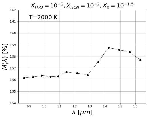
To demonstrate this, here we shall consider a more complex example motivated by the available data from the Hubble Space Telescope Wide Field Camera 3 (WFC3). Following previous studies in the literature, we shall consider $N_{bin}=13$ bins in the wavelength range $0.838-1.666\,{\mu}m$ (Kreidberg et al. 2015; Márquez-Neila et al. 2018). For our study here we shall choose $N_{bin}=3$ absorbers that are typically included in the analysis of transit spectra of hot Jupiters, namely water ($H_{2}O$), hydrogen cyanide ($HCN$) and gray clouds. The choice of chemical absorbers uniquely fixes the vector arrays $\vec{\xi}_{a}$ which are central to any inversion analysis. In our previous examples, we have been assuming constant $\vec{\xi}$’s, but in reality they depend on the temperature and (to a lesser extent) on the pressure. Therefore, to obtain reliable results from our inversion procedure, we need to account at least for the temperature dependence $\vec{\xi}_{a}(T)$. Figure 6 shows the wavelength dependence of the dimensionless absorption coefficients $\xi_{a}$ defined in (19), using the WFC3 binning for water (left panel) and HCN (right panel) in a temperature range starting from $T=500$ K and increasing by $\Delta T=250$ K. At the same time, for the gray clouds we shall continue to use a constant opacity vector $\vec{\xi}_{0}=\vec{u}$ as prescribed in (23).

Let us now define a study point with temperature $T=2000$ K and the following parameters for the absorbers

Figure 7 shows the generated transit spectrum for our study point (59). This is the starting point for our retrieval algorithm.

Next we calculate $\vec{r}$  from eq. (1) and decompose it into $\vec{r}_{\parallel}$ and $\vec{r}_{\perp}$ components, where for the latter, we use a system of $N_{bin}-1=12$ orthonormal basis vectors orthogonal to $\vec{u}$.

References

- Ardevol Martinez et al. (2022) Ardevol Martinez, F., Min, M., Kamp, I., & Palmer, P. I. 2022, arXiv e-prints, arXiv:2203.01236. https://arxiv.org/abs/2203.01236
- Barenblatt (1996) Barenblatt, G. I. 1996, Scaling, Self-similarity, and Intermediate Asymptotics: Dimensional Analysis and Intermediate Asymptotics, Cambridge Texts in Applied Mathematics (Cambridge University Press), doi: 10.1017/CBO9781107050242
- Barstow et al. (2020) Barstow, J. K., Changeat, Q., Garland, R., et al. 2020, MNRAS, 493, 4884, doi: 10.1093/mnras/staa548
- Barstow & Heng (2020) Barstow, J. K., & Heng, K. 2020, Space Sci. Rev., 216, 82, doi: 10.1007/s11214-020-00666-x
- Benneke & Seager (2012) Benneke, B., & Seager, S. 2012, ApJ, 753, 100, doi: 10.1088/0004-637X/753/2/100
- Bétrémieux & Swain (2017) Bétrémieux, Y., & Swain, M. R. 2017, MNRAS, 467, 2834, doi: 10.1093/mnras/stx257
- Blecic et al. (2021) Blecic, J., Harrington, J., Cubillos, P. E., et al. 2021, arXiv e-prints, arXiv:2104.12525. https://arxiv.org/abs/2104.12525
- Brown (2001) Brown, T. M. 2001, ApJ, 553, 1006, doi: 10.1086/320950
- Burrows et al. (2003) Burrows, A., Sudarsky, D., & Hubbard, W. B. 2003, ApJ, 594, 545, doi: 10.1086/376897
- Charbonneau et al. (2000) Charbonneau, D., Brown, T. M., Latham, D. W., & Mayor, M. 2000, ApJ, 529, L45, doi: 10.1086/312457
- Cobb et al. (2019) Cobb, A. D., Himes, M. D., Soboczenski, F., et al. 2019, AJ, 158, 33, doi: 10.3847/1538-3881/ab2390
- Cubillos et al. (2021) Cubillos, P. E., Harrington, J., Blecic, J., et al. 2021, arXiv e-prints, arXiv:2104.12524. https://arxiv.org/abs/2104.12524
- de Wit & Seager (2013) de Wit, J., & Seager, S. 2013, Science, 342, 1473, doi: 10.1126/science.1245450
- Fisher & Heng (2018) Fisher, C., & Heng, K. 2018, MNRAS, 481, 4698, doi: 10.1093/mnras/sty2550
- Fisher et al. (2020) Fisher, C., Hoeijmakers, H. J., Kitzmann, D., et al. 2020, AJ, 159, 192, doi: 10.3847/1538-3881/ab7a92
- Fortney (2005) Fortney, J. J. 2005, MNRAS, 364, 649, doi: 10.1111/j.1365-2966.2005.09587.x
- Griffith (2014) Griffith, C. A. 2014, Philosophical Transactions of the Royal Society of London Series A, 372, 20130086, doi: 10.1098/rsta.2013.0086
- Guzmán-Mesa et al. (2020) Guzmán-Mesa, A., Kitzmann, D., Fisher, C., et al. 2020, AJ, 160, 15, doi: 10.3847/1538-3881/ab9176
- Hanel et al. (2003) Hanel, R. A., Conrath, B. J., Jennings, D. E., & Samuelson, R. E. 2003, Exploration of the Solar System by Infrared Remote Sensing: Second Edition (Cambridge University Press)
- Harrington et al. (2021) Harrington, J., Himes, M. D., Cubillos, P. E., et al. 2021, arXiv e-prints, arXiv:2104.12522. https://arxiv.org/abs/2104.12522
- Heng (2019) Heng, K. 2019, MNRAS, 490, 3378, doi: 10.1093/mnras/stz2746
- Heng & Kitzmann (2017) Heng, K., & Kitzmann, D. 2017, MNRAS, 470, 2972, doi: 10.1093/mnras/stx1453
- Heng & Showman (2015) Heng, K., & Showman, A. P. 2015, Annual Review of Earth and Planetary Sciences, 43, 509, doi: 10.1146/annurev-earth-060614-105146
- Henry et al. (2000) Henry, G. W., Marcy, G. W., Butler, R. P., & Vogt, S. S. 2000, ApJ, 529, L41, doi: 10.1086/312458
- Himes et al. (2020a) Himes, M. D., Cobb, A. D., Wright, D. C., Scheffer, Z., & Harrington, J. 2020a, MARGE: Machine learning Algorithm for Radiative transfer of Generated Exoplanets. http://ascl.net/2003.010
- Himes et al. (2020b) Himes, M. D., Harrington, J., Cobb, A. D., et al. 2020b, arXiv e-prints, arXiv:2003.02430. https://arxiv.org/abs/2003.02430
- Himes et al. (2020c) Himes, M. D., Cobb, A. D., Soboczenski, F., et al. 2020c, in American Astronomical Society Meeting Abstracts, Vol. 235, American Astronomical Society Meeting Abstracts #235, 343.01
- Hubbard et al. (2001) Hubbard, W. B., Fortney, J. J., Lunine, J. I., et al. 2001, ApJ, 560, 413, doi: 10.1086/322490
- Hunter (2007) Hunter, J. D. 2007, Comput. Sci. Eng., 9, 90, doi: 10.1109/MCSE.2007.55
- Inc. (2015) Inc., P. T. 2015, Collaborative data science, Montreal, QC: Plotly Technologies Inc. https://plot.ly
- Kitzmann et al. (2020) Kitzmann, D., Heng, K., Oreshenko, M., et al. 2020, ApJ, 890, 174, doi: 10.3847/1538-4357/ab6d71
- Kluyver et al. (2016) Kluyver, T., Ragan-Kelley, B., Pérez, F., et al. 2016, in Positioning and Power in Academic Publishing: Players, Agents and Agendas, ed. F. Loizides & B. Scmidt (IOS Press), 87–90. https://eprints.soton.ac.uk/403913/
- Konar et al. (2010) Konar, P., Kong, K., Matchev, K. T., & Park, M. 2010, Phys. Rev. Lett., 105, 051802, doi: 10.1103/PhysRevLett.105.051802
- Kreidberg et al. (2015) Kreidberg, L., Line, M. R., Bean, J. L., et al. 2015, ApJ, 814, 66, doi: 10.1088/0004-637X/814/1/66
- Langhaar (1951) Langhaar, H. L. 1951, Dimensional Analysis and Theory of Models (Wiley)
- Madhusudhan (2019) Madhusudhan, N. 2019, ARA&A, 57, 617, doi: 10.1146/annurev-astro-081817-051846
- Márquez-Neila et al. (2018) Márquez-Neila, P., Fisher, C., Sznitman, R., & Heng, K. 2018, Nature Astronomy, 2, 719, doi: 10.1038/s41550-018-0504-2
- Matchev et al. (2021) Matchev, K. T., Matcheva, K., & Roman, A. 2021, arXiv e-prints, arXiv:2112.11600. https://arxiv.org/abs/2112.11600
- Matchev et al. (2022) —. 2022, arXiv e-prints, arXiv:2201.02696. https://arxiv.org/abs/2201.02696
- Matchev et al. (2020) Matchev, K. T., Roman, A., & Shyamsundar, P. 2020, SciPost. https://arxiv.org/abs/2002.06307
- Nixon & Madhusudhan (2020) Nixon, M. C., & Madhusudhan, N. 2020, MNRAS, 496, 269, doi: 10.1093/mnras/staa1150
- Oreshenko et al. (2020) Oreshenko, M., Kitzmann, D., Márquez-Neila, P., et al. 2020, AJ, 159, 6, doi: 10.3847/1538-3881/ab5955
- Perryman (2018) Perryman, M. 2018, The Exoplanet Handbook (Cambridge University Press)
- Schneider (1994) Schneider, J. 1994, Ap&SS, 212, 321, doi: 10.1007/BF00984535
- Seager & Sasselov (2000) Seager, S., & Sasselov, D. D. 2000, ApJ, 537, 916, doi: 10.1086/309088
- Vahidinia et al. (2014) Vahidinia, S., Cuzzi, J. N., Marley, M., & Fortney, J. 2014, ApJ, 789, L11, doi: 10.1088/2041-8205/789/1/L11
- van der Walt et al. (2011) van der Walt, S., Colbert, S. C., & Varoquaux, G. 2011, Computing in Science Engineering, 13, 22, doi: 10.1109/MCSE.2011.37
- Virtanen et al. (2020) Virtanen, P., Gommers, R., Oliphant, T. E., et al. 2020, Nature Methods, 17, 261, doi: 10.1038/s41592-019-0686-2
- Welbanks & Madhusudhan (2019) Welbanks, L., & Madhusudhan, N. 2019, AJ, 157, 206, doi: 10.3847/1538-3881/ab14de
- Welbanks & Madhusudhan (2021a) —. 2021a, ApJ, 913, 114, doi: 10.3847/1538-4357/abee94
- Welbanks & Madhusudhan (2021b) —. 2021b, On Atmospheric Retrievals of Exoplanets with Inhomogeneous Terminators. https://arxiv.org/abs/2112.09125
- Wright (2018) Wright, J. T. 2018, in Handbook of Exoplanets, ed. H. J. Deeg & J. A. Belmonte (Springer), 4, doi: 10.1007/978-3-319-55333-7_4
- Yip et al. (2021) Yip, K. H., Changeat, Q., Nikolaou, N., et al. 2021, AJ, 162, 195, doi: 10.3847/1538-3881/ac1744
- Zingales & Waldmann (2018) Zingales, T., & Waldmann, I. P. 2018, AJ, 156, 268, doi: 10.3847/1538-3881/aae77c