Safety-Aware and Data-Driven Predictive Control for Connected Automated Vehicles at a Mixed Traffic Signalized IntersectionfootnoteinfoThis research was supported by ARPAE’s NEXTCAR program under the award number DE-AR0000796.
Abstract
A typical urban signalized intersection poses significant modeling and control challenges in a mixed traffic environment consisting of connected automated vehicles (CAVs) and human-driven vehicles (HDVs). In this paper, we address the problem of deriving safe trajectories for CAVs in a mixed traffic environment that prioritizes rear-end collision avoidance when the preceding HDVs approach the yellow and red signal phases of the intersection. We present a predictive control framework that employs a recursive least squares algorithm to approximate in real time the driving behavior of the preceding HDVs and then uses this approximation to derive safety-aware trajectory in a finite horizon. We validate the effectiveness of our proposed framework through numerical simulation and analyze the robustness of the control framework.
keywords
Connected automated vehicles; predictive control; data-driven parameter estimation; vehicle safety; mixed traffic environment., ,
1 Introduction
Optimal coordination of connected automated vehicles (CAVs) can improve network performance, e.g., fuel economy, traffic throughput, at traffic scenarios such as urban intersections, see Talebpour and Mahmassani 2016. In recent efforts, a decentralized optimal control framework has been established for real-time coordination of CAVs traveling through signal-free automated intersections, see Malikopoulos et al. 2021; Chalaki and Malikopoulos 2021; Mahbub and Malikopoulos 2021; Kumaravel et al. 2021. However, these approaches have been developed based on the strict assumption of 100% CAV penetration rate which is currently not realizable; see Alessandrini et al. 2015.
CAVs must be able to safely co-exist with human-driven vehicles (HDVs) resulting in a mixed traffic environment, which pose significant modeling and control challenges due to the stochastic nature of human-driving behavior. Furthermore, the use of conventional traffic lights is still the most prevalent way of traffic control at urban intersections that adds an extra layer of complexity in modeling the HDV behavior due to the presence of the zone of yellow light dilemma; see Zhang et al. 2014. Thus, the need for an efficient CAV control framework considering the inclusion and interaction of HDVs approaching the signalized intersections is essential to provide safety assurance under unknown HDV behavior.
Several research efforts have adopted adaptive cruise control (ACC) for automated vehicles in a mixed traffic environment to tackle the HDV behavior and ensure rear-end collision avoidance; see Jiang et al. 2007; Yuan et al. 2009. Lu et al. 2019 considered a variation of the car-following model to design an eco ACC controller. However, ACC controllers using car-following models such as the intelligent driver model (IDM) (Treiber and Kesting 2013) do not always perform well since they can have stability implications leading to rear-end collision; see Milanés and Shladover 2014. Milanés et al. 2013 proposed a cooperative adaptive cruise controller where the control parameters are derived using system identification on real-world experimental data. However, such control parameters cannot capture the instantaneous changes in HDV behavior. Naus et al. 2010 proposed an explicit model predictive control (MPC) ACC controller that employs a prediction model with a constant speed assumption of the preceding vehicle and does not consider the complex car-following dynamics of the human driver. Dollar et al. 2021 utilized an IDM model to identify offline the human driving styles in a car-following scenario and developed an MPC-based cruise control for a CAV. Jin and Orosz 2018 proposed an optimal cruise control design in which feedback gains and driver reaction time of HDVs were estimated in real time by a sweeping least square method.
In this paper, we consider the problem related to controlling a CAV while approaching a signalized intersection in the presence of multiple preceding HDVs with unknown driving behavior. To generate safe and optimal control actions for the CAV, we propose a data-driven predictive control framework that takes into account the future trajectories of the HDVs to ensure that the collision does not take place over a finite-time horizon. The control framework is then implemented in a receding horizon manner for robustness against stochastic driving behavior of HDVs. The constant time headway relative velocity (CTH-RV) model and the recursive least squares (RLS) algorithm are utilized to estimate the HDV’s driving behavior given the data collected online. We evaluate the efficiency of the proposed method by numerical simulations that employ a nonlinear car-following model to replicate the human drivers.
The remainder of the paper is organized as follows. In Section 2, we present the modeling framework and formulate the problem. In Section 3, we provide a detailed exposition of the safety-aware and data-driven predictive control framework with real-time behavior estimation. In Section 4, we evaluate the effectiveness of the proposed approach in a simulation environment. Finally, we draw conclusions and discuss the future research directions in Section 5.
2 Problem Formulation
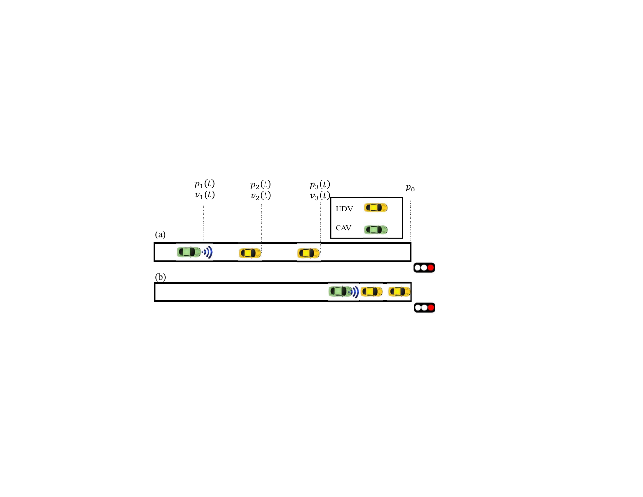
We consider multiple HDVs followed by a CAV traveling on a single-lane road and approaching an urban signalized intersection with a red (or yellow then red) traffic signal phase (Fig. 1). Note that, the general idea of our formulation can be extended to different cases such as yield/stop traffic sign, downstream traffic congestion, and pedestrian crossing, where the preceding HDVs’ motion can change abruptly to come to a full stop. Next, to facilitate our exposition we provide the following definitions.
Definition 1
Suppose that the red signal phase is active at some time instant . The set of the vehicles approaching the intersection at is , where is the total number of vehicles under consideration. Here, the vehicles are assigned integer indices by the order of their respective distances from some fixed stopping position located downstream near the signal head. The indices represent the HDVs followed by the CAV denoted by the index .
Definition 2
The set of HDVs at time instant is .
When the red signal phase is active at some time instant , the HDV- in must stop behind the position . The objective of the CAV- is to derive an optimal trajectory to stop behind HDV- such that no rear-end collision takes place.
Remark 3
In our formulation, we require that the set of HDVs is non-empty at time instant when the red signal phase of the intersection is active. If is empty, then the problem of avoiding rear-end collision becomes redundant.
2.1 Communication Topology
The CAV- is retrofitted with appropriate sensors and communication devices to estimate in real time the state information of the preceding HDVs in through vehicle-to-everything communication protocol and intelligent roadside units; see Duan and Yang 2021. We refer to the unidirectional flow of information from the preceding HDVs in to the trailing CAV- as the multi-predecessor communication topology.
We impose the following assumption.
Assumption 4
Communication to and from the CAV occurs without any delays and errors.
Assumption 4 may be strong, but it is relatively straightforward to relax it as long as the noise in the measurements and/or delays is bounded.
In contrast, the trajectory of each HDV in is solely dictated by the perception of the state information of the immediate preceding HDV in . For the leading vehicle HDV- that does not have a preceding vehicle, its driving actions depend on the relative distance to the stopping point.
2.2 Vehicle Dynamics and Constraints
We consider the following discrete-time model with a sampling time to represent the dynamics of each vehicle ,
| (1a) | ||||
| (1b) | ||||
where , , and denote the position, speed and control input (acceleration/deceleration) of each vehicle in . The sets , , and , are complete and totally bounded subsets of . Note that in the discrete-time dynamics model (1), we assume that the control input of each vehicle in remains constant in the time period of length between time instants and , which is different to some previous approaches that assume constant speed between time instants and ; see Naus et al. 2010; Kianfar et al. 2012.
To ensure that the control input and vehicle speed are within a given admissible range, the following constraints are imposed,
| (2a) | ||||
| (2b) | ||||
where , are the maximum braking and acceleration, respectively, of each vehicle in , and , are the minimum and maximum speed limits, respectively.
The control input of each vehicle in (1) can take different forms based on the consideration of connectivity and automation. For CAV- in , we consider a switching control framework based on the following cases: if at time instant (Remark 3) (a) is empty, then CAV- derives its control input by using its default adaptive cruise controller (see Milanés and Shladover 2014), (b) if is not empty, then CAV- derives and implements the control input using the proposed control framework discussed in Section 3.
For each HDV , however, we consider a car-following model to represent the predecessor-follower coupled dynamics (Fig. 1) with its preceding vehicle that has the following generic structure
| (3) |
where represents the behavioral function of the car-following model of vehicle , and and denote the headway and approach rate of vehicle with respect to its preceding vehicle , respectively. We consider two edge cases that may arise from the above definitions: (a) if there is no vehicle preceding vehicle within a certain look-ahead distance , then we consider and , and (b) if there is an obstruction/red signal phase immediately ahead of vehicle at a distance , then and . There are several car-following models reported in the literature that can emulate a varied class of human driving behavior; see Weng and Wu 2001.
The parameters of a car-following model can be recovered from historical data using offline identification methods; see Treiber and Kesting 2013. However, since the historical data might not be available and the human driving behavior usually changes over time, offline identification methods do not work well in practice. As a result, in our proposed framework, we consider that the CAV does not have full prior knowledge of the behavioral function of the preceding HDVs. Instead, the CAV assumes a specific type of car-following model for the HDV, then estimates the model parameters for each HDV online using real-time collected data. A method for estimating car-following model parameters of the HDVs is given in Section 3.1.
To capture the car-following characteristics of the preceding HDV-’s dynamics from the CAV-’s control point of view, we define additional states as
| (4a) | ||||
| (4b) | ||||
To introduce the rear-end collision avoidance constraint, we first use the following definition of dynamic safe following headway .
Definition 5
The dynamic safe following headway between two consecutive vehicles is
| (5) |
where denotes a desired time headway that each vehicle maintains while following the preceding vehicle, and is the standstill distance denoting the minimum bumper-to-bumper gap at stop.
The rear-end collision avoidance constraint between CAV- and its immediately preceding HDV- can thus be written as
| (6) |
We now formalize the main objective of the CAV- control framework.
Problem 6
Given the multi-predecessor communication topology (Section 2.1), the main objective of CAV- is to derive its optimal control input such that CAV- adapts to its preceding HDV’s driving behavior in real time and drives the states and to their respective reference states with minimum control effort satisfying the state, control and safety constraints in (2)-(6).
3 Control Framework
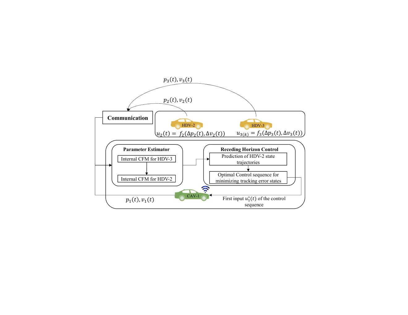
In our approach, we adopt a receding horizon predictive control framework with multi-predecessor communication topology and data-driven estimation of HDVs’ car-following parameters for state prediction to address Problem 6, as shown in Figure 2. In the receding horizon control, the optimal control input at the current time step is obtained by solving a predictive control problem with a horizon while only the first element of the obtained control input sequence is implemented. Afterward, the horizon moves forward one step, and the above process is repeated until a final horizon is reached; see Borrelli et al. 2017. Note that, the prediction horizon is usually selected empirically to best accommodate the control performance and computational requirement. The essential steps of the proposed framework are outlined as follows.
- 1.
Data-driven parameter estimation: At each time instant , the current states of each preceding HDV in is communicated to CAV-. Since the exact car-following model of each HDV in is unknown to CAV-, it considers a specific type of car-following model to represent the driving behavior of each HDV, and estimates the parameters of the car-following model for each HDV online.
- 2.
Predictive control problem: CAV- then uses the estimated car-following model from Step 1 to predict the future state trajectories of the immediately preceding HDV- and derives its own optimal control input sequence using the receding horizon control framework discussed above. Finally, CAV- implements only the first control input .
In what follows, we provide a detailed exposition of the steps discussed above.
3.1 Online Car-following Model Parameter Estimation
In this section, we use a recursive least-squared formulation (Ljung and Söderström 1983) to estimate the parameters of the internal car-following model residing in CAV-’s mainframe to represent the driving behavior of each of the preceding HDVs. To this end, we consider the CTH-RV model (Wang et al. 2020)
| (7) |
where the model parameters and are the control gains on the constant time headway and the approach rate, and is the desired safe time headway for each HDV in , respectively. We employ the linear CTH-RV model instead of other complex nonlinear models so that the resulting control problem presented in the next section is thus convex and can be solved efficiently in real-time. Moreover, it is also observed that the CTH-RV model is highly comparable to other nonlinear car-following models in terms of data fitting (Gunter et al. 2019).
Suppose that we measure the speed , headway gap and approach rate for each preceding HDV in with sampling rate . We recast (7) as
| (8) |
where , and are the parameters that can be estimated using the RLS algorithm. The original model parameters and are then uniquely determined from as long as . Next, we can write (8) in matrix form as
| (9) |
where is the regressor vector and is the parameter vector. We can estimate using the following recursive least squares algorithm as follows (Ljung and Söderström 1983)
| (10a) | ||||
| (10b) | ||||
| (10c) | ||||
| (10d) | ||||
Here, is the forgetting factor that assigns a higher weight to the recently collected data points and discounts older measurements, and denotes the estimate of the parameter vector at time instant , which is updated recursively as new data becomes available. In what follows, we introduce the predictive control problem that is needed to be solved.
3.2 Predictive Control Problem
The main objective of the predictive controller of the CAV is to (a) drive the position tracking state to a reference , (b) drive the speed tracking state to zero, and (c) minimize CAV-’s control input . To this end, the receding horizon controller generates the predictive states for at each time instant for a predictive horizon using the state definitions in (4), vehicle dynamics in (1) and internal car-following models of the HDVs in (7) approximated in the previous section. Then the control input sequence is derived such that the predictive states are driven to their respective reference states. The predictive control problem thus can be written as
| (11) | ||||
where the predictive reference state can be computed using the relation and the dynamics model in (1) and (4), and are the weights on the reference tracking of the headway , speed deviation , and the CAV-’s control input , respectively.
The predictive control problem in (11) can be transformed into a standard constrained quadratic programming problem and solved using commercially available solvers; see Andersson et al. 2019a. At each discrete time instant , the optimal control sequence is computed by solving (11) and only the first control input is applied. Then the system moves to the next time instant and the process is repeated until a final time horizon is reached.
Remark 7
While implementing the above control framework, if any of the preceding HDVs leaves the current lane or passes the intersection at any time instant , we simply update the sets and starting from the next time instant , where the control problem (11) is again solved with the updated information.
4 Simulation and Result
This section validates the performance of the proposed safety-aware data-driven predictive control by numerical simulations at a mixed-traffic signalized intersection.
4.1 Simulation Setup
In the simulations, we utilize a nonlinear car-following model namely the optimal velocity model (OVM) to generate the driving actions of simulated human drivers (Bando et al. 1995). The car-following OVM is given as
| (12) |
The parameters of the OVM for each HDV include the driver’s sensitivity coefficients and , and the desired speed . These parameters for the simulated HDVs are assumed to be different to each other and chosen by random perturbations up to 20% around the following nominal values: , , , , . The parameters and weights in the predictive control framework used for the simulations are given in Table 1. The RLS-based estimators are initialized with the following values: and where is the identity matrix, while the forgetting factor is chosen as . The impact of on RLS algorithm is investigated in detail by Vahidi et al. 2005 and thus, omitted here. Python is used in the simulations in which the constrained optimal control problem is formulated by CasADi framework; see Andersson et al. 2019b, and solved by the built-in qpOASES solver.
| Parameters | Value | Parameters | Value |
|---|---|---|---|
| 50 | |||
| 1 | 0.1 | ||
| 1 |
4.2 Results and Discussions
The results for a numerical simulation involving a CAV and 2 preceding HDVs are illustrated in Fig. 3, in which the longitudinal positions, speeds, and headways of all the vehicles are given in Figures 3(a), 3(b) and 3(c), respectively. Note that the position by which the vehicles must stop is , and for the leading HDV, the headway is computed as the relative distance to the stopping point. As can be seen from Figures 3(a)-3(c), the simulated HDVs slow down and then stop while approaching the signalized intersection. Given the behavior of the HDVs, the proposed control framework can perform safe and comfortable braking for the CAV without violating any of the state, input, and safety constraints.
Moreover, to assess the scalability of the proposed control framework to the number of preceding vehicles, we conduct three other simulations for the scenarios with 4, 5, and 6 vehicles (3, 4, and 5 HDVs, respectively) and illustrate the vehicle trajectories in Fig. 4. These results verify that the proposed control framework works effectively with different numbers of preceding vehicles.
Finally, the estimated parameters in the CTH-RV car-following model for the HDV-2 are depicted in Fig. 5. As more real-time data are added to update the estimations, the car-following parameters stabilize to the set of values that accurately describes the driving behavior of the HDVs. Therefore, using the linear CTH-RV model and online RLS technique, we can approximate a nonlinear car-following model and use this estimation to predict the future states of the HDVs.
5 Concluding Remarks
In this paper, we addressed the problem of a CAV traveling in a mixed traffic environment and approaching a signalized intersection. A data-driven predictive control framework was developed in which the car-following behavior of HDVs ahead of the CAV is modeled by the CTH-RV model with online estimated parameters through the RLS algorithm. In the proposed framework, by utilizing data-driven car-following models, the CAVs can predict the future behavior of the HDVs and then derive their optimal safety-aware trajectory in a finite horizon. The proposed control framework was validated by numerical simulations with multiple preceding HDVs showing that the generated control actions can ensure safe braking for the CAVs. A direction for future research should focus on extending this framework to consider multi-lane traffic intersections with lane changing behavior of the HDVs.
References
- Alessandrini et al. (2015) Alessandrini, A., Campagna, A., Delle Site, P., Filippi, F., and Persia, L. (2015). Automated vehicles and the rethinking of mobility and cities. Transportation Research Procedia, 5, 145–160.
- Andersson et al. (2019a) Andersson, J.A.E., Gillis, J., Horn, G., Rawlings, J.B., and Diehl, M. (2019a). CasADi – A software framework for nonlinear optimization and optimal control. Mathematical Programming Computation, 11(1), 1–36.
- Andersson et al. (2019b) Andersson, J.A., Gillis, J., Horn, G., Rawlings, J.B., and Diehl, M. (2019b). Casadi: a software framework for nonlinear optimization and optimal control. Mathematical Programming Computation, 11(1), 1–36.
- Bando et al. (1995) Bando, M., Hasebe, K., Nakayama, A., Shibata, A., and Sugiyama, Y. (1995). Dynamical model of traffic congestion and numerical simulation. Physical review E, 51(2), 1035.
- Borrelli et al. (2017) Borrelli, F., Bemporad, A., and Morari, M. (2017). Predictive control for linear and hybrid systems. Cambridge University Press.
- Chalaki and Malikopoulos (2021) Chalaki, B. and Malikopoulos, A.A. (2021). Time-optimal coordination for connected and automated vehicles at adjacent intersections. IEEE Transactions on Intelligent Transportation Systems, 1–16.
- Dollar et al. (2021) Dollar, R.A., Molnár, T.G., Vahidi, A., and Orosz, G. (2021). Mpc-based connected cruise control with multiple human predecessors. In 2021 American Control Conference (ACC), 405–411. IEEE.
- Duan and Yang (2021) Duan, Z. and Yang, Z. (2021). Smart city traffic intersection: Impact of video quality and scene complexity on precision and inference. In in Proc. 19th IEEE Int. Conf. on Smart City, 2021.
- Gunter et al. (2019) Gunter, G., Stern, R., and Work, D.B. (2019). Modeling adaptive cruise control vehicles from experimental data: model comparison. In 2019 IEEE Intelligent Transportation Systems Conference (ITSC), 3049–3054. IEEE.
- Jiang et al. (2007) Jiang, R., Hu, M.B., Jia, B., Wang, R., and Wu, Q.S. (2007). Phase transition in a mixture of adaptive cruise control vehicles and manual vehicles. The European Physical Journal B, 58(2), 197–206.
- Jin and Orosz (2018) Jin, I.G. and Orosz, G. (2018). Connected cruise control among human-driven vehicles: Experiment-based parameter estimation and optimal control design. Transportation research part C: emerging technologies, 95, 445–459.
- Kianfar et al. (2012) Kianfar, R., Augusto, B., Ebadighajari, A., Hakeem, U., Nilsson, J., Raza, A., Tabar, R.S., Irukulapati, N.V., Englund, C., Falcone, P., et al. (2012). Design and experimental validation of a cooperative driving system in the grand cooperative driving challenge. IEEE transactions on intelligent transportation systems, 13(3), 994–1007.
- Kumaravel et al. (2021) Kumaravel, S., Malikopoulos, A.A., and Ayyagari, R. (2021). Decentralized cooperative merging of platoons of connected and automated vehicles at highway on-ramps. In 2021 American Control Conference (ACC), 2055–2060.
- Ljung and Söderström (1983) Ljung, L. and Söderström, T. (1983). Theory and practice of recursive identification. MIT press.
- Lu et al. (2019) Lu, C., Dong, J., Hu, L., and Liu, C. (2019). An ecological adaptive cruise control for mixed traffic and its stabilization effect. IEEE Access, 7, 81246–81256.
- Mahbub and Malikopoulos (2021) Mahbub, A.M.I. and Malikopoulos, A.A. (2021). Conditions to Provable System-Wide Optimal Coordination of Connected and Automated Vehicles. Automatica, 131(109751).
- Malikopoulos et al. (2021) Malikopoulos, A.A., Beaver, L.E., and Chremos, I.V. (2021). Optimal time trajectory and coordination for connected and automated vehicles. Automatica, 125(109469).
- Milanés and Shladover (2014) Milanés, V. and Shladover, S.E. (2014). Modeling cooperative and autonomous adaptive cruise control dynamic responses using experimental data. Transportation Research Part C: Emerging Technologies, 48, 285–300.
- Milanés et al. (2013) Milanés, V., Shladover, S.E., Spring, J., Nowakowski, C., Kawazoe, H., and Nakamura, M. (2013). Cooperative adaptive cruise control in real traffic situations. IEEE Transactions on intelligent transportation systems, 15(1), 296–305.
- Naus et al. (2010) Naus, G.J., Ploeg, J., Van de Molengraft, M., Heemels, W., and Steinbuch, M. (2010). A model predictive control approach to design a parameterized adaptive cruise control. In Automotive Model Predictive Control, 273–284. Springer.
- Talebpour and Mahmassani (2016) Talebpour, A. and Mahmassani, H.S. (2016). Influence of connected and autonomous vehicles on traffic flow stability and throughput. Transportation Research Part C: Emerging Technologies, 71, 143–163.
- Treiber and Kesting (2013) Treiber, M. and Kesting, A. (2013). Traffic flow dynamics. Traffic Flow Dynamics: Data, Models and Simulation, Springer-Verlag Berlin Heidelberg.
- Vahidi et al. (2005) Vahidi, A., Stefanopoulou, A., and Peng, H. (2005). Recursive least squares with forgetting for online estimation of vehicle mass and road grade: theory and experiments. Vehicle System Dynamics, 43(1), 31–55.
- Wang et al. (2020) Wang, Y., Gunter, G., Nice, M., Delle Monache, M.L., and Work, D.B. (2020). Online parameter estimation methods for adaptive cruise control systems. IEEE Transactions on Intelligent Vehicles, 6(2), 288–298.
- Weng and Wu (2001) Weng, Y. and Wu, T. (2001). Car-following model of vehicular traffic. In 2001 International Conferences on Info-Tech and Info-Net, volume 4, 101–106 vol.4.
- Yuan et al. (2009) Yuan, Y.M., Jiang, R., Hu, M.B., Wu, Q.S., and Wang, R. (2009). Traffic flow characteristics in a mixed traffic system consisting of acc vehicles and manual vehicles: A hybrid modelling approach. Physica A: Statistical Mechanics and its Applications, 388(12), 2483–2491.
- Zhang et al. (2014) Zhang, Y., Fu, C., and Hu, L. (2014). Yellow light dilemma zone researches: a review. Journal of traffic and transportation engineering (English edition), 1(5), 338–352.