Controlling the flexibility of non-Gaussian processes through shrinkage priors

Autoregressive processes with GH innovating terms are discussed in Ghasami et al. 2020 and can model extreme market movements not captured by the Gaussian model (Dhull and Kumar 2021). Bibby and Sørensen 2003 presented more sophisticated models for financial time series, namely stochastic processes whose marginal distributions or the distributions of increments (or both) are generalized hyperbolic, including classical diffusion processes and stochastic volatility models (Barndorff-Nielsen 1997; Barndorff-Nielsen and Shephard 2001; Barndorff-Nielsen and Shephard 2002). The empirical distributions of the log-returns of financial time series are too heavy for satisfactory fitting by normal densities, and the GH distribution can better capture the stylized features of financial data.

In the field of spatial statistics, Bolin 2014 provided a class of non-Gaussian random fields with Matérn covariance function, constructed as solutions to stochastic partial differential equations (SPDEs) driven by Generalized Hyperbolic noise. The previous models were applied in the context of geostatistics (Wallin and Bolin 2015), joint modeling of multivariate random fields (Bolin and Wallin 2020), and to model continuously repeated measurement data collected longitudinally (Asar et al. 2020), where the non-Gaussian models led to improved predictive power in datasets where there were sharp spikes or jumps in the observed data that the Gaussian models oversmoothed.

The aforementioned papers performed parameter estimation of non-Gaussian models via likelihood maximization techniques or by the method of moments. Bayesian estimation was carried out for the same geostatistical framework of Wallin and Bolin 2015 by Walder and Hanks 2020. A Bayesian framework has also been considered for stochastic volatility models (Xie and Shen 2021; Nakajima and Omori 2012), for a vector of autoregressive processes (Karlsson et al. 2021), and GARCH models (Deschamps 2012), and all previously cited papers utilized the generalized hyperbolic skew Student’s $t$ (GHSST) distribution for the driving noise. In the same papers, a gamma prior was chosen for the leptokurtosis parameter and a normal prior for the skewness parameter of the GHSST distribution. There was no principled motivation for the use of these priors other than mathematical or computational convenience, and the gamma prior places 0 mass at the base Gaussian model, thus forcing overfitting of the data (Simpson et al. 2017).

Here we present the layout of the paper and highlight what are its main contributions to the literature on non-Gaussian processes from a Bayesian perspective. We find in the current literature challenges when it comes to model interpretability, sensible prior selection, and ease of implementation which we address next.

Parameterization and interpretability: Parameterizations of the NIG and GAL distributions involve 4 parameters that are used to regulate the mean, variance, skewness, and kurtosis of the distribution. However, the parameterizations are not themselves property-based leading to a difficult interpretation of the parameters. This also presents a difficulty when constructing priors for the parameters, since, for instance, the mean and variance will depend not only on the location and scale parameter but also on the other parameters. In section 2 we provide a property-based parameterization of the NIG and GAL distributions that preserves the mean and covariance structure of the Gaussian model.

Priors that avoid overfitting and lead to a robust estimation: Fig. 1 shows posterior means of the leptokurtosis parameter $\eta$ of the NIG distribution when fitting i.i.d. standard Gaussian data. These were obtained by numerical integration of the unnormalized $\pi(\eta|\mathbf{y})\propto\prod_{i}^{n}\pi_{\text{NIG}}(y_{i}|\eta)\pi(\eta)$, where $\pi_{\text{NIG}}$ is the probability density function (PDF) of the standardized and symmetric NIG distribution of subsection 2.1. The Gaussian and Cauchy distributions are limit distributions when $\eta\to 0$ and $\eta\to\infty$, respectively. If we use a uniform prior for small samples the results suggest the necessity of a non-Gaussian model when the simpler Gaussian model should be the preferred one. We should prefer the Gaussian model not only for parsimony’s sake but also because for Gaussian simulated data, the expected predictive performance will be the highest for the Gaussian model if a strictly proper scoring rule is used to evaluate the predictive accuracy (Gneiting and Raftery 2007). The tendency to overestimate the degree of non-Gaussianity in the data is more severe when a non-Gaussian model is added as a latent component in a hierarchical model and can be prevalent even for samples sizes of 500, as our simulation study in section 5 shows. This issue motivates an inferential framework that contracts non-Gaussian models towards Gaussianity in the absence of sufficient evidence of non-trivial leptokurtosis or asymmetry. In section 3 we construct prior distributions for the skewness and leptokurtosis parameters of the NIG and GAL distribution based on the penalized complexity (PC) priors principled approach of Simpson et al. 2017.

Many models, one framework: We presented in the previous subsection a wide range of models, defined in discrete or continuous space, for time series or spatial data. We unify these models into a single generic class, which we examine in section 2. We also offer in section 4 a set functions for the $Stan$ platform (Stan Development Team 2020) that allow a straightforward implementation of these models.

Bayesian analysis: A simulation study is conducted to compare the PC priors with other priors choices in section 5, and the developed methods are applied to two spatial datasets in section 6. The analysis showed that the PC priors achieve the sought contraction towards the Gaussian model when there is not enough convincing evidence in the data of non-Gaussianity and lead to more robust estimation.

Finally, section 7 contains a summary and discussion of future work and possible extensions.

In the previous parameterization $(\lambda,\alpha,\beta,\delta,\mu)$, the location ($\mu$) and scale ($\delta$) parameters do not correspond to the mean and standard deviation of the distribution. For the NIG distribution setting $\mu=0$ and $\delta=1$ leads to $E[\Lambda]=\beta/(-\alpha^{2}+\beta^{2})$ and $V[\Lambda]=\alpha^{2}/(\alpha^{2}-\beta^{2})^{3/2}$, and so the mean and variance depend on the degree of asymmetry and leptokurtosis of the distribution. There are alternative parameterizations of the GH distribution in the literature (Paolella 2007; Prause et al. 1999), including location-scale invariant ones, but these continue to not be property-based.

As in Niekerk and Rue 2021 we posit that when constructing priors the mean and the standard deviation should be fixed, instead of location and scale parameters. This not only eases interpretation but also allows assigning the priors for the mean and scale of the Gaussian model in non-Gaussian models, which is very convenient when implementing these non-Gaussian models in practice (otherwise reasonable priors for the location and scale would have to depended on $\alpha$ and $\beta$). Table 1 shows the conversion between the standardized parameterization and the more conventional one in eq. (1), along with some relevant moments (consider for now $h=1$). The variance-mean mixture representation belonging to this parameterization is

$\displaystyle\Lambda|V$

$\displaystyle\sim\text{N}\left(\frac{1}{\sqrt{1+\eta\zeta^{2}}}\zeta(V-h),\ \ \frac{1}{1+\eta\zeta^{2}}V\right),V{\sim}\begin{cases}\text{IG}(1,\eta^{-1})&\text{(NIG)}\\ \text{Gamma}(\eta^{-1},\eta^{-1})&\text{(GAL).}\end{cases}$

(2)

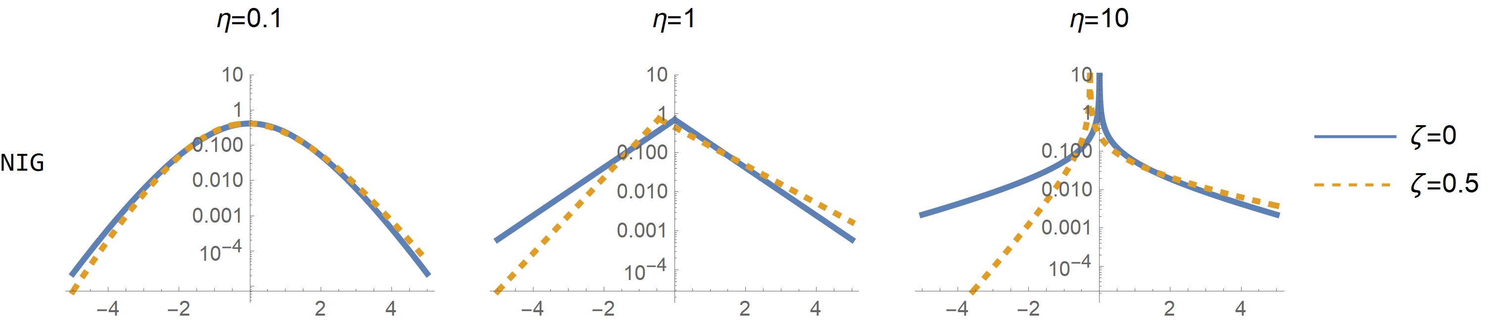
A location and scale parameter can be added by the usual transformation $m+\sigma\Lambda$, and the mean and variance will be $m$ and $\sigma^{2}$, regardless of the other parameters’ value. The parameter $\eta$ is related to the degree of non-Gaussianity since $\Lambda$ converges to a Gaussian random variable when $\eta\to 0$, and as we increase $\eta$, the excess kurtosis increase. The parameter $\zeta$ is related to the asymmetry of the random variable since $\Lambda$ is symmetric when $\zeta=0$, and when $\zeta>0$, it is skewed to the right. Here and henceforth, we will make use of the notions of “base model”, “flexible model” and “flexibility parameter” defined in Simpson et al. 2017. We see the non-Gaussian model parameterized by $(\eta,\zeta)$ as a flexible extension of the base Gaussian model since it contains the Gaussian model as a special case (when $\eta=\zeta=0$) and deviations from the Gaussian model are quantified by the parameters $\eta$ and $\zeta$ to which we refer as flexibility parameters. The densities of the NIG and GAL distributions with the previous parameterization are displayed in Fig. 2. We observe that the larger the value of $\eta$, the larger the asymmetry induced by the same value of the parameter $\zeta$.

There is still some confounding between $\eta$ and $\zeta$ in the standardized parameterization since the excess kurtosis increases with $\zeta$, so a prior for $\eta$ derived for a symmetric model may not shrink the models towards Gaussianity as much as we anticipate if the data is asymmetric. Thus, we need to associate $\eta$ with some interpretable model property and then guarantee that the property is invariant with the second flexibility parameter. This will also allow using the PC prior of $\eta$, which is derived in section 3 for the symmetric case, in asymmetric data.

We find the kurtosis to be hard to interpret (it is not clear what an increase in kurtosis of 1 means in practice) and so we prefer to associate $\eta$ with the likelihood of large events. For the NIG distribution this probability can be approximated by $P(|\Lambda|>x)\propto x^{-3/2}\exp(-\eta^{-1/2}\xi_{NIG}x)$ for large $x$ (Hammerstein 2016). The dependency of this probability with the skewness parameter $\zeta$ comes through the rate $\xi_{NIG}$:

$$\xi_{\text{NIG}}=1+\zeta^{2}\eta-|\zeta|\sqrt{\eta(1+\zeta^{2}\eta)},$$

which is equal to 1 in the symmetric case ($\zeta=0$). We require the probability $P(|\Lambda|>x)$ to be invariant with the skewness parameter, at least for large $x$. This can be achieved by the parameter transformations $\eta^{\star}=\eta\xi_{NIG}^{-2}$ and $\zeta^{\star}=\zeta\sqrt{\eta}$. The same transformation applies for the GAL distribution where one should take

$$\xi_{\text{GAL}}=\sqrt{1+\zeta^{2}\eta}(\sqrt{2+\zeta^{2}\eta}-|\zeta|\sqrt{\eta}).$$

We note that these transformations on the flexibility parameters do not affect the mean (0) and the variance (1) of the standardized parameterization. The quantity $\xi$ is also related to the excess kurtosis, namely $\text{EKurt}[\Lambda]\approx 9/\xi^{2}$, for both the NIG and GAL distributions. Therefore, by guaranteeing that $P(|\Lambda|>x)$ is invariant with $\zeta^{\star}$ for large $x$, we also guarantee that the kurtosis of the noise (and the process’ marginal distributions) remains approximately the same for different values of $\zeta^{\star}$, leading to a more orthogonal interpretation of the parameters.

Let $\mathbf{x}^{G}$ be a random vector that follows a multivariate Gaussian distribution with dimension $n$, mean $m$, and precision matrix $\mathbf{Q}=\sigma^{-2}\mathbf{\mathbf{D}}^{T}\mathbf{D}$. It can be expressed through

$$\mathbf{D}(\mathbf{x}^{G}-m)\overset{d}{=}\sigma\mathbf{Z},$$

(3)

where $\mathbf{Z}=[Z_{1},\dotsc,Z_{n}]^{T}$ is a vector of i.i.d. standard Gaussian variables. When $\mathbf{x}^{G}$ is derived from a process defined in continuous space, one usually has $Z_{i}\overset{ind.}{\sim}\text{N}(0,h_{i})$ for some predefined constant $h_{i}$ (for instance, the distance between locations in an autoregressive process), and so the precision matrix is $\mathbf{Q}=\sigma^{-2}\mathbf{D}^{T}\text{diag}(\mathbf{h})^{-1}\mathbf{D}$. The non-Gaussian extension for $\mathbf{x}$ consists in replacing the driving noise distribution:

$$\mathbf{D}(\mathbf{x}-m)\overset{d}{=}\sigma\mathbf{\Lambda},$$

(4)

where $\bm{\Lambda}=[\Lambda_{1},\dotsc,\Lambda_{n}]^{T}$ is a vector of independent and standardized NIG or GAL random variables that depend on parameters $\eta$ and $\zeta$. Using the parameterizations in subsections 2.1 and 2.2 for $\mathbf{\Lambda}$, the non-Gaussian random vector $\mathbf{x}$ has the same mean and covariance matrix as the Gaussian random vector $\mathbf{x}^{G}$ but with more flexible sample path properties and marginal distributions whose kurtosis and skewness are regulated by the flexibility parameters $\eta$ and $\zeta$. Appendix B contains more properties about non-Gaussian models defined via eq. (4). It is important to mention that these models are not uniquely specified by their covariance or precision matrices but through the matrix $\mathbf{D}$. In section 4 we show that many of the non-Gaussian models mentioned in the Introduction belong to the generic class of models defined by eq. (4).

A variance-mean mixture representation of the non-Gaussian random vector $\mathbf{x}$ is obtained by considering the random vector $\mathbf{V}=[V_{1},\dotsc,V_{n}]^{T}$ and the predefined vector $\mathbf{h}=[h_{1},\dotsc,h_{n}]^{T}$, containing the mixing distributions and some predefined constants, respectively. In the standardized parameterization it is:

$\displaystyle\begin{split}\mathbf{x}|\mathbf{V}&\sim\text{N}\left(m+\frac{\sigma}{\sqrt{1+\zeta^{2}\eta}}\zeta\mathbf{D}^{-1}(\mathbf{V}-\mathbf{h}),\frac{\sigma^{2}}{1+\zeta^{2}\eta}\mathbf{D}^{-1}\text{diag}(\mathbf{V})\mathbf{D}^{-T}\right),\\ V_{i}&\overset{ind.}{\sim}\begin{cases}\text{IG}(h_{i},\eta^{-1}h_{i}^{2})&\text{(NIG Noise)}\\ \text{Gamma}(h_{i}\eta^{-1},\eta^{-1})&\text{(GAL Noise).}\end{cases}\end{split}$

(5)

To broaden the applicability of the multivariate model $\mathbf{x}$ to data measured at irregularly spaced locations or time intervals, we need to consider the predefined vector $\mathbf{h}$. Take, for instance, a continuous Gaussian random walk of order 1 (RW1) process evaluated at locations $x_{1},x_{2},\dotsc$ with distances $h_{i}=x_{i+1}-x_{i}$. In this situation, the model is defined by the increments $x_{i+1}-x_{i}$ following a normal distribution with mean 0 and variance $h_{i}\sigma^{2}$ (Rue and Held 2005). Therefore, a larger distance between observations will lead to a noise Gaussian distribution with increased variance. A similar transformation applies when we discretize a NIG or GAL continuous process, but the increased distance between locations will not only change the variance to $h_{i}\sigma^{2}$ but also will the shape of the distribution. This is a standard result from the theory of Lévy processes, where the new densities are found by raising the NIG and GAL characteristic functions to the power $h_{i}$ and then taking the inverse-Fourier transform (see Appendix A and Barndorff-Nielsen et al. 2012). The variables $\Lambda_{i}$ will share the $\sigma$, $\eta$ and $\zeta$ parameters, but $h_{i}$ will generally be unique to each noise variable (see Table 1). If the observations are measured at equally spaced locations we set $\mathbf{h}$ to be a vector of ones.

The non-Gaussian extension presented in subsection 2.3 preserves the mean and covariance structure of $\mathbf{x}$, so we can assume that both the flexible and base models have the same scale parameter $\sigma$ and the same spatial (or temporal) range parameter, such as the parameter $\kappa$ in the Matérn model of eq. (7). These parameters cancel out when computing $KLD(\mathbf{x}\ ||\ \mathbf{x}^{G})$ as seen in Remark 1, and therefore $KLD(\mathbf{x}\ ||\ \mathbf{x}^{G})$ only depends on $\eta$ and $\mathbf{h}$. The non-Gaussian noise $\Lambda_{i}$ can follow either a NIG or a GAL distribution, and for both cases, $KLD(\Lambda_{i}\ ||\ Z_{i})$, which should be seen as a function of $\eta$, behaves quadratically near the base model (see Fig. 3 (a)). In the symmetric case the parameterizations $(\eta,\zeta=0)$, and $(\eta^{\star},\zeta^{\star}=0)$ are equivalent, therefore the same prior distribution is assigned for $\eta$ and $\eta^{\star}$.

We are mostly interested in penalizing the added complexity of the more flexible non-Gaussian model in a neighborhood around the base Gaussian model, and as suggested by Simpson et al. 2017, a Taylor expansion around the base model is done, and the second order expansion is used as the measure of added complexity.

We derive in this subsection the PC prior for the second flexibility parameter. As seen in section 2.1, the impact of the parameter $\zeta$ on the the NIG and GAL distributions depend on the value of $\eta$ (if $\eta=0$, then $\zeta$ has no impact). Therefore, we derive the PC prior for $\zeta$ conditionally on $\eta$, and consider that the base model is a non-Gaussian model driven by symmetric noise $\mathbf{\Lambda}^{Sym}$ (with parameters $\eta$ and $\zeta=0$), and the flexible model $\mathbf{x}$ is driven by asymmetric noise $\mathbf{\Lambda}$ (with parameters $\eta$ and $\zeta$). In Fig. 3 (b), we show the KLD between the NIG noises $\Lambda_{i}$ and $\Lambda_{i}^{Sym}$ for several values of $\eta$ and $\zeta$.

A Taylor expansion around $\eta=0$ and $\zeta=0$ yields a quadratic dependency with $\eta$ which is only accurate when $\eta$ is very close to 0:

$$KLD(\Lambda_{i}\ ||\ \Lambda_{i}^{Sym})=(3\eta^{2}/(4h_{i})+\mathcal{O}(\eta^{3}))\zeta^{2}+\mathcal{O}(\zeta^{4}).$$

Therefore, we use the following upper bound of the KLD as a measure of added complexity, which provides a more reasonable approximation.

If we use the previous upper bound as a measure of complexity, the distance $d(\zeta)$ is $\sqrt{2KLD(\zeta)}\propto\sqrt{\eta}|\zeta|$ and by setting an exponential distribution on $d(\zeta)$ with rate parameter $\theta_{\zeta}$, the density of $\zeta|\eta$ is found to be

$$\pi(\zeta|\eta)=\frac{1}{2}\theta_{\zeta}\sqrt{\eta}\exp\left(-\theta_{\zeta}\sqrt{\eta}|\zeta|\right).$$

(6)

In line with the weakly informative prior framework of Simpson et al. 2017 and Gelman et al. 2017, the calibration of the PC priors, i.e, the choice of $\theta_{\eta}$ and $\theta_{\zeta}$, is based on the user defining the prior probabilities $P(\eta^{\star}>U_{\eta})=\alpha_{\eta}$ and $P(|\zeta^{\star}|>U_{\zeta})=\alpha_{\zeta}$ and in turn the calibration parameters are $\theta_{\eta}=-\log(\alpha_{\eta})/U_{\eta}$ and $\theta_{\zeta}=-\log(\alpha_{\zeta})/U_{\zeta}$. Of course, sensible choices for the upper-tail values $U$ and probabilities $\alpha$ must come from an understating of how different values of $\eta^{\star}$ and $\zeta^{\star}$ impact the process. This understanding can be informed by, for instance, plotting sample paths of the process for increasing values of $\eta^{\star}$ (see Fig. 4), stopping when we observe unreasonably large spikes or jumps, at $\eta^{\star}=U_{\eta}$, and then setting a low probability that $\eta_{\star}>U_{\eta}$, say equal to 0.01. A similar procedure can be applied when calibrating the PC prior of $\zeta^{\star}$, but one should look for asymmetries in the number of large jumps or spikes, for instance for positive $\zeta^{\star}$, there should be more positive jumps than negative jumps.

More interpretable distribution features can be used in the calibration, such as the probability that large marginal events occur (larger than 3 times the marginal standard deviation, for instance) which increase with $\eta$. However, deriving these probabilities for new models can be unhandy, since the marginal distributions do not have a closed-form PDFs or CDFs. Nevertheless, we pursue this path in Appendix E to calibrate the PC prior of $\eta$ for Matérn and OU processes.

For the GHSST distribution (subclass of the GH distribution) seen in subsection 1.1, the flexibility parameters are $\nu$ and $\beta$, the base model corresponds to $\nu\to\infty$ and $\beta=0$ and gamma and normal priors are commonly chosen, respectively. In our parameterization, this would suggest an inverse gamma distribution for $\eta$ since the base model is at $\eta\to 0$, and a normal prior for $\zeta$. An inverse gamma prior decays slower to 0 as $\eta$ increases (see Fig. 5), and it has no mass at the base model ($\eta=0$), so it acts as a repellent from the simpler Gaussian model, having the opposite effect that we necessitate. Also, a Gaussian prior for $\zeta$ may not achieve as much contraction as the prior in eq. (6), which follows a Laplace distribution for a fixed value of $\eta$, and it does not take into account that the asymmetry induced by a particular value of $\zeta$ increases with $\eta$.

The Fisher information matrix does not seem to be available in closed form which makes the use of the Jeffreys priors for the flexibility parameters impractical for the class of models defined by eq. (4). Fig. 5 shows a numerical approximation of the Jeffreys prior density for $\eta$, based on the univariate pdf of the NIG distribution. It has the mode at the base model, but unlike the PC priors, which decay exponentially, it is almost flat.

A Gaussian autoregressive process (AR) of order 1 assumes that $\sqrt{1-\rho^{2}}x_{1}$ and the differences $\{x_{i+1}-\rho x_{i},\ i>1\}$ follow independent Gaussian white noise $\text{N}(0,\sigma^{2})$ and $|\rho|<1$. If we assume that the differences instead are non-Gaussian white noise, we obtain the linear system $\mathbf{D}_{AR1}\mathbf{x}=\bm{\Lambda}$, where $\mathbf{D}_{AR1}=(d_{i,j})\in\mathbb{R}^{n\times n}$ with $d_{1,1}=\sqrt{1-\rho^{2}}$, $d_{i,i-1}=-\rho,d_{i,i}=1$ for $i>1$, and the other matrix elements are 0. Likewise, the matrix $\mathbf{D}$ for higher-order AR processes is a lower triangular Toeplitz matrix containing the autoregression coefficients. A vector of autoregressive processes with no intercept also has a representation $\mathbf{D}_{VAR}\mathbf{x}=\bm{\Lambda}$ when extending the model to non-Gaussianity, by stacking the multivariate time series into a single vector $\mathbf{x}$. To fit areal data Walder and Hanks 2020 proposed a simultaneously autoregressive (SAR) model driven by non-Gaussian noise that also can be represented by eq. (4) for an appropriately specified matrix $\mathbf{D}$.

A famous class of processes in spatial statistics are stationary Gaussian processes with Matérn covariance functions (Matérn 1960). Gaussian processes with this covariance function can be obtained as solutions of the SPDE:

$$(\kappa^{2}-\Delta)^{\alpha/2}X(\mathbf{s})=\sigma\mathcal{W}(\mathbf{s}),\ \ \mathbf{s}\in\mathbb{R}^{d},$$

(7)

where $\kappa$ is a spatial range parameter, $\Delta=\sum_{i}\partial^{2}/\partial x_{i}^{2}$ is the Laplace operator, $\alpha>d/2$ is a smoothness parameter, and $\mathcal{W}(\mathbf{s})$ is a Gaussian white noise process (Whittle 1963). The approximation to discrete space in (Lindgren et al. 2011) uses the finite element method (FEM) to the stochastic weak formulation of the previous SPDE. It begins by expressing the process $X(\mathbf{s})$ as a weighted sum of basis functions, $X(\mathbf{s})=\sum_{i=1}^{n}w_{i}\psi_{i}(\mathbf{s})$, and it was shown that the weights $\mathbf{w}=[w_{1},\dotsc,w_{n}]^{T}$ follow the system $\mathbf{D}\mathbf{w}=\mathbf{Z}$, where the predefined vector $\mathbf{h}$ of section 2.3 has elements $h_{i}=\int_{\mathbb{R}^{d}}\psi(\mathbf{\textbullet}{s})d\mathbf{s}$. The random field $X(\mathbf{s})$ evaluated at locations $\mathbf{s}_{1},\mathbf{s}_{2},\dotsc$ composes the vector $\mathbf{x}=[X(\mathbf{s}_{1}),X(\mathbf{s}_{2}),\dotsc]^{T}$ and it is given by the linear combination $\mathbf{x}=\mathbf{A}\mathbf{w}$, where $\mathbf{A}$ is the projector matrix with elements $A_{ij}=\psi_{i}(\mathbf{s}_{j})$. Building the matrices $\mathbf{D}$ and $\mathbf{A}$ may seem hard at first since it involves the finite element method, but these can be easily built with the functions inla.mesh.2D, inla.mesh.fem and inla.spde.make.A in the R package INLA, and the user only needs to supply the location of the observations and some tuning parameters for the discretization mesh (Bakka et al. 2018).

Bolin 2014 extended the previous results to Type-G Matérn random fields by replacing the Gaussian noise process $\mathcal{W}(\mathbf{s})$ with a non-Gaussian noise process $\dot{\bm{\Lambda}}(\mathbf{s})$. As discussed in (Wallin and Bolin 2015), for SPDE models, the increments need to be closed under convolution, and so we can only consider the NIG and GAL subclasses of the GH distribution. It was shown that the stochastic weights now follow the system $\mathbf{D}\mathbf{w}=\mathbf{\Lambda}$, where the matrix $\mathbf{D}$ is the same as in the Gaussian case seen before.

Table 2 lists differential operators associated with several stochastic processes and Fig. 4 contains their sample paths, obtained by the SPDE approach, considering a Gaussian noise process (left panel) and a NIG noise process (right panel). The characterization of the marginal distributions is in Appendix C. Matérn and Ornstein–Uhlenbeck (OU) processes are widely used in applications. The continuous random walk model of order 2 (CRW2) is also known as an integrated Brownian motion process, and it has been used by Diggle et al. 2014, and Zhu and Dunson 2017. Whenever the noise takes an extreme value (for instance, near location 0.8), the CRW1 and OU processes will exhibit a distinct jump, and the RW2 and Matérn processes will exhibit a kink (discontinuity in the first derivative).

Estimating non-Gaussian models defined by $\mathbf{D}\mathbf{x}=\mathbf{\Lambda}$ in the $Stan$ platform (Stan Development Team 2020) can be done by declaring the random vectors $\mathbf{x}$ and $\mathbf{V}$ with the hierarchical representation of eq. (5). However, the dimension of $\mathbf{V}$ is the same as the dimension of $\mathbf{x}$, which can be very large in some applications, and since $\mathbf{V}$ needs to be estimated, one can expect long sampling times. We can integrate out the mixing variables $V_{i}$ in eq. (5) to reduce the dimension of the parameter space being explored in $Stan$, which can lead to a significant speedup. Note that $\mathbf{x}=\mathbf{D}^{-1}\mathbf{\Lambda}$ and if $\mathbf{D}$ is non-singular, then the multivariate transformation method yields:

$$\pi(\mathbf{x})=|\mathbf{D}|\prod_{i=1}^{n}\pi_{\Lambda_{i}}([\mathbf{D}\mathbf{x}]_{i}),$$

(8)

where $\pi_{\Lambda_{i}}$ is the PDF of a NIG or GAL distribution.

The $Stan$ function nig_model returns the log-likelihood of a NIG model based on eq. (8) using the standardized and orthogonal parameterization and it is implemented in github.com/rafaelcabral96/nigstan. The declaration of $\mathbf{x}$ takes the following form:

x     ~ nig_model(D, etas, zetas, h, 1)
etas  ~ exp(theta_eta)
zetas ~ double_exponential(0,1.0/theta_zeta)

where the last argument of nig_model is an integer with value 1 if the log-determinant of $\mathbf{D}$ should be computed (if $\mathbf{D}$ depends on parameters), or 0 otherwise. The last two lines are the declaration of the PC priors for $\eta^{\star}$ and $\zeta^{\star}$. A location and scale parameter can be added by the usual transformation $m+\sigma\mathbf{x}$. We can fit all models in subsections 4.1 and 4.2 in $Stan$ using the nig_model function by specifying the appropriate matrix $\mathbf{D}$. Contrary to the hierarchical representation in eq. (5), if we work with eq. (8) there is no need to estimate the auxiliary random vector $\mathbf{V}$ and invert the matrix $\mathbf{D}$, and thus sampling times of hours can be reduced to minutes. The results in the following sections were obtained via this implementation. We demonstrate in more detail how $Stan$ can be used to fit non-Gaussian models for several applications in rafaelcabral96.github.io/nigstan/. Unfortunately, it is currently not possible to implement models driven by GAL noise in $Stan$ based on eq. (8), since modified Bessel functions of the second kind with fractional order are currently not available in $Stan$.

The following simulation settings were considered. The response is $y_{i}\sim N(x_{i},0.7)$, where $\mathbf{x}$ is non-Gaussian latent field $\mathbf{x}$, defined by eq. (4) with mean $m=0$. The model parameters are $\{\sigma,\eta^{\star},\zeta^{\star}\}$ and the matrix $\mathbf{D}$ was chosen so that $\mathbf{x}$ corresponds to a Matérn model (with $\alpha=2$ and $\kappa=0.2$) as in subsection 4.2. We fit the model to simulated data with parameters as shown in Table 3. We considered sample sizes $n$ chosen from $\{50,100,500,1000\}$ for the first simulation set and $n=500$ for the second simulation set.

The prior distribution for $\sigma$ is $\text{IGamma}(1,1)$ and we consider several prior configurations for the flexibility parameters $\eta^{\star}$ and $\zeta^{\star}$: • PC1: $\eta^{\star}\sim\exp(\theta_{\eta}=30)$, and $\zeta^{\star}\sim\text{Laplace}(\theta_{\zeta}=13)$; • PC2: $\eta^{\star}\sim\exp(\theta_{\eta}=2.3)$, and $\zeta^{\star}\sim\text{Laplace}(\theta_{\zeta}=1)$; • IG1/N1: $\eta^{\star}\sim\text{IGamma}(2,0.1)$, and $\zeta^{\star}\sim\text{N}(0,0.3)$; • IG2/N2: $\eta^{\star}\sim\text{IGamma}(2,0.43)$, and $\zeta^{\star}\sim\text{N}(0,1)$; • Jeffrey: $\eta^{\star}$ follows the Jeffrey prior computed numerically, and $\zeta^{\star}\sim\text{Uni}(-50,50)$ • Uniform: $\eta^{\star}\sim\text{Uni}(0,50)$, and $\zeta^{\star}\sim\text{Uni}(-50,50)$;

The models were fitted in Stan with the cmdstanr interface (Gabry and Cešnovar 2021), and $N=200$ replications were run for each scenario, prior distribution, and sample size. Each replication consisted of 1000 warmup iterations and 1000 sampling iterations. The IG1 and IG2 priors for $\eta^{\star}$ were chosen so that they would have the same mean as the PC1 and PC2 priors, and therefore they could potentially achieve the same level of contraction to the Gaussian model. Likewise, the variances of the N1 and N2 priors assigned to $\zeta^{\star}$ are the same as the variances of the PC1 and PC2 priors for $\zeta^{\star}$. These prior distributions are plotted in Fig. 5.

Fig. 6 shows the posterior means and widths of the credible intervals for the parameters $\eta^{\star}$ and $\zeta^{\star}$. For brevity, we only show the results of scenarios 1 and 3 and for the sample sizes of 50, 100, and 1000. The remaining figures can be found in Appendix F. For sample sizes up to 500 we see a positive bias in the estimation of $\eta^{\star}$ when using the uniform or Jeffreys priors, namely we have posterior means larger than 1, indicating a clear departure from Gaussianity in the latent field, where there is none. The posterior means of $\eta^{\star}$ are smaller when utilizing the PC priors compared to the Jeffrey priors. The reason for this is that near the base model the PC prior can be seen as a tilted Jeffrey priors (Simpson et al. 2017), $\pi(\eta^{\star})=I(\eta^{\star})^{1/2}\exp(-\theta_{\eta}m(\eta^{\star}))$, where $I(\eta^{\star})$ is the Fisher information, and $m(\eta^{\star})=\int_{0}^{\eta^{\star}}\sqrt{I(s)}ds$.

The differences in the posterior means of $\eta^{\star}$ between the PC priors and the Inverse Gamma priors are not substantial because the IG priors were scaled so they would have the same mean as the PC priors. Although the posterior credible intervals of $\eta^{\star}$ (based on the 5% and 95% quantiles often have smaller widths when utilizing the PC priors, compared to the IG priors, which is partly because the IG priors are more “spread out” (see Fig. 5). The PC and IG priors for $\eta^{\star}$ lead to posterior means that are closer to 0, which are more consistent between replications and with smaller widths for the credible intervals). Similar observations apply for the posterior inferences of $\zeta^{\star}$.

The results of simulation set 2 can be found in Appendix F. The PC priors led to an estimation that is less sensitive to jumps in the processes than the other priors. Overall, the two simulation studies suggest that the PC priors perform well in a variety of scenarios, leading to a more robust estimation with regards to irregularities in the data and giving preference to the Gaussian model, while at the same time allowing for non-Gaussianity if there is enough support in the data.

Fig. 7 shows temperature and pressure measurements at 157 different locations in the North American Pacific Northwest, where the sample mean was subtracted from the data in both cases. Bolin and Wallin 2020 considered a Gaussian model for the temperature data, while the pressure data appeared to have some localized spikes and short-range variations, which were better captured with a non-Gaussian NIG model.

We consider the geostatistical modelling paradigm of Wallin and Bolin 2015 where the field of interest $\mathbf{X}(\mathbf{s})$ is observed at $N$ locations $\mathbf{s}_{1},\dotsc,\mathbf{s}_{N},$ generating observations $y_{1},\dotsc,y_{N},$ that follow $\mathbf{y}=\mathbf{A}\mathbf{x}+\bm{\epsilon}$, where $\mathbf{A}$ is the projector matrix. The vector $\bm{\epsilon}$ is i.i.d. Gaussian noise with variance $\sigma_{\bm{\epsilon}}^{2}$ and $\mathbf{x}$ is a non-Gaussian random field ($\mathbf{D}\mathbf{x}=\sigma_{\mathbf{x}}\mathbf{\Lambda}$), where $\mathbf{D}$ is obtained by the FEM approximation on the Matérn SPDE with $\alpha=2$ (see subsection 4.2). We only considered non-Gaussian models with NIG driving noise. The mesh used for the FEM approximation is shown in Fig. 7, and it was built with the $inla.mesh.2d$ function of the R-INLA package (Rue and Martino 2007) and consisted of 394 nodes. The models were again implemented in Stan with the cmdstanr interface, and 4 parallel chains were run with 500 warmup iterations and 1000 sampling iterations.

The PC priors of $\eta^{\star}$ and $\zeta^{\star}$ are exponential and Laplace, respectively, and to study the impact of different calibration choices for the priors on the posterior inferences, we assigned two sets of PC priors. The first set was calibrated by choosing $\alpha_{\eta}=0.01$ and $P(|\zeta^{\star}|>0.3)=0.01$, a conservative choice which should lead to a significant contraction, where $\alpha_{\eta}$ is the likelihood of having twice as much large jumps in the process compared to the Gaussian process (see Appendix E). For the second set we chose $\alpha_{\eta}=0.95$ and $P(|\zeta^{\star}|>4)=0.01$, leading to near-uniform priors. We refer to each model as $\mathcal{M}_{PC}$ and $\mathcal{M}_{Unif}$, respectively. There were no warning messages in the $Stan$ program output, and the diagnostics indicated a good mixing, namely a split-$\widehat{R}$ smaller than 1.05 for the model parameters and large effective sample sizes. We also tried uniform priors for $\eta^{\star}$ and $\zeta^{\star}$, but the chains did not converge.

Table 4 shows that the posterior means of $\eta^{\star}$ and $\zeta^{\star}$ are closer to 0 for the first set of conservative PC priors, compared to the second set of near-uniform priors. The posterior credible intervals of $\zeta^{\star}$ include the value 0, so a symmetric model seems adequate for both datasets. The posterior means and standard deviations of the field $X(\mathbf{s})$ are plotted in Fig. 8 in a prediction grid consisting of 100000 nodes for the $\mathcal{M}_{PC}$ model. We can observe a smoother field for the temperature data and several localized spikes for the pressure data.

To compare the performance of the models we performed a leave-one-out cross-validation (loocv) study. We also compared the two non-Gaussian models we fitted before ($\mathcal{M}_{PC}$ and $\mathcal{M}_{Unif}$) with a Gaussian model for the latent vector $\mathbf{x}$ ($\mathcal{M}_{Gauss}$). Performing a loovc study for non-Gaussian models by refitting a $Stan$ model at every held-out observation can be very expensive. The computation of the loocv estimates is made efficient in $Stan$ through the $loo$ package (Vehtari et al. 2017), however, the $loo$ function released several warnings that the approximated loo estimates were not reliable. Instead, we performed a pseudo loocv study similar to the ones performed in Bolin and Wallin 2020 and Bolin and Kirchner 2020, which assumes that the posterior distributions of the parameters when removing observation $i$, $\pi(\bm{\theta}|\mathbf{y}_{-i})$, is equal in distribution to $\pi(\bm{\theta}|\mathbf{y})$, where $\bm{\theta}=(\sigma_{x},\sigma_{y},\kappa,\eta^{\star},\zeta^{\star})$. Still, the posterior distribution of the latent field $\mathbf{x}$ and of the mixing variables $\mathbf{V}$ is affected when removing an observation from the dataset.

We computed the mean squared error (MSE), mean absolute error (MAE), and continuously ranked probability score (CRPS) of Gneiting and Raftery 2007 between the observed data $y_{i}$ and the held-out predictions for each observation $i=1,\dotsc,157$, and then averaged the results. We show these results in Table 5. The NIG model with near-uniform priors had a higher MSE and CRPS than the Gaussian model for the temperature data, so a very flexible non-Gaussian model for the temperature data did not translate into higher predictive performance. If we look at the MSE and MAE estimates, the NIG model with PC priors had the best predictive power for both datasets, while the CRPS estimates indicate that the NIG model with near-uniform priors performed the best for the pressure data. These results suggest that the NIG model with PC priors did not overfit the data and had the highest predictive power if we use the posterior mean of the latent field $\mathbf{X}(\mathbf{s})$ as a spatial predictor.

References

- Åberg and Podgórski (2011) Åberg, S. and Podgórski, K. (2011). “A class of non-Gaussian second order random fields.” Extremes, 14(2): 187–222.
- Asar et al. (2020) Asar, Ö., Bolin, D., Diggle, P. J., and Wallin, J. (2020). “Linear mixed effects models for non-Gaussian continuous repeated measurement data.” Journal of the Royal Statistical Society: Series C (Applied Statistics), 69(5): 1015–1065.
- Bakka et al. (2018) Bakka, H., Rue, H., Fuglstad, G.-A., Riebler, A., Bolin, D., Illian, J., Krainski, E., Simpson, D., and Lindgren, F. (2018). “Spatial modeling with R-INLA: A review.” Wiley Interdisciplinary Reviews: Computational Statistics, 10(6): e1443.
- Barndorff-Nielsen (1978) Barndorff-Nielsen, O. (1978). “Hyperbolic distributions and distributions on hyperbolae.” Scandinavian Journal of statistics, 151–157.
- Barndorff-Nielsen and Blaesild (1981) Barndorff-Nielsen, O. and Blaesild, P. (1981). “Hyperbolic distributions and ramifications: Contributions to theory and application.” In Statistical distributions in scientific work, 19–44. Springer.
- Barndorff-Nielsen (1997)
Barndorff-Nielsen, O. E. (1997).
“Normal Inverse Gaussian Distributions and Stochastic
Volatility Modelling.”
Scandinavian Journal of Statistics, 24(1): 1–13.
URL http://www.jstor.org/stable/4616433 - Barndorff-Nielsen (2001) — (2001). “Superposition of Ornstein–Uhlenbeck Type Processes.” Theory of Probability & Its Applications, 45(2): 175–194.
- Barndorff-Nielsen et al. (2012) Barndorff-Nielsen, O. E., Mikosch, T., and Resnick, S. I. (2012). Lévy processes: theory and applications. Springer Science & Business Media.
- Barndorff-Nielsen and Shephard (2001)
Barndorff-Nielsen, O. E. and Shephard, N. (2001).
“Non-Gaussian Ornstein-Uhlenbeck-Based Models and Some of
Their Uses in Financial Economics.”
Journal of the Royal Statistical Society. Series B (Statistical
Methodology), 63(2): 167–241.
URL http://www.jstor.org/stable/2680596 - Barndorff-Nielsen and Shephard (2002)
— (2002).
“Econometric Analysis of Realized Volatility and Its Use in
Estimating Stochastic Volatility Models.”
Methodology), 64(2): 253–280.
URL http://www.jstor.org/stable/3088799 - Bibby and Sørensen (2003)
Bibby, B. M. and Sørensen, M. (2003).
“Chapter 6 - Hyperbolic Processes in Finance.”
In Rachev, S. T. (ed.), Handbook of Heavy Tailed Distributions
in Finance, volume 1 of Handbooks in Finance, 211–248. Amsterdam:
North-Holland.
URL https://www.sciencedirect.com/science/article/pii/B978044450896650008X - Bolin (2014) Bolin, D. (2014). “Spatial Matérn fields driven by non-Gaussian noise.” Scandinavian Journal of Statistics, 41(3): 557–579.
- Bolin and Kirchner (2020) Bolin, D. and Kirchner, K. (2020). “The rational SPDE approach for Gaussian random fields with general smoothness.” Journal of Computational and Graphical Statistics, 29(2): 274–285.
- Bolin and Wallin (2020) Bolin, D. and Wallin, J. (2020). “Multivariate type G Matérn stochastic partial differential equation random fields.” Journal of the Royal Statistical Society: Series B (Statistical Methodology), 82(1): 215–239.
- Cover and Thomas (2006) Cover, T. M. and Thomas, J. A. (2006). Elements of Information Theory (Wiley Series in Telecommunications and Signal Processing). USA: Wiley-Interscience.
- Deschamps (2012)
Deschamps, P. J. (2012).
“Bayesian Estimation of Generalized Hyperbolic Skewed
Student GARCH Models.”
Comput. Stat. Data Anal., 56(11): 3035–3054.
URL https://doi.org/10.1016/j.csda.2011.10.021 - Dhull and Kumar (2021) Dhull, M. S. and Kumar, A. (2021). “Normal inverse Gaussian autoregressive model using EM algorithm.” International Journal of Advances in Engineering Sciences and Applied Mathematics.
- Diggle et al. (2014)
Diggle, P. J., Sousa, I., and Asar, Ö. (2014).
“Real-time monitoring of progression towards renal failure
in primary care patients.”
Biostatistics, 16(3): 522–536.
URL https://doi.org/10.1093/biostatistics/kxu053 - Gabry and Cešnovar (2021)
Gabry, J. and Cešnovar, R. (2021).
cmdstanr: R Interface to CmdStan.
URL https://mc-stan.org/cmdstanr - Gelman et al. (2017) Gelman, A., Simpson, D., and Betancourt, M. (2017). “The prior can often only be understood in the context of the likelihood.” Entropy, 19(10): 555.
- Ghasami et al. (2020) Ghasami, S., Khodadadi, Z., and Maleki, M. (2020). “Autoregressive processes with generalized hyperbolic innovations.” Communications in Statistics - Simulation and Computation, 49(12): 3080–3092.
- Gneiting and Raftery (2007) Gneiting, T. and Raftery, A. E. (2007). “Strictly proper scoring rules, prediction, and estimation.” Journal of the American statistical Association, 102(477): 359–378.
- Hammerstein (2016) Hammerstein, E. A. v. (2016). “Tail behaviour and tail dependence of generalized hyperbolic distributions.” In Advanced modelling in mathematical finance, 3–40. Springer.
- Karlsson et al. (2021) Karlsson, S., Mazur, S., and Nguyen, H. (2021). “Vector autoregression models with skewness and heavy tails.” arXiv preprint arXiv:2105.11182.
- Ken-Iti (1999) Ken-Iti, S. (1999). Lévy processes and infinitely divisible distributions. Cambridge university press.
- Lindgren et al. (2011) Lindgren, F., Rue, H., and Lindström, J. (2011). “An explicit link between Gaussian fields and Gaussian Markov random fields: the stochastic partial differential equation approach.” Journal of the Royal Statistical Society: Series B (Statistical Methodology), 73(4): 423–498.
- Matérn (1960) Matérn, B. (1960). Spatial variation: Stochastic models and their application to some problems in forest surveys and other sampling investigations. Statens Skogsforskningsinstitut, Stockholm. Meddelanden Fran Statens Skogsforskningsinstitut, Band 49, Nr. 5.
- Nakajima and Omori (2012)
Nakajima, J. and Omori, Y. (2012).
“Stochastic volatility model with leverage and
asymmetrically heavy-tailed error using GH skew Student’s t-distribution.”
Computational Statistics & Data Analysis, 56(11):
3690–3704.
URL https://www.sciencedirect.com/science/article/pii/S0167947310002859 - Niekerk and Rue (2021) Niekerk, J. and Rue, H. (2021). “Skewed Probit Regression — Identifiability, Contraction, and Reformulation, volume = 19.” REVSTAT, (1): 1––22.
- Paolella (2007) Paolella, M. S. (2007). Intermediate probability: A computational approach. John Wiley & Sons.
- Prause et al. (1999) Prause, K. et al. (1999). “The generalized hyperbolic model: Estimation, financial derivatives, and risk measures.” Ph.D. thesis, Citeseer.
- Rue and Held (2005) Rue, H. and Held, L. (2005). Gaussian Markov random fields: theory and applications. CRC press.
- Rue and Martino (2007)
Rue, H. and Martino, S. (2007).
“Approximate Bayesian inference for hierarchical Gaussian
Markov random field models.”
Journal of statistical planning and inference, 137(10):
3177–3192.
URL https://www.r-inla.org/ - Simpson et al. (2017) Simpson, D., Rue, H., Riebler, A., Martins, T. G., and Sørbye, S. H. (2017). “Penalising model component complexity: A principled, practical approach to constructing priors.” Statistical science, 1–28.
- Stan Development Team (2020)
Stan Development Team (2020).
“Stan Modeling Language Users Guide and Reference Manual,
2.28.”
URL http://mc-stan.org/ - Vehtari et al. (2017) Vehtari, A., Gelman, A., and Gabry, J. (2017). “Practical Bayesian model evaluation using leave-one-out cross-validation and WAIC.” Statistics and computing, 27(5): 1413–1432.
- Walder and Hanks (2020) Walder, A. and Hanks, E. M. (2020). “Bayesian analysis of spatial generalized linear mixed models with Laplace moving average random fields.” Computational Statistics & Data Analysis, 144: 106861.
- Wallin and Bolin (2015) Wallin, J. and Bolin, D. (2015). “Geostatistical modelling using non-Gaussian Matérn fields.” Scandinavian Journal of Statistics, 42(3): 872–890.
- Whittle (1963) Whittle, P. (1963). “Stochastic processes in several dimensions.” Bulletin of the International Statistical Institute, 40(2): 974–994.
- Xie and Shen (2021) Xie, F.-C. and Shen, Y.-Y. (2021). “Bayesian estimation for stochastic volatility model with jumps, leverage effect and generalized hyperbolic skew Student’s t-distribution.” Communications in Statistics - Simulation and Computation, 0(0): 1–18.
- Zhu and Dunson (2017)
Zhu, B. and Dunson, D. B. (2017).
“Bayesian Functional Data Modeling for Heterogeneous
Volatility.”
Bayesian Analysis, 12(2): 335 – 350.
URL https://doi.org/10.1214/16-BA1004
Appendix A Characteristic function of the noise
The NIG and GAL distributions described in subsection 2.1 of the main paper are more easily defined through their characteristic functions (CFs) than their PDFs. The CF of the NIG distribution is