∎
Forecasting the abnormal events at well drilling with machine learningJournal: Applied Intelligence
Abstract
We present a data-driven and physics-informed algorithm for drilling accident forecasting. The core machine-learning algorithm uses the data from the drilling telemetry representing the time-series. We have developed a Bag-of-features representation of the time series that enables the algorithm to predict the probabilities of six types of drilling accidents in real-time. The machine-learning model is trained on the 125 past drilling accidents from 100 different Russian oil and gas wells. Validation shows that the model can forecast 70% of drilling accidents with a false positive rate equals to 40%. The model addresses partial prevention of the drilling accidents at the well construction.
Keywords:
Bag-of-features Directional drilling Machine learning Classification Telemetry1 Introduction
Drilling of oil and gas wells is usually accompanied by uncertainty about geological conditions. Regardless of the available information, unusual situations inevitably happen during the drilling process, the most unpleasant of which are drilling accidents (emergencies that make any further work impossible or delay future activity).
Engineers using surface telemetry usually detect most of the accidents. Noticing the non-standard behavior of the main drilling parameters at mud log data, a qualified engineer may forecast the accident. In most cases, such behavior or pattern signalizes not only the possibility of an accident but also about a particular type of accident, and, consequently, by detecting pre-accident non-standard behavior, most accidents can be predicted. Since most of the engineers support a large number of wells simultaneously, they usually do not have time to monitor all the wells online, and thus they can miss the patterns. Developing a system that can forecast accidents using real-time surface telemetry data and artificial intelligence techniques is one of the possible solutions for such a problem. AI solutions were successfully applied in different areas of oil and gas industry (Hajizadeh 2019; Bangert 2021), mining sector (Ali and Frimpong 2020), medicine (Samhitha et al. 2020). For example, in papers (Kumar 2021; Chandola et al. 2009) authors pointed out several business effects such as reduction of fraud operation in bank area from five to one percentage, increasing the general customer satisfaction and speed during online operations in two times.
Nowadays, there are few existing solutions for the drilling accidents forecasting problem. For example, in papers (Sadlier et al. 2013; Ferreira et al. 2015) authors developed a system that can compare the real-time situation at drilling rig with similar situations from a database of previously drilled wells with similar configurations. However, such a solution is not generalizable from field to field since there might not be a similar situation inside the database.
Another solution for accident detection while drilling was applied and described in paper (Gurina et al. 2020). This approach was based on summary statistics (mean, standard deviation, slope, and ratios) of each interval as features. However, it does not show the high values of metrics during the accident forecasting (Antipova et al. 2019). The described approach can be used as the model for the state-of-the-art comparison for our solution.
In papers, (Abu-Abed 2010; Abu-Abed 2015) researchers used simulated data while drilling from a mud log station as input features to the clustering algorithm with further prediction based on neural network. As output variable, they assign two possible states: common situation and pre-accident situation. This approach does not allow for assessment type of accident and might show bad performance while testing real-time data.
A similar approach used mud telemetry data as input data and neural network as a classifier as described in papers (Aljubran et al. 2021; Qodirov and Shestakov 2020), which allows forecasting sticking and loss of circulation accidents while drilling. A similar solution can also be applied for benchmarking our approach.
The summary of the described solutions is presented in Table 1. Based on research results obtained through summarizing and analyzing existing solutions, we conclude that it is necessary to improve predictive methods considering the above disadvantages, using techniques not applied before for accident forecasting problems.
| № | Idea | Proposed solution | Drawbacks | Papers | ||||||||||||||
|---|---|---|---|---|---|---|---|---|---|---|---|---|---|---|---|---|---|---|
| 1 |
|
|
|
(Sadlier et al. 2013; Ferreira et al. 2015) | ||||||||||||||
| 2 |
|
|
|
(Gurina et al. 2020; Antipova et al. 2019) | ||||||||||||||
| 3 |
|
|
|
(Abu-Abed 2010; Abu-Abed 2015) | ||||||||||||||
| 4 |
|
|
|
(Aljubran et al. 2021; Qodirov and Shestakov 2020) |
This paper aims to employ pattern-mining techniques for application to accident forecasting at well drilling. Our predictive model detects pre-accident patterns that can be frequently observed within six hours before the accident and rarely occur during the normal operating mode. This paper’s main novelty is applying the Bag-of-features method together with wavelet representation of multivariate time-series data to forecast drilling accidents of six possible types: stuck, washouts of drilling pipes, mud loss, breaks of drilling pipes, fluid shows, and packing.
The main paper contributions are the following:
- •
We collected a large dataset of mud telemetry data for wells in the oilfield in Russia and overviewed data quality issues.
- •
We developed a system that uses multivariate time-series data and transforms it into the Bag-of-features representation, using the clustering techniques and wavelet transform.
- •
Based on the obtained representation, we solved the multi-label machine learning problem, compared results with a random baseline, and benchmarked it with several state-of-the-art methods for drilling accidents forecasting. We assessed the obtained solution in terms of ROC AUC metric value (Hanley and McNeil 1982) and reflected it in value for business.
- •
Additionally, we made an ablation study of the proposed solution together with model fine-tuning and performance optimization.
The paper is organized as follows: Section 2 contains a brief introduction to the articles related to existing solutions for the drilling accidents forecasting problem together with the articled related to the time-series classification tasks. In Section 3 we presented the methodology adopted for the current study. Section 4 provides a detailed analysis of the proposed solution and a set of recommendations to increase the model quality and interpretability. Finally, Sect. 5 presents the conclusions of this study.
2 Literature review
Pre-accident patterns that can be frequently observed within six hours before the accident and rarely occur during the normal operating mode in most cases can be distinguished on telemetry logs. As a pre-accident pattern for a stuck accident, a drilling engineer may observe several overpulls and drags down of the drilling strings, characterized by the rapid increase or decrease of a hook load over its weight of pipes. At the same time, if the drilling column was already stucked, one may observe no column movement. In the case of washouts of the drill string, a decrease in pressure at a constant flow rate might be observed ((Grace 2017)). A similar pattern might be noticed in the case of mud loss accidents, where a pressure decrease is observed together with a decrease in the volume in the tanks. Both breaks of drilling pipes and packing are characterized by the ”jumps” of the torque moment signals. However, there is a sharp drop in weight after the accident moments in the case of breaks of drilling pipes. Fluid shows can usually be forecasted by the small increase of the mud output volume and small increases of the gas level. So, both pre-accidents and accidents patterns can be described as a set of anomaly behavior in time-series signals for the last period.
Based on the physics of the pre-accidents and accidents patterns, the problem of drilling accident forecasting based on mud logs can be formulated as follows: given the multivariate time series database (mud logs), one should build a model that for different types of drilling accidents will detect non-standard drilling behavior that usually occurs only before the accident, and rarely in case of normal operations.
Considering the unsupervised approach, one could solve a problem based on a distance comparison of time series. In papers (Li et al. 2020; Serra and Arcos 2014), authors suggest dividing the entire database of time series into several clusters, using, for example, Euclidean or the Dynamic Time Wrapping distances. Since most of the logs represent high noise and frequent data, the proposed division might be invalid and time-consuming. At the same time, the described approach also shows a low ability to handle the missing values, which are usually presented in telemetry data.
Another group of unsupervised approaches is related to the usage of recurrent neural nets. In papers (Malhotra et al. 2017; Sagheer and Kotb 2019; Yoon et al. 2019), authors train the recurrent neural network or generative adversarial networks that reconstructs the input time series from sequence-to-sequence learned representation of the initial time series. However, these methods are not suited to long time series due to the sequential nature of a recurrent network, while the length of anomaly intervals may vary from to minutes long.
The problem of accident forecasting also can be considered as a problem of time series classification. Given the multivariate time series dataset, the machine learning algorithm has to find a function that is as close as possible to the correct classification (whether the drilling accident will happen in a short time or not). It is necessary to find a time series representation that can be used as an input value for the machine-learning algorithm and be as informative as possible for accident forecasting. Since there are many time-series representation methods, we will show only a few of them relevant to our problem. The full overview of possible time series representations can be found in papers (Abanda et al. 2019; Fu 2011; Fawaz et al. 2019).
One technique used nowadays is a representation of the time series by their distance from the initial time series to the k best shapelets, obtained from the database (Bostrom and Bagnall 2017; Rakthanmanon and Keogh 2013). According to (Grabocka et al. 2014), shapelets are time series subsequences that are identified as representative objects of a particular class. Shapelets are not sensitive to high noised and frequent data as telemetry logs. They can also be easily interpretable, which may give us explanatory insights into possible precursor patterns. However, shapelets cannot change their scalability, while pre-accidents’ patterns can differ by their length. Besides, shapelets also require an extensive search for the k best shapelets forms from a large space of accident precursors and drilling logs with normal behavior.
The next group of authors postulates the use of time series transforms named Bag-of-features (Wang et al. 2016; Hatami et al. 2019; Begum and Keogh 2014). The current approach is mostly used in natural language processing, where each word in the sequence is labeled by the particular symbol or index, named codeword, from the defined codebook. In our case, instead of words, we should label small segments of time series using clustering algorithms. Such procedure is similar to the shapelets forming when the particular cluster stands for a certain short time series pattern. Considering interval, which includes the labeled segments, one may build a histogram of obtained labels further used as input features for the machine learning algorithm. In paper (Wang et al. 2013), the Bag-of-features approach was successfully applied to biomedical time series classification, however, the results were obtained only for univariate time series. Compared to the other representations, Bag-of-features can overcome the disadvantages of previous methods described above, such as scalability of the patterns included in the model and learning long time-series patterns. In contrast, the method’s drawbacks are the computational speed and high feature space dimension, limiting its application for large datasets.
Several authors use neural networks, namely convolution networks, both for feature extraction and classification. For example, in papers, (Zheng et al. 2014; Wang et al. 2017; Karim et al. 2019) authors use the Multi-Channels Deep Convolution Neural Networks model, where each channel takes a single dimension of multivariate time series as input and learns features individually by passing values through convolution layers. In most cases, working with neural networks implies a large sample size. In our case, the training set consists of time series segments one hour long, obtained on wells, which might be sufficient for the neural network training.
3 Methodology
3.1 Data overview
Since the accident forecasting model’s purpose is to apply extra support to the decision-making process, this model should use the available parameters in most wells used by the engineer to validate the drilling process.
Nowadays, most of the drilling rigs are equipped with automated stations, named mud telemetry systems, for the drilling process control in real-time. Such stations are operated directly and solve several geological and technological tasks aimed at successfully drilling the well. Transmitting the telemetry parameters recorded online from different sensors both from the drill bit and rig station to the drilling engineers, one may assess the stability of the drilling process. Mud telemetry data report the measurements of parameters related to the drilling process sampled every 5 seconds. The description of such parameters, units, and possible value ranges is shown in Table 2. If the considered time interval included abnormal values, they were replaced by the last valid value. An example of the data containing the telemetry log records for the particular well is presented in Figure 1. All wells were drilled in different regions and had vertical and horizontal sections. The training data consist of different segments that correspond to such drilling operations as a trip in, trip out, drilling, cleaning, and reaming.
| Parameter | Units |
|
|
Abbreviation | |||||
|---|---|---|---|---|---|---|---|---|---|
| 1 | Hook load | Tons | 0 | 300 | HKLA | ||||
| 2 | Block Position | Meter | 0 | 50 | BPOS | ||||
| 3 | Depth Bit (meas) | Meter | 0 | 10000 | DBTM | ||||
| 4 | Depth Hole (meas) | Meter | 0 | 10000 | DMEA | ||||
| 5 | Rotary Torque | kN*m | 0 | 140 | TQA | ||||
| 6 | Weight-on-Bit | Tons | 0 | 25 | WOB | ||||
| 7 | Rotary Speed | rot.per min. | 0 | 200 | RPMA | ||||
| 8 | Standpipe Pressure | atm | 0 | 350 | SPPA | ||||
| 9 | Mud Flow In | l/s | 0 | 65 | MFIA | ||||
| 10 | Volume in tanks | m3 | 0 | 240 | TVT | ||||
| 11 | Gas content | % | 0 | 1 | GASA |

.
Considering the collected database of drilling accidents, it consists of 125 cases of 6 different types (Table 3), which happened in different Russian oil and gas wells in North and West Siberia. Definition of each accident type can be found in (Schlumberger 2020). Such accidents were chosen by the number of available cases and the possibility of being distinguished visually on telemetry logs.
| Accident type | Number of cases | |
|---|---|---|
| 1 | Stuck | 55 |
| 2 | Washouts of drilling pipe | 20 |
| 3 | Mud loss | 16 |
| 4 | Breaks of drilling pipe | 15 |
| 5 | Fluid shows | 10 |
| 6 | Packing | 9 |
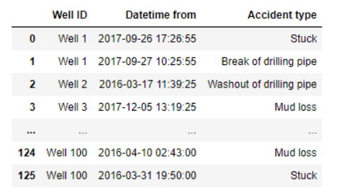
An expert analyzed each of the telemetry logs for the presence of anomaly behavior and why the particular accident occurred. For all cases, the expert uses only the telemetry parameters, presented in Table 2, and highlights the corresponding interval if abnormal behavior can be clearly distinguished in telemetry log data. An example of the expert reference table for all wells is given in Figure 2.
3.2 General scheme of the model
Based on methods considered in Section 2, the problem of drilling accident forecasting can be solved as a supervised machine learning problem trained on time-series database representation via the Bag-of-features approach. Let us consider two main steps of the model: feature generation and classification problem.
3.2.1 Feature generation
According to the Bag-of-features approach, we should assign one label from the codebook to the time series segment. To obtain the codebook of possible labels, we decided to train the clustering algorithm to assign the cluster number to the small segments of the time series, named segments. We also decided to represent the segment in the frequency domain using the wavelet transform since it is better represents the shape of the time series and better preserves similarity during shifting and stretching deformations. Since we mostly deal with non-stationary signals, Discrete Wavelet transform was chosen as the most promising one for such representation (Milon 2017; Sifuzzaman et al. 2009). The detailed description of the Discrete Wavelet transform might be found in paper (Tzanetakis et al. 2001), while the particular type of wavelet and level of decomposition used for the current problem will be discussed in section 4.
The scheme of the codebook construction process is shown in Figure 3 presented as pseudo-code in algorithm 1. The represented procedure was carried out separately for each of the drilling parameters in the following way:
- 1.
For each log presented in the database: split it into small parts of length , using sliding window technique with step ;
- 2.
Represent , using coefficients from Wavelet transform;
- 3.
Concatenate coefficients of wavelet transforms for each into the feature-matrix of -parts;
- 4.
Cluster the set of feature-vectors, obtained on the previous step, into clusters, using the k-means algorithm
- 5.
Use the trained clustering algorithm as a codebook.
Before the k-means procedure, we did not scale the set of feature-vectors since the scales of input features do not differ a lot (no more than ten times). Additionally, several variations of k-means algorithms were tried: usual k-means, k-means with different weights, k-means with assigning several clusters for one input sample. However, they did not bring significant differences in clustering quality metrics.

By obtaining the labels for all drilling parameters for segments, one could build a histogram of labels, predicted for the time series intervals, named segments, using the following steps:
- 1.
For each of the telemetry parameters, using sliding window technique with step , obtain the set of segments of length for the initial time series ;
- 2.
Divide each segment into small parts ;
- 3.
Assigning the label for each of the with trained KMeans algorithm, obtain the set of clusters labels for the particular ;
- 4.
Obtain the vector of features for the particular telemetry parameter and segment , building a histogram of labels distributions ;
- 5.
Combine the vectors for each telemetry parameter into one vector of features related to the segment .
The scheme of the feature generation procedure is shown in Figure 4 and presented as pseudo-code in algorithm 2. An example of the generated histogram for the particular part of telemetry log data is presented Appendix A. Using described strategy, one could obtain time-series database representation via the Bag-of-features approach and build the matrix of features for further experiments’ training and validation phases.

3.2.2 Classification problem
Since the model should forecast the probability of several types of drilling accidents, we use the multitarget strategy, where a single classifier is trained per class with the samples of that class as positive ones and all other samples as negatives. We decided to use a model based on the Gradient Boosting of decision trees for a single classifier. They are relatively undemanding in terms of sample size and data quality and learn quickly with a large number of features, which was also shown in papers (Burnaev et al. 2015; Kozlovskaia and Zaytsev 2017). In our case, we use Gradient Boosting algorithm with 50 estimators, learning rate equals 0.05, max depth of 10, while the subsample and colsample by tree correspond to 90%. In addition, we increased the weight of the positive class five times. Since we have an imbalanced dataset, we also tried under-sampling and oversampling techniques, however, none significantly improved model quality.
The training process uses mud telemetry intervals of hours long before the accident. As input values, the model uses features of selected intervals obtained during the feature generation phase (Section 3.2.1). During the model’s training, we assume that considered interval leads to drilling accidents if it was six hours before the beginning of the accident. Since the model’s purpose is to forecast the accident of all six possible types, we would not separate on different cases (e.g., mud losses can develop over time while pipe breaking may be a sudden event). Besides, if considered interval leads to several types of drilling accidents, a positive target value is assigned for all selected types. Since pre-accidents patterns differ by length, such six-hour intervals may contain parts of normal drilling behavior, marked as pre-accident ones. However, we will assume that their influence during model training will not be significant since the training sample will contain many similar normal intervals sampled from the rest of the training set, diluting the influence of normal intervals annotated as pre-accident.
During the real-time model performance, at each time moment, the model generates features for the last received part of data of length and returns the probability of whether the input data contains the pre-accident patterns for each of the accident’s types. Described procedure presented as pseudo-code in algorithm 3. The model can be switched on with different time steps, however, the model results will correspond only to when the model was switched on.
3.3 Validation procedures
To validate model performance, we build the Receiver operating characteristic (ROC) curve and calculate the area under it (ROC AUC metric). Since we deal with a multiclass classification problem, the current metric was calculated for each instance and then averaged. For the accident forecasting metrics, we assume that the accident was forecasted if the model alarm happened before the hours of the accident and the type was predicted correctly. Otherwise, the model warning was counted as a false alarm.
Metrics were calculated using a -fold cross-validation technique (Mohri et al. 2012). Scheme of cross-validation procedure is presented in Figure 5. Generating two random sets of non-intersecting wells, one could obtain train and test samples, picking the wells from the corresponding set. On each step, the train set always contains examples of all six accident types. The probability that all anomaly intervals of the same accident type will not appear in the training sample for some fold is less than 0.01 percent. The model was trained on the wells, which indices were chosen as train one. Validation carried out on the test set, which for each well includes the hour intervals before the accident and intervals of eight hours length of normal drilling behavior. Repeating the described procedure times, one could obtain the final ROC AUC score.
4 Results and discussions
4.1 Selection of the main hyperparameters
Before introducing the general model quality metrics, we conduct several experiments to select the primary model hyperparameters. The main hyperparameters’ scheme versus model steps is shown in Figure 6. We do not show the KMeans algorithm’s parameters on the scheme since tuning these parameters is carried out with common procedures, e.g., described in (Claesen and De Moor 2015; Bergstra et al. 2013). According to Figure 6, the drilling forecasting model has two main groups of parameters (blue and orange boxes), where parameters marked with one color mean that their selection took place within the same experiment.
Based on the experiment setup, one could notice that the true optimal combination may be different since all hyperparameters influence each other, and not all combinations were tested. However, since we have limited resources to run the full parameter optimization process, we use coordinate-wise optimization, which is one of the possible solutions for such problems (Friedman et al. 2007).
First, we conduct experimenters related to selecting parameters marked with blue color: wavelet type, level of decomposition, and the number of clusters. To compare different parameter sets, we obtain a reference matrix , which shows whether two intervals are similar () or not () in terms of drilling behavior. Matrix was obtained for the sample of segments intervals. For the particular set of model parameters, one could train the KMeans model with clusters, which as input uses the histogram of labels for interval, obtained with Bag-of-features approach, and as output gives the label of a cluster for the particular interval. Transforming the vector of predicted labels into a matrix , where each element indicates whether the interval and are in the same cluster, one could calculate the Rand Index, showing the similarity between the reference and obtained matrices:
| (1) | |||
| (2) | |||
| (3) | |||
| (4) | |||
| (5) |
Rand Index varies from zero to one, where means that reference and obtained matrices are identical. Comparing different sets of parameters using such metrics, one could find an optimal parameter setting for the current experiment. In Appendix B, one may see the top tested sets of parameters with the value of the metric obtained for the optimal . The best sets of parameters include the wavelet and KMeans algorithm with clusters. To assess the validity of the obtained results, we also calculated the baseline model’s metric value, where time-series values were directly used as a feature vector. Rand Index for the baseline approach was , which is lower than the best-obtained result, which was .
The results can additionally be validated visually. It can be done using the tsne technique that, as input, use a pairwise distance matrix between features of segments . Picking randomly several intervals and using their reference matrix values, we could obtain the groups of points corresponding to similar time series segments. The conducted test results for three randomly chosen time series intervals for the best set of parameters and baseline cases are shown in Figure 7. Bag-of-features representation gives us a better cluster distribution of similar time series segments than the baseline case.
We also tested the Bag-of-features model’s sensitivity to the number of clusters in both clustering algorithms for the best set of parameters. In Figure 8, one may see the Rand Index curves with a confidence interval for different and values, where is represented in the log scale. The obtained results show that the developed model is sensitive to small values of (from to ) and (from to ), while for other values, the Rand Index metric is almost the same. Since the best set of parameters was obtained for and included , the model with the obtained parameters setting can be used in further experiments.
The second stage of the parameter selection procedure includes selecting the length of segments and with fixed sets of parameters selected in the first experiment. The selection of these two parameters was carried out based on ROC AUC values obtained during cross-validation. In Table 4 one may see the ROC AUC scores for different sets of the lengths of segments and . If the segment was longer than the length of the segment, we assumed that the ROC AUC value is undefined. With the segments of length minutes and segments of length minutes model can forecast % of drilling accidents.
| t length, minutes | ||||
| 72 min | 180 min | 420 min | ||
| 8 min | 0.69 | 0.7 | 0.68 | |
| length, minutes | 24 min | 0.7 | 0.68 | 0.67 |
| 50 min | 0.68 | 0.69 | 0.68 | |
4.2 General model quality
As was mentioned in Section 3.3, the general model quality was estimated using the ROC curve and ROC AUC metric. To benchmark model quality with other models, we trained Convolution Neural Network (CNN), similar to the approaches (Aljubran et al. 2021; Qodirov and Shestakov 2020), which uses segment values as features, and random classifier, which predicts accident probabilities for each time step in segment randomly. CNN model has tree convolution units, where each convolution layer is followed by the batch normalization layer, dropout unit (p=0.1), and two fully connected linear layers with and input neurons, respectively. For the training, we use SGD optimizer and cross-entropy as loss functions. In addition, to compare the current model with previous studies, we retrained and validated the Breakdown model, presented in paper (Antipova et al. 2019), on the same samples used during the Bag-of-features quality estimation procedures. The breakdown model uses aggregated features, such as mean, slope, etc., over the interval and predicts the accident with the Gradient Boosting algorithm.
We tuned models’ hyperparameters for all models to increase the corresponding metrics values and achieve a fair comparison of the models. For the Bag-of-features and gradient boosting, we adjusted the number of trees, learning rate, and the fraction of observations to be selected for each tree. In contrast, we chose several convolutions layers, learning rate, the maximum number of epochs, and the dropout rate for the CNN model.
According to the model quality graph shown in Figure 9, the ROC AUC score for the Bag-of-features model is , while for the CNN, Random models, the ROC AUC score is and , respectively. Comparing the Bag-of-features model with the Breakdown model, the current model gives us a higher metric value.
Additionally, we validate model quality without considering multiclass classification, but only considering if there is an accident or not at a particular time moment. On Figure 10 one may see the corresponding ROC AUC values. Similar to the previous case, the Bag-of-features model performs better than other models.
Comparing the Bag-of-features performance for multiclass and binary problems, one may notice that the difference between ROC AUC metric values is insignificant. It means that the model clearly distinguishes the pre-accident situation of a different type, and most of the errors relate to the misinterpretation of whether the segment contains a pre-accident pattern or not.
According to Figure 9, the Bag-of-features model can forecast 70% of drilling accidents with a false positive rate equals to %. It corresponds to the four false alarms per day for one hour long. The high value of the false-positive rate for the model can be explained by the fact that the testing sample also contains anomaly behavior that did not lead to the accident, however, the model triggered that. An example of such a situation is shown in Figure 11. The yellow area stands for the anomaly behavior associated with an anomaly pressure drop that did not lead to the actual washout accident. In contrast, in the green zone, which corresponds to the six hours interval before another washout accident, one may observe similar pressure reduction, which leads to the washout accident in this case. The model alarmed the right types during both anomaly behavior intervals. However, according to the metric calculation scheme, the first two alarms were count as false ones. An additional expert evaluation of the mud logs, where such intervals will be highlighted as abnormal regions, is required to take into account such cases.

The current metric point corresponds to 70% of forecasted drilling accidents with a false positive rate equal to %, achieved with a false negative rate (FNR) equal to 30%. In Table 5 one could see the number of non-predicted cases for each accident type. The model is struggled with breaks and washouts of drilling pipe cases, while other accidents showed good results. It could be explained that the break of drilling pipe usually does not have any anomaly behavior before the accident. However, a detailed evaluation of such cases is necessary.
| Accident type | Number of non-predicted cases | Total number of cases | |
|---|---|---|---|
| 1 | Stuck | 5 | 55 |
| 2 | Washouts of drilling pipe | 8 | 20 |
| 3 | Mud loss | 5 | 16 |
| 4 | Breaks of drilling pipe | 12 | 15 |
| 5 | Fluid shows | 4 | 10 |
| 6 | Packing | 3 | 9 |
4.3 Optimisation of the model performance
The last experiment selected the frequency with which the model should be turned on during real-time testing. Fixing the parameters selected during previous stages, we obtained the metric values for different steps for segments generation (Figure 12). One may notice that using steps for segments generation less than one hour long does not significantly affect the model’s quality. Since there is still a probability of missing the non-standard behavior with more than minutes, we decided to use step equals minutes for further production testing.
4.4 Discussion and future work
Forecasting accidents during well drilling is essential for the oil and gas industry since it would help save time and money related to the accident consequences. Nowadays, it becomes evident that a combination of drilling engineers’ knowledge and machine learning models allows us to predict accidents of several selected types.
In a separate section, we conduct an ablation study of the model’s main hyperparameters. Conducted tests suggest that the current model is not sensitive to the changes in parameter setting. The Bag-of-features model was also compared to the other state-of-the-art models such as the CNN model, the Breakdown model, described in paper (Antipova et al. 2019), and the Random model. The developed model’s quality metrics exceed the quality of other models and ensure good performance during real-time drilling operations.
However, there is still room for improvement. In particular, it is interesting to conduct experiments to identify the dependence of model quality on the size of the accident database and obtain model quality, using other metrics that might indicate the ratio of true forecasted events and the particular number of false alarms per day. Besides, as mentioned in section 4.2, additional expert evaluation of the mud logs is required to take into account anomaly drilling behavior that happened outside the six-hour interval before the accident. It also might be a good strategy for the objective function during model training to assign higher penalties for false negatives of more severe drilling accidents.
Another problematic aspect of this method is the highly unbalanced classification problem since most data patterns are rare. Moreover, the patterns are fuzzy and can be distorted both in time and in the time series’ values by noise and scale. Thus, it is necessary to test and find another time series representation where such patterns might be better observed.
Nowadays model is testing in real oilfields in Russia. To operate the model, we developed software integrated with the Wellsite Information Transfer Standard Markup Language (WITSML) data server into clients’ existing IT infrastructure. All calculations take place on the cloud and, therefore, do not require significant additional computing power.
5 Conclusions
We have demonstrated that the model is generalizable from field to field. The scalability illustrates that the model tackles the key challenge of drilling accident forecasting: the lack of properly defined pre-accident patterns for different drilling regimes at different fields.
The novelty of the research is the Bag-of-features representation of multivariate telemetry logs and the machine learning model itself. Talking numbers, the developed model can forecast 70% of the accidents with a false positive rate equal to %, which is higher than the metrics of the state-of-the-art studies and random baseline. Moreover, obtained results show that model clearly distinguishes the pre-accident situation of a different type, and most of the errors relate to the misinterpretation of whether the segment contains a pre-accident pattern or not.
The intelligent system for real-time drilling accident prediction allows preventing drilling accidents and reducing costs associated with failures. In the future, we plan to develop the model further for pushing down the false positive rate and increasing the timing of correct predictions. For these purposes, we will work thoroughly with the training set marking the abnormal cases which are not followed by accident and developing the physics-informed filters on top of the core model.
References
- Abanda et al. (2019) Abanda A, Mori U, Lozano JA (2019) A review on distance based time series classification. Data Mining and Knowledge Discovery 33(2):378–412
- Abu-Abed (2010) Abu-Abed F (2010) Application of neural network modeling tools for analysis of pre-emergency situations on drilling sites. Software Products and Systems (3):136–139
- Abu-Abed (2015) Abu-Abed F (2015) Automated system for detection of pre-emergency situations at oil and gas industry facilities. Logger (5 (251)):48–61
- Ali and Frimpong (2020) Ali D, Frimpong S (2020) Artificial intelligence, machine learning and process automation: existing knowledge frontier and way forward for mining sector. Artificial Intelligence Review 53(8):6025–6042
- Aljubran et al. (2021) Aljubran M, Ramasamy J, Bassam M, Magana-Mora A (2021) Deep learning and time-series analysis for the early detection of lost circulation incidents during drilling operations. IEEE Access
- Antipova et al. (2019) Antipova K, Klyuchnikov N, Zaytsev A, Gurina E, Romanenkova E, Koroteev D, et al. (2019) Data-driven model for the drilling accidents prediction. In: SPE Annual Technical Conference and Exhibition, Society of Petroleum Engineers
- Bangert (2021) Bangert P (2021) Machine Learning and Data Science in the Oil and Gas Industry: Best Practices, Tools, and Case Studies. Gulf Professional Publishing
- Begum and Keogh (2014) Begum N, Keogh E (2014) Rare time series motif discovery from unbounded streams. Proceedings of the VLDB Endowment 8(2):149–160
- Bergstra et al. (2013) Bergstra J, Yamins D, Cox D (2013) Making a science of model search: Hyperparameter optimization in hundreds of dimensions for vision architectures. In: International conference on machine learning, pp 115–123
- Bostrom and Bagnall (2017) Bostrom A, Bagnall A (2017) Binary shapelet transform for multiclass time series classification. In: Transactions on Large-Scale Data-and Knowledge-Centered Systems XXXII, Springer, pp 24–46
- Burnaev et al. (2015) Burnaev E, Erofeev P, Papanov A (2015) Influence of resampling on accuracy of imbalanced classification. In: Eighth International Conference on Machine Vision (ICMV 2015), International Society for Optics and Photonics, vol 9875, p 987521
- Chandola et al. (2009) Chandola V, Banerjee A, Kumar V (2009) Anomaly detection: A survey. ACM computing surveys (CSUR) 41(3):15
- Claesen and De Moor (2015) Claesen M, De Moor B (2015) Hyperparameter search in machine learning. arXiv preprint arXiv:150202127
- Fawaz et al. (2019) Fawaz HI, Forestier G, Weber J, Idoumghar L, Muller PA (2019) Deep learning for time series classification: a review. Data Mining and Knowledge Discovery 33(4):917–963
- Ferreira et al. (2015) Ferreira APL, Carvalho DJ, Rodrigues RM, Schnell DM, Thomson IJ, Baptista RC, Alves SB, et al. (2015) Automated decision support and expert collaboration avoid stuck pipe and improve drilling operations in offshore brazil subsalt well. In: Offshore Technology Conference, Offshore Technology Conference
- Friedman et al. (2007) Friedman J, Hastie T, Höfling H, Tibshirani R, et al. (2007) Pathwise coordinate optimization. Annals of applied statistics 1(2):302–332
- Fu (2011) Fu Tc (2011) A review on time series data mining. Engineering Applications of Artificial Intelligence 24(1):164–181
- Grabocka et al. (2014) Grabocka J, Schilling N, Wistuba M, Schmidt-Thieme L (2014) Learning time-series shapelets. In: Proceedings of the 20th ACM SIGKDD international conference on Knowledge discovery and data mining, pp 392–401
- Grace (2017) Grace RD (2017) Blowout and well control handbook. Gulf Professional Publishing
- Gurina et al. (2020) Gurina E, Klyuchnikov N, Zaytsev A, Romanenkova E, Antipova K, Simon I, Makarov V, Koroteev D (2020) Application of machine learning to accidents detection at directional drilling. Journal of Petroleum Science and Engineering 184:106519
- Hajizadeh (2019) Hajizadeh Y (2019) Machine learning in oil and gas; a swot analysis approach. Journal of Petroleum Science and Engineering 176:661–663
- Hanley and McNeil (1982) Hanley JA, McNeil BJ (1982) The meaning and use of the area under a receiver operating characteristic (roc) curve. Radiology 143(1):29–36
- Hatami et al. (2019) Hatami N, Gavet Y, Debayle J (2019) Bag of recurrence patterns representation for time-series classification. Pattern Analysis and Applications 22(3):877–887
- Karim et al. (2019) Karim F, Majumdar S, Darabi H, Harford S (2019) Multivariate lstm-fcns for time series classification. Neural Networks 116:237–245
- Kozlovskaia and Zaytsev (2017) Kozlovskaia N, Zaytsev A (2017) Deep ensembles for imbalanced classification. In: 2017 16th IEEE International Conference on Machine Learning and Applications (ICMLA), IEEE, pp 908–913
- Kumar (2021) Kumar N (2021) Recent issues with machine vision applications for deep network architectures. In: Cognitive Computing Systems, Apple Academic Press, pp 267–284
- Li et al. (2020) Li H, Liu J, Yang Z, Liu RW, Wu K, Wan Y (2020) Adaptively constrained dynamic time warping for time series classification and clustering. Information Sciences 534:97–116
- Malhotra et al. (2017) Malhotra P, TV V, Vig L, Agarwal P, Shroff G (2017) Timenet: Pre-trained deep recurrent neural network for time series classification. arXiv preprint arXiv:170608838
- Milon (2017) Milon MH (2017) Comparison on fourier and wavelet transformation for an ecg signal. Am J Eng Res(AJER) 6(8):1–7
- Mohri et al. (2012) Mohri M, Rostamizadeh A, Talwalkar A (2012) Foundations of Machine Learning. The MIT Press
- Qodirov and Shestakov (2020) Qodirov S, Shestakov A (2020) Development of artificial neural network for predicting drill pipe sticking in real-time well drilling process. In: 2020 Global Smart Industry Conference (GloSIC), IEEE, pp 139–144
- Rakthanmanon and Keogh (2013) Rakthanmanon T, Keogh E (2013) Fast shapelets: A scalable algorithm for discovering time series shapelets. In: proceedings of the 2013 SIAM International Conference on Data Mining, SIAM, pp 668–676
- Sadlier et al. (2013) Sadlier A, Says I, Hanson R (2013) Automated decision support to enhance while-drilling decision making: Where does it fit within drilling automation? In: SPE/IADC Drilling Conference, OnePetro
- Sagheer and Kotb (2019) Sagheer A, Kotb M (2019) Unsupervised pre-training of a deep lstm-based stacked autoencoder for multivariate time series forecasting problems. Scientific reports 9(1):1–16
- Samhitha et al. (2020) Samhitha BK, Priya MS, Sanjana C, Mana SC, Jose J (2020) Improving the accuracy in prediction of heart disease using machine learning algorithms. In: 2020 International Conference on Communication and Signal Processing (ICCSP), IEEE, pp 1326–1330
- Schlumberger (2020) Schlumberger (2020) Oilfield glossary. URL https://www.glossary.oilfield.slb.com/en
- Serra and Arcos (2014) Serra J, Arcos JL (2014) An empirical evaluation of similarity measures for time series classification. Knowledge-Based Systems 67:305–314
- Sifuzzaman et al. (2009) Sifuzzaman M, Islam M, Ali M (2009) Application of wavelet transform and its advantages compared to fourier transform. Journal of Physical Sciences
- Tzanetakis et al. (2001) Tzanetakis G, Essl G, Cook P (2001) Audio analysis using the discrete wavelet transform. In: Proc. conf. in acoustics and music theory applications, Citeseer, vol 66
- Wang et al. (2013) Wang J, Liu P, She MF, Nahavandi S, Kouzani A (2013) Bag-of-words representation for biomedical time series classification. Biomedical Signal Processing and Control 8(6):634–644
- Wang et al. (2016) Wang X, Lin J, Senin P, Oates T, Gandhi S, Boedihardjo AP, Chen C, Frankenstein S (2016) Rpm: Representative pattern mining for efficient time series classification. In: EDBT
- Wang et al. (2017) Wang Z, Yan W, Oates T (2017) Time series classification from scratch with deep neural networks: A strong baseline. In: 2017 International joint conference on neural networks (IJCNN), IEEE, pp 1578–1585
- Yoon et al. (2019) Yoon J, Jarrett D, van der Schaar M (2019) Time-series generative adversarial networks. Advances in Neural Information Processing Systems 32 (NeurIPS 2019)
- Zheng et al. (2014) Zheng Y, Liu Q, Chen E, Ge Y, Zhao JL (2014) Time series classification using multi-channels deep convolutional neural networks. In: International Conference on Web-Age Information Management, Springer, pp 298–310
Appendix A
In Figure 13 one may see the example of mud telemetry data used during the drilling accident forecasting problem. After the feature generation procedure, the presented part of the time-series is transformed into a histogram, presented in Figure 14.
Appendix B
Table 6 shows the results of the first stage of an optimization procedure for the top parameter sets.
| K | level | Wavelet | Rand Index | N | |
| 1 | 200 | 3 | bior2.4 | 0.878484 | 25 |
| 2 | 100 | 5 | bior2.4 | 0.877657 | 25 |
| 3 | 100 | 4 | bior2.4 | 0.877504 | 25 |
| 4 | 100 | 4 | bior2.4 | 0.877341 | 25 |
| 5 | 100 | 4 | coif5 | 0.877247 | 25 |
| 6 | 200 | 4 | db3 | 0.877114 | 25 |
| 7 | 100 | 3 | coif5 | 0.876965 | 25 |
| 8 | 100 | 5 | coif5 | 0.87681 | 25 |
| 9 | 100 | 5 | db3 | 0.876686 | 25 |
| 10 | 100 | 4 | coif5 | 0.876612 | 25 |
| 11 | 200 | 3 | coif5 | 0.876277 | 25 |
| 12 | 100 | 3 | coif5 | 0.8762 | 25 |
| 13 | 100 | 3 | bior2.4 | 0.875928 | 22 |
| 14 | 100 | 5 | coif5 | 0.875765 | 22 |
| 15 | 200 | 3 | db3 | 0.875573 | 25 |
| 16 | 100 | 4 | bior2.4 | 0.875506 | 25 |
| 17 | 100 | 5 | bior2.4 | 0.875365 | 25 |
| 18 | 200 | 3 | bior2.4 | 0.875281 | 25 |
| 19 | 100 | 3 | bior2.4 | 0.875178 | 25 |
| 20 | 100 | 4 | coif5 | 0.875136 | 22 |
| 21 | 100 | 3 | coif5 | 0.875064 | 25 |
| 22 | 100 | 4 | db3 | 0.874835 | 25 |
| 23 | 100 | 5 | bior2.4 | 0.874827 | 22 |
| 24 | 200 | 4 | bior2.4 | 0.87479 | 25 |
| 25 | 200 | 3 | coif5 | 0.87478 | 25 |
| 26 | 100 | 3 | bior2.4 | 0.874499 | 25 |
| 27 | 100 | 5 | db3 | 0.874368 | 25 |
| 28 | 200 | 5 | coif5 | 0.874316 | 25 |
| 29 | 100 | 5 | coif5 | 0.874158 | 25 |
| 30 | 200 | 3 | db3 | 0.874094 | 25 |
| 31 | 200 | 3 | coif5 | 0.874079 | 25 |
| 32 | 200 | 4 | db3 | 0.874035 | 25 |
| 33 | 100 | 4 | db3 | 0.87396 | 25 |
| 34 | 100 | 4 | db3 | 0.87396 | 25 |
| 35 | 200 | 5 | bior2.4 | 0.873684 | 25 |
| 36 | 200 | 5 | bior2.4 | 0.87363 | 25 |
| 37 | 100 | 3 | db3 | 0.873504 | 25 |
| 38 | 200 | 3 | bior2.4 | 0.873353 | 25 |
| 39 | 200 | 5 | coif5 | 0.873131 | 25 |
| Baseline | Baseline | Baseline | Baseline | 0.840027 | 45 |