Training and Projecting: A Reduced Basis
Method Emulator for Many-Body Physics
Abstract
We present the reduced basis method as a tool for developing emulators for equations with tunable parameters within the context of the nuclear many-body problem. The method uses a basis expansion informed by a set of solutions for a few values of the model parameters and then projects the equations over a well-chosen low-dimensional subspace. We connect some of the results in the eigenvector continuation literature to the formalism of reduced basis methods and show how these methods can be applied to a broad set of problems. As we illustrate, the possible success of the formalism on such problems can be diagnosed beforehand by a principal component analysis. We apply the reduced basis method to the one-dimensional Gross-Pitaevskii equation with a harmonic trapping potential and to nuclear density functional theory for 48Ca, achieving speed-ups of more than x150 in both cases when compared to traditional solvers. The outstanding performance of the approach, together with its straightforward implementation, show promise for its application to the emulation of computationally demanding calculations, including uncertainty quantification.
Most modern theoretical models describing many-body nuclear dynamics share an ever-increasing computational burden. This can turn into a challenge tasks like uncertainty quantification (UQ) analysis Phillips et al. 2021; Ekström et al. 2019, experimental design Melendez et al. 2021a; Giuliani and Piekarewicz 2021, calibration of model parameters Pratt et al. 2015; McDonnell et al. 2015; Wesolowski et al. 2019, and even repeated evaluation for different inputs Lasseri et al. 2020; Godbey et al. 2022. Emulators—algorithms able to give fast-and-accurate approximate calculations to expensive computations—have been gaining increasing importance as a way to circumvent these challenges Santner et al. 2003; Phillips et al. 2021.
In recent years, a technique called eigenvector continuation (EC) Frame et al. 2018 was developed to emulate computationally intensive calculations involving bound states of Hamiltonian operators König et al. 2020 and nuclear scattering Furnstahl et al. 2020; Melendez et al. 2021b; Drischler et al. 2021. EC has shown excellent performance in interpolation and extrapolation by working with two elements: choosing its ansatz functions from the linear span of exact solutions to the problem at hand, and using a variational principle—for example the Rayleigh-Ritz method Frame et al. 2018; Cohen-Tannoudji et al. 1986a or the Kohn variational principle Furnstahl et al. 2020; Kohn 1948—to obtain equations for the coefficients of this linear combination.
We present an emulator constructed in the formalism of reduced basis methods (RBMs) Almroth et al. 1978; Quarteroni et al. 2015; Hesthaven et al. 2016, a set of dimensionality-reduction techniques that fall under the umbrella of reduced order models Quarteroni et al. 2014; Brunton and Kutz 2019; Melendez et al. 2022. These methods have seen active development over the last two decades, proving to be useful in a variety of computationally-intensive problems involving partial differential equations Quarteroni et al. 2011; Nguyen et al. 2010; Field et al. 2011; Milani et al. 2008. EC can be naturally connected to RBMs by constructing a generalization of EC through a Galerkin method formulation. The key insight is that once a reasonable choice of ansatz functions has been made (for example, the EC basis), all that is needed is a method to select a suitable candidate approximation from the ansatz subspace. This could be achieved, for instance, by using a variational principle, minimizing a cost functional, or by finding the fixed point of an iterative scheme. Among the alternatives, the Galerkin method—the option chosen in RBMs—stands out for its simplicity: it attempts to find an accurate approximate solution by projecting the problem to a well-chosen very-low dimensional subspace. This simplicity allows these methods to be applied to a wide variety of problems in a straightforward way.
RBMs are tailored to problems that feature an equation that depends smoothly on a list of tunable control parameters Quarteroni et al. 2015. The goal is to build an approximate solution for a suitable range of these parameters. Let us assume the equation is written in the general form:
| (1) |
where is a vector (or function) from a Hilbert space , and maps onto itself. For example, in the case of bound systems with a Hamiltonian that depends on , can take the form of the eigenvalue equation , where is the eigenvalue. Another example would be the case of single-channel scattering where can be the radial part of the scattering equation Thompson and Nunes 2009 , where a system with reduced mass interacts through a potential with parameters , is the angular momentum quantum number, and is the asymptotic linear momentum. The RBM finds approximate solutions to these—and more general—problems by constructing a basis expansion with linearly independent ‘reduced basis’ functions :
| (2) |
where is an extra term that can be added to satisfy boundary conditions imposed on Eq. (1). The reduced basis functions are selected to create an affine space (the ansatz subspace) close to the manifold formed by the solutions to Eq. (1) as a function of the parameters Quarteroni et al. 2015 by using the information from a (possibly small) sample of exact solutions. In practice, the ‘exact solutions’ (or ‘snapshots’) of Eq. (1) are constructed by highly accurate yet computationally expensive approximations such as finite element or spectral calculations Quarteroni et al. 2011.
An option for building the reduced basis in Eq. (2) is the approach taken in many EC applications Frame et al. 2018; König et al. 2020; Furnstahl et al. 2020; Melendez et al. 2021b; Drischler et al. 2021, also known as the Lagrange basis Quarteroni et al. 2011. It consists of calculating ‘training functions’ as solutions to Eq. (1) for values (), and then choosing the reduced basis as these training functions . One possible way to improve upon this choice is the so-called proper orthogonal decomposition (POD) Quarteroni et al. 2015. It consists of computing solutions and constructing the reduced basis with the first components from a principal component analysis (PCA) Jolliffe 2002, or singular value decomposition (SVD) Blum et al. 2020, of the set of these training functions. Therefore, by using the information of samples, the POD basis is more robust than a Lagrange basis of dimension , and faster than a Lagrange basis of training points. As a side note, an exponential decay on the associated singular values from the PCA indicates that the RBM can provide an accurate approximation for the problem at hand Quarteroni et al. 2011; Quarteroni et al. 2015; Nonino et al. 2019. We exploit this feature later when discussing Fig. 1.
Once the reduced basis functions are chosen, the coefficients for the approximation are found by the Galerkin method Rawitscher et al. 2018, that is, by projecting Eq. (1) over linearly independent ‘projecting functions’ in the Hilbert space:
| (3) |
is often called the residual Fletcher 1984, and it can be used, for example, to inform the construction of the reduced basis Buffa et al. 2012, or to estimate the emulation error Prud’homme et al. 2001. We can interpret Eq. (3) as enforcing the orthogonality of to the subspace spanned by , i.e., by finding a such that is “zero” up to the ability of the set . The choice of projecting functions is arbitrary, but is usually also informed by the solution manifold Quarteroni et al. 2015; Hesthaven et al. 2016. For the rest of this work, we choose to enforce orthogonality with respect to the ansatz subspace (2), which is the traditional way of using the Galerkin method Fletcher 1984.
The reduced-basis emulators are most effective, in terms of speed ups, when the projections in Eqs. (3) lead, for every , to expressions of the form:
| (4) |
where and are functions that are independent of the intrinsic coordinates of the original system. If these functions can be computed only once and then stored, we can avoid performing costly integrals or finite element calculations every time we have to solve Eqs. (3) for a new set of parameters . This property is exploited later when we construct an emulator for the Gross-Pitaevskii equation in Eq. (7).
To illustrate the application of the RBM and connect with previous results in the EC literature, we work with the two previously mentioned examples for . For the single-channel scattering example, we create the approximate solution , with as exact solutions to different , and satisfy the boundary conditions by imposing , as done in Furnstahl et al. 2020. By letting and thus , we explicitly satisfy the boundary condition while having only free coefficients. We identify for as the relevant elements in the basis expansion and select as the associated projecting functions, leading to the equations:
| (5) |
These equations—formulated from a geometric projection argument—are equivalent to those obtained by the Kohn variational principle Lucchese 1989, as done in Furnstahl et al. 2020; Drischler et al. 2021. The proof is elaborated in the supplementary material.
In the bound system example, with , Eq. (3) might not have a solution for the exact eigenvalue. Allowing to be approximated by helps ensure we can solve the projected equations:
| (6) |
where the set plus the approximate eigenvalue add up to unknowns. We can complete the set of equations with a normalization condition: . When choosing as exact solutions for different , Eq. (6) is equivalent to the generalized eigensystem of EC formulated from the Rayleigh-Ritz variational method Frame et al. 2018.
Beyond these two examples, the generality of the Galerkin formalism allows to apply RBMs to a wide variety of problems, including discrete, operator, integral, and differential equations Fletcher 1984; Singh and Stauffer 1974. As such, the projected equations (3) can be directly applied to non-linear problems like non-linear eigenvalue equations where , with a general operator. Additionally, in the case of coupled equations—common in many-body physics—the formalism is easily extended by expanding each coupled function independently and finding the coefficients by enforcing Eq. (3) with projecting functions for each -th coupled function.
It is important to note, however, that if the solution manifold for the problem at hand cannot be sufficiently embedded in a linear subspace, then the RBM we described will not constitute an effective emulator. We can engineer a simple example with the 1D quantum Hamiltonian of a particle trapped in an infinite well Cohen-Tannoudji et al. 1986b by letting control the location of the well. A direct application of the RBM fails to accurately emulate the ground state wavefunction as changes. Extensions to the basic methodology can tackle these issues by allowing further manipulation of the reduced basis Nonino et al. 2019.
In practice, to test whether a problem is fit for emulation via RBMs, it is sufficient to observe the decay of the singular values associated with the PCA of a group of exact solutions for various Quarteroni et al. 2015. Fig. 1 shows the singular values for the problems discussed in our work, all decaying exponentially except for the infinite well. In the case of the scattering wavefunctions in the channel at a fixed energy for the Minnesota potential Thompson et al. 1977, the are consistent with the EC results Furnstahl et al. 2020. A similar pattern is obtained for wavefunctions across energies (black squares in Fig. 1) by re-scaling the scattering differential equation via the change of variable , making all exact solutions share the same asymptotic behavior. This observation implies that in principle it should be possible to build a scattering emulator across energies. For the Gross-Pitaevskii equation and the 13 energy levels of 48Ca under density functional theory (DFT), the decay of their respective also makes them excellent candidates for the application of the RBM, as we explore next.

The Gross-Pitaevskii equation Gross 1961; Pitaevskii 1961 (see also Pichi et al. 2020 for a RBM application) is a nonlinear Schrödinger equation that approximately describes the low-energy properties of dilute Bose-Einstein condensates. Using a self-consistent mean field approximation, the many-body wavefunction is reduced to a description in terms of a single complex-valued wavefunction . We work with the one-dimensional Gross-Pitaevskii equation Carr et al. 2000a; Carr et al. 2000b; Carr et al. 2001; Torres-Vega 2017 with a harmonic trapping potential by letting be:
| (7) |
where , , and are proportional to the strength of the harmonic trapping, the self-coupling of the wavefunction, and the ground state energy, respectively. is a single variable function that depends on and it is normalized to unity. Note that, since this equation depends linearly on and , the projection Eqs. (3) that involve integrals in can be evaluated and stored for faster computation, leading to expressions of the form in Eq. (4). For example, the term associated with the harmonic trapping reads: .

To test the RBM for extrapolation, we built a Lagrange basis with four training functions in the space as exact solutions (), with the projecting functions as . Panel a) in Fig. 2 shows the results of emulating by using this basis and applying Eqs. (3) plus the normalization condition. The agreement between the exact and emulated calculations is excellent, with an error of less than in the repulsive phase () where the four training parameters are located, and it deteriorates only in the attractive phase () well beyond the training region. Extrapolation is not a feature usually exploited on the RBM literature, yet it could be key when calculations of exact solutions in a specific phase of the system are numerically unstable or impossible, but approximable by such methods.
In addition to extrapolating, we explored a situation similar to how emulators are tested for UQ König et al. 2020; Drischler et al. 2021. Using a Latin hypercube sampling (LHS) Mckay et al. 2000, we drew 500 testing points in the range and . We constructed three types of reduced basis: Lagrange, POD, and POD+Greedy, each with three sizes . The Lagrange basis consisted of exact solutions drawn with LHS. The POD and POD+Greedy consisted of principal components from a set of exact solutions. For the POD the exact solutions were drawn using LHS, while for the POD+Greedy the first solution was placed at a central location and the other were included one-by-one through a Greedy algorithm inspired on Refs. Veroy et al. 2003; Haasdonk and Ohlberger 2008; Sarkar and Lee 2021a. Our Greedy approach finds the parameter set for the next exact solution , by maximizing the norm of the residual over a LHS of parameters . In each step, is constructed with a POD basis informed by the previous exact solutions.
Table 1 shows the relative root mean squared errors (RMSEs), which converge exponentially as expected from the results in Fig. 1. Both POD bases were more accurate and robust than the Lagrange basis, which produced results that frequently changed by more than an order of magnitude when re-sampling the exact solutions for the basis. For the accuracy of the POD+Greedy basis was more than times better than the Lagrange basis. In terms of speed-up when calculating the 500 testing points, the three reduced bases with were almost times faster than the exact solver, while and obtained speed-ups of 40 and times, respectively.
| Basis n |
|
| ||||||
|---|---|---|---|---|---|---|---|---|
| Lagrange | POD |
|
POD | |||||
| 2 | ||||||||
| 4 | ||||||||
| 8 | ||||||||
We now proceed to use the RBM in realistic nuclear DFT calculations. DFT is a widely applied microscopic formalism Schunck 2019 (see also Cancès et al. 2007; Lin et al. 2012; Zhang et al. 2017 for other RBM applications to DFT). In nuclear physics it is used to describe properties of nuclei from the mean-field perspective, i.e., each nucleon interacts with an average effective field made up of all the particles in the system. This interaction is then constructed in a self-consistent way: the wavefunction of each nucleon and its eigenenergy are found at the same time as the effective field they produce and interact with. As such, the Hamiltonian acting on the -th wavefunction depends on all of them:
| (8) |
where , and the parameter list has been omitted for the sake of clarity. The dependence of the Hamiltonian on the wavefunctions comes from, for example, the total nuclear density and kinetic energy density . We derive the single particle Hamiltonian, , from the Skyrme effective interaction Skyrme 1956; Skyrme 1958; Vautherin and Brink 1972; Engel et al. 1975, the nuclear part of which can be written as a general energy density functional (EDF) of time-even densities Dobaczewski and Dudek 1995:
| (9) |
where the subscript represents isoscalar and isovector densities, respectively. The parameters of this EDF, for instance, model the coupling between the particles and the nucleonic density in question (the kinetic energy density, , in this case). As it is usually done in modern EDF optimization Chabanat et al. 1997; Kortelainen et al. 2010, we can parametrize those couplings in terms of nuclear-matter properties plus the remaining coupling constants left unconstrained:
| (10) |
This representation is primarily rooted in physical observables—like the nuclear saturation density, —and simplifies the selection of a sensible range of values to explore in model calibration for DFT, and for constructing the training bases for the RBM.
To test the RBM in extrapolation for DFT, we built a Lagrange basis of four points spanning MeV and MeV while the other parameters remained at their optimized UNEDF1 values Kortelainen et al. 2012. The wavefunctions on each shell (7 for neutrons and 6 for protons) were calculated using both the exact solver and the RBM emulator. Panel b) in Fig. 2 shows the performance of the emulator when calculating the neutron skin thickness of 48Ca Hagen et al. 2016, a quantity particularly sensitive to the parameter. The agreement between the emulated values and exact DFT results is excellent, with an error of less than for all extrapolated values shown, even for and well outside the training zone.
To test the limits of the emulator, the range of all ten available parameters in Eq. (10) were widened well beyond what is reasonable for realistic nuclear matter. We used LHS to draw 50 training points to build a POD basis with and to independently draw 500 testing points within the widened parameter ranges. As such, several parameter combinations yielded convergence issues for the DFT solver, but not for the emulated calculations, highlighting the capability of RBMs to extrapolate into regions where exact solvers can experience numerical instabilities. Even though the emulated results of non-converging test points seemed reasonable, we consider their validation to be beyond the scope of this work.
As Table 1 shows, for the stable parameter sets, the RBM reproduces single nucleon energies well. This is particularly striking for the reduced basis with only two elements, which gives an error of about despite all ten parameters being varied in the test sample. In terms of speed-up when calculating the 500 testing points, the reduced basis with were , , and times faster than the exact solver, respectively. We note that these speedups were obtained without precomputing any of the terms involved in Eq. (3). Greater speed-ups can be achieved by precomputing as many of the terms in Eq. (3) as possible, in the traditional strategy of an offline/online procedure often seen in RBM applications. Indeed, by separating the Hamiltonian in Eq. (8) into the parts that can and cannot be precalculated (called affine and non-affine in the RBM literature Quarteroni et al. 2015), we achieve speed-ups of more than 250 times with respect to the exact solver for a reduced basis of two elements.
The parts of the Hamiltonian (8) that are non-affine in the parameters can be made affine by using techniques such as the Empirical Interpolation Method Barrault et al. 2004; Grepl et al. 2007. The terms that are nonlinear in the wavefunctions on the other hand, such as powers of the density , can present a problem due to a combinatorially increasing terms () in Eq. (4). We will further study these challenges in a future work.
Speed-up gains of more than two orders of magnitude will enable large scale model UQ studies for a wide range of EDFs Giuliani et al. 2022, an endeavor which, up to now, seemed inaccessible. Furthermore, the RBM approach could also reduce the penalty of using higher-dimensional solvers for systematic studies and UQ, calculations previously limited to spherical and cylindrical symmetries. Finally, the trained emulators could be deployed in a cloud computing environment Godbey and Giuliani 2022, fostering collaborative research and facilitating the expansion of the scientific network.
We hope our results help spark the interest of the nuclear theory community in RBMs. For this purpose, we created and will continue to update an online resource Godbey et al. to illustrate many of the concepts we discussed. The adoption of recent developments on the choice of ansatz subspaces Benner et al. 2015; Ohlberger and Rave 2013; Nonino et al. 2019, on error bounds and convergence properties Veroy et al. 2003; Buffa et al. 2012; Cohen et al. 2020, and on the computational efficiency for non-affine and nonlinear problems Barrault et al. 2004; Grepl et al. 2007, to name a few, could become key in reaching the full extent of what these methods can offer. Given the simplicity and flexibility of the Galerkin projection, and the PCA diagnostic we showcase to test for low-dimensional manifolds, we believe that RBMs have the potential to become standard tools for the emulation of challenging problems in many-body nuclear physics.
Acknowledgements.
Acknowledgements
We are very grateful to Witek Nazarewicz and Frederi Viens for their critical observations during the elaboration of this manuscript. We also thank Ana Posada, Jorge Piekarewicz, and Daniel Phillips for their careful read of the manuscript. This work was supported by the National Science Foundation CSSI program under award number 2004601 (BAND collaboration), the U.S. Department of Energy under Award Number DOE-DE-NA0003885 (NNSA, the Stewardship Science Academic Alliances program), U.S. Department of Energy (DE-SC0013365 and DE-SC0021152) and the Nuclear Computational Low-Energy Initiative (NUCLEI) SciDAC-4 project (DE-SC0018083).
References
- Phillips et al. (2021) D. R. Phillips, R. J. Furnstahl, U. Heinz, T. Maiti, W. Nazarewicz, F. M. Nunes, M. Plumlee, M. T. Pratola, S. Pratt, F. G. Viens, and S. M. Wild, J. Phys. G Nucl. Part. Phys. 48, 072001 (2021).
- Ekström et al. (2019) A. Ekström, C. Forssén, C. Dimitrakakis, D. Dubhashi, H. T. Johansson, A. S. Muhammad, H. Salomonsson, and A. Schliep, J. Phys. G Nucl. Part. Phys. 46, 095101 (2019).
- Melendez et al. (2021a) J. Melendez, R. Furnstahl, H. Grießhammer, J. McGovern, D. Phillips, and M. Pratola, Eur. Phys. J. A 57, 1 (2021a).
- Giuliani and Piekarewicz (2021) P. G. Giuliani and J. Piekarewicz, Phys. Rev. C 104, 024301 (2021).
- Pratt et al. (2015) S. Pratt, E. Sangaline, P. Sorensen, and H. Wang, Phys. Rev. Lett. 114, 202301 (2015).
- McDonnell et al. (2015) J. D. McDonnell, N. Schunck, D. Higdon, J. Sarich, S. M. Wild, and W. Nazarewicz, Phys. Rev. Lett. 114, 122501 (2015).
- Wesolowski et al. (2019) S. Wesolowski, R. Furnstahl, J. Melendez, and D. Phillips, J. Phys. G Nucl. Part. Phys. 46, 045102 (2019).
- Lasseri et al. (2020) R.-D. Lasseri, D. Regnier, J.-P. Ebran, and A. Penon, Phys. Rev. Lett. 124, 162502 (2020).
- Godbey et al. (2022) K. Godbey, A. S. Umar, and C. Simenel, (2022), 10.48550/ARXIV.2206.04150.
- Santner et al. (2003) T. J. Santner, B. J. Williams, W. I. Notz, and B. J. Williams, The Design and Analysis of Computer Experiments, Vol. 1 (Springer, 2003).
- Frame et al. (2018) D. Frame, R. He, I. Ipsen, D. Lee, D. Lee, and E. Rrapaj, Phys. Rev. Lett. 121, 032501 (2018).
- König et al. (2020) S. König, A. Ekström, K. Hebeler, D. Lee, and A. Schwenk, Phys. Lett. B 810, 135814 (2020).
- Furnstahl et al. (2020) R. Furnstahl, A. Garcia, P. Millican, and X. Zhang, Phys. Lett. B 809, 135719 (2020).
- Melendez et al. (2021b) J. Melendez, C. Drischler, A. Garcia, R. Furnstahl, and X. Zhang, Phys. Lett. B 821, 136608 (2021b).
- Drischler et al. (2021) C. Drischler, M. Quinonez, P. Giuliani, A. Lovell, and F. Nunes, Phys. Lett. B 823, 136777 (2021).
- Cohen-Tannoudji et al. (1986a) C. Cohen-Tannoudji, B. Diu, and F. Laloe, Quantum Mechanics, Vol. 2 (John Wiley & Sons, 1986).
- Kohn (1948) W. Kohn, Phys. Rev. 74, 1763 (1948).
- Almroth et al. (1978) B. O. Almroth, P. Stern, and F. A. Brogan, AIAA J. 16, 525 (1978).
- Quarteroni et al. (2015) A. Quarteroni, A. Manzoni, and F. Negri, Reduced Basis Methods for Partial Differential Equations: An Introduction, Vol. 92 (Springer, 2015).
- Hesthaven et al. (2016) J. S. Hesthaven, G. Rozza, B. Stamm, et al., Certified Reduced Basis Methods for Parametrized Partial Differential Equations, Vol. 590 (Springer, 2016).
- Quarteroni et al. (2014) A. Quarteroni, G. Rozza, et al., Reduced order methods for modeling and computational reduction, Vol. 9 (Springer, 2014).
- Brunton and Kutz (2019) S. L. Brunton and J. N. Kutz, Data-driven science and engineering: Machine learning, dynamical systems, and control (Cambridge University Press, 2019).
- Melendez et al. (2022) J. A. Melendez, C. Drischler, R. Furnstahl, A. Garcia, and X. Zhang, Journal of Physics G: Nuclear and Particle Physics (2022), https://doi.org/10.1088/1361-6471/ac83dd.
- Quarteroni et al. (2011) A. Quarteroni, G. Rozza, and A. Manzoni, J. Math. Ind. 1, 1 (2011).
- Nguyen et al. (2010) N. C. Nguyen, G. Rozza, D. B. P. Huynh, and A. T. Patera, in Large‐Scale Inverse Problems and Quantification of Uncertainty (John Wiley & Sons, 2010) Chap. 8, pp. 151–177.
- Field et al. (2011) S. E. Field, C. R. Galley, F. Herrmann, J. S. Hesthaven, E. Ochsner, and M. Tiglio, Phys. Rev. Lett. 106, 221102 (2011).
- Milani et al. (2008) R. Milani, A. Quarteroni, and G. Rozza, Comput. Methods Appl. Mech. Eng. 197, 4812 (2008).
- Thompson and Nunes (2009) I. J. Thompson and F. M. Nunes, Nuclear Reactions for Astrophysics: Principles, Calculation and Applications of Low-Energy Reactions (Cambridge University Press, 2009).
- Jolliffe (2002) I. T. Jolliffe, Principal Component Analysis (Springer, 2002).
- Blum et al. (2020) A. Blum, J. Hopcroft, and R. Kannan, Foundations of Data Science (Cambridge University Press, 2020).
- Nonino et al. (2019) M. Nonino, F. Ballarin, G. Rozza, and Y. Maday, (2019), https://doi.org/10.48550/arXiv.1911.06598, arXiv:1911.06598 [math.NA] .
- Rawitscher et al. (2018) G. Rawitscher, V. dos Santos Filho, and T. C. Peixoto, in An Introductory Guide to Computational Methods for the Solution of Physics Problems (Springer, 2018) pp. 17–31.
- Fletcher (1984) C. A. Fletcher, Computational Galerkin Methods (Springer, 1984).
- Buffa et al. (2012) A. Buffa, Y. Maday, A. T. Patera, C. Prud’homme, and G. Turinici, ESAIM: Math. Model. Numer. Anal. 46, 595 (2012).
- Prud’homme et al. (2001) C. Prud’homme, D. V. Rovas, K. Veroy, L. Machiels, Y. Maday, A. T. Patera, and G. Turinici, J. Fluids Eng. 124, 70 (2001).
- Lucchese (1989) R. R. Lucchese, Phys. Rev. A 40, 6879 (1989).
- Singh and Stauffer (1974) S. Singh and A. Stauffer, Il Nuovo Cimento B (1971-1996) 22, 139 (1974).
- Cohen-Tannoudji et al. (1986b) C. Cohen-Tannoudji, B. Diu, and F. Laloe, Quantum Mechanics, Vol. 1 (John Wiley & Sons, 1986).
- Thompson et al. (1977) D. Thompson, M. LeMere, and Y. Tang, Nucl. Phys. A 286, 53 (1977).
- Gross (1961) E. P. Gross, Il Nuovo Cimento 20, 454 (1961).
- Pitaevskii (1961) L. P. Pitaevskii, JETP 13, 451 (1961).
- Pichi et al. (2020) F. Pichi, A. Quaini, and G. Rozza, SIAM J. Sci. Comput. 42, B1115 (2020).
- Carr et al. (2000a) L. D. Carr, C. W. Clark, and W. P. Reinhardt, Phys. Rev. A 62, 063610 (2000a).
- Carr et al. (2000b) L. D. Carr, C. W. Clark, and W. P. Reinhardt, Phys. Rev. A 62, 063611 (2000b).
- Carr et al. (2001) L. D. Carr, C. W. Clark, and W. P. Reinhardt, Int. J. Mod. Phys. B 15, 1663 (2001).
- Torres-Vega (2017) G. Torres-Vega, J. Phys. Conf. Ser. 792, 012054 (2017).
- Mckay et al. (2000) M. D. Mckay, R. J. Beckman, and W. J. Conover, Technometrics 42, 55 (2000).
- Veroy et al. (2003) K. Veroy, C. Prud’Homme, D. Rovas, and A. Patera, in 16th AIAA Comput. Fluid Dyn. Conf. (2003) p. 3847.
- Haasdonk and Ohlberger (2008) B. Haasdonk and M. Ohlberger, ESAIM: M2AN 42, 277 (2008).
- Sarkar and Lee (2021a) A. Sarkar and D. Lee, (2021a), 10.48550/arXiv.2107.13449, arXiv:2107.13449 [nucl-th] .
- Schunck (2019) N. Schunck, ed., Energy Density Functional Methods for Atomic Nuclei, 2053-2563 (IOP Publishing, 2019).
- Cancès et al. (2007) É. Cancès, C. L. Bris, Y. Maday, N. Nguyen, A. Patera, and G. Pau, in CRM Proceedings and Lecture Notes (American Mathematical Society, 2007) pp. 15–47.
- Lin et al. (2012) L. Lin, J. Lu, L. Ying, and E. Weinan, J. Comput. Phys. 231, 2140 (2012).
- Zhang et al. (2017) G. Zhang, L. Lin, W. Hu, C. Yang, and J. E. Pask, J. Comput. Phys. 335, 426 (2017).
- Skyrme (1956) T. H. R. Skyrme, Philos. Mag. 1, 1043 (1956).
- Skyrme (1958) T. Skyrme, Nucl. Phys. 9, 615 (1958).
- Vautherin and Brink (1972) D. Vautherin and D. M. Brink, Phys. Rev. C 5, 626 (1972).
- Engel et al. (1975) Y. Engel, D. Brink, K. Goeke, S. Krieger, and D. Vautherin, Nucl. Phys. A 249, 215 (1975).
- Dobaczewski and Dudek (1995) J. Dobaczewski and J. Dudek, Phys. Rev. C 52, 1827 (1995).
- Chabanat et al. (1997) E. Chabanat, P. Bonche, P. Haensel, J. Meyer, and R. Schaeffer, Nucl. Phys. A 627, 710 (1997).
- Kortelainen et al. (2010) M. Kortelainen, T. Lesinski, J. Moré, W. Nazarewicz, J. Sarich, N. Schunck, M. V. Stoitsov, and S. Wild, Phys. Rev. C 82, 024313 (2010).
- Kortelainen et al. (2012) M. Kortelainen, J. McDonnell, W. Nazarewicz, P.-G. Reinhard, J. Sarich, N. Schunck, M. V. Stoitsov, and S. M. Wild, Phys. Rev. C 85, 024304 (2012).
- Hagen et al. (2016) G. Hagen, A. Ekström, C. Forssén, G. Jansen, W. Nazarewicz, T. Papenbrock, K. Wendt, S. Bacca, N. Barnea, B. Carlsson, et al., Nat. Phys. 12, 186 (2016).
- Barrault et al. (2004) M. Barrault, Y. Maday, N. C. Nguyen, and A. T. Patera, C. R. Math. 339, 667 (2004).
- Grepl et al. (2007) M. A. Grepl, Y. Maday, N. C. Nguyen, and A. T. Patera, ESAIM: Math. Model. Numer. Anal. 41, 575 (2007).
- Giuliani et al. (2022) P. Giuliani, K. Godbey, E. Bonilla, F. Viens, and J. Piekarewicz, arXiv preprint arXiv: arXiv:2209.13039 (2022), https://doi.org/10.48550/arXiv.2209.13039.
- Godbey and Giuliani (2022) K. Godbey and P. Giuliani, “BMEX - The Bayesian Mass Explorer,” (2022).
- (68) K. Godbey, P. Giuliani, E. Bonilla, and E. Flynn, “Reduced-basis methods in nuclear physics,” https://kylegodbey.github.io/nuclear-rbm/.
- Benner et al. (2015) P. Benner, S. Gugercin, and K. Willcox, SIAM Review 57, 483 (2015).
- Ohlberger and Rave (2013) M. Ohlberger and S. Rave, C. R. Math. 351, 901 (2013).
- Cohen et al. (2020) A. Cohen, W. Dahmen, R. DeVore, and J. Nichols, ESAIM: M2AN 54, 1509 (2020).
- Ascher et al. (1995) U. M. Ascher, R. M. Mattheij, and R. D. Russell, Numerical solution of boundary value problems for ordinary differential equations (SIAM, 1995).
- (73) https://github.com/kylegodbey/nuclear-rbm/tree/paperarchive.
- Bedaque et al. (2021) P. Bedaque, A. Boehnlein, M. Cromaz, M. Diefenthaler, L. Elouadrhiri, T. Horn, M. Kuchera, D. Lawrence, D. Lee, S. Lidia, et al., Eur. Phys. J. A 57, 1 (2021).
- Sarkar and Lee (2021b) A. Sarkar and D. Lee, Phys. Rev. Lett. 126, 032501 (2021b).
- Golub and Van Loan (2013) G. H. Golub and C. F. Van Loan, Matrix computations (JHU press, 2013).
- Hotelling (1933) H. Hotelling, J. Educ. Psychol. 24, 417 (1933).
- Turk and Pentland (1991) M. Turk and A. Pentland, J. Cogn. Neurosci. 3, 71 (1991).
- Jolliffe and Cadima (2016) I. T. Jolliffe and J. Cadima, Phil. Trans. R. Soc. A 374, 20150202 (2016).
- Bender et al. (2003) M. Bender, P.-H. Heenen, and P.-G. Reinhard, Rev. Mod. Phys. 75, 121 (2003).
Appendix A Supplementary Material
Appendix B Equivalence of the Reduced basis method and Eigenvector Continuation under the Kohn Variational Principle
For the sake of conciseness, we only treat the case of eigenvector continuation applied to single-channel scattering, as done in Furnstahl et al. 2020 using the Kohn Variational principle. The extension to the generalized Kohn principle Drischler et al. 2021; Lucchese 1989 is straightforward and follows the same steps shown below.
Within this context, we aim at finding approximate solutions to a differential equation of the form Thompson and Nunes 2009:
| (S1) |
where represent the potential the particle interacts with, which we assume changes smoothly with its parameter set , is the angular momentum quantum number and relates to the asymptotic momentum. Let us assume that the solution to this equation is subject to the boundary conditions , and
| (S2) |
Note that Eq. (S2) imposes a normalization condition on : the coefficient accompanying the sine function must equal .
A straightforward application of the reduced basis method (RBM) as discussed in the main document leads to the choice of an approximate function:
| (S3) |
where the are solutions to with the correct boundary conditions. Following the discussion on the main text, we eliminate the redundancy of the coefficients created by the boundary conditions by explicitly writing one of the them in terms of the others. Without loss of generality, we let , obtaining:
| (S4) |
With this rewriting, it becomes explicit that we only need to determine coefficients to obtain the approximate solution, which is part of the affine space spanned by . Following a similar reasoning to the main text, we choose for , resulting in the following equations for the remaining :
| (S5) | ||||
for where the inner product is defined as (without the usual complex conjugation).
We can rewrite Eq. (S5) in a more compact form by reintroducing , and the normalization condition. This results in the equation set:
| (S6) | |||
| (S7) |
B.1 Approximation through the Kohn Variational Principle
The (-matrix) Kohn variational principle (KVP) states that the solution to Eq. (S1) with the asymptotic behavior (S2), is a stationary point for the functional:
| (S8) |
where extracts its value from the asymptotic behavior of , that is, the cosine coefficient in Eq. (S2).
The Kohn variational method is detailed in the supplemental material of Ref. Furnstahl et al. 2020. It utilizes a trial function constructed exactly as in Eq. (S3), and it finds a stationary point of the functional (S8) in terms of the coefficients . After using the method of Lagrange multipliers to enforce the normalization condition, it is found that the following equation set describes the stationary point:
| (S9) |
where is the cosine coefficient in Eq. (S2) associated with each , and the matrix is a shorthand notation for the inner products:
| (S10) |
These equations, together with the normalization condition , can be used to find the coefficients , plus the Lagrange multiplier .
B.2 Proof of equivalence between the methods
To compare Eq. (S9) to Eq. (S6), we need to rewrite Eq. (S9) in terms of only, eliminating both the and the Lagrange multiplier . We can relate the elements of to their transposes by integration by parts. Note that
| (S11) |
where the boundary term can be evaluated through the boundary conditions (S2) to be . Therefore, via integration by parts, we can make act on in Eq. (S10) to obtain:
| (S12) |
Using this result we can eliminate from Eq. (S9) and obtain:
| (S13) | ||||
for ; where we used the fact that the sum to unity to cancel the term.
Next, we can eliminate the Lagrange multiplier and the sum of by subtracting equations for different . Without loss of generality, we can subtract all equations to the equation corresponding to , resulting in:
| (S14) |
Finally, using the definition of shows the equivalence with Eq. (S6), completing the proof.
It is interesting to note that the second term in Eq. (S2) can be thought as a first-order correction to the emulated . This correction adds a factor proportional to the residual , in a similar spirit as Newton’s method Ascher et al. 1995. The ‘proportionally factor’ (or transfer function Giuliani and Piekarewicz 2021) connecting the residual and is in this case the negative of the exact solution . This in turn, can be approximated by the emulated solution , obtaining the correction:
| (S15) |
Such first order correction, together with the POD+Greedy algorithm we used in the main text, highlight the fact that the residual is information rich and can be useful to improve the performance of the RBM emulator.
Appendix C Reduced Basis Method on a set of coupled equations
As we described in the main text, the RBM can be applied to the case with a set of coupled equations:
| (S16) |
by approximating each as a linear combination of their corresponding solutions for different values of :
| (S17) | ||||
By selecting as the generators of the affine spaces for each , we obtain the Galerkin equations:
| (S18) |
for to obtain the coefficients .
In the case of coupled eigenvalue-eigenvector systems, we can proceed as in the case of a single equation, by substituting the eigenvalues for approximate values , and enforcing normalization conditions, in accordance with the requirements of the problem at hand.
Appendix D Details about the numerical results
The codes used to generate all the results we presented in the main text and here can be found in rbm.
D.1 Decay of singular values
In this section, we give details on the construction of the singular values from the singular value decomposition (SVD) showed in Fig. 1 of the main text. Four problems were considered: the infinite well (IW), the single channel 2-body scattering with a Minnesota potential at fixed energy (SM) and varying energy (SM), the Gross-Pitaevskii equation (GP), and 48Ca under density functional theory (DFT). Fig S1 shows, for all problems considered, solutions for 10 different values of their parameters (left column), and the first 4 principal components out of a sample of 40 parameters in each case (right column).
The IW problem consists of the 1D quantum Hamiltonian of a particle trapped in an infinite well (IW) Cohen-Tannoudji et al. 1986b where controls the location of the well:
| (S19) |
The ground state solutions to this Hamiltonian are wave functions of the form for and zero otherwise. The singular values for the IW showed in Fig. 1 of the main text were obtained by sampling 40 values of in the range using Latin hypercube sampling (LHS), and performing SVD on the set of 40 solutions. The do not decay exponentially, and as can be seen in Fig. S1 the first 4 principal components are unable to capture the variability of the set of solutions. As mentioned in the main text, extensions to the basic RBM Nonino et al. 2019, such as allowing the training functions to be re-scaled and shifted in their domain, are able to tackle these issues. In this particular example, taking advantage of the symmetry of the problem, i.e., , would lead to all to be zero for .
Both SM and SM problems consist of the single-channel nucleon-nucleon scattering Hamiltonian Thompson and Nunes 2009. The Minnesota potential Thompson et al. 1977 with parameters is used for the interaction:
| (S20) |
where the other two non-linear parameters were fixed. In both cases, we make the change of variables and the scattering Hamiltonian takes the form:
| (S21) |
where the potential is now momentum dependent: . In both cases, (SM and SM) 40 parameters where obtained by a LHS in the range MeV and MeV, following Furnstahl et al. 2020. The singular values showed in Fig. 1 of the main text were obtained by performing SVD on the set of 40 solutions. In the case of SM, all 40 solutions shared the same energy in the center of mass MeV, while for SM the energies where equispaced in the range MeV.
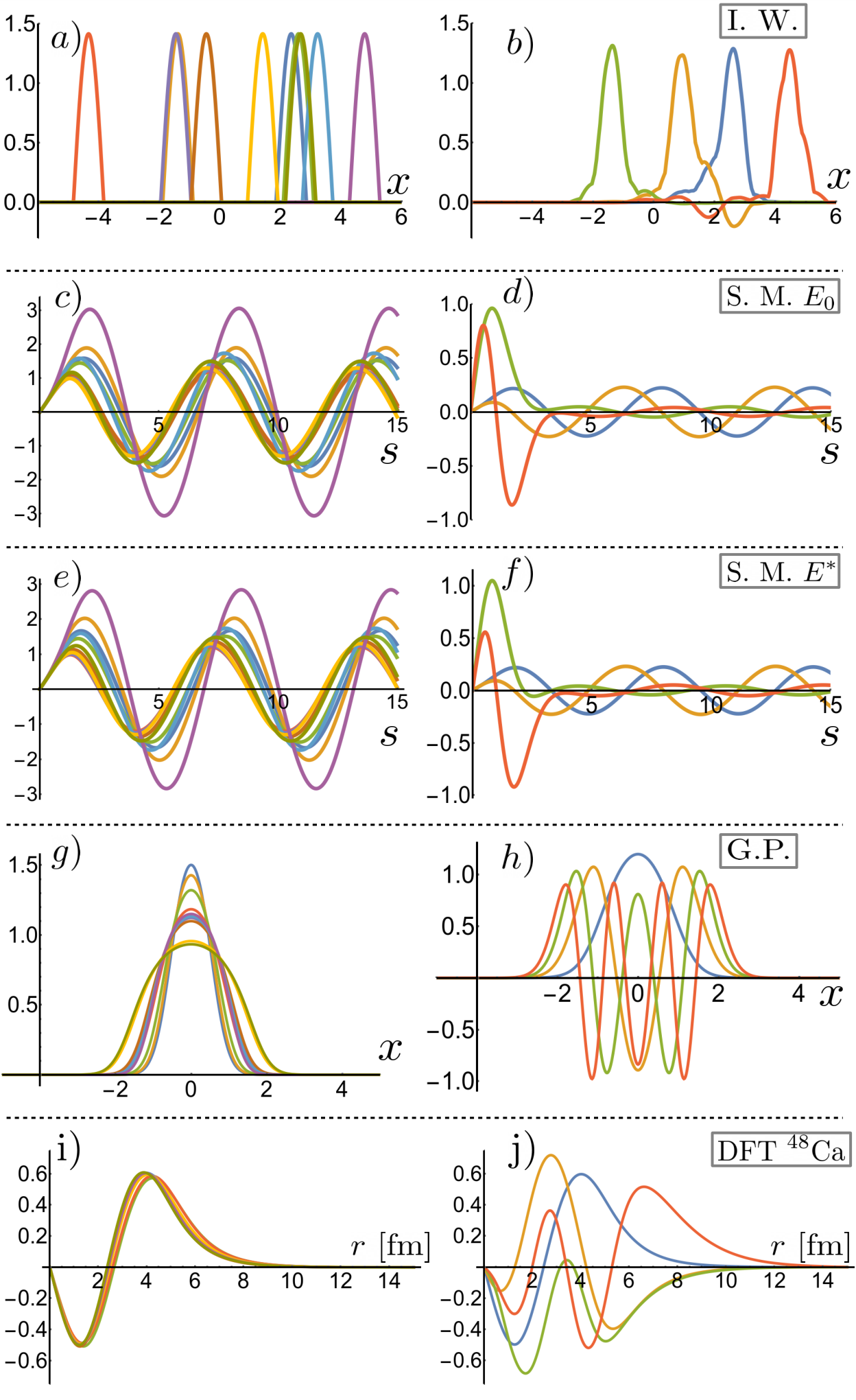
The GP and DFT cases are explained in detail in the main text. The ranges for the parameters in both cases correspond to the ones used in Table I of the main text. For GP, a set of 40 values of the parameters were obtained by LHS in the range and . For DFT, 50 values of the parameters were obtained with a LHS across the parameter ranges shown in Table S1.
D.2 1-D Gross-Pitaevskii equation with a harmonic trapping potential
The four training points used in the Lagrange basis for the results of Fig. 2 a) in the main text are : . Fig. S2 shows the training points for the Lagrange and POD RB, as well as the 500 testing points used for the results shown in Table I in the main text. Fig. S3 shows the construction on the POD+Greedy basis also used for the results shown in Table I in the main text. Fig. S4 shows the 20 exact solutions selected by the Greedy algorithm, as well as the first four principal components of this set.
Find s.t.
for do
Draw parameters with LHS:
Use the RBM with the RB to find for each element in
Find s.t.
end for
| Min | Max | Units | |
| 0.14 | 0.18 | fm-3 | |
| E/A | -16.5 | -14.5 | MeV |
| K | 160 | 260 | MeV |
| a | 26 | 32 | MeV |
| L | 20 | 180 | MeV |
| M | 0.7 | 1.4 | |
| -55 | -40 | MeV fm5 | |
| -165 | -90 | MeV fm5 | |
| -105 | -55 | MeV fm5 | |
| -50 | -15 | MeV fm5 |
D.2.1 Description of the POD+Greedy scheme used for GP
The POD+Greedy scheme used for the results of Table I of the main text consists on iteratively constructing a set of exact solutions () with a (weak) Greedy algorithm Quarteroni et al. 2015 informed by the residuals of a POD RB of dimension derived from the set of exact solutions at each step. To set up the algorithm, let be a function that returns a normalized basis constructed with first principal components of the set of solutions if , and returns if . This function can be used to construct a POD basis of size up to with a set of solutions. The Greedy strategy we used is summarized in Algorithm 1. The desired POD bases were constructed by running on the output of this algorithm with , , , and .
D.3 Spherical Nuclear Density Functional Theory
The four training points, , used in Fig. 2 b) of the main text only varied the and parameters, with the rest taken to be the standard UNEDF1 optimal parameters Kortelainen et al. 2012. The four values of and , in MeV, are:
Table S1 shows the parameter ranges used for the LHS for the DFT results in Table I of the main text. Both the 500 testing points and the exact evaluations used to build the POD RB were independently drawn by LHS on these ranges.
Appendix E Glossary of terminology


Table S2 shows the frequently used terms in this work (inspired by Bedaque et al. 2021).
| Acronym | Name | Brief Description | Detailed Ref. |
|---|---|---|---|
| EC | Eigenvector Continuation | Numerical method for approximating the “trajectory” of an eigenvector associated with a parametrized operator as the corresponding parameters change. As shown in this article, it can be seen as a special case of the RBM. | Frame et al. 2018; Sarkar and Lee 2021b |
| RBM | Reduced Basis Method | Numerical method for solving parametrized differential equations efficiently by using a handful of previously computed solutions. | Chapters 3 in Hesthaven et al. 2016; Quarteroni et al. 2015 |
| SVD | Singular Value Decomposition | Matrix factorization algorithm key for many modern computational methods, including PCA and POD. | Chapter 1 in Brunton and Kutz 2019, Chapter 2 in Golub and Van Loan 2013 |
| POD | Proper Orthogonal Decomposition | SVD application to partial differential equations used to capture a low-dimensional representation of the corresponding dynamical system. In the context of RBMs it is used to construct small bases that capture a low-dimensional representation of a larger set of “exact” solutions. | Sec. 3.3.1 in Hesthaven et al. 2016 , Chapter 6 in Quarteroni et al. 2015, Sec. 11.1 in Brunton and Kutz 2019 |
| PCA | Principal Component Analysis | SVD application where the variability of high-dimensional data is decomposed into its more statistically descriptive factors. | Chapter 1 in Brunton and Kutz 2019, Hotelling 1933; Turk and Pentland 1991; Jolliffe and Cadima 2016 |
| LHS | Latin Hypercube Sampling | Sampling technique for efficiently distributing points in . | Mckay et al. 2000 |
| - | Greedy Algorithm | Algorithm that selects the locally optimal choice on each iteration. In the context of RBMs, it sequentially selects “exact” solutions to train the emulator, usually by maximizing an estimated error. | Sec. 3.2.2 in Hesthaven et al. 2016, Chapter 7 in Quarteroni et al. 2015, Sarkar and Lee 2021a |
| - | Lagrange Basis | A reduced basis of size for the RBM that is built as a linear combination of only “exact” solutions. | Quarteroni et al. 2011 |
| DFT | Density Functional Theory | Mean-field approach to many-body quantum systems. | Bender et al. 2003; Schunck 2019 |
| EDF | Energy Density Functional | The object that defines the interaction used in DFT. | Bender et al. 2003; Schunck 2019 |
