Transferring Dual Stochastic Graph Convolutional Network for Facial Micro-expression Recognition

As shown in Figure 2, our proposed method consists of two parts. The upper part is the source network by macro-expression images and the bottom part is the target network by micro-expression images.

In source network, the input macro images are normalized in the pre-processing step. Macro images are fed into stochastic graph convolutional network. After each layer of stochastic graph convolution, an activation layer and pooling layer are appended. The classification is accomplished by computing the loss function at the fully connected layer. The SGCNs trained by source network are transferred to the target network.

In target network, there are two branches including spatial and temporal branch. The inputs of spatial and temporal branch are micro pixel images and optical flow images, respectively. In spatial branch, we use optical flow method to realize frame normalization to select meaningful frames in the entire micro-expression sequence. To improve the recognition performance, we adopt two transferred SGCNs (SGCN1 and SGCN2) to extract features, named dual SGCN (DSGCN). In temporal branch, we also utilize transferred SGCN1 and SGCN2 to extract features. Features from spatial and temporal branch are integrated to represent the discriminative features. The integrated features are fed into a fully connected layers.

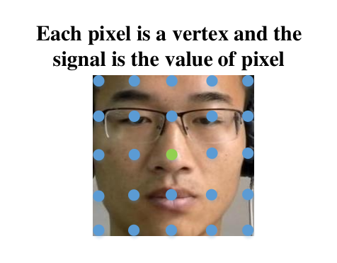
We first give the detail of how our stochastic graph construction works. Given an image $I$, we convert it into an undirected and connected graph $\mathcal{G}=(\mathcal{V},\mathcal{E},\mathbf{A})$. $\mathcal{V}$ is a finite set of $|\mathcal{V}|=N$ vertices, where each node is corresponding to a pixel. $\mathcal{E}$ is a finite set of edges, which are decided by their neighbors. $\boldsymbol{x}\in\mathbb{R}^{N}$ represents the signal defined on the graph where $x_{i}$ is the value of pixel at the $i^{th}$ node.

Our work presents a novel $p+q$ graph construction method. Each vertex has $p$ nearest neighbors and $q$ neighbors stochastically selected. The adjacency matrix $\mathbf{A}$ associated to $\mathcal{G}$ can be constructed. For node $i\in\{1\cdots N\}$, we design a distance threshold $T$ to select its potential neighbors. We calculate the Euclidean distance $d(z_{i},z_{j})$ between node $i$ and node $j$, where $z_{i}$ is node $i$’s 2D coordinate. If $d_{ij}$ is not more than threshold $T$, node $j$ is a neighbor of node $i$, $j\sim i$. Otherwise, there is no edge between node $i$ and $j$. The weighs between node $i$ and node $j$ are calculated in (1) and the number of node $i$’s neighbors is denoted by $|\mathcal{N}_{i}|$.

where $z_{i}$ is the 2D coordinate of pixel $i$ and the $\sigma$ is the average distance between each vertex and the vertex that is the farthest from it.

Algorithm 1 gives the details of our adjacent matrix construction. For node $i$, we extract its potential neighbors $\mathcal{N}_{i}$ by (1) with given threshold $T$. We choose $p$ nearest neighbors as fixed neighbors. We compute the weights of $p$ nearest neighbors by Gaussian kernel function. We stochastically choose $q$ neighbors among the left. The weights of remaining neighbors are zero.

Figure 3 gives an example of $p=8$ and $q=2$ graph construction for the reference node with green color. We design the distance threshold $T=2\sqrt{5}$. There are 24 potential neighbors for the middle reference node. We choose 8 nearest neighbors as fixed neighbors. We stochastically select 2 neighbors from the left blue vertices. The remaining ones are unlinked.

We propose a dual network to integrate two different SGCNs (SGCN1 and SGCN2). SGCN1 uses the $p_{1}+q_{1}$ graph construction and SGCN2 uses $p_{2}+q_{2}$ graph construction. We use transfer learning to achieve feature extraction in our dual network. We use macro images to train the SGCN in source network. We use the trained model to extract features from micro images in the target network.

As illustrated in Section III-B, we construct different adjacency matrices $\mathbf{A}_{1}$ and $\mathbf{A}_{2}$ corresponding to SGCN1 and SGCN2. The corresponding Laplacian matrices $\mathbf{L}_{1}$ and $\mathbf{L}_{2}$ are computed as

where $\mathbf{D}_{1}$ and $\mathbf{D}_{2}$ are the diagonal degree matrices with $\mathbf{D}_{1}(i,i)=\sum\nolimits_{j}\mathbf{A}_{1}(i,j)$ and $\mathbf{D}_{2}(i,i)=\sum\nolimits_{j}\mathbf{A}_{2}(i,j)$. $\mathbf{I}_{N}\in\mathbb{R}^{N\times N}$ is the identity matrix.

There are $L$ stochastic graph convolutional layers in our dual network. We utilize the truncated Chebyshev polynomials to achieve the graph convolutional filtering [11]. For layer $l$, the output feature is denoted as $\mathbf{X}^{l}\in\mathbb{R}^{M\times d_{l}}$, where $M$ is the number of input samples and $d^{l}$ is the dimension of output features. The convolutional coefficients $\boldsymbol{w}^{l}\in\mathbb{R}^{K^{l}}$ are trained by macro images in source network, where $K^{l}$ denotes the truncated order of Chebyshev polynomials in $l$-th layer. The dual stochastic graph convolution for the $l$-th layer ($1\leq l\leq L$) is implemented

where $\boldsymbol{w}^{1}_{k}$ and ${\color[rgb]{0,0,1}\boldsymbol{w}^{2}_{k}}$ are trained weights from the source network by macro images. $\tilde{\mathbf{L}}_{1}=\frac{2}{\lambda_{1_{max}}}\mathbf{L}_{1}-\mathbf{I}_{N}$ and $\lambda_{1_{max}}$ denotes the largest eigenvalues of $\mathbf{L}_{1}$. $\tilde{\mathbf{L}}_{2}=\frac{2}{\lambda_{2_{max}}}\mathbf{L}_{2}-\mathbf{I}_{N}$ and $\lambda_{2_{max}}$ denotes the largest eigenvalues of $\mathbf{L}_{2}$. The interval of the eigenvalues in $\tilde{\mathbf{L}}$ is $[-1,1]$.

We feed the outputs of $L$-th layer $\mathbf{X}^{L}_{1}\in\mathbb{R}^{M\times d_{L}}$ and $\mathbf{X}^{L}_{2}\in\mathbb{R}^{M\times d_{L}}$ into the trained fully connected layer. The outputs of fully connected layer are denoted as $\mathbf{X}^{fc}_{1}\in\mathbb{R}^{M\times d_{fc1}}$ and $\mathbf{X}^{fc}_{2}\in\mathbb{R}^{M\times d_{fc2}}$, where $d_{fc1}$ and $d_{fc2}$ are the dimensions of fully connected layer in SGCN1 and SGCN2, respectively.

After concatenation, the fused features of dual network are as follows

In our proposed model, the spatial branch is designed to capture the spatial relationships between pixels across different frames. As we have mentioned in Section I, optical flow images can provide temporal information between different frames. The spatial and temporal features of micro-expressions at different expression-states are encoded using DSGCNs.

The feature extraction in the spatial branch is shown in Figure 4. Specifically, given a video, the spatial branch of $m$-th frame is represented as $\mathcal{G}_{m}=(\mathcal{V}_{m},\mathcal{E}_{m},\mathbf{A}_{m})$, where $m=1\cdots M_{s}$ and $M_{s}$ is the number of image sequences selected from the video. As shown in Section III-B, there are $N_{s}$ nodes in each image and the signal defined on the image is $\boldsymbol{x}\in\mathbb{R}^{N}_{s}$. The initial input features are represented by $\mathbf{X}_{s}^{in}=(\mathbf{x}_{1},\mathbf{x}_{2},\cdots,\mathbf{x}_{M_{s}})\in\mathbb{R}^{M_{s}\times N_{s}}$, where $\mathbf{x}_{m}$ is the signal of $m$-th image. We feed the initial features $\mathbf{X}_{s}^{in}$ into the transferred DSGCN. By Eq. (2), (3) and (4), we obtain the output features of spatial branch $\boldsymbol{X}_{s}^{D}\in\mathbb{R}^{M_{s}\times(d_{fc1}+d_{fc2})}$.

The feature extraction in temporal branch is shown in Figure 5. We compute the optical flow features between sequences. We select $M_{t}$ samples from the optical flow sequences. The initial input features of temporal branch are represented by $\mathbf{X}_{t}^{in}\in\mathbb{R}^{M_{t}\times N_{t}}$, where $M_{t}$ is the number of pixels of optical flow image. We also feed the initial features $\mathbf{X}_{t}^{in}$ into the transferred DSGCN. By Eq. (2), (3) and (4), we obtain the output features of temporal branch $\boldsymbol{X}_{t}^{D}\in\mathbb{R}^{M_{t}\times(d_{fc1}+d_{fc2})}$.

We concatenate the features $\boldsymbol{X}_{s}^{D}$ and $\boldsymbol{X}_{t}^{D}$ obtained by spatial and temporal branches,

We train a fully connected layer by the fused features $\boldsymbol{X}^{in}$ in target network. The output feature of the target network is denoted by $\boldsymbol{X}^{out}\in\mathbb{R}^{(M_{s}+M_{t})\times d_{fc3}}$, where $d_{fc3}$ is the dimension of fully connected layer appended by the spatial and temporal branch.

Lin et al. [30] proposed the definition of focal loss to handle the class imbalance in scene detection. The focal loss is defined as:

where $\alpha$ is a weighting factor to balance the importance for positive and negative example, $\gamma$ is the focusing parameters to balance the difference between easy and hard examples. $y\in\{0,1\}$ is the ground-truth label and $p\in[0,1]$ is the model’s estimated probability for the class with label $y=1$.

To evaluate our proposed approach, we conduct experiments using two databases: SAMM (the most commonly used) and MMEW (a newly published).

MMEW As a newly published dataset, there are $300$ samples in micro-and-macro expression warehouse (MMEW) [3], including happiness (36), anger (8), surprise (89), disgust (72), fear (16), sadness (13) and others (102), which is the biggest published micro-expression dataset. There are 36 participants including 9 females and 27 males, whose average age is 22.35. 900 macro-expression samples with the same category by the same group of participants are also provided.

SAMM The Spontaneous Actions and Micro-Movements (SAMM) contains 159 samples (image sequences containing spontaneous micro-expressions) recorded by a high-speed camera in a well controlled laboratory environment [9, 10, 51]. There are 32 participants with a mean age of 33.24 years, and an even male-female gender split. Originally intended for investigating micro-facial movements, the SAMM was induced based on the 7 basic emotions including happiness (24), surprise (13), anger (20), disgust (8), sadness (3), fear (7), others (84).

As shown in [3], the performance results of published algorithms on micro-expression recognition are reported across different experimental settings. Ben et al. conduct a fair comparison on datasets SAMM and MMEW, which are the most suitable datasets for recognition evaluation. We design the same experimental settings as [3]. In the MMEW dataset, 226 samples from 5 classes (i.e., happiness, surprise, disgust, fear, sadness) were used; in the SAMM dataset, 72 samples from 5 classes (i.e., happiness, surprise, anger, disgust, fear) were used.

The network configuration of SGCN is designed in Table I. There are six stochastic convolutional layers. $K^{l}$ is the order of the ChebNet filter in the $l$-th layer , $d^{l}$ denotes the feature number of undirected graphs output from the $l$-th layer to the next layer, $s_{l}$ represents the number of times of graph coarsening in the $l$-th layer, $d_{fc}$ represents the size of fully connected layer.

The networks are trained using adaptive epochs or early stopping with a maximum set to 100 epochs. Basically, the training for each fold will stop when the loss score stops improving. We use Adaptive Moment Estimation (ADAM) as the optimizer, with a learning rate of $10^{-5}$ and decay of $10^{-6}$.

To validate the effectiveness of our proposed method on the micro-expression recognition problem, we compare our proposed method with several recent state-of-the-art methods on MMEW and SAMM. All the published results in [3] are also kept for the convenience of comparison. Table II summarizes the comparison results.

It is obvious that all deep learning methods perform better than those utilizing handcrafted features. It can be seen that our proposed method achieves the best recognition performance ( 72.7% on MMEW and 75.0% on SAMM), which outperforms state-of-the-art method TLCNN ( the best recognition performance is 69.4% on MMEW and 73.5% on SAMM) [42].

The success of TLCNN [42] demonstrates that the knowledge of macro-expressions is useful for micro-expression recognition under the CNN architecture. This paper explores the transferring macro-expression knowledge to assist micro-expression recognition based on the GCN architecture. The training and testing sets of MMEW and SAMM were set as [3]. Table III lists the data source and accuracy of the pre-training, fine-tuning and testing results for each experiment. Compared to existing methods, our proposed method considers the stochastic geometric features of different pixels, which can provide more discriminative and robust information. These experimental results validate the superiority of our method.

Results on MMEW We design efficient parameters of focal loss on MMEW. The results are presented in Table IV. The best result is $72.73\%$ occurs with the parameters $\alpha=1.5$ and $\gamma=0.2$. We also present confusion matrices in Figure 6, from which we observe that in MMEW, the “disgust” and “surprise” samples can be highly recognized on MMEW, instead the “fear” samples are difficult to train. Because the number of fear samples of MMEW is only 16, which is too small to train a good classifier.

Results on SAMM We also design efficient parameters of focal loss on SAMM. The results of different weight factor $\alpha$ and focus factor $\gamma$ are presented in Table V. The best result $75.00\%$ occurs with the parameters $\alpha=1$and $\gamma=1$. The confusion matrix in Figure 7 indicates that our method can totally recognize ”Happiness”, ”Surprise” and ”Angry”. It is difficult to train ”Disgust” and ”Fear” since their small samples.

For further analysis, we perform an extensive ablation study by removing certain portions of our proposed TSDGCN to see how that affects performance. This was carried out using the databases MMEW and SAMM.

To verify the impact of DGCN, we train both single and dual GCN for the spatial branch and temporal branch under the same setting as Table III. We select 10 sets of typical graph architectures containing 4 single GCN and 6 DGCN. For the convenience, we utilize the cross entropy loss here. The extensive experimental results on both MMEW and SAMM are reported in Table VI. It is obvious that most DGCNs obtain higher accuracies of pre-training, fine-tuning and testing than single GCNs. Comparing the testing accuracies, the best graph architecture is 8+2 and 4+0 on both MMEW and SAMM, which is marked in bold. We also observe that all the spatial branches have better recognition performance than temporal ones.

To verify the impact of spatial branch and the temporal branch, we train the “Spatial branch” and “Temporal branch” under the same experiment setting and graph architecture. With the aid of Table VI, we discuss the graph architecture 8+2 and 4+0. The experimental results on both MMEW and SAMM are reported in Table VII. On MMEW, the recognition accuracy of “Spatial + CE” is 65.9% and the recognition accuracy of “Temporal + CE” is only 45.7%. The performance of “Spatial + Temporal branch + CE” varies with 8+2 and 4+0 graph architecture is the better than “Spatial + CE” and “Temporal branch + CE”, which shows that “Temporal branch” compensates the performance of “Spatial branch”. On SAMM, the recognition accuracy of “Spatial + CE” is 68.8% and the recognition accuracy of “Temporal + CE” is only 36.9%. The performance of “Spatial + Temporal branch + CE” is the same with “Spatial+ CE”, which means “Temporal branch” doesn’t improve the performance. Fig. 8 shows mean and variance of optical flow sequences on MMEW and SAMM. It is obvious that optical flow sequences of MMEW vary among samples and optical flow sequences of SAMM change a few. It means temporal branch may not contain useful information, which is why temporal branch doesn’t improve the performance in SAMM.

To verify the impact of focal loss, we compare the recognition performance between cross entropy and focal loss under the same architecture settings. “Spatial+Temporal branch + FL” achieves the best performance on both MMEW and SAMM with the graph architecture 8+2 and 4+0, which shows the advantage of focal loss function.

Our proposed method may not have significant improved results when the dataset doesn’t contain efficient temporal information.

References

- [1] James Atwood and Don Towsley. Diffusion-convolutional neural network. Adv. Neural Inform. Process. Syst., pages 2001–2009, 2016.
- [2] Xianye Ben, Xitong Jia, Rui Yan, Xin Zhang, and Weixiao Meng. Learning effective binary descriptors for micro-expression recognition transferred by macro-information. Pattern Recognition Letters, 107:50–58, 2018.
- [3] Xianye Ben, Yi Ren, Junping Zhang, Su jing Wang, Kidiyo Kpalma, Weixiao Meng, and Yong-Jin Liu. Video-based facial micro-expression analysis: A survey of datasets, features and algorithms. IEEE Trans. Pattern Anal. Mach. Intell., Early access, 2021.
- [4] Braj Bhushan. Study of facial micro-expressions in psychology. Understanding facial expressions in communication, pages 265–286, 2015.
- [5] Joan Bruna, Wojciech Zaremba, Arthur Szlam, and Yann LeCun. Spectral networks and locally connected networks on graphs. Int. Conf. Learn. Represent., 2014.
- [6] Xinlei Chen, Li-Jia Li, Fei-Fei Li, and Abhinav Gupta. Iterative visual reasoning beyond convolutions. IEEE Conf. Comput. Vis. Pattern Recog., pages 7239–7248, 2018.
- [7] Ciprian A. Corneanu, Marc Oliu, Jeffrey F. Cohn, and Sergio Escalera. Survey on RGB, 3D, thermal, and multimodal approaches for facial expression recognition: History, trends, and affect-related applications. IEEE Trans. Pattern Anal. Mach. Intell., 38(8):1548–1568, 2016.
- [8] Adrian K. Davision, Moi Hoon Yap, and Cliff Lansley. Micro-facial movement detection using individualised baselines and histogram based descriptors. IEEE International Conference on Systems, Man, and Cybernetics, pages 1864–1869, 2015.
- [9] Adrian K. Davison, Cliff Lansley, Nicholas Costen, Kevin Tan, and Moi Hoon Yap. Samm: A spontaneous micro-facial movement dataset. IEEE Transactions on Affective Computing, 9(1):116–129, 2016.
- [10] Adrian K. Davison, Walied Merghani, and Moi Hoon Yap. Objective classes for micro-facial expression recognition. IEEE Transactions on Affective Computing, 4(10):119, 2018.
- [11] Michaël Defferrard, Xavier Bresson, and Pierre Vandergheynst. Convolutional neural networks on graphs with fast localized spectral filtering. Adv. Neural Inform. Process. Syst., pages 3844–3852, 2016.
- [12] Paul Ekman. Emotions revealed: Recognizing faces and feelings to improve communication and emotional life. Holt Paperback, 128(8):140–140, 2003.
- [13] Paul Ekman. Lie catching and microexpressions. The philosophy of deception, pages 118–133, 2009.
- [14] Y. Gan, Sze-Teng Liong, Wei-Chuen Yau, Yen-Chang Huang, and Lit-Ken Tan. Off-apexnet on micro-expression recognition system. Signal Processing: Image Communication, 74:129–139, 2019.
- [15] Justin Gilmer, Samuel S. Schoenholz, Patrick F. Riley, Oriol Vinyals, and George E. Dahl. Neural message passing for quantum chemistry. Int. Conf. on Machine Learning, pages 1263–1272, 2017.
- [16] Jiachi He, Jian-Fang Hu, Xi Lu, and Wei-Shi Zheng. Multi-task mid-level feature learning for micro-expression recognition. Pattern Recognition, 66:44–52, 2017.
- [17] Kaiming He, Xiangyu Zhang, Shaoqing Ren, and Jian Sun. Deep residual learning for image recognition. IEEE Conf. Comput. Vis. Pattern Recog., pages 770–778, 2016.
- [18] Berthold K.P. Horn and Brian G. Schunck. Determining optical flow. Artificial Intelligence, 17(1):185–203, 1981.
- [19] Chunlong Hu, Dengbiao Jiang, Haitao Zou, Xin Zuo, and Yucheng Shu. Multi-task micro-expression recognition combining deep and handcrafted features. IEEE International Conference on Pattern Recognition, pages 946–951, 2018.
- [20] Xiaohua Huang, Sujing Wang, Xin Lin, Guoying Zhao, Xiaoyi Feng, and Matti Piteikainen. Discriminative spatio temporal local binary pattern with revisited integral projection for spontaneous facial micro-expression recognition. IEEE Transactions on Affective Computing, 10:32–47, 2017.
- [21] Xiaohua Huang, Sujing Wang, Guoying Zhao, and Matti Piteikainen. Facial microexpression recognition using spatiotemporal local binary pattern with integral projection. Int. Conf. Comput. Vis., pages 1–9, 2015.
- [22] Sijie Ji, Kai Wang, Xiaojiang Peng, Jianfei Yang, Zhaoyang Zeng, and Yu Qiao. Multiple transfer learning and multi-label balanced training strategies for facial AU detection in the wild. IEEE Conf. Comput. Vis. Pattern Recog., pages 1657–1661, 2020.
- [23] Huaiqian Khor, John See, Raphael C.W.Phan, and Weiyao Lin. Enriched long-term recurrent convolutional network for facial micro-expression recognition. IEEE International Conference on Automatic Face and Gesture Recognition, pages 234–778, 2018.
- [24] Dae Hoe Kim, Wissam J. Baddar, and Yong Man Ro. Micro-expression recognition with expression-state constrained spatio-temporal feature representations. ACM Int. Conf. Multimedia, pages 382–386, 2016.
- [25] Thomas N. Kipf and Max Welling. Semi-supervised classification with graph convolutional networks. Int. Conf. Learn. Represent., 2017.
- [26] Loic Landrieu and Martin Simonovsky. Large-scale point cloud semantic segmentation with superpoint graphs. IEEE Conf. Comput. Vis. Pattern Recog., pages 4558–4567, 2018.
- [27] Shan Li and Weihong Deng. Reliable crowdsourcing and deep locality-preserving learning for facial expression in the wild. IEEE Conf. Comput. Vis. Pattern Recog., pages 2584–2593, 2017.
- [28] Shan Li and Weihong Deng. Reliable crowdsourcing and deep locality-preserving learning for unconstrained facial expression recognition. IEEE Trans. Image Process., 28(1):356–370, 2019.
- [29] Yante Li, Xiaohua Huang, and Guoying Zhao. Can micro-expression be recognized based on single apex frame . IEEE International Conference on Image Processing, pages 3094–3098, 2018.
- [30] Tsung-Yi Lin, Priya Goyal, Ross Grishick, Kaiming He, and Piotr Dollr. Focal loss for dense object detection. Int. Conf. Comput. Vis., pages 2980–2988, 2017.
- [31] Yong-Jin Liu, Bing-Jun Li, and Yu-Kun Lai. Sparse MDMO: Learning a discriminative feature for spontaneous micro-expression recognition. IEEE Transactions on Affective Computing, 12(1):254–261, 2018.
- [32] Yong-Jin Liu, Jin-Kai Zhang, Wen-Jing Yan, Su-Jing Wang, Guoying Zhao, and Xiaolan Fu. A main directional mean optical flow feature for spontaneous micro-expression recognition. IEEE Transactions on Affective Computing, 7(4):299–310, 2016.
- [33] Ling Lo, Hong-Xia Xie, Hong-Han Shuai, and Wen-Huang Cheng. MER-GCN: Micro-expression recognition based on relation modeling with graph convolutional networks. IEEE Conference on Multimedia Information Processing and Retrieval, pages 79–84, 2020.
- [34] Alessio Micheli. Neural network for graphs: a contextual constructive approach. IEEE Transactions on Neural Networks, 20(3):498–511, 2009.
- [35] Ali Mollahosseini, Behzad Hasani, and Mohammad H. Mahoor. Affectnet: A database for facial expression, valence, and arousal computing in the wild. IEEE Transactions on Affective Computing, 10:18–31, 2019.
- [36] Mathias Niepert, Don Mohamed Ahmed, and Konstantin Kutzkov. Learning convolutional neural networks for graphs. Int. Conf. on Machine Learning, pages 2014–2023, 2016.
- [37] Timo Ojala, Matti Pietikainen, and Topi Maenpaa. Multiresolution gray-scale and rotation invariant texture classification with local binary patterns. IEEE Trans. Pattern Anal. Mach. Intell., 24(7):971–987, 2002.
- [38] Davangini Patel, Xiaopeng Hong, and Guoying Zhao. Selective deep features for micro-expression recognition. IEEE International Conference on Pattern Recognition, pages 2258–2263, 2017.
- [39] Min Peng, Chongyang Wang, Tong Chen, Guangyuan Liu, and Xiaolan Fu. Dual temporal scale convolutional neural network for micro-expression recognition. Frontiers in Psychology, 8:1745–1756, 2017.
- [40] Min Peng, Zhan Wu, Zhizhao Zhang, and Tong Chen. From macro to micro expression recognition: deep learning on small datasets using transfer learning. IEEE International Conference on Automatic Face and Gesture Recognition, pages 657–661, 2018.
- [41] Avinash Ravichandran Riawan Chaudhry, Gregory Hager, and Rene Vidal. Histograms of oriented optical flow and binet-cauchy kernels on nonlinear dynamical systems for the recognition of human actions. IEEE Conf. Comput. Vis. Pattern Recog., pages 1932–1939, 2009.
- [42] Sujing Wang, Bingjun Li, Yongjin Liu, Wenjing Yan, Xinyu Ou, Xiaohua Huang, Feng Xu, and Xiaolan Fu. Micro-expression recognition with small sample size by transferring long-term convolutional neural network. Neurocomputing, 312:251–262, 2018.
- [43] Sujing Wang, Wen-Jing Yan, Xiaobai Li, Guoying Zhao, Chun-Guang Zhou, Xiaolan Fu, Minghao Yang, and Jianhua Tao. Micro-expression recognition using color spaces. IEEE Trans. Image Process., 24(12):6034–6047, 2015.
- [44] Sujing Wang, Wen-Jing Yan, Guoying Zhao, Xiaolan Fu, and Chunguang Zhou. Micro-expression recognition using robust principal component analysis and local spatiotemporal directional features. Eur. Conf. Comput. Vis., pages 325–338, 2014.
- [45] Yangan Wang, John See, Raphael C.-W. Phan, and Yee-Hui Oh. Efficient spatio-temporal local binary patterns for spontaneous facial micro-expression recognition. PLoS ONE, 10(5):e0124674, 2015.
- [46] Yangan Wang, John See, Raphael C.-W. Phan, and Yee-Hui Oh. LBP with six intersection points: Reducing redundant information in LBP-TOP for micro-expression recognition. Asian Conf. on Comput. Vis., pages 382–386, 2016.
- [47] Zonghan Wu, Shirui Pan, Fengwen Chen, Guodong Long, Chengqi Zhang, and Philip S Yu. A comprehensive survey on graph neural networks. IEEE Transactions on Neural Networks and Learning Systems, 32(1):4–24, January 2021.
- [48] Zhaoqiang Xia, Wei Peng, Huaiqian Khor, Xiaoyi Feng, and Guoying Zhao. Revealing the invisible with model and data shrinking for composite-database micro-expression recognition. IEEE Trans. Image Process., 29:8590–8605, 2020.
- [49] Hong-Xia Xie, Ling Lo, Hong-Han Shuai, and Wen-Huang Cheng. AU-assisted graph attention convolutional network for micro-expression recognition. ACM Int. Conf. Multimedia, pages 79–84, 2020.
- [50] Feng Xu, Junping Zhang, and James Z. Wang. Micro-expression identification and categorization using a facial dynamics map. IEEE Transactions on Affective Computing, 8(2):254–267, 2017.
- [51] Chuin Hong Yap, Connah Kendrick, and Moi Hoon Yap. Samm long videos: a spontaneous facial micro- and macro-expressions dataset. IEEE International Conference on Automatic Face and Gesture Recognition, pages 771–776, 2020.
- [52] C. Zach, T. Pock, and H. Bischof. A duality based approach for realtime TV-L1 optical flow. Pattern Recognition, pages 214–223, 2007.
- [53] Guoying Zhao and Matti Paetikainen. Dynamic texture recognition using local binary patterns with an application to facial expressions. IEEE Trans. Pattern Anal. Mach. Intell., 29(6):915–928, 2007.
- [54] Yuan Zong, Xiaohua Huang, Wenming Zheng, Zhen Cui, and Guoying Zhao. Learning from hierarchical spatiotemporal descriptors for microexpression recognition. IEEE Trans. Multimedia, 20(11):3160–3172, 2018.
- [55] Yuan Zong, Wenming Zheng, Xiaohua Huang, Jingang Shi, Zhen Cui, and Guoying Zhao. Domain regeneration for cross-database micro-expression recognition. IEEE Trans. Image Process., 27(5):2484–2498, 2018.
- [56] Yuan Zong, Wenming Zheng, ZhenCui, Guoying Zhao, and Bin Hu. Toward bridging micro-expressions from different domain. IEEE Transactions on Cybernetics, 50(12):5047–5060, 2019.