Adaptive Trajectory Prediction via Transferable GNN
Abstract
Pedestrian trajectory prediction is an essential component in a wide range of AI applications such as autonomous driving and robotics. Existing methods usually assume the training and testing motions follow the same pattern while ignoring the potential distribution differences (e.g., shopping mall and street). This issue results in inevitable performance decrease. To address this issue, we propose a novel Transferable Graph Neural Network (T-GNN) framework, which jointly conducts trajectory prediction as well as domain alignment in a unified framework. Specifically, a domain-invariant GNN is proposed to explore the structural motion knowledge where the domain-specific knowledge is reduced. Moreover, an attention-based adaptive knowledge learning module is further proposed to explore fine-grained individual-level feature representations for knowledge transfer. By this way, disparities across different trajectory domains will be better alleviated. More challenging while practical trajectory prediction experiments are designed, and the experimental results verify the superior performance of our proposed model. To the best of our knowledge, our work is the pioneer which fills the gap in benchmarks and techniques for practical pedestrian trajectory prediction across different domains.
1 Introduction
Trajectory prediction aims to predict the future trajectory seconds to even a minute prior from a given trajectory history. It plays an indispensable role in a large number of real world applications such as autonomous driving, robotics, navigation, video surveillance, and so on. In self-driving scenario, accurate pedestrian trajectory prediction is essential for planning Bai2015Intention; ma2020optimal, decision making Yuanfu2018PORCA, environmental perception Talbot2020Robot; Obo2020Intelligent, person identification Luber2010People, and anomaly detection Musleh2010Identifying; 2004Pedestrian. Trajectory prediction is a challenging task. For instance, strangers tend to walk alone trying to avoid collisions but friends tend to walk as a group Moussaid2010TheWalking. In addition, pedestrians can interact with surrounding objects or other pedestrians, while such interaction is too complex and subtle to quantify. To consider such interactions, a pooling layer is designed in work Social-LSTM alahi2016social to pass the interaction information among pedestrians, and then a long short-term memory (LSTM) network is applied to predict future trajectories. Following this pattern, many methods liang2019peeking; zhang2019sr; hu2020collaborative; xu2020cf; zhu2021simultaneous have been proposed for sharing information via different mechanisms, i.e., attention mechanism or similarity measure. Instead of predicting one determined future trajectory, some generative adversarial network-based (GAN) fernando2018gd; gupta2018social; li2019conditional; sadeghian2019sophie; dendorfer2021mg and encoder-decoder-based methods Mangalam2020It; cheng2020exploring; salzmann2020trajectronplusplus; xu2021tra2tra; chen2021personalized; chen2021human; shafiee2021introvert have been proposed to generate multiple feasible trajectories.

| Metric | Trajectory Domains | E-D | S-D | ||||
| ETH | HOTEL | UNIV | ZARA1 | ZARA2 | |||
| NoS | 70 | 301 | 947 | 602 | 921 | 877 | 383.63 |
| NoP | 181 | 1053 | 24334 | 2253 | 5833 | 24153 | 10073.07 |
| AN | 2.586 | 3.498 | 25.696 | 3.743 | 6.333 | 23.11 | 9.78 |
| AV () | 0.437 | 0.178 | 0.205 | 0.369 | 0.206 | 0.259 | 0.11 |
| AA () | 0.131 | 0.06 | 0.035 | 0.039 | 0.026 | 0.105 | 0.04 |
However, these existing methods usually focus on learning a generic motion pattern while ignoring the potential distribution differences between the training and testing samples. We argue that this learning strategy has some limitations. Fig. 1 illustrates one basic concept. It is obvious that the trajectories of walking pedestrians in different trajectory domains are different, the trajectory in the left figure is stable but the trajectory in the right figure is much more tortuous. The original strategy is to learn these two samples together without considering distribution differences, which introduces domain-bias and disparities into the model.
In order to quantitatively and objectively evaluate the potential domain gaps, Table 1 gives five numerical statistics of five commonly used trajectory domains. We can observe that the number of pedestrians in UNIV is much larger than that in ETH, and the differences among five trajectory domains are significant. As for pedestrian moving pattern, pedestrians in ETH have the largest average moving velocity, which is nearly three times larger than that in HOTEL. In addition, pedestrians in ETH also have the largest average moving acceleration, which is nearly five times larger than that in ZARA2. The E-D value and S-D value also reveal the huge differences among five different trajectory domains. This situation is general and always exists in practical applications. For example, in vision applications, cameras located in different cities/corners could lead to significant distribution gap. Similar situations are also common in robot navigation or autonomous driving-related applications since the environments are constantly changing.
To further demonstrate this challenge, we apply three state-of-the-art methods, Social-STGCNN mohamed2020social, SGCN shi2021sgcn, Tra2Tra xu2021tra2tra to demonstrate the performance drop when it comes to different trajectory domains. We take ETH as the example, these models are trained on the validation set of ETH and evaluated on the standard testing set of ETH. Note that there is no overlap trajectory sample between the training and testing set, but the distributions of them can be regarded as consistent. We refer to this evaluation setting as “consistent setting” and the performance under this new protocol as “updated ADE” and “updated FDE”. Fig. 2 shows the updated ADE/FDE as well as the original ADE/FDE reported in their papers. The performance drops are significant which further reveal the domain-bias problem in the original leave-one-out setting.
Domain adaptation (DA) is a subcategory of transfer learning which aims to address the domain shift issue. The basic idea is to minimize the distance of distributions of source and target domains via some distance measures, such as maximum mean discrepancy (MMD) Ni2013Subspace; Long2015Learning, correlation alignment distance (CORAL) Sun2016Deep; Zhuo2017Deep, and adversarial loss Ganin2014Unsupervised; 2020Unsupervised. Among these methods, the feature dimension of one sample is fixed in both source and target domain. On the contrary, a “sample” in our task is a combination of multiple trajectories with different pedestrians, which has not only global domain shift but also internal correlations. Therefore, directly utilizing the general feature representation of one “sample” results in the lack of crucial individual-level fine-grained features. Consequently, the most popular domain adaptation approaches are not applicable here.
In this work, we delve into the trajectory domain shift problem and propose a transferable graph neural network via adaptive knowledge learning. Specifically, we propose a novel attention-based adaptive knowledge learning module for trajectory-to-trajectory domain adaptation. In addition, a novel trajectory graph neural network is presented. It is able to extract comprehensive spatial-temporal features of pedestrians that enhance the domain-invariant knowledge learning. The contributions of our work are summarized as,
- •
We delve into the domain shift problem across different trajectory domains and propose a unified T-GNN method for jointly predicting future trajectories and adaptively learning domain-invariant knowledge.
- •
We propose a specifically designed graph neural network for extracting comprehensive spatial-temporal feature representations. We also develop an effective attention-based adaptive knowledge learning module to explore fine-grained individual-level transferable feature representations for domain adaptation.
- •
We introduce a brand new setting for pedestrian trajectory prediction problem, which is meaningful in real practice. We set up strong baselines for pedestrian trajectory prediction under this domain-shift setting.
- •
Experiments on five trajectory domains verify the consistent and superior performance of our method.
As it is natural to use a graph-based model to represent the topology of social networks, recent methods mohamed2020social; ivanovic2019trajectron; sun2020recursive; li2021spatial; shi2021sgcn; wang2021graphtcn employ graph neural networks as their backbones. Different from these methods, the graph neural network we employed is simple yet specifically designed not only to extract effective spatial-temporal features but also to be suitable for domain-invariant knowledge learning.
2 Related Works
2.1 Forecasting Pedestrian Trajectory
Forecasting pedestrian trajectory aims to predict future locations of the target person based on his/her past locations and surroundings. Early researches attempt to use mathematical models crowsourcing_1 to make predictions such as Gaussian Process Keat2007Modelling; Ellis2009Modelling, and Markov Decision Process Makris2002Spatial; Kitani2012Activity. Recently, a large number of deep learning methods have been proposed to solve this prediction problem. In the work Social-LSTM alahi2016social, pedestrians are modeled with Recurrent Neural Networks (RNNs), and the hidden states of pedestrians are integrated via a designed pooling layer, where human-human interaction features are shared. To improve the quality of extracted interaction features, many recent works vemula2018social; zhang2019sr; liang2019peeking; bisagno2018group; hu2020collaborative; zheng2021unlimited follow this idea to pass information among pedestrians, and different effective message passing approaches are proposed. Taking into account the uncertainty of pedestrians walking, some studies sadeghian2019sophie; li2019conditional; vaswani2017attention; fernando2018gd; amirian2019social; kosaraju2019social; dendorfer2021mg utilize Generative Adversarial Networks (GAN) to make multiple plausible predictions of each person. In addition, different Encoder-Decoder structures Mangalam2020It; cheng2020exploring; sun2021three are also applied in this task, which are more flexible to encode different useful context features.
Transformer structure vaswani2017attention has achieved remarkable performance in Natural Language Processing field Devlin2018BERT. Motivated by this design, some studies giuliari2020transformer; yu2020spatio; yuan2021agent adopt it to the trajectory prediction task and improve the overall prediction precision. For the past two years, some works tran2021goal; zhao2021you; mangalam2021goals have been proposed to explore the goal-driven trajectory prediction. The main idea is to estimate the end points of trajectories for prediction guidance. In addition, some interesting perspectives have been introduced into this task, i.e., long-tail situation makansi2021exposing, energy-based model pang2021trajectory, interpretable forecasting model kothari2021interpretable, active-learning xu2021robust, and counterfactual analysis chen2021human. Different from recent work liang2020simaug that studies the problem of predicting future trajectories in unseen cameras with only 3D simulation data, our work is carried out under a more general and practical trajectory prediction setting, which has more profound influences.
2.2 Graph-Involved Forecasting Models
Thanks to the powerful representation ability in non-Euclidean space, Graph Neural Networks (GNNs) are widely applied in the trajectory prediction task velivckovic2017graph; yan2018spatial; wu2020comprehensive; jain2016structural; wang2019inductive recently. The basic idea is to treat the pedestrians as the nodes in a graph while measuring their interactions via graph edges. Recent works have utilized different variants of graph neural networks, e.g., edge-feature aggregation Rosmann2017Online; sun2020recursive, spatial-temporal feature extraction mohamed2020social; ivanovic2019trajectron, adapted graph structure VectorNet2020; zhu2019starnet; mohamed2020social; shi2021sgcn, and graph attention method kosaraju2019social. Our work also applies the graph model for feature representations extraction. Different from the above methods, our model is specifically designed for effective spatial-temporal feature representation learning as well as trajectory domain-invariant knowledge learning.
2.3 Domain Adaptation
Recently, domain adaptation (DA) problem has attracted considerable attention, motivating a large number of approaches Yang2018Learning; Ding2018Graph to resolve the domain shift problem. Generally speaking, it can be divided into two main categories, one is semi-supervised DA problem, and the other is unsupervised DA problem. The difference between these two categories lies in the accessibility of target labels in the training phase. In semi-supervised DA Hal2010Co; Saenko2010Adapting; He2020Classification, only a small number labeled target samples is accessible.
In unsupervised DA 2015Geodesic; Luo2018Deep; Jim2020A; cai2021graph, the target domain is totally unlabeled, which is much more challenging. In our work, we are dealing with the unsupervised DA problem. The majority of existing unsupervised DA methods usually project the source and target samples into a shared feature space, and then align their feature distributions via minimizing some distance measures, such as MMD Ni2013Subspace; Long2015Learning, CORAL Sun2016Deep; Zhuo2017Deep, or Adversarial Loss Ganin2014Unsupervised; 2020Unsupervised to force their distributions indistinguishable. As discussed above, these methods cannot be directly applied in our work. We address this problem by introducing an attention-based adaptive knowledge learning module for knowledge transfer.
3 Our Method
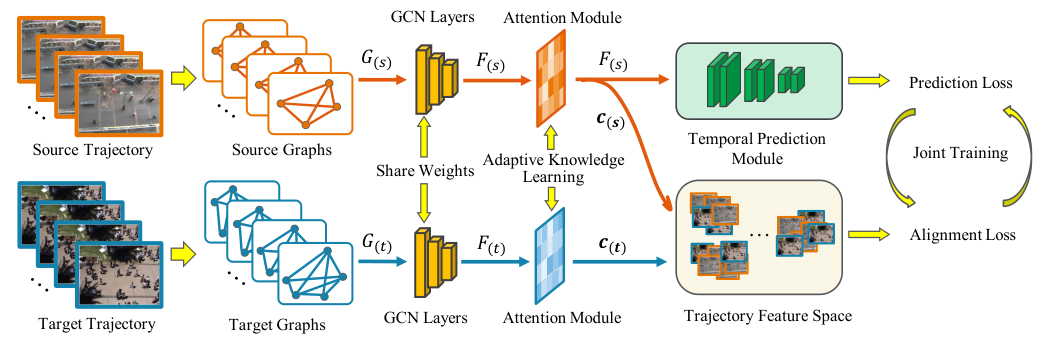
The overall framework of T-GNN model is illustrated in Fig. 3. It consists of three main components: 1) a graph neural network to extract effective spatial-temporal features of pedestrians from both source and target trajectory domains, 2) an attention-based adaptive knowledge learning module to explore domain-invariant individual-level representations for transfer learning, 3) a temporal prediction module for future pedestrian trajectory predictions.
3.1 Problem Definition
Given one pedestrian observed trajectory from time step to , aim to predict the future trajectory from time step to , where denote the coordinates. Considering all the pedestrians in the scene, the goal is to predict trajectories of all the pedestrians simultaneously by a model with parameter . Formally,
| (1) |
where is the set of future trajectories of all the pedestrians, denotes the number of pedestrians, and represents the collection of learnable parameters in the model.
3.2 Spatial-Temporal Feature Representations
Different from traditional time series forecasting, it is more challenging to predict pedestrian future trajectories because of the implicit human-human interactions and their strong temporal correlations. Therefore, extracting comprehensive spatial-temporal feature representations of observed pedestrian trajectories becomes a key point to accurately predict trajectories. In our work, considering the data structure of trajectories, a graph neural network is first employed to extract spatial-temporal feature representations.
Before constructing the graph, coordinates of all pedestrians are firstly passed through one layer as,
| (2) |
where is the number of pedestrians in the scene, represents the coordinates of pedestrian at the last observed frame . This decentralization operation is able to eliminate the effects of scene size differences and is also applied in recent works zhu2019starnet; xu2021tra2tra. We refer to as the “relative coordinates” for the following graph construction.
We define the graph , where is the vertex set of pedestrians in the graph, is the edge set that indicates the relationship between two pedestrians, and is the feature matrix associated with each pedestrian ( is the feature dimension). The topological structure of graph is represented by the adjacency matrix . In our case, the value of in adjacency matrix is initialized as the distance between pedestrian and as,
| (3) |
where is the distance, and denotes the “relative coordinates” of pedestrian at time step . As it should be other possible definitions of , we additionally investigate and analysis other three different definitions of , and results indicate that using distance is more appropriate in this situation.
The value of in feature matrix is defined as,
| (4) |
where are projection learnable parameters, is non-linearity activation function.
To measure the relative importance of dynamic spatial relations between pedestrians, the graph attention layer from velivckovic2017graph is adopted here to update the adjacency matrix . The graph attention coefficients are calculated as,
| (5) |
where is column vector in , are learnable parameters, represents the concatenation that operates in the dimension of row, is non-linearity activation function with . The same parameters are used here, see velivckovic2017graph for details.
The linear combination is thus computed according to the obtained attention coefficients. Formally, we have,
| (6) |
With each column vector concatenated together, we obtain the new updated adjacency matrix , which contains the information of global spatial features of pedestrians at time step . Then, the GCN layers kipf2016semi are applied here to further extract spatial-temporal features. Similar with mohamed2020social, we first add identity matrix to as,
| (7) |
Then, we stack from time step to as and also stack vertex feature matrices of the layer from time step to as , where represents the observation length. In addition, the stack of node degree matrices are correspondingly calculated from .
Finally, the output of the layer is calculated as,
| (8) |
where are learnable parameters of the layer.
In our case, three cascaded GCN layers () are employed to extract spatial-temporal feature representations of observed trajectories. Both source and target trajectories are constructed as graphs accordingly and then fed into the parameter-shared GCN layers for feature representation extraction. For simplicity, we denote the final feature representations of source trajectory domain as , and target trajectory domain as , where and are two different numbers of pedestrians from source and target domains.
3.3 Attention-Based Adaptive Learning
Given the misalignment of feature representations between source and target trajectory domains, we introduce an individual-wise attention-based adaptive knowledge learning module for transfer learning. Different from conventional domain adaptation situations, where each sample has determined category and fixed feature space. The feature space of trajectory sample is not fixed as the numbers of pedestrians are different in source and target trajectory domains. In order to address this misalignment problem, we propose a novel attention-based adaptive knowledge learning module to refine and effectively concentrate on the most relevant feature space for misalignment alleviation.
For individual-wise attention, we first reformat the final feature representations and as,
| (9) | ||||
where and correspond to the feature maps of one pedestrian from source and target trajectory domain. Then we reshape the feature maps and to the feature vector with the size of , where .
Although the feature vector keeps the spatial-temporal information of one pedestrian, we cannot decide how representative of one pedestrian’s feature vector is in one trajectory domain. Therefore, an attention module is introduced to learn the relative relevance between feature vectors and trajectory domain. The attention scores are calculated as,
| (10) | ||||
where and are learnable parameters. Then the final feature representations of source and target trajectory domains and are calculated as,
| (11) | ||||
These two context vectors and correspond to the refined individual-level representations of source and target trajectory domains. A similarity loss for distribution alignment is accordingly introduced as,
| (12) |
There are multiple choices for the distance function such as distance, MMD loss Ni2013Subspace; Long2015Learning, CORAL loss Sun2016Deep; Zhuo2017Deep, and adversarial loss Ganin2014Unsupervised; 2020Unsupervised. We explore these four alignment measures in Section 4, and results indicate that distance is more appropriate. Thus, we have,
| (13) |
3.4 Temporal Prediction Module
Instead of making predictions frame by frame, TCN GCRNSM2018Shaojie layers are employed to make future trajectory predictions based on the spatial-temporal feature representations from source trajectory domain. This prediction strategy is able to alleviate the error accumulating problem in sequential predictions caused by RNNs. It can also avoid gradient vanishing or reduce high computational costs hochreiter1997long; chung2014empirical. Recent works mohamed2020social; shi2021sgcn also utilized this strategy for prediction.
Given the feature representation , we pass through TCN layers in time dimension to obtain their corresponding future trajectories. Formally, for the TCN layer, we have,
| (14) |
where are leanable parameters of the TCN layer, represents the prediction output ( represents the length to be predicted). In our case, three three cascaded TCN layers () are employed to obtain the final output which we refer to as .
Similar assumption is made that pedestrian coordinates follow a bi-variate Gaussian distribution as , where is the mean, is the standard deviation, and is the correlation coefficient. These parameters are determined by passing through one linear layer as,
| (15) |
where are learnable parameters of this linear layer.
3.5 Objective Function
The overall objective function consists of two terms, the prediction loss for predicting future trajectory prediction and the alignment loss for aligning the distributions of source and target trajectory domains. The prediction loss is the negative log-likelihood as,
| (16) |
Note that only samples from source trajectory domain participate in the prediction phase. The whole model is trained by jointly minimizing the prediction loss and the alignment loss , thus we have,
| (17) |
where is a hyper-parameter for balancing these two terms.
4 Experiments
| Method | Year | Performance (ADE) (Source2Target) | Ave | |||||||||||||||||||
|---|---|---|---|---|---|---|---|---|---|---|---|---|---|---|---|---|---|---|---|---|---|---|
| A2B | A2C | A2D | A2E | B2A | B2C | B2D | B2E | C2A | C2B | C2D | C2E | D2A | D2B | D2C | D2E | E2A | E2B | E2C | E2D | |||
| Social-STGCNN mohamed2020social | 2020 | 1.83 | 1.58 | 1.30 | 1.31 | 3.02 | 1.38 | 2.63 | 1.58 | 1.16 | 0.70 | 0.82 | 0.54 | 1.04 | 1.05 | 0.73 | 0.47 | 0.98 | 1.09 | 0.74 | 0.50 | 1.22 |
| PECNet Mangalam2020It | 2020 | 1.97 | 1.68 | 1.24 | 1.35 | 3.11 | 1.35 | 2.69 | 1.62 | 1.39 | 0.82 | 0.93 | 0.57 | 1.10 | 1.17 | 0.92 | 0.52 | 1.01 | 1.25 | 0.83 | 0.61 | 1.31 |
| RSBG sun2020recursive | 2020 | 2.21 | 1.59 | 1.48 | 1.42 | 3.18 | 1.49 | 2.72 | 1.73 | 1.23 | 0.87 | 1.04 | 0.60 | 1.19 | 1.21 | 0.80 | 0.49 | 1.09 | 1.37 | 1.03 | 0.78 | 1.38 |
| Tra2Tra xu2021tra2tra | 2021 | 1.72 | 1.58 | 1.27 | 1.37 | 3.32 | 1.36 | 2.67 | 1.58 | 1.16 | 0.70 | 0.85 | 0.60 | 1.09 | 1.07 | 0.81 | 0.52 | 1.03 | 1.10 | 0.75 | 0.52 | 1.25 |
| SGCN shi2021sgcn | 2021 | 1.68 | 1.54 | 1.26 | 1.28 | 3.22 | 1.38 | 2.62 | 1.58 | 1.14 | 0.70 | 0.82 | 0.52 | 1.05 | 0.97 | 0.80 | 0.48 | 0.97 | 1.08 | 0.75 | 0.51 | 1.22 |
| T-GNN (Ours) | - | 1.13 | 1.25 | 0.94 | 1.03 | 2.54 | 1.08 | 2.25 | 1.41 | 0.97 | 0.54 | 0.61 | 0.23 | 0.88 | 0.78 | 0.59 | 0.32 | 0.87 | 0.72 | 0.65 | 0.34 | 0.96 |
| Method | Year | Performance (FDE) (Source2Target) | Ave | |||||||||||||||||||
|---|---|---|---|---|---|---|---|---|---|---|---|---|---|---|---|---|---|---|---|---|---|---|
| A2B | A2C | A2D | A2E | B2A | B2C | B2D | B2E | C2A | C2B | C2D | C2E | D2A | D2B | D2C | D2E | E2A | E2B | E2C | E2D | |||
| Social-STGCNN mohamed2020social | 2020 | 3.24 | 2.86 | 2.53 | 2.43 | 5.16 | 2.51 | 4.86 | 2.88 | 2.30 | 1.34 | 1.74 | 1.10 | 2.21 | 1.99 | 1.41 | 0.88 | 2.10 | 2.05 | 1.47 | 1.01 | 2.30 |
| PECNet Mangalam2020It | 2020 | 3.33 | 2.83 | 2.53 | 2.45 | 5.23 | 2.48 | 4.90 | 2.86 | 2.22 | 1.32 | 1.68 | 1.12 | 2.20 | 2.05 | 1.52 | 0.88 | 2.10 | 1.84 | 1.45 | 0.98 | 2.29 |
| RSBG sun2020recursive | 2020 | 3.42 | 2.96 | 2.75 | 2.50 | 5.28 | 2.59 | 5.19 | 3.10 | 2.36 | 1.55 | 1.99 | 1.37 | 2.28 | 2.22 | 1.77 | 0.97 | 2.19 | 2.29 | 1.81 | 1.34 | 2.50 |
| Tra2Tra xu2021tra2tra | 2021 | 3.29 | 2.88 | 2.66 | 2.45 | 5.22 | 2.50 | 4.89 | 2.90 | 2.29 | 1.33 | 1.78 | 1.09 | 2.26 | 2.12 | 1.63 | 0.92 | 2.18 | 2.06 | 1.52 | 1.17 | 2.34 |
| SGCN shi2021sgcn | 2021 | 3.22 | 2.81 | 2.52 | 2.40 | 5.18 | 2.47 | 4.83 | 2.85 | 2.24 | 1.32 | 1.71 | 1.03 | 2.23 | 1.90 | 1.48 | 0.97 | 2.10 | 1.95 | 1.52 | 0.99 | 2.29 |
| T-GNN (Ours) | - | 2.18 | 2.25 | 1.78 | 1.84 | 4.15 | 1.82 | 4.04 | 2.53 | 1.91 | 1.12 | 1.30 | 0.87 | 1.92 | 1.46 | 1.25 | 0.65 | 1.86 | 1.45 | 1.28 | 0.72 | 1.82 |
| Method | Average Performance |
|---|---|
| ADE/FDE | |
| T-GNN+MMD Long2015Learning | 1.11/2.11 |
| T-GNN+CORAL Zhuo2017Deep | 1.07/2.01 |
| T-GNN+GFK 2015Geodesic | 1.15/2.08 |
| T-GNN+UDA 2020Unsupervised | 1.07/2.09 |
| T-GNN (Ours) | 0.96/1.82 |
| Value | |||||
|---|---|---|---|---|---|
| ADE | 1.19 | 1.05 | 0.96 | 1.16 | 1.31 |
| FDE | 2.16 | 2.02 | 1.82 | 2.07 | 2.45 |
In this section, we first present the definition of our proposed new setting as well as the evaluation protocol, then we carry out extensive evaluations on our proposed T-GNN model under this new setting, in comparison with previous existing methods and different domain adaptation strategies. Additional evaluation results and feature visualizations are provided in the supplementary material.
Datasets. Experiments are conducted on two real-world datasets: ETH Pellegrini2009You and UCY Lerner2010Crowds as these two public datasets are widely used in this task. ETH consists of two scenes named ETH and HOTEL, and UCY consists of three scenes named UNIV, ZARA1, and ZARA2.
Experimental Setting. We introduce a more general and practical setting that treats each scene as one trajectory domain. The model is trained on only one domain and tested on other four domains, respectively. Given five trajectory domains, we have total 20 trajectory prediction tasks: A B/C/D/E, B A/C/D/E, C A/B/D/E, D A/B/C/E, and E A/B/C/D, where A, B, C, D, and E represents ETH, HOTEL, UNIV, ZARA1, and ZARA2, respectively. This setting is challenging because of the domain gap issue.
Evaluation Protocol. To ensure the fair comparison under the new setting, existing baselines are trained with one source trajectory domain as well as the validation set of the target trajectory domain. Specifically, take A B as the example, existing baselines are trained with the training set of A and the validation set of B, then evaluated on the testing set of B. Our proposed model considers the training set of A as the source trajectory domain and the validation set of B as the target trajectory domain, then evaluated on the testing set of B. Note that the validation set and the testing set are independent of each other and there is no overlap sample between the validation set and the testing set. In the training phase, our proposed model only has access to the observed trajectory from the validation set.
Baselines. Five state-of-the-art methods are compared with our proposed method under the new setting and the evaluation protocol. Social-STGCNN mohamed2020social, PECNet Mangalam2020It, RSBG sun2020recursive, SGCN shi2021sgcn, and Tra2Tra xu2021tra2tra. We also use following four widely-used DA approaches for comparison. T-GNN+MMD: using the multi kernel-maximum mean discrepancies loss Long2015Learning as , T-GNN+CORAL: using the CORAL loss Sun2016Deep as ; T-GNN+GFK: using the kernel-based domain adaptation strategy 2015Geodesic, and T-GNN+UDA: unsupervised domain adaptive graph convolutional network using the adversarial loss 2020Unsupervised.
Evaluation Metrics. Following two metrics are used to for performance evaluation. In these two metrics, is the total number of pedestrians in target trajectory domain, are predictions, and are ground-truth coordinates.
- •
Average Displacement Error (ADE):
(18) - •
Final Displacement Error (FDE):
(19)
Implementation Details. Similar with previous baselines, 8 frames are observed and the next 12 frames are predicted. The number of GCN layers is set as 3, the number of TCN layers is set as 3, and the feature dimension is set as 64. In the training phase, the batch size is set as 16 and is set as 1. The whole model is trained for 200 epochs and Adam diederik2015adam is applied as the optimizer. We set the initial learning rate as 0.001 and change to 0.0005 after 100 epochs. In the inference phase, 20 predicted trajectories are sampled and the best amongst 20 predictions is used for evaluation.
| Variants | ID | Performance (ADE/FDE) | ||||
|---|---|---|---|---|---|---|
| A2B | B2C | C2D | D2E | E2A | ||
| T-GNN w/o GAL | 1 | 1.51/2.34 | 1.17/1.90 | 0.69/1.42 | 0.39/0.71 | 0.90/1.98 |
| T-GNN w/o AAL w/ AP | 2 | 1.78/2.85 | 1.23/2.02 | 0.77/1.53 | 0.42/0.79 | 0.96/2.03 |
| T-GNN w/o AAL w/ LL | 3 | 1.81/2.91 | 1.25/2.03 | 0.76/1.48 | 0.43/0.79 | 0.94/2.01 |
| Social-STGCNN- mohamed2020social | 4 | 2.18/3.68 | 2.30/3.21 | 1.59/2.54 | 1.23/1.72 | 1.73/2.98 |
| SGCN- shi2021sgcn | 5 | 2.03/3.53 | 2.35/3.22 | 1.68/2.71 | 1.12/1.59 | 1.81/3.02 |
| T-GNN- | 6 | 2.12/3.58 | 2.28/3.21 | 1.73/2.76 | 1.19/1.58 | 1.74/2.95 |
| Social-STGCNN mohamed2020social | 7 | 1.83/3.24 | 1.38/2.51 | 0.82/1.74 | 0.47/0.88 | 0.98/2.10 |
| SGCN shi2021sgcn | 8 | 1.68/3.24 | 1.38/2.47 | 0.82/1.71 | 0.48/0.97 | 0.97/2.10 |
| T-GNN- | 9 | 1.89/3.25 | 1.35/2.48 | 0.88/1.93 | 0.53/0.97 | 0.98/2.16 |
| T-GNN (Ours) | 10 | 1.13/2.18 | 1.08/1.82 | 0.61/1.30 | 0.32/0.65 | 0.87/1.86 |
4.1 Quantitative Analysis
Tables 2 and 3 show the evaluation results of 20 tasks in comparison with five existing baselines. Table 4 shows the average performance of total 20 tasks in comparison with four existing domain adaptation approaches.
T-GNN vs Other Baselines. In general, our proposed T-GNN model, no matter on which task, consistently outperforms the other five baselines. Overall, our T-GNN model improves by comparing with Social-STGCNN and SGCN models on the ADE metric, and improves by comparing with PCENet and SGCN models on the FDE metric. It validates that our T-GNN model has the ability to learn transferable knowledge from source to target trajectory domain and alleviate the domain gap. As mentioned in Section 4, these baselines have access to the whole validation set of the target domain while our model only has access to the observed trajectories from the validation set. Results indicate that directly training with mixed data from different trajectory domains is worse than with our domain-invariant knowledge learning approach. In addition, for tasks D2E and E2D, all the models have relatively smaller ADE and FDE. One possible reason is that domain D (ZARA1) and E (ZARA2) have similar background and surroundings, in which pedestrians may have similar moving pattern. This phenomenon further illustrates the importance of considering the domain-shift problem in trajectory prediction task.
T-GNN vs Other DA Approaches11 1 Performance of total 20 tasks and the implementation details of T-GNN+UDA model are provided in supplementary material since T-GNN+UDA uses an adversarial loss.. Generally speaking, our T-GNN model using distance as the alignment loss achieves the best average performance. It indicates that distance is more appropriate for similarity measure in trajectory prediction task. One intuitive reason is that in trajectory prediction task, high-dimensional feature representations may still reserve the spatial-level information.
4.2 Ablation Study
We first study the performance of different values of in the objective function, and then study the contributions of each proposed component. In addition, we investigate the functionality of our proposed adaptive learning module.
Performance Study of . The hyper-parameter is used to balance the two terms in Eq. 17. Setting too small results in the failure of alignment, on the contrary, setting too large results in too heavy alignment. We set different values to find the most suitable . Table 5 shows the average performance on 20 tasks of our T-GNN model with five different values . When we set , our T-GNN model can achieve the best performance.
Contributions of Each Component. We evaluate following 3 different variants of our T-GNN model on 5 selected tasks A2B, B2C, C2D, D2E, and E2A. (1) T-GNN w/o GAL denotes that the graph attention component defined in Eqs. 5 and 6 is removed, thus will not be updated during training. (2) T-GNN w/o AAL w/ AP denotes that the attention-based adaptive learning module is replaced with one average pooling layer, in which features and are reshaped and passed through one average pooling layer that operates in the “sample” dimension to obtain and . (3) T-GNN w/o AAL w/ LL denotes that the attention-based adaptive learning module is replaced with one trainable linear layer. The results are illustrated in Table 6.
It can be observed from Table 6 that removing the graph attention component results in the performance reduction, which indicates the graph attention component is effective to extract relation features. Replacing our proposed attention-based adaptive learning module with either one average pooling layer or one trainable linear layer also results in the performance reduction, which indicates the effectiveness of our proposed adaptive learning module for exploring the individual-level domain-invariant knowledge.
Effectiveness of Adaptive Learning. Experiments are carried out to further study the effectiveness of adaptive learning module in our T-GNN model. We remove the attention-based adaptive learning module presented in Section 3.3 and disregard the alignment loss defined in Eq. 13. Thus, our model is trained only on the source trajectory domain and evaluated on one novel target trajectory domain, which we refer to as T-GNN-. For further comparison, two graph-based baselines Social-STGCNN mohamed2020social and SGCN shi2021sgcn are also trained without using the validation set, which we refer to as Social-STGCNN- and SGCN-. In addition, we directly train our model with mixed samples without domain-invariant adaptive learning module, which we refer to as T-GNN-. The results are illustrated in Table 6.
In comparison with variants 4, 5, and 6, the results indicate that the backbone of our T-GNN model is competitive with these two graph-based backbones, which validates that our T-GNN can extract effective spatial-temporal features of observed trajectories. In comparison with variants 7, 8, and 9, all three variants can achieve competitive performance since the training data is exactly the same. In addition, these three variants all outperform variants 4, 5, and 6 correspondingly, because variants 7, 8, and 9 all have access to the validation set of target trajectory domain. Results of variants 7, 8, 9 and 10 validate that our proposed domain-invariant transfer learning approach is superior to directly training with mixed data from different trajectory domains.
5 Conclusion
In this paper, we delve into the domain shift challenge in the pedestrian trajectory prediction task. Specifically, a more real, practical yet challenging trajectory prediction setting is proposed. Then we propose a unified model which contains a Transferable Graph Neural Network for future trajectory prediction as well as a domain-invariant knowledge learning approach simultaneously. Extensive experiments prove the superiority of our T-GNN model in both future trajectory prediction and trajectory domain-shift alleviation. Our work is the first that studies this problem and fills the gap in benchmarks and techniques for practical pedestrian trajectory prediction across different domains.
Supplementary Material
6 Overview
In the supplementary material, we provide experimental details and more evaluation results including visualizations. We also provide our insights and discussions at the end.
7 Experiments
7.1 Dataset Details
There are two commonly used datasets including five scenes in our work: ETH22 2 http://www.vision.ee.ethz.ch/en/datasets/. Pellegrini2009You and UCY33 3 https://graphics.cs.ucy.ac.cy/research/downloads/crowd-data. Lerner2010Crowds. Dataset ETH consists of two scenes: ETH and HOTEL. Dataset UCY consists of three scenes: UNIV, ZARA1, and ZARA2. Each scene contains multiple walking pedestrians with different complex walking motions. We show examples of each scene in Fig. 4 with one red dot as one person. Some basic information of two datasets is shown in Table 7, additional statistics of five scenes have been provided in the main body.


| Dataset | Year | Location | Target | Sensors | Description | Duration and tracks | Annotations | Sampling |
|---|---|---|---|---|---|---|---|---|
| ETH | 2009 | Outdoor | People | Camera/Top-down view | Two scenes | 25 min, 650 tracks | Positions, velocities, groups, maps | @2.5Hz |
| UCY | 2007 | Outdoor | People | Camera/Top-down view | Three scenes | 16.5 min, over 700 tracks | Positions, gaze directions |
7.2 Implementation Details
We compare our proposed model with total 5 trajectory prediction baselines: Social-STGCNN mohamed2020social,
PECNet Mangalam2020It, RSBG sun2020recursive, SGCN shi2021sgcn, and Tra2Tra xu2021tra2tra. We implemented these baselines with their provided codes: Social-STGCNN 44
4
https://github.com/abduallahmohamed/Social-STGCNN., PECNet 55
5
https://github.com/HarshayuGirase/Human-Path-Prediction., SGCN 66
6
https://github.com/shuaishiliu/SGCN.. We tried our best to reproduce the codes of RSBG and authors have shared the codes of Tra2Tra with us.We also employ 4 domain adaptation approaches: T-GNN+MMD Long2015Learning , T-GNN+CORAL Sun2016Deep, T-GNN+GFK 2015Geodesic, and T-GNN+UDA 2020Unsupervised. We implemented these approaches based on the codes: MMD 77
7
https://github.com/easezyc/deep-transfer-learning., CORAL88
8
https://github.com/VisionLearningGroup/CORAL., GFK 99
9
https://github.com/jindongwang/transferlearning/tree/master/code/
traditional/GFK., UDA 1010
10
https://github.com/GRAND-Lab/UDAGCN..
7.3 Performance Study of
As mentioned in the main body, the value of in adjacency matrix is initialized as the distance between pedestrian and ,
| (20) |
where is the distance, and denotes the “relative coordinates” of pedestrian at time step .
As it should be other possible definitions of , thus we investigate and analysis different definitions of as follows. Among these different functions, the key starting point we follow is that could be the function of the relative coordinates of pedestrians and . Average ADE and FDE results are shown in Table 8.
| (21) | ||||
| (22) | ||||
| (23) |
where and are both two small positive constants to ensure the numerical stability. In real practice, it is really difficult to have and we set though.
| Variants | Performance | |
|---|---|---|
| ADE | FDE | |
| 1.03 | 1.99 | |
| () | 1.17 | 2.10 |
| () | 1.09 | 1.99 |
| () | 1.14 | 2.07 |
| 1.08 | 1.92 | |
| 0.96 | 1.82 | |
7.4 Results of Other DA Approaches
| Metric | Method | Performance (Source2Target) | Ave | |||||||||||||||||||
|---|---|---|---|---|---|---|---|---|---|---|---|---|---|---|---|---|---|---|---|---|---|---|
| A2B | A2C | A2D | A2E | B2A | B2C | B2D | B2E | C2A | C2B | C2D | C2E | D2A | D2B | D2C | D2E | E2A | E2B | E2C | E2D | |||
| ADE | T-GNN+MMD Long2015Learning | 1.53 | 1.39 | 1.14 | 1.19 | 2.99 | 1.18 | 2.39 | 1.49 | 1.08 | 0.62 | 0.71 | 0.42 | 1.02 | 0.89 | 0.68 | 0.38 | 0.89 | 0.99 | 0.74 | 0.41 | 1.11 |
| T-GNN+CORAL Zhuo2017Deep | 1.43 | 1.35 | 1.09 | 1.12 | 2.87 | 1.12 | 2.31 | 1.46 | 1.03 | 0.58 | 0.68 | 0.46 | 0.99 | 0.85 | 0.66 | 0.40 | 0.86 | 0.96 | 0.67 | 0.41 | 1.07 | |
| T-GNN+GFK 2015Geodesic | 1.69 | 1.52 | 1.20 | 1.24 | 3.01 | 1.19 | 2.52 | 1.55 | 1.11 | 0.68 | 0.69 | 0.50 | 0.96 | 0.89 | 0.71 | 0.43 | 0.89 | 1.01 | 0.75 | 0.42 | 1.15 | |
| T-GNN+UDA 2020Unsupervised | 1.41 | 1.32 | 0.98 | 1.23 | 2.92 | 1.20 | 2.43 | 1.42 | 1.12 | 0.64 | 0.62 | 0.48 | 0.91 | 0.81 | 0.69 | 0.35 | 0.91 | 0.98 | 0.70 | 0.39 | 1.07 | |
| T-GNN (Ours) | 1.13 | 1.25 | 0.94 | 1.03 | 2.54 | 1.08 | 2.25 | 1.41 | 0.97 | 0.54 | 0.61 | 0.23 | 0.88 | 0.78 | 0.59 | 0.32 | 0.87 | 0.72 | 0.65 | 0.34 | 0.96 | |
| FDE | T-GNN+MMD Long2015Learning | 2.63 | 2.65 | 1.98 | 2.24 | 4.86 | 2.15 | 4.63 | 2.69 | 2.16 | 1.25 | 1.52 | 0.99 | 2.20 | 1.88 | 1.39 | 0.75 | 2.03 | 1.84 | 1.46 | 0.82 | 2.11 |
| T-GNN+CORAL Zhuo2017Deep | 2.44 | 2.52 | 1.82 | 2.16 | 4.59 | 1.89 | 4.48 | 2.68 | 2.09 | 1.20 | 1.47 | 0.97 | 2.09 | 1.83 | 1.33 | 0.75 | 2.01 | 1.79 | 1.38 | 0.79 | 2.01 | |
| T-GNN+GFK 2015Geodesic | 2.67 | 2.66 | 2.03 | 2.21 | 4.74 | 2.12 | 4.88 | 2.68 | 2.19 | 1.23 | 1.34 | 1.01 | 1.96 | 1.77 | 1.30 | 0.76 | 2.03 | 1.83 | 1.43 | 0.78 | 2.08 | |
| T-GNN+UDA 2020Unsupervised | 2.59 | 2.61 | 1.94 | 2.25 | 4.81 | 2.13 | 4.85 | 2.63 | 2.19 | 1.29 | 1.42 | 1.03 | 2.03 | 1.75 | 1.37 | 0.73 | 2.08 | 1.80 | 1.45 | 0.76 | 2.09 | |
| T-GNN (Ours) | 2.18 | 2.25 | 1.78 | 1.84 | 4.15 | 1.82 | 4.04 | 2.53 | 1.91 | 1.12 | 1.30 | 0.87 | 1.92 | 1.46 | 1.25 | 0.65 | 1.86 | 1.45 | 1.28 | 0.72 | 1.82 | |
Table 9 shows evaluation results of total 20 tasks when comparing with other domain adaptation approaches. For model T-GNN+UDA, in which there is an adversarial loss that measured by an extra domain classifier. One fully-connected linear layer is employed as the classifier. In specific, this kind of models needs to minimize the adversarial loss with respect to parameters of domain classifier, while maximizing it with respect to the parameters of trajectory predictor. Thus we use a a gradient reversal layer ganin2015unsupervised for the min-max optimization to unify the training procedure in a single step. It can be observed that our proposed adaptive learning module outperforms these domain adaptation approaches. This may show that our designed alignment loss is more appropriate for adapting fine-grained individual-level features in trajectory prediction task.
7.5 t-SNE Visualization


In this section, we visualize feature representations and of the target and source trajectory domain with t-SNE 2008Visualizing approach on of 4 tasks. Fig. 5 shows the visualization examples where red and blue denote the source and target trajectory features, respectively. The first row are and without attention-based adaptive learning module , which we denote as “w/o AAL” (corresponding to the Variant T-GNN- in the main body). The second row are with attention-based adaptive learning module, which we denote as “w AAL”. Each dot represents the feature of one pedestrian in the figure. Different from conventional t-SNE visualizations that applied in classification task, there is no specific “label” of each dot in our task. Therefore, the cluster structure may not be clear in our task.
For task BD and CE, we can observe that features get closer with our adaptive learning module, which validates that our proposed adaptation learning module is able to alleviate the disparities across different trajectory domains. In addition, the visualization of task BD is not significant and the corresponding quantitative results of task is BD lower than others (ADE: 2.25, FDE:4.04). For task DE and ED, since D (ZARA1) and E (ZARA2) have similar scenes, we can observe from these two pairs of figures: (1) features from source and target domains have more overlaps, (2) features become more closer. It is consistent with their corresponding quantitative results (DE: 0.32/0.65, ED: 0.34/0.72). It also validates the effectiveness of our proposed adaptive learning module.
8 Discussion
Compare with general domain adaptation methods. We delve into the domain-shift challenge in the task of pedestrian trajectory prediction in this paper. In image/video-related classification tasks, domain adaptation (DA) is a hot topic that aims to enable models to generate to novel datasets with different sample distributions. In this study, we expose the challenging domain-shift issue in future trajectory prediction. We usually consider the trajectory as two parts: observation and prediction. It is different from conventional DA tasks where data is in the form of sample-label pairs. Strictly speaking, in trajectory prediction task, the prediction part is not exactly the “label” of the observation part. This essential difference brings in another interesting finding that is worth exploring. In Fig. 5, the cluster structure is not clear because there is no category of each trajectory, which means there exists distribution overlap of different trajectory domains. This kind of “overlap” may be reason of the variance of different tasks. If this “overlap” problem as well as domain-shift problem can be well-addressed simultaneously, trajectory prediction task would be more practical and promising. On the other hand, the observation and prediction parts of one trajectory are totally consistent, thus these two parts may be able to swap and supervise each other. We hope this perspective will inspire the research communities of considering the trajectory prediction problem as well as domain shift issue.
References
- (1) Alexandre Alahi, Kratarth Goel, Vignesh Ramanathan, Alexandre Robicquet, Li Fei-Fei, and Silvio Savarese. Social LSTM: Human trajectory prediction in crowded spaces. In Proceedings of the IEEE Conference on Computer Vision and Pattern Recognition, pages 961–971, 2016.
- (2) Javad Amirian, Jean-Bernard Hayet, and Julien Pettré. Social ways: Learning multi-modal distributions of pedestrian trajectories with GANs. In Proceedings of the IEEE Conference on Computer Vision and Pattern Recognition Workshops, pages 2964–2972, 2019.
- (3) Haoyu Bai, Shaojun Cai, Nan Ye, David Hsu, and Wee Sun Lee. Intention-aware online POMDP planning for autonomous driving in a crowd. In Proceedings of the IEEE International Conference on Robotics and Automation, pages 454–460, 2015.
- (4) Shaojie Bai, J. Zico Kolter, and Vladlen Koltun. An empirical evaluation of generic convolutional and recurrent networks for sequence modeling. arXiv:1803.01271, 2018.
- (5) Niccoló Bisagno, Bo Zhang, and Nicola Conci. Group LSTM: Group trajectory prediction in crowded scenarios. In Proceedings of the European Conference on Computer Vision, pages 213–225, 2018.
- (6) Ruichu Cai, Fengzhu Wu, Zijian Li, Pengfei Wei, Lingling Yi, and Kun Zhang. Graph domain adaptation: A generative view. arXiv preprint arXiv:2106.07482, 2021.
- (7) Guangyi Chen, Junlong Li, Jiwen Lu, and Jie Zhou. Human trajectory prediction via counterfactual analysis. In Proceedings of the IEEE International Conference on Computer Vision, pages 9824–9833, 2021.
- (8) Guangyi Chen, Junlong Li, Nuoxing Zhou, Liangliang Ren, and Jiwen Lu. Personalized trajectory prediction via distribution discrimination. In Proceedings of the IEEE International Conference on Computer Vision, pages 15580–15589, 2021.
- (9) Hao Cheng, Wentong Liao, Xuejiao Tang, Michael Ying Yang, Monika Sester, and Bodo Rosenhahn. Exploring dynamic context for multi-path trajectory prediction. arXiv preprint arXiv:2010.16267, 2020.
- (10) Junyoung Chung, Caglar Gulcehre, KyungHyun Cho, and Yoshua Bengio. Empirical evaluation of gated recurrent neural networks on sequence modeling. arXiv preprint arXiv:1412.3555, 2014.
- (11) Patrick Dendorfer, Sven Elflein, and Laura Leal-Taixé. Mg-gan: A multi-generator model preventing out-of-distribution samples in pedestrian trajectory prediction. In Proceedings of the IEEE International Conference on Computer Vision, pages 13158–13167, 2021.
- (12) Jacob Devlin, Ming Wei Chang, Kenton Lee, and Kristina Toutanova. BERT: Pre-training of deep bidirectional transformers for language understanding. arXiv preprint arXiv:1810.04805, 2018.
- (13) P. Kingma Diederik and Ba Jimmy. Adam: A method for stochastic optimization. In Proceedings of the International Conference on Learning Representations, 2015.
- (14) Zhengming Ding, Sheng Li, Ming Shao, and Yun Fu. Graph adaptive knowledge transfer for unsupervised domain adaptation. In Proceedings of the European Conference on Computer Vision, pages 37–52, 2018.
- (15) David Ellis, Eric Sommerlade, and Ian Reid. Modelling pedestrian trajectory patterns with gaussian processes. In Proceedings of the IEEE International Conference on Computer Vision Workshops, pages 1229–1234, 2009.
- (16) Tharindu Fernando, Simon Denman, Sridha Sridharan, and Clinton Fookes. GD-GAN: Generative adversarial networks for trajectory prediction and group detection in crowds. In Proceedings of the Asian Conference on Computer Vision, pages 314–330, 2018.
- (17) Yaroslav Ganin and Victor Lempitsky. Unsupervised domain adaptation by backpropagation. In Proceedings of the International Conference on Machine Learning, pages 1180–1189, 2015.
- (18) Yaroslav Ganin and Victor Lempitsky. Unsupervised domain adaptation by backpropagation. In Proceedings of the International Conference on Machine Learning, pages 1180–1189. PMLR, 2015.
- (19) Jiyang Gao, Chen Sun, Hang Zhao, Yi Shen, Dragomir Anguelov, Congcong Li, and Cordelia Schmid. VectorNet: Encoding HD maps and agent dynamics from vectorized representation. In Proceedings of the IEEE Conference on Computer Vision and Pattern Recognition, pages 11522–11530, 2020.
- (20) Francesco Giuliari, Irtiza Hasan, Marco Cristani, and Fabio Galasso. Transformer networks for trajectory forecasting. In Proceedings of the IEEE International Conference on Pattern Recognition, pages 10335–10342, 2020.
- (21) Boqing Gong, Yuan Shi, Fei Sha, and K. Grauman. Geodesic flow kernel for unsupervised domain adaptation. In Proceedings of the IEEE Conference on Computer Vision and Pattern Recognition, pages 2066–2073, 2015.
- (22) Agrim Gupta, Justin Johnson, Li Fei-Fei, Silvio Savarese, and Alexandre Alahi. Social GAN: Socially acceptable trajectories with generative adversarial networks. In Proceedings of the IEEE Conference on Computer Vision and Pattern Recognition, pages 2255–2264, 2018.
- (23) Gewen He, Xiaofeng Liu, Fangfang Fan, and Jane You. Classification-aware semi-supervised domain adaptation. In Proceedings of the IEEE Conference on Computer Vision and Pattern Recognition Workshops, pages 4147–4156, 2020.
- (24) Sepp Hochreiter and Jurgen Schmidhuber. Long short-term memory. Neural Computation, 9(8):1735–1780, 1997.
- (25) Yue Hu, Siheng Chen, Ya Zhang, and Xiao Gu. Collaborative motion prediction via neural motion message passing. In Proceedings of the IEEE Conference on Computer Vision and Pattern Recognition, pages 6319–6328, 2020.
- (26) Hal Daumé III, Abhishek Kumar, and Avishek Saha. Co-regularization based semi-supervised domain adaptation. In Proceedings of the Advances in Neural Information Processing Systems, 2010.
- (27) Boris Ivanovic and Marco Pavone. The trajectron: Probabilistic multi-agent trajectory modeling with dynamic spatiotemporal graphs. In Proceedings of the IEEE International Conference on Computer Vision, pages 2375–2384, 2019.
- (28) Ashesh Jain, Amir R Zamir, Silvio Savarese, and Ashutosh Saxena. Structural-RNN: Deep learning on spatio-temporal graphs. In Proceedings of the IEEE Conference on Computer Vision and Pattern Recognition, pages 5308–5317, 2016.
- (29) Magdiel Jiménez-Guarneros and Pilar Gómez-Gil. A study of the effects of negative transfer on deep unsupervised domain adaptation methods. Expert Systems with Applications, 167:114088, 2020.
- (30) Christopher Keat and Christian Laugier. Modelling smooth paths using gaussian processes. In Proceedings of the International Conference on Field and Service Robotics, pages 381–390, 2007.
- (31) Thomas N Kipf and Max Welling. Semi-supervised classification with graph convolutional networks. In Proceedings of the International Conference on Learning Representations, 2017.
- (32) Kris M. Kitani, Brian D. Ziebart, James Andrew Bagnell, and Martial Hebert. Activity forecasting. In Proceedings of the European Conference on Computer Vision, pages 201–214, 2012.
- (33) Vineet Kosaraju, Amir Sadeghian, Roberto Martín-Martín, Ian Reid, Hamid Rezatofighi, and Silvio Savarese. Social-bigat: Multimodal trajectory forecasting using bicycle-gan and graph attention networks. In Proceedings of the Advances in Neural Information Processing Systems, pages 137–146, 2019.
- (34) Parth Kothari, Brian Sifringer, and Alexandre Alahi. Interpretable social anchors for human trajectory forecasting in crowds. In Proceedings of the IEEE Conference on Computer Vision and Pattern Recognition, pages 15556–15566, 2021.
- (35) Van Der Maaten Laurens and Geoffrey Hinton. Visualizing data using t-SNE. Journal of Machine Learning Research, 9(2605):2579–2605, 2008.
- (36) Alon Lerner, Yiorgos Chrysanthou, and Dani Lischinski. Crowds by example. Computer Graphics Forum, 26(3):655–664, 2010.
- (37) Jiachen Li, Hengbo Ma, and Masayoshi Tomizuka. Conditional generative neural system for probabilistic trajectory prediction. arXiv preprint arXiv:1905.01631, 2019.
- (38) Shijie Li, Yanying Zhou, Jinhui Yi, and Juergen Gall. Spatial-temporal consistency network for low-latency trajectory forecasting. In Proceedings of the IEEE International Conference on Computer Vision, pages 1940–1949, 2021.
- (39) Junwei Liang, Lu Jiang, and Alexander Hauptmann. Simaug: Learning robust representations from simulation for trajectory prediction. In Proceedings of the European Conference on Computer Vision, pages 275–292, 2020.
- (40) Junwei Liang, Lu Jiang, Juan Carlos Niebles, Alexander G Hauptmann, and Li Fei-Fei. Peeking into the future: Predicting future person activities and locations in videos. In Proceedings of the IEEE Conference on Computer Vision and Pattern Recognition, pages 5725–5734, 2019.
- (41) Mingsheng Long, Yue Cao, Jianmin Wang, and Michael Jordan. Learning transferable features with deep adaptation networks. In Proceedings of the International Conference on Machine Learning, pages 97–105, 2015.
- (42) Matthias Luber, Johannes A Stork, Gian Diego Tipaldi, and Kai O Arras. People tracking with human motion predictions from social forces. In Proceedings of the IEEE International Conference on Robotics and Automation, pages 464–469, 2010.
- (43) Zimeng Luo, Jiani Hu, Weihong Deng, and Haifeng Shen. Deep unsupervised domain adaptation for face recognition. In Proceedings of the IEEE International Conference on Automatic Face & Gesture Recognition, pages 453–457, 2018.
- (44) Qianqian Ma, Yang-Yu Liu, and Alex Olshevsky. Optimal lockdown for pandemic control. arXiv preprint arXiv:2010.12923, 2020.
- (45) Qianqian Ma and Alex Olshevsky. Adversarial crowdsourcing through robust rank-one matrix completion. In Proceedings of the Advances in Neural Information Processing Systems, pages 21841–21852, 2020.
- (46) Osama Makansi, Özgün Cicek, Yassine Marrakchi, and Thomas Brox. On exposing the challenging long tail in future prediction of traffic actors. In Proceedings of the IEEE International Conference on Computer Vision, pages 13127–13137, 2021.
- (47) Dimitrios Makris and Tim Ellis. Spatial and probabilistic modelling of pedestrian behaviour. In Proceedings of the British Machine Vision Conference, pages 54.1–54.10, 2002.
- (48) Karttikeya Mangalam, Yang An, Harshayu Girase, and Jitendra Malik. From goals, waypoints & paths to long term human trajectory forecasting. In Proceedings of the IEEE International Conference on Computer Vision, pages 15233–15242, 2021.
- (49) Karttikeya Mangalam, Harshayu Girase, Shreyas Agarwal, Kuan Hui Lee, Ehsan Adeli, Jitendra Malik, and Adrien Gaidon. It is not the journey but the destination: Endpoint conditioned trajectory prediction. In Proceedings of the European Conference on Computer Vision, pages 759–776, 2020.
- (50) Abduallah Mohamed, Kun Qian, Mohamed Elhoseiny, and Christian Claudel. Social-STGCNN: A social spatio-temporal graph convolutional neural network for human trajectory prediction. In Proceedings of the IEEE Conference on Computer Vision and Pattern Recognition, pages 14424–14432, 2020.
- (51) Mehdi Moussaïd, Niriaska Perozo, Simon Garnier, Dirk Helbing, and Guy Theraulaz. The walking behaviour of pedestrian social groups and its impact on crowd dynamics. PloS one, 5(4):e10047, 2010.
- (52) Basam Musleh, Fernando García, Javier Otamendi, José Ma Armingol, and De La Escalera Arturo. Identifying and tracking pedestrians based on sensor fusion and motion stability predictions. Sensors, 10(9):8028–8053, 2010.
- (53) Jie Ni, Qiang Qiu, and Rama Chellappa. Subspace interpolation via dictionary learning for unsupervised domain adaptation. Proceedings of the IEEE Conference on Computer Vision and Pattern Recognition, pages 692–699, 2013.
- (54) Takenori Obo and Yuto Nakamura. Intelligent robot navigation based on human emotional model in human-aware environment. In Proceedings of the International Conference on Machine Learning and Cybernetics, pages 1–6, 2020.
- (55) Bo Pang, Tianyang Zhao, Xu Xie, and Ying Nian Wu. Trajectory prediction with latent belief energy-based model. In Proceedings of the IEEE Conference on Computer Vision and Pattern Recognition, pages 11814–11824, 2021.
- (56) Stefano Pellegrini, Andreas Ess, Konrad Schindler, and Luc J. Van Gool. You’ll never walk alone: Modeling social behavior for multi-target tracking. In Proceedings of the IEEE International Conference on Computer Vision, pages 261–268, 2009.
- (57) Christoph Rosmann, Malte Oeljeklaus, Frank Hoffmann, and Torsten Bertram. Online trajectory prediction and planning for social robot navigation. In Proceedings of the IEEE International Conference on Advanced Intelligent Mechatronics, pages 1255–1260, 2017.
- (58) Amir Sadeghian, Vineet Kosaraju, Ali Sadeghian, Noriaki Hirose, Hamid Rezatofighi, and Silvio Savarese. SoPhie: An attentive GAN for predicting paths compliant to social and physical constraints. In Proceedings of the IEEE Conference on Computer Vision and Pattern Recognition, pages 1349–1358, 2019.
- (59) Kate Saenko, Brian Kulis, Mario Fritz, and Trevor Darrell. Adapting visual category models to new domains. In Proceedings of the European Conference on Computer Vision, pages 213–226, 2010.
- (60) Tim Salzmann, Boris Ivanovic, Punarjay Chakravarty, and Marco Pavone. Trajectron++: Dynamically-feasible trajectory forecasting with heterogeneous data. In Proceedings of the European Conference on Computer Vision, pages 683–700, 2020.
- (61) Nasim Shafiee, Taskin Padir, and Ehsan Elhamifar. Introvert: Human trajectory prediction via conditional 3d attention. In Proceedings of the IEEE Conference on Computer Vision and Pattern Recognition, pages 16815–16825, 2021.
- (62) Liushuai Shi, Le Wang, Chengjiang Long, Sanping Zhou, Mo Zhou, Zhenxing Niu, and Gang Hua. Sgcn: Sparse graph convolution network for pedestrian trajectory prediction. In Proceedings of the IEEE Conference on Computer Vision and Pattern Recognition, pages 8994–9003, 2021.
- (63) Baochen Sun and Kate Saenko. Deep CORAL: Correlation alignment for deep domain adaptation. In Proceedings of the European Conference on Computer Vision, pages 443–450. Springer, 2016.
- (64) Jianhua Sun, Qinhong Jiang, and Cewu Lu. Recursive social behavior graph for trajectory prediction. In Proceedings of the IEEE Conference on Computer Vision and Pattern Recognition, pages 660–669, 2020.
- (65) Jianhua Sun, Yuxuan Li, Hao-Shu Fang, and Cewu Lu. Three steps to multimodal trajectory prediction: Modality clustering, classification and synthesis. In Proceedings of the IEEE International Conference on Computer Vision, 2021.
- (66) Ben Talbot, Feras Dayoub, Peter Corke, and Gordon Wyeth. Robot navigation in unseen spaces using an abstract map. IEEE Transactions on Cognitive and Developmental Systems, 13(4):791–805, 2021.
- (67) Hung Tran, Vuong Le, and Truyen Tran. Goal-driven long-term trajectory prediction. In Proceedings of the IEEE Winter Conference on Applications of Computer Vision, pages 796–805, 2021.
- (68) Ashish Vaswani, Noam Shazeer, Niki Parmar, Jakob Uszkoreit, Llion Jones, Aidan N Gomez, Łukasz Kaiser, and Illia Polosukhin. Attention is all you need. In Proceedings of the Advances in Neural Information Processing Systems, pages 5998–6008, 2017.
- (69) Petar Veličković, Guillem Cucurull, Arantxa Casanova, Adriana Romero, Pietro Lio, and Yoshua Bengio. Graph attention networks. arXiv preprint arXiv:1710.10903, 2017.
- (70) Anirudh Vemula, Katharina Muelling, and Jean Oh. Social attention: Modeling attention in human crowds. In Proceedings of the IEEE International Conference on Robotics and Automation, pages 1–7, 2018.
- (71) Chengxin Wang, Shaofeng Cai, and Gary Tan. Graphtcn: Spatio-temporal interaction modeling for human trajectory prediction. In Proceedings of the IEEE Winter Conference on Applications of Computer Vision, pages 3450–3459, 2021.
- (72) Lichen Wang, Bo Zong, Qianqian Ma, Wei Cheng, Jingchao Ni, Wenchao Yu, Yanchi Liu, Dongjin Song, Haifeng Chen, and Yun Fu. Inductive and unsupervised representation learning on graph structured objects. In Proceedings of the International Conference on Learning Representations, 2019.
- (73) Man Wu, Shirui Pan, Chuan Zhou, Xiaojun Chang, and Xingquan Zhu. Unsupervised domain adaptive graph convolutional networks. In Proceedings of the Web Conference, pages 1457–1467, 2020.
- (74) Zonghan Wu, Shirui Pan, Fengwen Chen, Guodong Long, Chengqi Zhang, and S Yu Philip. A comprehensive survey on graph neural networks. IEEE Transactions on Neural Networks and Learning Systems, 32(1):4–24, 2021.
- (75) Yi Xu, Dongchun Ren, Mingxia Li, Yuehai Chen, Mingyu Fan, and Huaxia Xia. Robust trajectory prediction of multiple interacting pedestrians via incremental active learning. In Proceedings of the International Conference on Neural Information Processing, pages 141–150, 2021.
- (76) Yi Xu, Dongchun Ren, Mingxia Li, Yuehai Chen, Mingyu Fan, and Huaxia Xia. Tra2tra: Trajectory-to-trajectory prediction with a global social spatial-temporal attentive neural network. IEEE Robotics and Automation Letters, 6(2):1574–1581, 2021.
- (77) Yi Xu, Jing Yang, and Shaoyi Du. CF-LSTM: Cascaded feature-based long short-term networks for predicting pedestrian trajectory. In Proceedings of the AAAI Conference on Artificial Intelligence, pages 12541–12548, 2020.
- (78) Sijie Yan, Yuanjun Xiong, and Dahua Lin. Spatial temporal graph convolutional networks for skeleton-based action recognition. arXiv preprint arXiv:1801.07455, 2018.
- (79) Baoyao Yang, Andy J. Ma, and Pong C. Yuen. Learning domain-shared group-sparse representation for unsupervised domain adaptation. Pattern Recognition, 81:615–632, 2018.
- (80) M. Yasuno, N. Yasuda, and M. Aoki. Pedestrian detection and tracking in far infrared images. In Proceedings of the IEEE Conference on Computer Vision and Pattern Recognition Workshops, pages 125–125, 2004.
- (81) Cunjun Yu, Xiao Ma, Jiawei Ren, Haiyu Zhao, and Shuai Yi. Spatio-temporal graph transformer networks for pedestrian trajectory prediction. arXiv preprint arXiv:2005.08514, 2020.
- (82) Ye Yuan, Xinshuo Weng, Yanglan Ou, and Kris Kitani. Agentformer: Agent-aware transformers for socio-temporal multi-agent forecasting. In Proceedings of the IEEE International Conference on Computer Vision, pages 9793–9803, 2021.
- (83) Luo Yuanfu, Cai Panpan, Bera Aniket, Hsu David, Lee Wee Sun, and Manocha Dinesh. PORCA: Modeling and planning for autonomous driving among many pedestrians. IEEE Robotics and Automation Letters, 3:3418–3425, 2018.
- (84) Pu Zhang, Wanli Ouyang, Pengfei Zhang, Jianru Xue, and Nanning Zheng. SR-LSTM: State refinement for LSTM towards pedestrian trajectory prediction. In Proceedings of the IEEE Conference on Computer Vision and Pattern Recognition, pages 12085–12094, 2019.
- (85) He Zhao and Richard P Wildes. Where are you heading? Dynamic trajectory prediction with expert goal examples. In Proceedings of the IEEE International Conference on Computer Vision, pages 7629–7638, 2021.
- (86) Fang Zheng, Le Wang, Sanping Zhou, Wei Tang, Zhenxing Niu, Nanning Zheng, and Gang Hua. Unlimited neighborhood interaction for heterogeneous trajectory prediction. In Proceedings of the IEEE International Conference on Computer Vision, pages 13168–13177, 2021.
- (87) Yanliang Zhu, Deheng Qian, Dongchun Ren, and Huaxia Xia. Starnet: Pedestrian trajectory prediction using deep neural network in star topology. In Proceedings of the IEEE International Conference on Intelligent Robots and Systems, pages 8075–8080, 2019.
- (88) Yanliang Zhu, Dongchun Ren, Yi Xu, Deheng Qian, Mingyu Fan, Xin Li, and Huaxia Xia. Simultaneous past and current social interaction-aware trajectory prediction for multiple intelligent agents in dynamic scenes. ACM Transactions on Intelligent Systems and Technology, 13:1–16, 2021.
- (89) Junbao Zhuo, Shuhui Wang, and Weigang Zhang. Deep unsupervised convolutional domain adaptation. In Proceedings of the ACM International Conference on Multimedia, pages 261–269, 2017.