跳到论文正文
W Papers独立论文阅读器 arXiv:2203.04549 论文正文 计算阅读时间 · 0%
引用这篇论文根据当前论文元数据生成,正式投稿前建议核对。


License: CC BY-SA 4.0
arXiv:2203.04549v1 [math.QA] 09 Mar 2022

The Exponential Map for Hopf Algebras

Ghaliah ALHAMZI a and Edwin BEGGS b
Abstract

We give an analogue of the classical exponential map on Lie groups for Hopf ∗*-algebras with differential calculus. The major difference with the classical case is the interpretation of the value of the exponential map, classically an element of the Lie group. We give interpretations as states on the Hopf algebra, elements of a Hilbert C∗C^{*}-bimodule of 12\frac{1}{2} densities and elements of the dual Hopf algebra. We give examples for complex valued functions on the groups S3S_{3} and ℤ\mathbb{Z}, Woronowicz’s matrix quantum group ℂq​[S​U2]\mathbb{C}_{q}[SU_{2}] and the Sweedler–Taft algebra.

keywords
Hopf algebra; differential calculus; Lie algebra; exponential map
AMS
16T05; 46L87; 58B32
††shorttitle: The Exponential Map for Hopf Algebras††runningauthor: G. Alhamzi and E. Beggs††address: a) Imam Mohammad Ibn Saud Islamic University (IMSIU), Riyadh, Saudi Arabia††email: gyalhamzi@imamu.edu.sa††address: b) Department of Mathematics, Swansea University, Wales, UK††email: e.j.beggs@swansea.ac.uk††url: https://www.swansea.ac.uk/staff/science/maths/beggs-e-j/††dates: Received June 15, 2021, in final form February 16, 2022; Published online March 09, 2022

1 Introduction

For a Lie group GG with Lie algebra g{\gothfamily g} we have the exponential map exp:g→G\exp\colon{\gothfamily g}\rightarrow G [13]. We wish to give a Hopf algebra generalisation of this map. The first thing is to decide what maps to what, and the easy bit is what we map out of. Classically we have an algebra of smooth functions C∞​(G,ℂ)C^{\infty}(G,\mathbb{C}) with a ∗*-structure which is just pointwise conjugation. This has a differential calculus of 1-forms ΩG1\Omega_{G}^{1} (again we take complex valued with a ∗*-operation). Then the left invariant 11-forms ΛG1\Lambda_{G}^{1} (equivalently the cotangent space at the identity) has a dual gℂ{\gothfamily g}_{\mathbb{C}}, the complexified Lie algebra, and g{\gothfamily g} is the real part of gℂ{\gothfamily g}_{\mathbb{C}}. We apologise to real differential geometers for the seemingly unnecessary diversion through the complex numbers, but for Hopf algebras over ℂ\mathbb{C} this will become necessary. Algebraically, from the group GG we take the algebra of complex valued smooth functions C∞​(G)C^{\infty}(G), and then the differential calculus ΩG1\Omega_{G}^{1} for this algebra.

The target for the exponential map is more of a problem. To explain, we ignore analytic complications (after all we will consider finite and discrete groups), and just take ℂ​G\mathbb{C}G to be the complex group algebra. We can view g∈Gg\in G in two ways, first as g∈ℂ​Gg\in\mathbb{C}G and secondly as the state “evaluate at gg” on the function algebra C⁡(G)C(G). To complicate things further, the state can be written using a GNS construction using a Hilbert space (12\frac{1}{2} densities) and we could consider gg to lie in this Hilbert space. All of these points of view will appear.

To motivate the exponential map for Hopf algebras we first look at the Lie group case. Here the motivation is obvious, we know an enormous amount about Lie algebras and their classification, and the exponential map allows us to use this to study Lie groups. Hopf algebras are at a different stage of their history; we know little about the classification theory. We know almost nothing about the non-bicovariant case, in fact the associative algebra U⁡(g)U({\gothfamily g}) in this case was only worked out recently in terms of higher-order differential operators on Hopf algebras (see [1] or [5, p. 515]). (To clarify, here U⁡(g)U({\gothfamily g}) denotes the algebra generated by invariant vector fields, and does not refer to a deformation of a classical enveloping algebra for which we use Uq​(𝔰​𝔲2)U_{q}({\mathfrak{su}}_{2}) below.) Of course, for a Hopf algebra HH the dual of g{\gothfamily g} is a quotient of H+H^{+} by an ideal, but this just illustrates the problem in that we start with HH to find g{\gothfamily g}. Published material on quantum Lie algebras concentrates on their properties (e.g., [12, 17]), especially in the braided case, and not on a classification theory. We would hope that giving a very general construction for the exponential map for Hopf algebras would motivate the study of the corresponding quantum Lie algebras in their own right, including their classification theory. In turn, this could be used in classification of Hopf algebras.

We begin by using the Kasparov, Stinespring, Gel’fand, Naĭmark and Segal (KSGNS) construction (see [15]) in a case which (for C∗C^{*}-algebras) gives a time varying state ψt\psi_{t} on the function algebra C⁡(G)C(G). The KSGNS construction works by using a bimodule as half densities, and we have m⁡(t)m(t) an element of this bimodule. The construction for m⁡(t)m(t) reduces to a differential equation, and solving this equation uses an actual exponential (Taylor series) in the group algebra ℂ​G\mathbb{C}G.

In Section 3 we give a construction for the dynamics of states on an algebra from [2]. This uses a vector field on an algebra, and for a Hopf algebra we can use the left invariant vector fields in an exact correspondence with the classical case using Woronowicz’s calculi on Hopf algebras [24]. We will do all this for four examples, the discrete group S3S_{3} in the simplest case, and the group ℤ\mathbb{Z} is not much more complicated (though it gives an interesting non-diffusion evolution of states on ℤ\mathbb{Z}). The quantum group ℂq​[S​U2]\mathbb{C}_{q}[SU_{2}] has much more complicated formulae, so we carry out calculations only in special cases. The Sweedler–Taft Hopf algebra is included to stress that the method is more general than its initial motivation in C∗C^{*}-algebras.

In solving the dynamics of the states we come on a much simpler and very direct interpretation of the exponential as a power series in the dual Hopf algebra. If we had simply written this in the beginning then questions would have been asked about its role and whether it was just writing a power series to look like the classical case. But now we can be more clear about its role, it plays a fundamental part in the dynamics of the states in the Hopf algebra using Hilbert C∗C^{*}-bimodules. Given an invariant vector field (i.e., an element of the “Lie algebra” of the Hopf algebra) we get an exponential path in time t∈ℝt\in\mathbb{R} lying in the dual Hopf algebra starting at ϵ\epsilon (i.e., evaluation at the identity). Of course, for many Hopf algebras the exponential will not lie in the original dual Hopf algebra as it is an infinite series, but in a completion or formal extension.

Since we are exponentiating a vector field XX, the reader may be puzzled about why in various places (e.g., Proposition 6.7) we get an exponential of minus XX. The simple explanation is that the “weight” defining the functional moves in the opposite direction to what the functional applies to. Thus for a functional Tt:C0​(ℝ)→ℝT_{t}\colon C_{0}(\mathbb{R})\rightarrow\mathbb{R} and weight w⁡(x)w(x)

Tt​(f)=∫ℝf⁡(x+v​t)​w​(x)​𝑑x=∫ℝf⁡(x)​w​(x−v​t)​𝑑t.T_{t}(f)=\int_{\mathbb{R}}f(x+vt)w(x)\mathrm{d}x=\int_{\mathbb{R}}f(x)w(x-vt)\mathrm{d}t.

As pointed out by one of the referees, the reader should note the similarities in the construction here with Lévy processes on bialgebras [11].

The reader may ask why we continue to use an exponential with parameter in ℝ\mathbb{R} in a noncommutative setting. The differential setting of the KSGNS construction is very general, and could be used with other Hopf algebras replacing C∞​(ℝ)C^{\infty}(\mathbb{R}). However in [4] it is shown that using C∞​(ℝ)C^{\infty}(\mathbb{R}) is sufficient to describe quantum mechanics (the Schrödinger and Klein–Gordon equations) as auto parallel paths using the proper time as parameter. This shows that the C∞​(ℝ)C^{\infty}(\mathbb{R}) parameter case is of interest, thought not the most general case. The importance of paths on C∗C^{*}-algebras parametrised by the reals is illustrated by the definition of suspension of an algebra.

2 Preliminaries

A first-order differential calculus ΩB1\Omega_{B}^{1} on an algebra BB is a BB-bimodule with a derivation d:B→ΩB1\mathrm{d}\colon B\rightarrow\Omega_{B}^{1}, and so that ΩB1\Omega_{B}^{1} is spanned by c​d​bc\mathrm{d}b where b,c∈Bb,c\in B. For a ∗*-algebra BB, this will be a ∗*-differential calculus if there is an antilinear map ∗:ΩB1→ΩB1*\colon\Omega_{B}^{1}\rightarrow\Omega_{B}^{1} so that

(c.db)∗=d(b∗).c∗.(c.\mathrm{d}b)^{*}=\mathrm{d}(b^{*}).c^{*}.

The right vector fields χBR\chi_{B}^{R} consist of right module maps from ΩB1\Omega_{B}^{1} to BB, with evaluation

ev:χBR​⊗ΩB1→B.\mathrm{ev}\colon\ \chi_{B}^{R}\mathop{\otimes}\Omega_{B}^{1}\rightarrow B.

For a left BB-module MM a left connection is a linear map ∇M:M→ΩB1​⊗BM\nabla_{M}\colon M\rightarrow\Omega_{B}^{1}\mathop{\otimes}_{B}M with the left Leibniz rule for b∈Bb\in B and m∈Mm\in M

∇M(b.m)=db⊗m+b.∇M(m).\displaystyle\nabla_{M}(b.m)=\mathrm{d}b\mathop{\otimes}m+b.\nabla_{M}(m). (2.1)

In the case where MM is a BB-AA-bimodule we have a left bimodule connection (M,∇M,δM)(M,\nabla_{M},\delta_{M}) when there is a bimodule map

σM:M​⊗AΩA1→ΩB1​⊗BM\sigma_{M}\colon\ M\mathop{\otimes}_{A}\Omega_{A}^{1}\rightarrow\Omega_{B}^{1}\mathop{\otimes}_{B}M

for which we have the modified right Leibniz rule for a∈Aa\in A

∇M(m.a)=∇M(m).a+σM(m⊗da).\nabla_{M}(m.a)=\nabla_{M}(m).a+\sigma_{M}(m\mathop{\otimes}\mathrm{d}a).

Bimodule connections were introduced in [8, 9, 19] and extensively used in [10, 16].

For a Hopf algebra HH we use the Sweedler notation Δ​h=h(1)​⊗h(2)\Delta h=h_{(1)}\mathop{\otimes}h_{(2)}. A differential calculus is called left covariant if there is a left HH-coaction ΔL:ΩH1→H​⊗ΩH1\Delta_{L}\colon\Omega_{H}^{1}\rightarrow H\mathop{\otimes}\Omega_{H}^{1} where ΔL(h.dk)=h(1)k(1)⊗h(2)dk(2)\Delta_{L}(h.\mathrm{d}k)=h_{(1)}k_{(1)}\mathop{\otimes}h_{(2)}\mathrm{d}k_{(2)} for h,k∈Hh,k\in H [23]. Similarly to the Sweedler notation, for a left coaction write ΔL​(ξ)=ξ[−1]​⊗ξ[0]\Delta_{L}(\xi)=\xi_{[-1]}\mathop{\otimes}\xi_{[0]} for ξ∈ΩH1\xi\in\Omega_{H}^{1}. We call ΛH1\Lambda_{H}^{1} the vector space of left invariant forms (i.e., ξ\xi such that ΔL​ξ=1​⊗ξ\Delta_{L}\xi=1\mathop{\otimes}\xi ). We now suppose that HH has an invertible antipode, required by our choice of right vector fields and left coactions. The left coaction on χHR\chi^{R}_{H} is defined to make the evaluation ev:χHR​⊗HΩH1→H\mathrm{ev}\colon\chi^{R}_{H}\mathop{\otimes}_{H}\Omega_{H}^{1}\rightarrow H a left comodule map, and is given by, for X∈χHRX\in\chi^{R}_{H} and η∈ΩH1\eta\in\Omega_{H}^{1}

X[−1]​⊗X[0]​(η)=X​(η[0])(1)​S−1​(η[−1])​⊗X​(η[0])(2).\displaystyle X_{[-1]}\mathop{\otimes}X_{[0]}(\eta)=X(\eta_{[0]})_{(1)}S^{-1}\big(\eta_{[-1]}\big)\mathop{\otimes}X\big(\eta_{[0]}\big)_{(2)}.
Definition 2.1 ([18]).

Two Hopf algebras HH and H′H^{\prime} are dually paired if there is a map ev:H′​⊗H→ℂ\mathrm{ev}\colon H^{\prime}\mathop{\otimes}H\allowbreak\rightarrow\mathbb{C} which obey, for all α,β∈H′\alpha,\beta\in H^{\prime} and h,k∈Hh,k\in H

ev⟨α,hk⟩=ev⟨α(1),h,⟩ev⟨α(2),k⟩,ev⟨αβ,h⟩=ev⟨α,h(1)⟩ev⟨β,h(2)⟩,\displaystyle\mathrm{ev}\langle\alpha,hk\rangle=\mathrm{ev}\langle\alpha_{(1)},h,\rangle\mathrm{ev}\langle\alpha_{(2)},k\rangle,\qquad\mathrm{ev}\langle\alpha\beta,h\rangle=\mathrm{ev}\langle\alpha,h_{(1)}\rangle\mathrm{ev}\langle\beta,h_{(2)}\rangle,
ev⁡⟨1H′,h⟩=ϵH​(h),ev⁡⟨α,1H⟩=ϵH′​(h),ev⁡⟨S​α,h⟩=ev⁡⟨α,S​h⟩.\displaystyle\mathrm{ev}\langle 1_{H^{\prime}},h\rangle=\epsilon_{H}(h),\qquad\mathrm{ev}\langle\alpha,1_{H}\rangle=\epsilon_{H^{\prime}}(h),\qquad\mathrm{ev}\langle S\alpha,h\rangle=\mathrm{ev}\langle\alpha,Sh\rangle.

They are a strictly dual pair if this pairing is nondegenerate.

If HH is finite-dimensional the idea of dual is quite simply the linear dual. However for infinite-dimensional Hopf algebras we must take more care. Notably the Hopf algebras ℂq​[S​U2]\mathbb{C}_{q}[SU_{2}] and the deformed enveloping algebra Uq​(𝔰​𝔲2)U_{q}({\mathfrak{su}}_{2}) are dually paired, but Uq​(𝔰​𝔲2)U_{q}({\mathfrak{su}}_{2}) is much smaller than the continuous dual vector space of the C∗C^{*}-algebra ℂq​[S​U2]\mathbb{C}_{q}[SU_{2}].

Definition 2.2.

A right integral ϕ:H→ℂ\phi\colon H\rightarrow\mathbb{C} is a linear map such that ϕ⁡(h(1))​h(2)=1H.ϕ⁡(h)\phi\big(h_{(1)}\big)h_{(2)}=1_{H}.\phi(h). It is said to be normalised if ϕ⁡(1H)=1\phi(1_{H})=1.

Definition 2.3 ([18]).

A Hopf algebra HH which is also a ∗*-algebra is called a Hopf ∗*-algebra if

Δ(h∗)=h(1)⊗∗h(2),∗ϵ(h∗)=ϵ(h)∗,(S∘∗)2=id.\displaystyle\Delta(h^{*})=h_{(1)}{}^{*}\mathop{\otimes}h_{(2)}{}^{*},\qquad\epsilon(h^{*})=\epsilon(h)^{*},\qquad(S\circ*)^{2}=\mathrm{id}.

For a Hopf ∗*-algebra we call a Haar right integral ϕ\phi Hermitian if ϕ⁡(h∗)=ϕ​(h)∗\phi(h^{*})=\phi(h)^{*}.

3 The KSGNS construction and paths

The KSGNS construction [15] for a completely positive map from C∗C^{*}-algebras AA to BB is given by an BB-AA bimodule MM and a Hermitian inner product

⟨,⟩:M⊗AM¯⟶B.\langle\,,\,\rangle\colon\ M\mathop{\otimes}_{A}\overline{M}\longrightarrow B. (3.1)

Recall that the conjugate AA-BB-bimodule M¯\overline{M} is the conjugate ℂ\mathbb{C}-vector space, with elements m¯∈M¯\overline{m}\in\overline{M} for m∈Mm\in M and m+n¯=m¯+n¯\overline{m+n}=\overline{m}+\overline{n} and λ​m¯=λ¯​m¯\lambda\overline{m}=\overline{\overline{\lambda}m} for m,n∈Mm,n\in M and λ∈ℂ\lambda\in\mathbb{C}. The actions of the algebras are a.m¯=m​a∗¯a.\overline{m}=\overline{ma^{*}} and m¯.b=b∗​m¯\overline{m}.b=\overline{b^{*}m} for a∈Aa\in A and b∈Bb\in B [3]. If we forget about completeness under a norm and positivity we can restate this in terms of more general ∗*-algebras. We shall take B=C∞​(ℝ)B=C^{\infty}(\mathbb{R}), and then in this case we just assume that ⟨,⟩\langle\,,\,\rangle in (3.1) is Hermitian, i.e., ⟨m,n¯⟩∗=⟨n,m¯⟩\langle m,\overline{n}\rangle^{*}=\langle n,\overline{m}\rangle. We get ψ:A→C∞​(ℝ)\psi\colon A\rightarrow C^{\infty}(\mathbb{R}) given by

ψt​(a)=⟨m​a,m¯⟩,\displaystyle\psi_{t}(a)=\langle ma,\overline{m}\rangle, (3.2)

which is a time dependent linear functional, and in good cases a time dependent state.

We define the time evolution of ψt\psi_{t} by imposing the condition ∇Mm=0\nabla_{M}m=0 on mm in (3.2) where ∇M\nabla_{M} is a left BB-connection as in (2.1). An obvious condition to place on the connection ∇M\nabla_{M} is that it preserves the inner product, i.e., that

d⟨m,n¯⟩=(id⊗⟨,⟩)(∇Mm⊗n¯)+(⟨,⟩⊗id)(m⊗∇M¯n¯)\mathrm{d}\langle m,\overline{n}\rangle=(\mathrm{id}\mathop{\otimes}\langle\,,\,\rangle)\big(\nabla_{M}m\mathop{\otimes}\overline{n}\big)+(\langle\,,\,\rangle\mathop{\otimes}\mathrm{id})\big(m\mathop{\otimes}\nabla_{\overline{M}}\overline{n}\big)

with ∇M¯n=p¯​⊗ξ∗\nabla_{\overline{M}}n=\overline{p}\mathop{\otimes}\xi^{\ast} where ∇Mn=ξ​⊗p\nabla_{M}n=\xi\mathop{\otimes}p. Note that this is just the usual preserving inner product condition used in Riemannian geometry [5]. As special case we consider M=C∞​(ℝ)​⊗AM=C^{\infty}(\mathbb{R})\mathop{\otimes}A with actions given by product making it into a C∞​(ℝ)C^{\infty}(\mathbb{R})-AA bimodule. We define the inner product ⟨,⟩\langle\,,\,\rangle on MM

⟨f1​⊗a1,f2​⊗a2¯⟩=f1​f2∗​ϕ​(a1​a2∗)\displaystyle\langle f_{1}\mathop{\otimes}a_{1},\overline{f_{2}\mathop{\otimes}a_{2}}\rangle=f_{1}f_{2}^{*}\phi(a_{1}a_{2}^{*})

for fi∈C∞​(ℝ)f_{i}\in C^{\infty}(\mathbb{R}) and ai∈Aa_{i}\in A, where ϕ:A→ℂ\phi\colon A\rightarrow\mathbb{C} is Hermitian map (i.e., ϕ⁡(a∗)=ϕ​(a)∗\phi(a^{*})=\phi(a)^{*}) and in nice cases a positive map. In terms of the AA valued function of time approach, this is just ⟨m,n¯⟩​(t)=ϕ⁡(m⁡(t)​n​(t)∗)\langle m,\overline{n}\rangle(t)=\phi(m(t)n(t)^{*}) for m,n∈Mm,n\in M.

We consider the special case where ∇M\nabla_{M} is a bimodule connection. In [2] this is used to recover classical geodesics, but we use this assumption as it gives us a role for vector fields. It also would allow us to define a velocity for the paths, but we do not go into this.

We now take the C∞​(ℝ)C^{\infty}(\mathbb{R})-AA bimodule C∞​(ℝ)​⊗AC^{\infty}(\mathbb{R})\mathop{\otimes}A in the previous theory. However, we quickly find out that this bimodule will not in general contain the solution of the differential equations, and so pass to a larger bimodule C∞​(ℝ,A)C^{\infty}(\mathbb{R},A), the infinitely differentiable functions from ℝ\mathbb{R} to AA. Outside the case where AA is finite-dimensional (and the two definitions are the same) we would require some topology to define differentiable, but our infinite-dimensional examples are C∗C^{*}-algebras.

Proposition 3.1 ([2]).

For a unital algebra AA with calculus ΩA\Omega_{A} and C∞​(ℝ)C^{\infty}(\mathbb{R}) with its usual calculus Ω⁡(ℝ)\Omega(\mathbb{R}) we set M=C∞​(ℝ,A)M=C^{\infty}(\mathbb{R},A). Then a general left bimodule connection on MM is of the form, for m∈C∞​(ℝ)​⊗Am\in C^{\infty}(\mathbb{R})\mathop{\otimes}A and ξ∈ΩA1\xi\in\Omega^{1}_{A}

∇M(m)=d​t​⊗(p​m+∂m∂t+X⁡(d​m)),σM​(1​⊗ξ)=d​t​⊗X⁡(ξ)\nabla_{M}(m)=\mathrm{d}t\mathop{\otimes}\big(pm+\tfrac{\partial m}{\partial t}+X(\mathrm{d}m)\big),\qquad\sigma_{M}(1\mathop{\otimes}\xi)=\mathrm{d}t\mathop{\otimes}X(\xi)

for some p∈C∞​(ℝ,A)p\in C^{\infty}(\mathbb{R},A) and X∈C∞​(ℝ,χR)X\in C^{\infty}\big(\mathbb{R},\chi^{R}\big) where d\mathrm{d} is the derivation d:A→ΩA1\mathrm{d}\colon A\rightarrow\Omega_{A}^{1}. (\big(Note that explicitly including time evaluation we have X⁡(η)​(t)=X⁡(t)​(η⁡(t))X(\eta)(t)=X(t)(\eta(t)) for η∈C∞(ℝ,ΩA1).)\eta\in C^{\infty}\big(\mathbb{R},\Omega^{1}_{A}\big).\big) Further the connection preserves the inner product on MM if for all a∈Aa\in A and ξ∈ΩA1\xi\in\Omega^{1}_{A}.

⟨(p​a+X⁡(d​a)+a​p∗),1¯⟩=0=⟨X⁡(ξ∗)−X​(ξ)∗,1¯⟩.\displaystyle\langle\big(pa+X(\mathrm{d}a)+ap^{*}\big),\overline{1}\rangle=0=\langle X(\xi^{*})-X(\xi)^{*},\overline{1}\rangle. (3.3)

Following from the classical theory, we shall call the first equality of the equation (3.3) the divergence condition for pp and the second the reality condition for XX. In this case the divergence div⁡(X)∈A\operatorname{div}(X)\in A of X∈χRX\in\chi^{R} for all a∈Aa\in A is given by

ϕ(div(X).a+X(da))=0.\displaystyle\phi(\operatorname{div}(X).a+X(\mathrm{d}a))=0.

In [2] it is shown that we can set p=12​div⁡(X)p=\frac{1}{2}\operatorname{div}(X) in Proposition 3.1.

In this paper we only consider the case of a Hopf algebra HH and a left invariant right vector field XX. Now if both X∈χRX\in\chi^{R} and ξ∈ΩH1\xi\in\Omega_{H}^{1} are left invariant we find that X⁡(ξ)∈HX(\xi)\in H is left invariant, so it is a multiple of the identity. We use the invariant derivative ω:H→ΛH1\omega\colon H\rightarrow\Lambda_{H}^{1} which is defined so that d​h=ω⁡(h(2)).h(1)\mathrm{d}h=\omega\big(h_{(2)}\big).h_{(1)},

ω⁡(a)=d​a(2)​S−1​(a(1))∈ΛH1.\displaystyle\omega(a)=\mathrm{d}a_{(2)}S^{-1}\big(a_{(1)}\big)\in\Lambda_{H}^{1}. (3.4)
Proposition 3.2.

If ϕ\phi is a Hermitian right Haar integral on HH and X∈χRX\in\chi^{R} is left invariant, then div⁡(X)=0\operatorname{div}(X)=0.

Proof.

As X⁡(ω⁡(a(2)))X\big(\omega(a_{(2)})\big) is just a number in the following expression

X⁡(d​a)=X⁡(d​a(3)​S−1​(a(2))​a(1))=X⁡(ω⁡(a(2)))​a(1),\displaystyle X(\mathrm{d}a)=X\big(\mathrm{d}a_{(3)}S^{-1}\big(a_{(2)}\big)a_{(1)}\big)=X\big(\omega\big(a_{(2)}\big)\big)a_{(1)},

so ϕ⁡(X⁡(d​a))=X⁡(ω⁡(a(2)))​ϕ​(a(1))\phi(X(\mathrm{d}a))=X\big(\omega\big(a_{(2)}\big)\big)\phi\big(a_{(1)}\big). For the Hermitian right Haar integral ϕ⁡(a(1))​a(2)=ϕ⁡(a)​.1\phi\big(a_{(1)}\big)a_{(2)}=\phi(a).1 so ϕ⁡(X⁡(d​a))=X⁡(ω⁡(1))​ϕ​(a)=0\phi(X(\mathrm{d}a))=X(\omega(1))\phi(a)=0. ∎

Proposition 3.3.

For a Hopf ∗*-algebra HH with a left invariant ∗*-calculus and ϕ\phi is a Hermitian right Haar integral, to show that a left invariant right vector field X∈χRX\in\chi^{R} is real, it is sufficient to check that X⁡(η∗)=X​(η)∗X(\eta^{*})=X(\eta)^{*} for all η∈ΛH1\ \eta\in\Lambda_{H}^{1}.

Proof.

Recalling the property ϕ⁡(a(1))​a(2)=ϕ⁡(a)​.1\phi(a_{(1)})a_{(2)}=\phi(a).1 for a right Haar integral, we have for ξ∈Ω1\xi\in\Omega^{1}

1.ϕ⁡(X⁡(ξ∗))=ϕ⁡(X​(ξ∗)(1))​X​(ξ∗)(2),\displaystyle 1.\phi(X(\xi^{*}))=\phi\big(X(\xi^{*})_{(1)}\big)X(\xi^{*})_{(2)},
1.ϕ(X(ξ)∗)=ϕ(X(ξ)∗)(1)X(ξ)∗=(2)ϕ(X(ξ)(1))∗X(ξ)(2),∗\displaystyle 1.\phi(X(\xi)^{*})=\phi\big(X(\xi)^{*}{}_{(1)}\big)X(\xi)^{*}{}_{(2)}=\phi\big(X(\xi)_{(1)}{}^{*}\big)X(\xi)_{(2)}{}^{*},

and as XX is left invariant and ev:χR​⊗Ω1→H\mathrm{ev}\colon\chi^{R}\mathop{\otimes}\Omega^{1}\rightarrow H is a left comodule map we have

1.ϕ(X(ξ∗))=ϕ(ξ∗)[−1]X(ξ∗)[0]=ϕ(ξ[−1])∗X(ξ[0])∗,\displaystyle 1.\phi(X(\xi^{*}))=\phi\big(\xi^{*}{}_{[-1]}\big)X\big(\xi^{*}{}_{[0]}\big)=\phi\big(\xi_{[-1]}{}^{*}\big)X\big(\xi_{[0]}{}^{*}\big),
1.ϕ(X(ξ)∗)=ϕ(ξ[−1])∗X(ξ[0])∗.\displaystyle 1.\phi(X(\xi)^{*})=\phi\big(\xi_{[-1]}{}^{*}\big)X\big(\xi_{[0]}\big)^{*}.

For h∈Hh\in H, ϕ⁡(h)\phi(h) is in the field and ϕ⁡(h∗)=ϕ​(h)∗\phi(h^{*})=\phi(h)^{*} and so

1.ϕ(X(ξ∗))=X(ϕ(ξ[−1])∗ξ[0])∗=X((ϕ(ξ[−1])ξ[0])∗),\displaystyle 1.\phi(X(\xi^{*}))=X\big(\phi\big(\xi_{[-1]}\big)^{*}\xi_{[0]}{}^{*}\big)=X\big(\big(\phi\big(\xi_{[-1]}\big)\xi_{[0]}\big)^{*}\big),
1.ϕ⁡(X​(ξ)∗)=X​(ϕ⁡(ξ[−1])​ξ[0])∗.\displaystyle 1.\phi(X(\xi)^{*})=X\big(\phi\big(\xi_{[-1]}\big)\xi_{[0]}\big)^{*}.

Finally note that η=ϕ⁡(ξ[−1])​ξ[0]\eta=\phi\big(\xi_{[-1]}\big)\xi_{[0]} is left invariant. ∎

Theorem 3.4.

The connection ∇Mm=d​t​⊗(m˙+X⁡(d​m))\nabla_{M}m=\mathrm{d}t\mathop{\otimes}(\dot{m}+X(\mathrm{d}m)) for left invariant X∈χRX\in\chi^{R} has solutions of ∇Mm=0\nabla_{M}m=0 given by

m⁡(t)=m​(0)(1)​exp⁡(−t⁡(X∘ω))​(m​(0)2),m(t)=m(0)_{(1)}\exp(-t(X\circ\omega))\big(m(0)_{2}\big),

where we take the exponential as a power series in elements of H′H^{\prime}.

Proof.

We solve m˙=−X⁡(d​m)\dot{m}=-X(\mathrm{d}m) by using d​m=ω⁡(m(2))​m(1)\mathrm{d}m=\omega(m_{(2)})m_{(1)}, so

m˙=−(X∘ω)​(m(2))​m(1),m¨=−(X∘ω)​(m˙(2))​m(1)−(X∘ω)​(m(2))​m˙(1).\displaystyle\dot{m}=-(X\circ\omega)\big(m_{(2)}\big)m_{(1)},\qquad\ddot{m}=-(X\circ\omega)\big(\dot{m}_{(2)}\big)m_{(1)}-(X\circ\omega)\big(m_{(2)}\big)\dot{m}_{(1)}. (3.5)

As Δ\Delta and dd​t\frac{\mathrm{d}}{\mathrm{d}t} on MM commute

dd​t(m(1)⊗m(2))=m˙(1)⊗m(2)+m(1)⊗m˙(2)=−m(1)⊗m(2)(X∘ω)(m(3)),\displaystyle\frac{\mathrm{d}}{\mathrm{d}t}\big(m_{(1)}\mathop{\otimes}m_{(2)}\big)=\dot{m}_{(1)}\mathop{\otimes}m_{(2)}+m_{(1)}\mathop{\otimes}\dot{m}_{(2)}=-m_{(1)}\mathop{\otimes}m_{(2)}(X\circ\omega)\big(m_{(3)}\big),

and substituting this back into (3.5) gives

m¨=(X∘ω)​(m(3))​(X∘ω)​(m(2))​m(1)=(X∘ω)2​(m(2))​m(1)\displaystyle\ddot{m}=(X\circ\omega)\big(m_{(3)}\big)(X\circ\omega)\big(m_{(2)}\big)m_{(1)}=(X\circ\omega)^{2}\big(m_{(2)}\big)m_{(1)}

using the product in H′H^{\prime}. Continuing with higher derivatives and using Taylor’s theorem to get the answer, recalling that the first term in the exponential, the identity in H′H^{\prime}, is ϵ\epsilon. ∎

We can use this formula for m⁡(t)m(t) in ψt​(a)=ϕ⁡(m⁡(t)​a​m​(t)∗)\psi_{t}(a)=\phi(m(t)am(t)^{*}) to give

ψt(a)=exp(−tX∘ω)(m(0)(2))exp(−tX∘ω)(n(0)(2))∗ϕ(m(0)(1)an(0)(1)∗),\displaystyle\psi_{t}(a)=\exp(-tX\circ\omega)\big(m(0)_{(2)}\big)\exp(-tX\circ\omega)\big(n(0)_{(2)}\big)^{*}\phi\big(m(0)_{(1)}an(0)_{(1)}^{*}\big), (3.6)

where nn is an independent copy of mm. Note that for a classical geodesic on a group starting at the identity element we would have H=C∞​(G)H=C^{\infty}(G) and m⁡(0)m(0) would be a δ\delta-function (or more accurately 12\frac{1}{2} density) at the identity e∈Ge\in G, giving

ψ0=ϵ:C∞​(G)→ℝ.\displaystyle\psi_{0}=\epsilon\colon\ C^{\infty}(G)\rightarrow\mathbb{R}.

4 Functions on a finite group 𝑮\bm{G}

We take H=ℂ⁡[G]H=\mathbb{C}[G], the functions on a finite group GG. A basis is δg\delta_{g} for g∈Gg\in G, the function taking value 11 at gg and zero elsewhere. This is a Hopf algebra with

ϵ(δg)=δg,e,Δδg=∑x,y∈G:x​y=gδx⊗δy,S(δg)=δg−1.\epsilon(\delta_{g})=\delta_{g,e},\qquad\Delta\delta_{g}=\sum_{x,y\in G\colon xy=g}\delta_{x}\mathop{\otimes}\delta_{y},\qquad S(\delta_{g})=\delta_{g^{-1}}.

The first-order left covariant differential calculi on H=ℂ⁡[G]H\!=\!\mathbb{C}[G], correspond to subsets 𝒞⊆G∖{e}\mathcal{C}\!\subseteq\!G\setminus\{e\} [6]. The basis as a left module for the left invariant 1-forms is eae^{a} for a∈𝒞a\in\mathcal{C}, with relations and exterior derivative for f∈ℂ⁡[G]f\in\mathbb{C}[G] being

ea.f=Ra​(f)​ea,d​f=∑a∈𝒞(Ra​(f)−f)​ea,e^{a}.f=R_{a}(f)e^{a},\qquad\mathrm{d}f=\sum_{a\in{\mathcal{C}}}(R_{a}(f)-f)e^{a},

where Ra​(f)​(g)=f⁡(g​a)R_{a}(f)(g)=f(ga) denotes right-translation. We take ebe_{b} for b∈𝒞b\in\mathcal{C} to be the dual basis to ea∈Λ1e^{a}\in\Lambda^{1}, i.e., ev⁡(eb​⊗ea)=eb​(ea)=δa,b\mathrm{ev}(e_{b}\mathop{\otimes}e^{a})=e_{b}(e^{a})=\delta_{a,b}. Now from (3.4)

ω⁡(δg)={∑eaif​g=e,−eaif​g−1=a∈𝒞,0otherwise,\omega(\delta_{g})=\begin{cases}\sum e^{a}&\mbox{if}\ g=e,\\ -e^{a}&\mbox{if}\ g^{-1}=a\in\mathcal{C},\\ 0&\mbox{otherwise},\end{cases}

so if we set X=∑Xa​ea∈h=(ΛH1)′X=\sum X^{a}e_{a}\in{\gothfamily h}=(\Lambda_{H}^{1})^{\prime}, for some Xa∈HX^{a}\in H, then

(X∘ω)​(δg)={∑Xaif​g=e,−Xaif​g−1=a∈𝒞,0otherwise.(X\circ\omega)(\delta_{g})=\begin{cases}\sum X^{a}&\mbox{if}\ g=e,\\ -X^{a}&\mbox{if}\ g^{-1}=a\in\mathcal{C},\\ 0&\mbox{otherwise}.\end{cases} (4.1)

We set ϕ\phi to be the normalised Haar measure ϕ⁡(f)=1|G|​∑g∈Gf⁡(g)\phi(f)=\frac{1}{|G|}\sum_{g\in G}f(g).

Now (X∘ω)(X\circ\omega) is an element of the dual of H=ℂ⁡(G)H=\mathbb{C}(G), which is the group algebra H′=ℂ​GH^{\prime}=\mathbb{C}G. To write elements of the dual Hopf algebra we first list the elements of GG as g1,g2,…,gng_{1},g_{2},\dots,g_{n} and then for β∈H′=ℂ​G\beta\in H^{\prime}=\mathbb{C}G we use a column vector notation

β=(β⁡(δg1)β⁡(δg2)β⁡(δgn)).\beta=\left(\begin{matrix}\beta(\delta_{g_{1}})\\ \beta(\delta_{g_{2}})\\ \vdots\\ \beta(\delta_{g_{n}})\end{matrix}\right). (4.2)

It will be convenient to turn the calculation of the exponential on ℂ​G\mathbb{C}G into a matrix exponential using a differential equation. We set αt=exp⁡(t​X∘ω)\alpha_{t}=\exp(tX\circ\omega) so d​αtd​t=αt.(X∘ω)\frac{\mathrm{d}\alpha_{t}}{\mathrm{d}t}=\alpha_{t}.(X\circ\omega) and

d​αt​(δg)d​t=∑x​y=gαt​(δx)​(X∘ω⁡(δy)).\dfrac{\mathrm{d}\alpha_{t}(\delta_{g})}{\mathrm{d}t}=\sum_{xy=g}\alpha_{t}(\delta_{x})(X\circ\omega(\delta_{y})). (4.3)

Now we can write (4.3) as matrix equation αt˙=T​αt\dot{\alpha_{t}}=T\alpha_{t}

αt˙​(δgi)=∑kαt​(δgk).(X∘ω)​(δgk−1​gi),\dot{\alpha_{t}}(\delta_{g_{i}})=\sum_{k}\alpha_{t}(\delta_{g_{k}}).(X\circ\omega)\big(\delta_{g_{k}^{-1}g_{i}}\big), (4.4)

where

Ti​k=(X∘ω)​(δgk−1​gi)={∑Xaif​k=i,−Xaif​gi−1​gk=a∈𝒞,0otherwise.\displaystyle T_{ik}=(X\circ\omega)\big(\delta_{g_{k}^{-1}g_{i}}\big)=\begin{cases}\sum X^{a}&\mbox{if}\ k=i,\\ -X^{a}&\mbox{if}\ g_{i}^{-1}g_{k}=a\in\mathcal{C},\\ 0&\mbox{otherwise}.\end{cases} (4.5)

Now we have αt=exp⁡(t​T)​β\alpha_{t}=\exp(tT)\beta where β\beta is the column vector corresponding to the identity in ℂ​G\mathbb{C}G and we use the matrix exponential. The calculus on HH has a ∗*-structure given by ea∗=−ea−1{\rm e}^{a^{*}}=-{\rm e}^{a^{-1}}, so by Proposition 3.3 the left invariant vector field X=∑Xa​eaX=\sum X^{a}e_{a} is real if X(a)∗=−Xa−1X(^{a})^{*}=-X^{a^{-1}}.

Example 4.1.

Let G=S3G=S_{3}, set a∈𝒞={u,v,w}a\in\mathcal{C}=\{u,v,w\} where u=(1,2)u=(1,2), v=(2,3)v=(2,3) and w=(1,3)w=(1,3), and write X=Xu​eu+Xv​ev+Xw​ewX=X^{u}e_{u}+X^{v}e_{v}+X^{w}e_{w} where Xu,Xv,Xw∈ℂX^{u},X^{v},X^{w}\in\mathbb{C} and the elements of S3S_{3} are listed as

g1=e,g2=(1,2,3),g3=(1,3,2),g4=u,g5=v,g6=w.\displaystyle g_{1}=e,\qquad g_{2}=(1,2,3),\qquad g_{3}=(1,3,2),\qquad g_{4}=u,\qquad g_{5}=v,\qquad g_{6}=w. (4.6)

Now the matrix TT in (4.5) becomes

T=(T1100−Xu−Xv−Xw0T220−Xv−Xw−Xu00T33−Xw−Xu−Xv−Xu−Xv−XwT4400−Xv−Xw−Xu0T550−Xw−Xu−Xv00T66),T=\begin{pmatrix}T_{11}&0&0&-X^{u}&-X^{v}&-X^{w}\\ 0&T_{22}&0&-X^{v}&-X^{w}&-X^{u}\\ 0&0&T_{33}&-X^{w}&-X^{u}&-X^{v}\\ -X^{u}&-X^{v}&-X^{w}&T_{44}&0&0\\ -X^{v}&-X^{w}&-X^{u}&0&T_{55}&0\\ -X^{w}&-X^{u}&-X^{v}&0&0&T_{66}\end{pmatrix},

where the diagonal elements of TT are Ti​i=Xu+Xv+XwT_{ii}=X^{u}+X^{v}+X^{w}. Now the solution to αt˙=T​αt\dot{\alpha_{t}}=T\alpha_{t} is αt=exp⁡(t​T)​α0\alpha_{t}=\exp(tT)\alpha_{0}. Set α0=e\alpha_{0}=e, the identity in S3S_{3}, which is the column vector (100000)T\left(\begin{array}[]{cccccc}1&0&0&0&0&0\end{array}\right)^{\rm T}, and time t=1t=1. We set Xu=i​pX^{u}={\rm i}p, Xv=i​qX^{v}={\rm i}q and Xw=i​rX^{w}={\rm i}r and γ=p2+q2+r2−p​q−p​r−q​r\gamma=\sqrt{p^{2}+q^{2}+r^{2}-pq-pr-qr} for p,q,r∈ℂp,q,r\in\mathbb{C} to get

exp⁡(i⁡(p​eu+q​ev+r​ew)∘ω)\displaystyle\exp({\rm i}(pe_{u}+qe_{v}+re_{w})\circ\omega)
=13​ei⁡(p+q+r)​(2​cos⁡(γ)+cos⁡(p+q+r)cos⁡(p+q+r)−cos⁡(γ)cos⁡(p+q+r)−cos⁡(γ)−i⁡(sin⁡(γ)​(2​p−q−r)γ+sin⁡(p+q+r))−i⁡(i​sin⁡(γ)​(2​q−p−r)γ+sin⁡(p+q+r))−i⁡(i​sin⁡(γ)​(2​r−p−q)γ+sin⁡(p+q+r)))∈ℂ​S3.\displaystyle\qquad{}=\frac{1}{3}{\rm e}^{{\rm i}(p+q+r)}\left(\begin{matrix}2\cos(\gamma)+\cos(p+q+r)\\ \cos(p+q+r)-\cos(\gamma)\\ \cos(p+q+r)-\cos(\gamma)\\ -{\rm i}\left(\dfrac{\sin(\gamma)(2p-q-r)}{\gamma}+\sin(p+q+r)\right)\vskip 2.84526pt\\ -{\rm i}\left(\dfrac{{\rm i}\sin(\gamma)(2q-p-r)}{\gamma}+\sin(p+q+r)\right)\vskip 2.84526pt\\ -{\rm i}\left(\dfrac{{\rm i}\sin(\gamma)(2r-p-q)}{\gamma}+\sin(p+q+r)\right)\end{matrix}\right)\in\mathbb{C}S_{3}. (4.7)

In our case 𝒞={u,v,w}\mathcal{C}=\{u,v,w\} so a−1=aa^{-1}=a for a∈𝒞a\in\mathcal{C}, and the reality condition is that p,q,r∈ℝp,q,r\in\mathbb{R} and as a result γ∈ℝ\gamma\in\mathbb{R}. Note that the vector does not depend on the sign of the square root and that the L2L^{2} norm of the vector in (4.7) is equal to 11. Now we look at time dependence of the state ψt\psi_{t} given by equations ψt​(a)=ϕ⁡(m⁡(t)​a​m​(t)∗)\psi_{t}(a)=\phi(m(t)am(t)^{*}) and (3.6). We start with m⁡(0)=δem(0)=\delta_{e} at t=0t=0 where everything is concentrated at the identity. We have Δ​m​(0)=Δ​δe=∑gδg−1​⊗δg\Delta m(0)=\Delta\delta_{e}=\sum_{g}\delta_{g^{-1}}\mathop{\otimes}\delta_{g}, so (3.6) gives

ψt​(a)\displaystyle\psi_{t}(a) =∑g,hϕ(δg−1aδh−1)⟨exp(−X∘ω),δg⟩⟨exp(−X∘ω),δh⟩∗\displaystyle=\sum_{g,h}\phi(\delta_{g^{-1}}a\delta_{h^{-1}})\langle\exp(-X\circ\omega),\delta_{g}\rangle\langle\exp(-X\circ\omega),\delta_{h}\rangle^{*}
=∑gϕ(δg−1a)|⟨exp(−X∘ω),δg⟩|2,\displaystyle=\sum_{g}\phi(\delta_{g^{-1}}a)\left|\langle\exp(-X\circ\omega),\delta_{g}\rangle\right|^{2}, (4.8)

so ϕ\phi is given by a probability density ∑gδg−1|⟨exp(−X∘ω),δg⟩|2\sum_{g}\delta_{g^{-1}}|\langle\exp(-X\circ\omega),\delta_{g}\rangle|^{2}. In terms of the group algebra, which is dual to the functions,

9​ψt=e​(2​cos⁡(γ)+cos⁡(p+q+r))2+((132)+(123))​(cos⁡(p+q+r)−cos⁡(γ))2\displaystyle 9\psi_{t}=e\left(2\cos(\gamma)+\cos(p+q+r)\right)^{2}+\big((132)+(123)\big)\left(\cos(p+q+r)-\cos(\gamma)\right)^{2}
9 ψ_t =+u​((2​p−q−r)​sin⁡(γ)γ+sin⁡(p+q+r))2\displaystyle\hphantom{9 \psi_t =}{}+u\left(\frac{(2p-q-r)\sin(\gamma)}{\gamma}+\sin(p+q+r)\right)^{2}
9 ψ_t =+v​((2​q−p−r)​sin⁡(γ)γ+sin⁡(q+p+r))2\displaystyle\hphantom{9 \psi_t =}{}+v\left(\frac{(2q-p-r)\sin(\gamma)}{\gamma}+\sin(q+p+r)\right)^{2}
9 ψ_t =+w​((2​r−q−p)​sin⁡(γ)γ+sin⁡(r+q+p))2.\displaystyle\hphantom{9 \psi_t =}{}+w\left(\frac{(2r-q-p)\sin(\gamma)}{\gamma}+\sin(r+q+p)\right)^{2}.

To plot some example exponential of states we refer back to the ordering of group elements in (4.6), and plot the weight of each element against time for 0≤t≤70\leq t\leq 7. We display some cases in Figure 1. This illustrates the conversion of the solution in (p,q,r)(p,q,r) in particular cases to a function of the parameter tt. Note in general the exponential map will not be periodic as the ratio between γ\gamma and p+q+rp+q+r is likely not to be rational.

Refer to caption
Refer to caption
Refer to caption
Figure 1: The states ψt\psi_{t} given by exponentials for vector fields X=i​t​eu+13​i​t​ev+12​i​t​ewX={\rm i}te_{u}+\frac{1}{3}{\rm i}te_{v}+\frac{1}{2}{\rm i}te_{w} and X=i​t​eu+i​t​evX={\rm i}te_{u}+{\rm i}te_{v} and X=i​t​euX={\rm i}te_{u} respectively.

5 Functions on the integers ℤ\bm{\mathbb{Z}}

We shall apply the finite group methods of Section 4 to the group ℤ\mathbb{Z}, which needs to be treated with care. We shall use rapidly decreasing functions and an un-normalised Haar measure ϕ⁡(f)=∑n∈ℤf⁡(n)\phi(f)=\sum_{n\in\mathbb{Z}}f(n) and infinite matrices. The column vector notation of (4.2) becomes, truncating the infinite vectors

β=(β⁡(δ2)β⁡(δ1)β⁡(δ0)β⁡(δ−1)β⁡(δ−2)),z−1=(00010),z0=(00100),z1=(01000).\displaystyle\beta=\left(\begin{matrix}\beta(\delta_{2})\\ \beta(\delta_{1})\\ \beta(\delta_{0})\\ \beta(\delta_{-1})\\ \beta(\delta_{-2})\end{matrix}\right),\qquad{z_{-1}}=\left(\begin{matrix}0\\ 0\\ 0\\ 1\\ 0\end{matrix}\right),\qquad{z_{0}}=\left(\begin{matrix}0\\ 0\\ 1\\ 0\\ 0\end{matrix}\right),\qquad{z_{1}}=\left(\begin{matrix}0\\ 1\\ 0\\ 0\\ 0\end{matrix}\right). (5.1)

We have used the pairing of the group algebra ℂ​ℤ\mathbb{C}\mathbb{Z} with the functions to give the vectors corresponding to Zn∈ℂ​ℤZ_{n}\in\mathbb{C}\mathbb{Z}, the basis elements corresponding to n∈ℤn\in\mathbb{Z}. We look at equation (4.4) in the case of the integers, which becomes

αt˙​(δi)=∑kαt​(δk)​(X∘ω)​(δi−k).\displaystyle\dot{\alpha_{t}}(\delta_{i})=\sum_{k}\alpha_{t}(\delta_{k})(X\circ\omega)(\delta_{i-k}). (5.2)

We use 𝒞={+1,−1}\mathcal{C}=\{+1,-1\} for the calculus, giving two generators e+1e^{+1}, e−1e^{-1} with dual invariant vector fields e+1e_{+1} and e−1e_{-1}. Now for the vector field X=X+1​e+1+X−1​e−1X=X^{+1}e_{+1}+X^{-1}e_{-1} (4.1) becomes

(X∘ω)​(δg)={X+1+X−1if​g=0,−X−1if​g=1,−X+1if​g=−1,0otherwise,\displaystyle(X\circ\omega)(\delta_{g})=\begin{cases}X^{+1}+X^{-1}&\mbox{if}\ g=0,\\ -X^{-1}&\mbox{if}\ g=1,\\ -X^{+1}&\mbox{if}\ g=-1,\\ 0&\mbox{otherwise},\end{cases}

so (5.2) becomes

αt˙​(δi)=−αt​(δi+1)​X+1−αt​(δi−1)​X−1+(X+1+X−1)​αt​(δi).\displaystyle\dot{\alpha_{t}}(\delta_{i})=-\alpha_{t}(\delta_{i+1})X^{+1}-\alpha_{t}(\delta_{i-1})X^{-1}+\big(X^{+1}+X^{-1}\big)\alpha_{t}(\delta_{i}). (5.3)

To describe this more easily we use matrices NnN_{n} (infinite in both directions, we only consider a part centred on the 00, 00 entry)

N1=(0100000100000100000100000),N−1=(0000010000010000010000010),N2=(0010000010000010000000000),\displaystyle N_{1}=\left(\begin{matrix}0&1&0&0&0\\ 0&0&1&0&0\\ 0&0&0&1&0\\ 0&0&0&0&1\\ 0&0&0&0&0\end{matrix}\right),\qquad N_{-1}=\left(\begin{matrix}0&0&0&0&0\\ 1&0&0&0&0\\ 0&1&0&0&0\\ 0&0&1&0&0\\ 0&0&0&1&0\end{matrix}\right),\qquad N_{2}=\left(\begin{matrix}0&0&1&0&0\\ 0&0&0&1&0\\ 0&0&0&0&1\\ 0&0&0&0&0\\ 0&0&0&0&0\end{matrix}\right),

etc., and Nn​Nm=Nn+mN_{n}N_{m}=N_{n+m}. If we write αt\alpha_{t} as a column vector similarly to (5.1), then we can write the differential equation

αt˙=(−X+1​N−1+(X+1+X−1)​N0−X−1​N1)​αt.\dot{\alpha_{t}}=\big({-}X^{+1}N_{-1}+\big(X^{+1}+X^{-1}\big)N_{0}-X^{-1}N_{1}\big)\alpha_{t}.

To find the exponential we need to use a generalised hypergeometric function [22]

F10(;a;x)=1+xa​1!+x2a⁡(a+1)​2!+⋯.\displaystyle{}_{0}F_{1}(;a;x)=1+\dfrac{x}{a1!}+\dfrac{x^{2}}{a(a+1)2!}+\cdots.
Proposition 5.1.
exp⁡(−a​N1+(a+b)​N0−b​N−1)=ea+b(0F1(;1;ab)N0+∑n>00F1(;n+1;ab)n!((−a)nNn+(−b)nN−n)),\displaystyle\begin{split}&\exp(-aN_{1}+(a+b)N_{0}-bN_{-1})\\ &\qquad{}={\rm e}^{a+b}\bigg({}_{0}F_{1}(;1;ab)N_{0}+\sum_{n>0}\dfrac{{}_{0}F_{1}(;n+1;ab)}{n!}\big((-a)^{n}N_{n}+(-b)^{n}N_{-n}\big)\bigg),\end{split}

so

αt=exp⁡(t​X∘ω)=exp⁡(−t​X−1​z1+(t​X−1+t​X+1)​z0−t​X+1​z−1)\displaystyle\alpha_{t}=\exp(tX\circ\omega)=\exp\big({-}tX^{-1}z_{1}+\big(tX^{-1}+tX^{+1}\big)z_{0}-tX^{+1}z_{-1}\big)
α_t=et⁡(X+1+X−1)(F10(;1;t2X−1X+1)z0\displaystyle\hphantom{\alpha_{t}}{}={\rm e}^{t(X^{+1}+X^{-1})}\bigg({}_{0}F_{1}\big(;1;t^{2}X^{-1}X^{+1}\big)z_{0}
OPENα_t =+∑n>00F1(;n+1;t2X−1X+1)n!​((−t​X−1)n​zn+(−t​X+1)n​z−n)).\displaystyle\hphantom{\alpha_{t} =}{}+\sum_{n>0}\dfrac{{}_{0}F_{1}\big(;n+1;t^{2}X^{-1}X^{+1}\big)}{n!}\big(\big({-}tX^{-1}\big)^{n}z_{n}+(-tX^{+1})^{n}z_{-n}\big)\bigg).
Proof.

Using the trinomial theorem

(−a​N1+(a+b)​N0−b​N−1)n\displaystyle(-aN_{1}+(a+b)N_{0}-bN_{-1})^{n} =∑i,j,k≥0:i+j+k=nn!i!​j!​k!(−aN1)i((a+b)N0)j(−bN−1)k\displaystyle=\sum_{i,j,k\geq 0:i+j+k=n}\frac{n!}{i!j!k!}(-aN_{1})^{i}((a+b)N_{0})^{j}(-bN_{-1})^{k}
=∑i,j,k≥0:i+j+k=nn!i!​j!​k!(−a)i(a+b)j(−b)kNi−k,\displaystyle=\sum_{i,j,k\geq 0:i+j+k=n}\frac{n!}{i!j!k!}(-a)^{i}(a+b)^{j}(-b)^{k}N_{i-k},

so

exp⁡(−a​N1+(a+b)​N0−b​N−1)\displaystyle\exp(-aN_{1}+(a+b)N_{0}-bN_{-1}) =∑i,j,k≥0(−a)i​(a+b)j​(−b)ki!​j!​k!​Ni−k\displaystyle=\sum_{i,j,k\geq 0}\frac{(-a)^{i}(a+b)^{j}(-b)^{k}}{i!j!k!}N_{i-k}
=ea+b​∑i,k≥0(−a)i​(−b)ki!​k!​Ni−k.\displaystyle={\rm e}^{a+b}\sum_{i,k\geq 0}\frac{(-a)^{i}(-b)^{k}}{i!k!}N_{i-k}. (5.4)

If we set i−k=ni-k=n we get sums depending on the sign of nn. For n≥0n\geq 0 we have the coefficient of NnN_{n} in (5.4) being

ea+b∑k≥0(−a)k+n​(−b)k(k+n)!​k!=ea+b(−a)nn!∑k≥0n!(k+n)!​k!(ab)k=ea+b(−a)nn!F10(;n+1;ab).\displaystyle{\rm e}^{a+b}\sum_{k\geq 0}\frac{(-a)^{k+n}(-b)^{k}}{(k+n)!k!}={\rm e}^{a+b}\frac{(-a)^{n}}{n!}\sum_{k\geq 0}\frac{n!}{(k+n)!k!}(ab)^{k}={\rm e}^{a+b}\frac{(-a)^{n}}{n!}{}_{0}F_{1}(;n+1;ab).

For n<0n<0 we have (putting m=−nm=-n) k=i+mk=i+m and the coefficient of N−mN_{-m} in (5.4) is

ea+b∑i≥0(−a)i​(−b)i+mi!​(i+m)!=ea+b(−a)mm!∑i≥0m!(i+m)!​i!(ab)i=ea+b(−b)mn!F10(;1+m;ab).\displaystyle{\rm e}^{a+b}\sum_{i\geq 0}\frac{(-a)^{i}(-b)^{i+m}}{i!(i+m)!}={\rm e}^{a+b}\frac{(-a)^{m}}{m!}\sum_{i\geq 0}\frac{m!}{(i+m)!i!}(ab)^{i}={\rm e}^{a+b}\frac{(-b)^{m}}{n!}{}_{0}F_{1}(;1+m;ab).

To calculate exp⁡(t​X∘ω)\exp(tX\circ\omega) we put a=t​X−1a=tX^{-1} and b=t​X+1b=tX^{+1} and apply the matrix exponential to z0∈ℂ​ℤz_{0}\in\mathbb{C}\mathbb{Z} to find the answer. ∎

Now we follow the equation (4.8) in finding the state corresponding to the initial state which is the dual element z0z_{0}, corresponding to m⁡(0)=δ0m(0)=\delta_{0},

ψt(a)=ϕ(m(t)am(t)∗)=∑r∈ℤϕ(δra)|exp(−tX∘ω)(δ−r)|2.\displaystyle\psi_{t}(a)=\phi(m(t)am(t)^{*})=\sum_{r\in\mathbb{Z}}\phi(\delta_{r}a)\left|\exp(-tX\circ\omega)(\delta_{-r})\right|^{2}.

As ϕ⁡(δr​a)=a⁡(r)\phi(\delta_{r}a)=a(r) we see that the state is the element of the dual ∑nzn|exp(−tX∘ω)(δ−n)|2\sum_{n}z_{n}|\exp(-tX\circ\omega)(\delta_{-n})|^{2}. Now we restrict to the real vector field case (X+1)∗=−X−1\big(X^{+1}\big)^{*}=-X^{-1}, where X+1+X−1X^{+1}+X^{-1} is imaginary, so |et⁡(X++X−1)|=1\big|{\rm e}^{t(X^{+}+X^{-1})}\big|=1, and |X+1|2=−X+1​X−1>0\big|X^{+1}\big|^{2}=-X^{+1}X^{-1}>0. To plot a graph we take the case |X+1|=1\big|X^{+1}\big|=1

ψt=z0|F10(;1;−t2)|2+∑n≥1(zn+z−n)|0F1(;n+1;−t2)n!|2|t|2​n.\displaystyle\psi_{t}=z_{0}\big|{}_{0}F_{1}\big(;1;-t^{2}\big)\big|^{2}+\sum_{n\geq 1}(z_{n}+z_{-n})\left|\frac{{}_{0}F_{1}\big(;n+1;-t^{2}\big)}{n!}\right|^{2}|t|^{2n}.

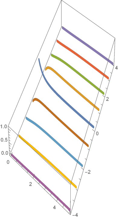
We plot this for integers −4≤n≤4-4\leq n\leq 4 in the range 0≤t≤50\leq t\leq 5 in the first graph in Figure 2, plotted using standard functions in Mathematica, and there it can be seen that there is a damped oscillatory behaviour.
Refer to caption
Refer to caption
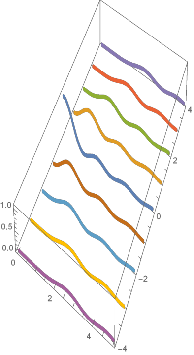
Figure 2: The time evolution of states on the integers for the exponential and diffusion respectively.

We should compare this geodesic calculation with the usual diffusion equation on ℤ\mathbb{Z} which also gives a time dependent state. Diffusion is defined in terms of a Lagrangian Δ\Delta and Lagrangians on graphs have been studied for some time (e.g., [7]). We use the special case for diffusion of a density f:ℤ×[0,∞)→ℝf\colon\mathbb{Z}\times[0,\infty)\rightarrow\mathbb{R} given by, for λ>0\lambda>0,

d​f​(n)d​t=−λ⁡(Δ​f)​(n)=−λ⁡(2​f​(n)−f⁡(n−1)−f⁡(n+1)).\displaystyle\frac{\mathrm{d}f(n)}{\mathrm{d}t}=-\lambda(\Delta f)(n)=-\lambda(2f(n)-f(n-1)-f(n+1)).

This is just (5.3) with f⁡(n)=αt​(δn)f(n)=\alpha_{t}(\delta_{n}) but with X+1=X−1=−λ<0X^{+1}=X^{-1}=-\lambda<0, i.e., with an “imaginary” vector field satisfying X−1=X+1¯X^{-1}=\overline{X^{+1}}. We start at t=0t=0 with f⁡(n)=0f(n)=0 for n≠0n\neq 0 and f⁡(0)=1f(0)=1, and this is just the same as the initial condition for αt\alpha_{t} previously. Now the Proposition 5.1 gives the solution for ff as a function of tt in the case λ=1\lambda=1 as

f=exp(tX∘ω)=(F10(;1;t2)z0+∑n>00F1(;n+1;t2)n!(tnzn+tnz−n))e−2​t∈ℂℤ.\displaystyle f=\exp(tX\circ\omega)=\bigg({}_{0}F_{1}\big(;1;t^{2}\big)z_{0}+\sum_{n>0}\dfrac{{}_{0}F_{1}\big(;n+1;t^{2}\big)}{n!}\big(t^{n}z_{n}+t^{n}z_{-n}\big)\bigg){\rm e}^{-2t}\in\mathbb{C}\mathbb{Z}.

We plot this for −4≤n≤4-4\leq n\leq 4 and 0≤t≤50\leq t\leq 5 as before in the second graph in Figure 2. For both the exponential and the diffusion we have one real parameter, |X+1|\big|X^{+1}\big| and λ\lambda respectively. We can see from the graphs that the behaviour of the states in the two cases is different, with the exponential giving “damped oscillations” and the diffusion giving a monotonic decrease at z0z_{0}.

6 The exponential map on quantum 𝑺​𝑼𝟐\bm{SU_{2}}

We use the matrix quantum group ℂq​[S​U2]\mathbb{C}_{q}[SU_{2}] as given by Woronowicz [24] and quantum enveloping algebra Uq​(𝔰​𝔲2)U_{q}({\mathfrak{su}}_{2}) as given in [14, 20]. There is a dual pairing between H=ℂq​[S​U2]H=\mathbb{C}_{q}[SU_{2}] and H′=Uq​(𝔰​𝔲2)H^{\prime}=U_{q}({\mathfrak{su}}_{2}). (We just say dual pairing as HH is infinite-dimensional and we need to be careful about duals.)

Definition 6.1.

For q∈ℂ∗q\in\mathbb{C}^{*} with q2≠−1q^{2}\neq-1, we define the quantum group ℂq​[S​U2]\mathbb{C}_{q}[SU_{2}] to have generators aa, bb, cc, dd with relations

ba=qab,ca=qac,db=qbd,dc=qcd,cb=bc,da−ad=q(1−q−2)bc,ad−q−1bc=1.\displaystyle\begin{split}&ba=qab,\qquad ca=qac,\qquad db=qbd,\qquad dc=qcd,\qquad cb=bc,\\ &da-ad=q\big(1-q^{-2}\big)bc,\qquad ad-q^{-1}bc=1.\end{split}

This is a Hopf algebra with coproduct, antipode and counit

Δ⁡(a)=a​⊗a+b​⊗c,Δ⁡(b)=b​⊗d+a​⊗b,Δ⁡(c)=c​⊗a+d​⊗c,\displaystyle\Delta(a)=a\mathop{\otimes}a+b\mathop{\otimes}c,\qquad\Delta(b)=b\mathop{\otimes}d+a\mathop{\otimes}b,\qquad\Delta(c)=c\mathop{\otimes}a+d\mathop{\otimes}c,
Δ⁡(d)=d​⊗d+c​⊗b,S⁡(a)=d,S⁡(b)=−q​b,S⁡(c)=−q−1​c,S⁡(d)=a,\displaystyle\Delta(d)=d\mathop{\otimes}d+c\mathop{\otimes}b,\qquad S(a)=d,\qquad S(b)=-qb,\qquad S(c)=-q^{-1}c,\qquad S(d)=a,
ϵ⁡(a)=ϵ⁡(d)=1,ϵ⁡(b)=ϵ⁡(c)=0.\displaystyle\epsilon(a)=\epsilon(d)=1,\qquad\epsilon(b)=\epsilon(c)=0.

This is a Hopf ∗*-algebra with a∗=da^{*}=d, d∗=ad^{*}=a, c∗=−q​bc^{*}=-qb and b∗=−q−1​cb^{*}=-q^{-1}c for qq real. We define a grade on monomials in generations by |a|=|c|=1|a|=|c|=1 and |b|=|d|=−1|b|=|d|=-1.

Definition 6.2.

Uq​(𝔰​𝔲2)U_{q}({\mathfrak{su}}_{2}) has generators X+X_{+}, X−X_{-}, q±H2q^{\pm\frac{H}{2}}, where we have relations

q−H2​qH2=qH2​q−H2=1,qH2​X±​q−H2=q±​X±,[X+,X−]=qH−q−Hq−q−1,\displaystyle q^{-\frac{H}{2}}q^{\frac{H}{2}}=q^{\frac{H}{2}}q^{-\frac{H}{2}}=1,\qquad q^{\frac{H}{2}}X_{\pm}q^{-\frac{H}{2}}=q^{\pm}X_{\pm},\qquad[X_{+},X_{-}]=\dfrac{q^{H}-q^{-H}}{q-q^{-1}},

and comultiplication, counit and antipode

Δ​q±H2=q±H2​⊗q±H2,Δ​X±=X±​⊗qH2+q−H2​⊗X±,\displaystyle\Delta q^{\pm\frac{H}{2}}=q^{\pm\frac{H}{2}}\mathop{\otimes}q^{\pm\frac{H}{2}},\qquad\Delta X_{\pm}=X_{\pm}\mathop{\otimes}q^{\frac{H}{2}}+q^{-\frac{H}{2}}\mathop{\otimes}X_{\pm},
ϵ⁡(q±H2)=1,ϵ⁡(X±)=0,S⁡(X±)=−q±​X±,S⁡(q±H2)=q∓H2.\displaystyle\epsilon\big(q^{\pm\frac{H}{2}}\big)=1,\qquad\epsilon(X_{\pm})=0,\qquad S(X_{\pm})=-q^{\pm}X_{\pm},\qquad S\big(q^{\pm\frac{H}{2}}\big)=q^{\mp\frac{H}{2}}.

As in Definition 2.1, these are dually paired by ⟨α,ti⟩j=ρ(α)i∈jℂ\langle\alpha,t^{i}{}_{j}\rangle=\rho(\alpha)^{i}{}_{j}\in\mathbb{C} where α∈Uq​(𝔰​𝔲2)\alpha\in U_{q}({\mathfrak{su}}_{2}) and t11=at^{1}{}_{1}=a, t12=bt^{1}{}_{2}=b, t21=ct^{2}{}_{1}=c and t22=dt^{2}{}_{2}=d and ρ:Uq​(𝔰​𝔲2)→M2​(ℂ)\rho\colon U_{q}({\mathfrak{su}}_{2})\rightarrow M_{2}(\mathbb{C}) is the representation (where r=qr=\sqrt{q})

ρ⁡(qH2)=(r001r),ρ⁡(X+)=(0100),ρ⁡(X−)=(0010).\displaystyle\rho(q^{\frac{H}{2}})=\left(\begin{matrix}r&0\\ 0&\frac{1}{r}\end{matrix}\right),\qquad\rho(X_{+})=\left(\begin{matrix}0&1\\ 0&0\end{matrix}\right),\qquad\rho(X_{-})=\left(\begin{matrix}0&0\\ 1&0\end{matrix}\right).
Definition 6.3 ([24]).

The left covariant 33D calculus for the quantum group ℂq​[S​U2]\mathbb{C}_{q}[SU_{2}] has generators e0e^{0} and e±e^{\pm}. The relations are

e±​a=q​a​e±,e±​b=q−1​b​e±,e±​c=q​c​e±,e±​d=q−1​d​e±,\displaystyle e^{\pm}a=qae^{\pm},\qquad e^{\pm}b=q^{-1}be^{\pm},\qquad e^{\pm}c=qce^{\pm},\qquad e^{\pm}d=q^{-1}de^{\pm},
e0​a=q2​a​e0,e0​b=q−2​b​e0,e0​c=q2​c​e0,e0​d=q−2​d​e0,\displaystyle e^{0}a=q^{2}ae^{0},\qquad e^{0}b=q^{-2}be^{0},\qquad e^{0}c=q^{2}ce^{0},\qquad e^{0}d=q^{-2}de^{0},

and exterior derivative and the ∗*-operator

d​a=a​e0+q​b​e+,d​b=a​e−−q−2​b​e0,d​c=c​e0+q​d​e+,d​d=c​e−−q−2​d​e0,\displaystyle\mathrm{d}a=ae^{0}+qbe^{+},\qquad\mathrm{d}b=ae^{-}-q^{-2}be^{0},\qquad\mathrm{d}c=ce^{0}+qde^{+},\qquad\mathrm{d}d=ce^{-}-q^{-2}de^{0},
e0∗=−e0,e+⁣∗=−q−1e−,e−⁣∗=−qe+.\displaystyle e^{0*}=-e^{0},\qquad e^{+*}=-q^{-1}e^{-},\qquad e^{-*}=-qe^{+}.

Now using ω:H→ΛH1\omega\colon H\rightarrow\Lambda_{H}^{1} from (3.4) we calculate

ω⁡(a)=q−2​e0,ω⁡(b)=q−1​e−,ω⁡(c)=q2​e+,ω⁡(d)=−e0.\displaystyle\omega(a)=q^{-2}e^{0},\qquad\omega(b)=q^{-1}e^{-},\qquad\omega(c)=q^{2}e^{+},\qquad\omega(d)=-e^{0}. (6.1)

We define e0e_{0}, e+e_{+}, e−e_{-} to be the dual basis of e0e^{0}, e+e^{+}, e−e^{-}, i.e., ⟨ei,ej⟩=δi​j\langle e_{i},e^{j}\rangle=\delta_{ij}. Now every ei∘ωe_{i}\circ\omega gives a map from ℂq​[S​U2]\mathbb{C}_{q}[SU_{2}] to ℂ\mathbb{C}. We shall identify ei∘ωe_{i}\circ\omega as an element of Uq​(𝔰​𝔲2)U_{q}({\mathfrak{su}}_{2}). The first step is to apply ei∘ωe_{i}\circ\omega to a product.

Lemma 6.4.

For all g,h∈ℂq​[S​U2]g,h\in\mathbb{C}_{q}[SU_{2}]

(e±∘ω)​(g​h)=(e±∘ω)​(g)​ϵ​(h)+q−|g|​ϵ​(g)​(e±∘ω)​(h),\displaystyle(e_{\pm}\circ\omega)(gh)=(e_{\pm}\circ\omega)(g)\epsilon(h)+q^{-|g|}\epsilon(g)(e_{\pm}\circ\omega)(h),
(e0∘ω)​(g​h)=(e0∘ω)​(g)​ϵ​(h)+q−2​|g|​ϵ​(g)​(e0∘ω)​(h).\displaystyle(e_{0}\circ\omega)(gh)=(e_{0}\circ\omega)(g)\epsilon(h)+q^{-2|g|}\epsilon(g)(e_{0}\circ\omega)(h).
Proof.

By definition

ω⁡(g​h)=d⁡(g(2)​h(2))​S−1​(g(1)​h(1))=ω⁡(g)​ϵ​(h)+g(2)​ω​(h)​S−1​(g(1)).\displaystyle\omega(gh)=\mathrm{d}\big(g_{(2)}h_{(2)}\big)S^{-1}\big(g_{(1)}h_{(1)}\big)=\omega(g)\epsilon(h)+g_{(2)}\omega(h)S^{-1}\big(g_{(1)}\big).

Now ej​g(2)​ei​S−1​(g(1))=0e_{j}g_{(2)}e^{i}S^{-1}\big(g_{(1)}\big)=0 unless i=ji=j, so we need to show

g(2)​e±​S−1​(g(1))=ϵ⁡(g)​q−|g|​e±,g(2)​e0​S−1​(g(1))=ϵ⁡(g)​q−2​|g|​e0.\displaystyle g_{(2)}e^{\pm}S^{-1}\big(g_{(1)}\big)=\epsilon(g)q^{-|g|}e^{\pm},\qquad g_{(2)}e^{0}S^{-1}\big(g_{(1)}\big)=\epsilon(g)q^{-2|g|}e^{0}.

It is enough to do this on the generators

a(2)​e±​S−1​(a(1))\displaystyle a_{(2)}e^{\pm}S^{-1}(a_{(1)}) =a​e±​S−1​(a)+c​e±​S−1​(b)\displaystyle=ae^{\pm}S^{-1}(a)+ce^{\pm}S^{-1}(b)
=a​e±​d−q−1​c​e±​b=q−1​(a​d−q−1​c​b)​e±=q−1​e±,\displaystyle=ae^{\pm}d-q^{-1}ce^{\pm}b=q^{-1}\big(ad-q^{-1}cb\big)e^{\pm}=q^{-1}e^{\pm},

and similarly for e0e^{0} and bb, cc, dd. ∎

We can use Lemma 6.4 to identify the coproduct of ei∘ωe_{i}\circ\omega, where the linear map g↦ϵ⁡(g)g\mapsto\epsilon(g) is just 1∈Uq​(𝔰​𝔲2)1\in U_{q}({\mathfrak{su}}_{2}). To do this we need to identify the map g↦qs​|g|​ϵ​(g)g\mapsto q^{s|g|}\epsilon(g).

Lemma 6.5.

For s∈ℝs\in\mathbb{R} and g∈ℂq​[S​U2]g\in\mathbb{C}_{q}[SU_{2}] we have ⟨qs​H,g⟩=qs​|g|​ϵ​(g)\langle q^{sH},g\rangle=q^{s|g|}\epsilon(g).

Proof.

As Δ​qs​H=qs​H​⊗qs​H\Delta q^{sH}=q^{sH}\mathop{\otimes}q^{sH} where ⟨qs​H,h​g⟩=⟨qs​H,h⟩​⟨qs​H,g⟩\big\langle q^{sH},hg\big\rangle=\big\langle q^{sH},h\big\rangle\big\langle q^{sH},g\big\rangle we only have to check the formula on the generators, and this is ⟨qs​H,ti⟩j=ρ(qs​H)ij\big\langle q^{sH},t^{i}{}_{j}\big\rangle=\rho\big(q^{sH}\big)^{i}{}_{j} using ρ⁡(qs​H)=(qs00q−s)\rho\big(q^{sH}\big)=\left(\begin{smallmatrix}q^{s}&0\\ 0&q^{-s}\end{smallmatrix}\right). ∎

Proposition 6.6.

In Uq​(𝔰​𝔲2)U_{q}({\mathfrak{su}}_{2}) we have (ei∘ω)​(h)=ev⁡(νi​⊗h)(e_{i}\circ\omega)(h)=\mathrm{ev}(\nu_{i}\mathop{\otimes}h) where νi∈Uq​(𝔰​𝔲2)\nu_{i}\in U_{q}({\mathfrak{su}}_{2}) is given by, where r=qr=\sqrt{q},

ν0=e0∘ω=1−q−2​Hq2−1,ν+=e+∘ω=r3​q−H2​X−,ν−=e−∘ω=r−1​q−H2​X+.\displaystyle\nu_{0}=e_{0}\circ\omega=\frac{1-q^{-2H}}{q^{2}-1},\qquad\nu_{+}=e_{+}\circ\omega=r^{3}q^{\frac{-H}{2}}X_{-},\qquad\nu_{-}=e_{-}\circ\omega=r^{-1}q^{\frac{-H}{2}}X_{+}.
Proof.

First we check that νi=ei∘ω\nu_{i}=e_{i}\circ\omega on the generators

ρ⁡(ν0)=(q−200−1),ρ⁡(ν+)=(00q20),ρ⁡(ν−)=(0q−100).\displaystyle\rho(\nu_{0})=\left(\begin{matrix}q^{-2}&0\\ 0&-1\end{matrix}\right),\qquad\rho(\nu_{+})=\left(\begin{matrix}0&0\\ q^{2}&0\end{matrix}\right),\qquad\rho(\nu_{-})=\left(\begin{matrix}0&q^{-1}\\ 0&0\end{matrix}\right).

Thus ν0\nu_{0} applied to bb, cc gives zero, and this is also true for e0∘ωe_{0}\circ\omega by (6.1). Also ν+\nu_{+} applied to aa, bb, dd gives zero, and this is also true for e+∘ωe_{+}\circ\omega by (6.1). Lastly ν−\nu_{-} applied to aa, cc, dd gives zero, and this is also true for e−∘ωe_{-}\circ\omega. We are left with the cases, for

(e0∘ω)​(a)=e0​(q−2​e0)=q−2=⟨ν0,a⟩,(e0∘ω)​(d)=e0​(−e0)=−1=⟨ν0,d⟩,\displaystyle(e_{0}\circ\omega)(a)=e_{0}\big(q^{-2}e^{0}\big)=q^{-2}=\langle\nu_{0},a\rangle,\qquad(e_{0}\circ\omega)(d)=e_{0}\big({-}e^{0}\big)=-1=\langle\nu_{0},d\rangle,
(e+∘ω)​(c)=q2=⟨ν+,c⟩,(e−∘ω)​(b)=q−1=⟨ν−,b⟩.\displaystyle(e_{+}\circ\omega)(c)=q^{2}=\langle\nu_{+},c\rangle,\qquad(e_{-}\circ\omega)(b)=q^{-1}=\langle\nu_{-},b\rangle. (6.2)

Now we need to show that we get equality on products of generators, which we show by induction. Suppose that is the dual ei∘ω=νie_{i}\circ\omega=\nu_{i} when applied to products of ≤n\leq n generators. If gg, hh are product of ≤n\leq n generators, then

ν±​(g​h)=ν±​(g)​ϵ​(h)+⟨q−H,g⟩​ν±​(h)=ν±​(g)​ϵ​(h)+q−|g|​ν±​(h),\displaystyle\nu_{\pm}(gh)=\nu_{\pm}(g)\epsilon(h)+\big\langle q^{-H},g\big\rangle\nu_{\pm}(h)=\nu_{\pm}(g)\epsilon(h)+q^{-|g|}\nu_{\pm}(h),

which is (e±∘ω)​(g​h)(e_{\pm}\circ\omega)(gh) by Lemma 6.4. Also from Lemma 6.5

ν0​(g​h)=1q2−1​ϵ​(g)​ϵ​(h)−1q2−1​⟨q−2​H,g​h⟩=ϵ⁡(g)​ϵ​(h)q2−1​(1−q−2​|g|​q−2​|h|),\displaystyle\nu_{0}(gh)=\dfrac{1}{q^{2}-1}\epsilon(g)\epsilon(h)-\dfrac{1}{q^{2}-1}\big\langle q^{-2H},gh\big\rangle=\dfrac{\epsilon(g)\epsilon(h)}{q^{2}-1}\big(1-q^{-2|g|}q^{-2|h|}\big),

whereas

(e0∘ω)​(g​h)\displaystyle(e_{0}\circ\omega)(gh) =ϵ⁡(h)q2−1​(ϵ⁡(g)−q−2​|g|​ϵ​(g))+q−2​|g|q2−1​(ϵ⁡(h)−q−2​|h|​ϵ​(h))​ϵ​(g)\displaystyle=\frac{\epsilon(h)}{q^{2}-1}\big(\epsilon(g)-q^{-2|g|}\epsilon(g)\big)+\frac{q^{-2|g|}}{q^{2}-1}\big(\epsilon(h)-q^{-2|h|}\epsilon(h)\big)\epsilon(g)
=ϵ⁡(g)​ϵ​(h)q2−1​(1−q−2​|g|​q−2​|h|)=ν0​(g​h)\displaystyle=\frac{\epsilon(g)\epsilon(h)}{q^{2}-1}\big(1-q^{-2|g|}q^{-2|h|}\big)=\nu_{0}(gh)

as required. ∎

The previously calculated exponentials in this case give a formal exponential of a linear combination of the ν\nu in Uq​(𝔰​𝔲2)U_{q}({\mathfrak{su}}_{2}). We consider that there is little reason to just write out such a formal sum. However, we can calculate the time evolution of certain states on ℂq​[S​U2]\mathbb{C}_{q}[SU_{2}]. We use states of the form ψt​(a)=ϕ⁡(m⁡(t)​a​m​(t)∗)\psi_{t}(a)=\phi(m(t)am(t)^{*}) where (m⁡(t))(m(t)) is defined in Theorem 3.4. First we look at the real vector field X=i​e0X={\rm i}e_{0}.

Proposition 6.7.

For any monomial yy in the generators aa, bb, cc, dd we have ν0​(y)=−[−|y|]q2​ϵ​(y)\nu_{0}(y)=-[-|y|]_{q^{2}}\epsilon(y) using the q2q^{2} integer [n]q2=(1−q2​n)/(1−q2)[n]_{q^{2}}=\big(1-q^{2n}\big)/\big(1-q^{2}\big), and

exp⁡(i​t​ν0)​(y)=exp⁡(−i​t​[−|y|]q2)​ϵ​(y).\exp({\rm i}t\nu_{0})(y)=\exp\big({-}{\rm i}t[-|y|]_{q^{2}}\big)\epsilon(y).
Proof.

The first result is given by using the definition of ν0\nu_{0} in Proposition 6.6 with Lemma 6.5. Then ν02​(y)=ν0​(y(1))​ν0​(y(2))=[−|y(1)|]q2​[−|y(2)|]q2​ϵ​(y(1))​ϵ​(y(2))\nu_{0}^{2}(y)=\nu_{0}(y_{(1)})\nu_{0}(y_{(2)})=[-|y_{(1)}|]_{q^{2}}[-|y_{(2)}|]_{q^{2}}\epsilon(y_{(1)})\epsilon(y_{(2)}). As ϵ\epsilon annihilates bb and cc we must have yy containing no bb, cc for this to be nonzero. As Δ​a=a​⊗a+b​⊗c\Delta a=a\mathop{\otimes}a+b\mathop{\otimes}c and Δ​d=d​⊗d+c​⊗b\Delta d=d\mathop{\otimes}d+c\mathop{\otimes}b we have ν02​(y)=ν0​(y)2\nu_{0}^{2}(y)=\nu_{0}(y)^{2}. This continues with higher powers. ∎

Proposition 6.8.

For the real vector field X=i​e0X={\rm i}e_{0} we have ((summing over monomials in 𝑂𝑃𝐸𝑁m⁡(0))m(0))

m⁡(t)=m⁡(0)​exp⁡(i​t​[−|m⁡(0)|]q2).m(t)=m(0)\exp\big({\rm i}t[-|m(0)|]_{q^{2}}\big).
Proof.

We have from Theorem 3.4 and Proposition 6.7

m(t)=m(0)(1)exp(−ite0∘ω)(m(0)(2))=m(0)(1)exp(it[−|m(0)(2)|]q2)ϵ(m(0)(2)).m(t)=m(0)_{(1)}\exp(-{\rm i}te_{0}\circ\omega)\big(m(0)_{(2)}\big)=m(0)_{(1)}\exp\big({\rm i}t[-|m(0)_{(2)}|]_{q^{2}}\big)\epsilon\big(m(0)_{(2)}\big).

Note that for a monomial m⁡(0)m(0), we have |m​(0)(2)|=|m⁡(0)||m(0)_{(2)}|=|m(0)| giving the answer. ∎

We now look at the X=γ​e++δ​e−X=\gamma e_{+}+\delta e_{-} case. In the previous examples we had ψ0​(a)=ϕ⁡(m⁡(0)​a​m​(0)∗)=ϵ⁡(a)\psi_{0}(a)=\phi(m(0)am(0)^{*})\allowbreak=\epsilon(a). However, because of the complexity of the calculation we will simply calculate m⁡(t)m(t) for m⁡(0)m(0) a generator.

Proposition 6.9.

For X=γ​e++δ​e−X=\gamma e_{+}+\delta e_{-} we calculate m⁡(t)m(t) for m⁡(0)m(0) being generator to be

m⁡(0)=a,m⁡(t)=a​cosh⁡(t​q​γ​δ)−b​q2​γq​γ​δ​sinh⁡(t​q​γ​δ),\displaystyle m(0)=a,\qquad m(t)=a\cosh\big(t\sqrt{q\gamma\delta}\big)-b\frac{q^{2}\gamma}{\sqrt{q\gamma\delta}}\sinh\big(t\sqrt{q\gamma\delta}\big),
m⁡(0)=b,m⁡(t)=b​cosh⁡(t​q​γ​δ)−a​q−1​δq​γ​δ​sinh⁡(t​q​γ​δ),\displaystyle m(0)=b,\qquad m(t)=b\cosh\big(t\sqrt{q\gamma\delta}\big)-a\frac{q^{-1}\delta}{\sqrt{q\gamma\delta}}\sinh\big(t\sqrt{q\gamma\delta}\big),
m⁡(0)=c,m⁡(t)=c​cosh⁡(t​q​γ​δ)−d​q2​γq​γ​δ​sinh⁡(t​q​γ​δ),\displaystyle m(0)=c,\qquad m(t)=c\cosh\big(t\sqrt{q\gamma\delta}\big)-d\frac{q^{2}\gamma}{\sqrt{q\gamma\delta}}\sinh\big(t\sqrt{q\gamma\delta}\big),
m⁡(0)=d,m⁡(t)=d​cosh⁡(t​q​γ​δ)−c​q−1​δq​γ​δ​sinh⁡(t​q​γ​δ).\displaystyle m(0)=d,\qquad m(t)=d\cosh\big(t\sqrt{q\gamma\delta}\big)-c\frac{q^{-1}\delta}{\sqrt{q\gamma\delta}}\sinh\big(t\sqrt{q\gamma\delta}\big).
Proof.

We get the corresponding element of the dual x=X∘ω=γ​ν++δ​ν−x=X\circ\omega=\gamma\nu_{+}+\delta\nu_{-}. Then xn​(h)=x⁡(h(1))​xn−1​(h(2))x^{n}(h)=x\big(h_{(1)}\big)x^{n-1}\big(h_{(2)}\big), so from (6.2)

xn​(a)=q−1​δ​xn−1​(c),xn​(b)=q−1​δ​xn−1​(d),\displaystyle x^{n}(a)=q^{-1}\delta x^{n-1}(c),\qquad x^{n}(b)=q^{-1}\delta x^{n-1}(d),
xn​(c)=q2​γ​xn−1​(a),xn​(d)=q2​γ​xn−1​(b).\displaystyle x^{n}(c)=q^{2}\gamma x^{n-1}(a),\qquad x^{n}(d)=q^{2}\gamma x^{n-1}(b).

These give

xodd​(a)=xodd​(d)=0,xeven​(b)=xeven​(c)=0,\displaystyle x^{\text{odd}}(a)=x^{\text{odd}}(d)=0,\qquad x^{\text{even}}(b)=x^{\text{even}}(c)=0,
x2​n​(a)=(q​γ​δ)n=x2​n​(d),x2​n+1​(b)=qn−1​γn​δn+1,x2​n+1​(c)=qn+2​γn+1​δn,\displaystyle x^{2n}(a)=(q\gamma\delta)^{n}=x^{2n}(d),\qquad x^{2n+1}(b)=q^{n-1}\gamma^{n}\delta^{n+1},\qquad x^{2n+1}(c)=q^{n+2}\gamma^{n+1}\delta^{n},

so for the formal exponential e−t​x​(h)=∑n≥0(−t​x)nn!​(h){\rm e}^{-tx}(h)=\sum_{n\geq 0}\dfrac{(-tx)^{n}}{n!}(h)

e−t​x​(a)=∑n≥0t2​n​(−x)2​n2​n!​(a)=∑n≥=0t2​n​(q​γ​δ)n2​n!=cosh⁡(t​q​γ​δ)=e−t​x​(d),\displaystyle{\rm e}^{-tx}(a)=\sum_{n\geq 0}\dfrac{t^{2n}(-x)^{2n}}{2n!}(a)=\sum_{n\geq=0}\dfrac{t^{2n}(q\gamma\delta)^{n}}{2n!}=\cosh\big(t\sqrt{q\gamma\delta}\big)={\rm e}^{-tx}(d),
e−t​x(b)=∑n≥0t2​n+1​(−x)2​n+1(2​n+1)!(b)=−∑n≥0t2​n+1​qn−1​γn+1​δn(2​n+1)!=−q−1​δq​γ​δsinh(tq​γ​δ),\displaystyle{\rm e}^{-tx}(b)=\sum_{n\geq 0}\dfrac{t^{2n+1}(-x)^{2n+1}}{(2n+1)!}(b)=-\sum_{n\geq 0}\dfrac{t^{2n+1}q^{n-1}\gamma^{n+1}\delta^{n}}{(2n+1)!}=\frac{-q^{-1}\delta}{\sqrt{q\gamma\delta}}\sinh\big(t\sqrt{q\gamma\delta}\big),
e−t​x(c)=∑n≥0t2​n+1​(−x)2​n+1(2​n+1)!(c)=−∑n≥0t2​n+1​qn+2​γn+1​δn(2​n+1)!=−q2​γq​γ​δsinh(tq​γ​δ),\displaystyle{\rm e}^{-tx}(c)=\sum_{n\geq 0}\dfrac{t^{2n+1}(-x)^{2n+1}}{(2n+1)!}(c)=-\sum_{n\geq 0}\dfrac{t^{2n+1}q^{n+2}\gamma^{n+1}\delta^{n}}{(2n+1)!}=\frac{-q^{2}\gamma}{\sqrt{q\gamma\delta}}\sinh\big(t\sqrt{q\gamma\delta}\big),

and we use Theorem 3.4 to get the answer. ∎

Example 6.10.

For X=γ​e++δ​e−X=\gamma e_{+}+\delta e_{-} to be real by Proposition 3.3 we have γ∗=−q−1​δ\gamma^{*}=-q^{-1}\delta, so q​γ​δ=−q2​|γ|2=±i​q​|γ|\sqrt{q\gamma\delta}=\sqrt{-q^{2}|\gamma|^{2}}=\pm{\rm i}q|\gamma|. Then a special case of Proposition 6.9 gives

m⁡(0)=a,m⁡(t)=a​cosh⁡(i​q​|γ|​t)−b​q2​γi​q​|γ|​sinh⁡(i​q​|γ|​t)=a​cos⁡(q​|γ|​t)−b​q​γ|γ|​sin⁡(q​|γ|​t).\displaystyle m(0)=a,\qquad m(t)=a\cosh({\rm i}q|\gamma|t)-b\frac{q^{2}\gamma}{iq|\gamma|}\sinh({\rm i}q|\gamma|t)=a\cos(q|\gamma|t)-b\frac{q\gamma}{|\gamma|}\sin(q|\gamma|t).

Using an exponential map on an initial state will give a time evolution preserving the normalisation as long as we use a real invariant vector field. We now check this in our case of γ​e++δ​e−\gamma e_{+}+\delta e_{-}. We begin with the Haar integral on ℂq​[S​U2]\mathbb{C}_{q}[SU_{2}] which is zero on all basis elements an​br​csa^{n}b^{r}c^{s} and dn​br​csd^{n}b^{r}c^{s} except

ϕ⁡((b​c)r)=(−1)r​qr[r+1]q2.\displaystyle\phi((bc)^{r})=\frac{(-1)^{r}q^{r}}{[r+1]_{q^{2}}}.

Starting from m⁡(0)=am(0)=a we find from ϕ⁡(m⁡(t)​m​(t)∗)\phi(m(t)m(t)^{*}) that ψt​(1)=q21+q2\psi_{t}(1)=\frac{q^{2}}{1+q^{2}} which is independent of tt as required.

7 Sweedler–Taft algebra

We will now look at the Sweedler–Taft algebra HH of dimension 44. This Hopf algebra does not have a normalised Haar integral, and since we use the integral in finding the “state” we shall get an algebraic construction which is nothing like the C∗C^{*}-algebra framework. The Sweedler–Taft algebra [21] is a unital algebra with generators xx, tt and relations

t2=1,x2=0,x​t=−t​x,\displaystyle t^{2}=1,\qquad x^{2}=0,\qquad xt=-tx,

so it is 4-dimensional with basis {1,t,x,x​t}\{1,t,x,xt\}. The following operations make it into a Hopf algebra

Δ​1=1​⊗1,Δ​t=t​⊗t,Δ​x=x​⊗t+1​⊗x,Δ⁡(t​x)=t​x​⊗1+t​⊗t​x,\displaystyle\Delta 1=1\mathop{\otimes}1,\qquad\Delta t=t\mathop{\otimes}t,\qquad\Delta x=x\mathop{\otimes}t+1\mathop{\otimes}x,\qquad\Delta(tx)=tx\mathop{\otimes}1+t\mathop{\otimes}tx,
ϵ⁡(t)=ϵ⁡(1)=1,ϵ⁡(x)=ϵ⁡(t​x)=0,S​t=t,S​x=t​x.\displaystyle\epsilon(t)=\epsilon(1)=1,\qquad\epsilon(x)=\epsilon(tx)=0,\qquad St=t,\qquad Sx=tx.

We make the Sweedler–Taft algebra into a Hopf ∗*-algebra by t∗=tt^{*}=t and x∗=xx^{*}=x.

There is a unique 2D bicovariant calculus with right ideal ℐ⊂H+=ker⁡ϵ\mathcal{I}\subset H^{+}=\ker\epsilon generated by x−x​tx-xt and the ∗* operation above has S⁡((x−x​t)∗)=x−x​tS((x-xt)^{*})=x-xt and so gives a ∗*-calculus [5]. We take the basis e1=[x]∈H+/ℐ=Λ1e^{1}=[x]\in H^{+}/\mathcal{I}=\Lambda^{1} and e2=[t−1]e^{2}=[t-1] of Λ1\Lambda^{1} and relations

dt=te2,dx=xe2+e1,d(xt)=te1,e2t=−te2,e1t=te1,e1x=xe1,e2x=−xe2−2e1,e1∧e1=e2∧e2=0,e1∧e2=e2∧e1,de2=0,de1=−e1∧e2.\displaystyle\begin{split}&\mathrm{d}t=te^{2},\qquad\mathrm{d}x=xe^{2}+e^{1},\qquad\mathrm{d}(xt)=te^{1},\\ &e^{2}t=-te^{2},\qquad e^{1}t=te^{1},\qquad e^{1}x=xe^{1},\qquad e^{2}x=-xe^{2}-2e^{1},\\ &e^{1}\wedge e^{1}=e^{2}\wedge e^{2}=0,\qquad e^{1}\wedge e^{2}=e^{2}\wedge e^{1},\qquad\mathrm{d}e^{2}=0,\qquad\mathrm{d}e^{1}=-e^{1}\wedge e^{2}.\end{split}

Then d​t∗=−e2​t\mathrm{d}t^{*}=-e^{2}t gives e2∗=−e2e^{2}{}^{*}=-e^{2} and d​x∗=x​e2+e1\mathrm{d}x^{*}=xe^{2}+e^{1} gives e1∗=−e1e^{1}{}^{*}=-e^{1}. We introduce a basis of left invariant right vector fields e1e_{1} and e2e_{2} dual to e1,e2∈Λ1e^{1},e^{2}\in\Lambda^{1}. From (3.4) we find ω⁡(t)=−e2\omega(t)=-e^{2}, ω⁡(x)=−e1\omega(x)=-e^{1} and ω⁡(t​x)=−e1\omega(tx)=-e^{1}. Now we find ei∘ω∈H′e_{i}\circ\omega\in H^{\prime}. We get ei∘ω⁡(1)=0e_{i}\circ\omega(1)=0 and

e2∘ω⁡(t)=−1,e2∘ω⁡(x)=e2∘ω⁡(t​x)=0,e1∘ω⁡(t)=0,\displaystyle e_{2}\circ\omega(t)=-1,\qquad e_{2}\circ\omega(x)=e_{2}\circ\omega(tx)=0,\qquad e_{1}\circ\omega(t)=0,
e1∘ω⁡(x)=e1∘ω⁡(t​x)=−1.\displaystyle e_{1}\circ\omega(x)=e_{1}\circ\omega(tx)=-1.

The dual basis elements corresponding to 11, tt, xx, t​xtx are δ1\delta_{1}, δt\delta_{t}, δx\delta_{x}, δt​x\delta_{tx} and their products are

δ1.δ1=δ1,δt.δt=δt,δx.δt=δx=δ1.δx,δt​x.δ1=δt​x=δt.δt​x,\displaystyle\delta_{1}.\delta_{1}=\delta_{1},\qquad\delta_{t}.\delta_{t}=\delta_{t},\qquad\delta_{x}.\delta_{t}=\delta_{x}=\delta_{1}.\delta_{x},\qquad\delta_{tx}.\delta_{1}=\delta_{tx}=\delta_{t}.\delta_{tx},

and any other product is zero. Then e1∘ω=−δte_{1}\circ\omega=-\delta_{t} and e2∘ω=−δx−δt​xe_{2}\circ\omega=-\delta_{x}-\delta_{tx}. The vector field X=a​e1+b​e2X=ae_{1}+be_{2} for a,b∈ℂa,b\in\mathbb{C} has

X∘ω=−a​δt−b⁡(δx+δt​x),\displaystyle X\circ\omega=-a\delta_{t}-b(\delta_{x}+\delta_{tx}),
(X∘ω)2=a2​δt2+b2​(δx+δt​x)2+a​b​δt​(δx+δt​x)+a​b​(δx+δt​x)​δt=−a⁡(X∘ω),\displaystyle(X\circ\omega)^{2}=a^{2}\delta^{2}_{t}+b^{2}(\delta_{x}+\delta_{tx})^{2}+ab\delta_{t}(\delta_{x}+\delta_{tx})+ab(\delta_{x}+\delta_{tx})\delta_{t}=-a(X\circ\omega),

so adding a time parameter ss as usual (tt being used already)

exp⁡(−s⁡(X∘ω))\displaystyle\exp(-s(X\circ\omega)) =ϵ−s⁡(X∘ω)+(−s⁡(X∘ω))22!+(−s⁡(X∘ω))33!+⋯\displaystyle=\epsilon-s(X\circ\omega)+\frac{(-s(X\circ\omega))^{2}}{2!}+\frac{(-s(X\circ\omega))^{3}}{3!}+\cdots
=ϵ−ea​s−1a​(X∘ω),\displaystyle=\epsilon-\dfrac{{\rm e}^{as}-1}{a}(X\circ\omega),

so from Theorem 3.4

m⁡(s)=m⁡(0)+m​(0)(1)​1−es​aa​(X∘ω)​(m​(0)(2)).\displaystyle m(s)=m(0)+m(0)_{(1)}\dfrac{1-{\rm e}^{sa}}{a}(X\circ\omega)(m(0)_{(2)}). (7.1)

We now turn to the inner product and definition of real vector fields. The Haar integral [5] is given by ϕ⁡(t​x)=λ\phi(tx)=\lambda where λ\lambda is arbitrary and ϕ\phi of all other basis elements, including 11, to be zero. For Proposition 3.2 we require ϕ~\phi to be Hermitian, so λ\lambda is imaginary. Applying this ϕ\phi in the formula for the inner product gives all left invariant vector fields being real, as ϕ⁡(1)=0\phi(1)=0. Note that this definition of reality corresponds to preserving the inner product in Proposition 3.1, rather than what in this case is the stronger condition on duals in Proposition 3.3.

Example 7.1.

Set m⁡(0)=t+xm(0)=t+x and X=a​e1+b​e2X=ae_{1}+be_{2} as above. Then by (7.1)

m⁡(s)\displaystyle m(s) =t+x+1−es​aa​(t⁡(X∘ω)​(t)+1​(X∘ω⁡(x))+x⁡(X∘ω)​(t))\displaystyle=t+x+\dfrac{1-{\rm e}^{sa}}{a}(t(X\circ\omega)(t)+1(X\circ\omega(x))+x(X\circ\omega)(t))
=t+x+1−es​aa​(−t​b−x​b−a).\displaystyle=t+x+\dfrac{1-{\rm e}^{sa}}{a}(-tb-xb-a).

To calculate the value of the “state” ψs\psi_{s} in ϕ⁡(m⁡(t)​a​m​(t)∗)\phi(m(t)am(t)^{*}) we set m⁡(s)=m1​1+mt​t+mx​x+mt​x​t​xm(s)=m_{1}1+m_{t}t+m_{x}x+m_{tx}tx for mi∈ℂm_{i}\in\mathbb{C} then for the Haar measure ϕ\phi the map a↦ϕ⁡(m​a​m∗)a\mapsto\phi(mam^{*}) is the element of the dual

λ​δ1​(−m1​mt​x¯+mt​mx¯−mx​mt¯+mt​x​m1¯)+λ​δt​(m1​mx¯−mt​mt​x¯−mx​m1¯+mt​x​mt¯)\displaystyle\lambda\delta_{1}(-m_{1}\overline{m_{tx}}+m_{t}\overline{m_{x}}-m_{x}\overline{m_{t}}+m_{tx}\overline{m_{1}})+\lambda\delta_{t}(m_{1}\overline{m_{x}}-m_{t}\overline{m_{tx}}-m_{x}\overline{m_{1}}+m_{tx}\overline{m_{t}})
+λ​δx​(−m1​mt¯+mt​m1¯)+λ​δt​x​(|m1|2−|mt|2).\displaystyle\qquad{}+\lambda\delta_{x}(-m_{1}\overline{m_{t}}+m_{t}\overline{m_{1}})+\lambda\delta_{tx}\big(|m_{1}|^{2}-|m_{t}|^{2}\big).

Substituting the values for m⁡(s)m(s) gives

ψs=λ⁡(δt−δx)​(es​a−es​a¯+|es​a−1|2​(b¯a¯−ba))\displaystyle\psi_{s}=\lambda(\delta_{t}-\delta_{x})\left({\rm e}^{sa}-{\rm e}^{s\overline{a}}+\big|{\rm e}^{sa}-1\big|^{2}\left(\frac{\overline{b}}{\overline{a}}-\frac{b}{a}\right)\right)
ψ_s =+λ​δt​x​(|es​a−1|2​(1−|ba|2)−1−ba​(es​a−1)−b¯a¯​(es​a¯−1)).\displaystyle\hphantom{\psi_s =}{}+\lambda\delta_{tx}\left(\big|{\rm e}^{sa}-1\big|^{2}\left(1-\left|\frac{b}{a}\right|^{2}\right)-1-\dfrac{b}{a}\big({\rm e}^{sa}-1\big)-\frac{\overline{b}}{\overline{a}}\big({\rm e}^{s\overline{a}}-1\big)\right).

Acknowledgements

We would like to thank the editor and referees for many useful comments. Computer algebra and graphs were done on Mathematica.

References

  • [1] Beggs E.J., Differential and holomorphic differential operators on noncommutative algebras, Russ. J. Math. Phys. 22 (2015), 279–300, arXiv:1209.3900.
  • [2] Beggs E.J., Noncommutative geodesics and the KSGNS construction, J. Geom. Phys. 158 (2020), 103851, 14 pages, arXiv:1811.07601.
  • [3] Beggs E.J., Majid S., Bar categories and star operations, Algebr. Represent. Theory 12 (2009), 103–152, arXiv:math.QA/0701008.
  • [4] Beggs E.J., Majid S., Quantum geodesics in quantum mechanics, arXiv:1912.13376.
  • [5] Beggs E.J., Majid S., Quantum Riemannian geometry, Grundlehren der mathematischen Wissenschaften, Vol. 355, Springer, Cham, 2020.
  • [6] Bresser K., Müller-Hoissen F., Dimakis A., Sitarz A., Non-commutative geometry of finite groups, J. Phys. A: Math. Gen. 29 (1996), 2705–2735.
  • [7] Chung F.R.K., Spectral graph theory, CBMS Regional Conference Series in Mathematics, Vol. 92, Amer. Math. Soc., Providence, RI, 1997.
  • [8] Dubois-Violette M., Masson T., On the first-order operators in bimodules, Lett. Math. Phys. 37 (1996), 467–474, arXiv:q-alg/9507028.
  • [9] Dubois-Violette M., Michor P.W., Connections on central bimodules in noncommutative differential geometry, J. Geom. Phys. 20 (1996), 218–232, arXiv:q-alg/9503020.
  • [10] Fiore G., Madore J., Leibniz rules and reality conditions, Eur. Phys. J. C Part. Fields 17 (2000), 359–366, arXiv:math.QA/9806071.
  • [11] Franz U., Lévy processes on quantum groups, in Probability on Algebraic Structures (Gainesville, FL, 1999), Contemp. Math., Vol. 261, Amer. Math. Soc., Providence, RI, 2000, 161–179.
  • [12] Gomez X., Majid S., Braided Lie algebras and bicovariant differential calculi over co-quasitriangular Hopf algebras, J. Algebra 261 (2003), 334–388, arXiv:math.QA/0112299.
  • [13] Hausner M., Schwartz J.T., Lie groups; Lie algebras, Gordon and Breach Science Publishers, New York – London – Paris, 1968.
  • [14] Kulish P.P., Reshetikhin N.Yu., Quantum linear problem for the sine-Gordon equation and higher representations, J. Sov. Math. 23 (1983), 2435–2441.
  • [15] Lance E.C., Hilbert C∗C^{*}-modules. A toolkit for operator algebraists, London Mathematical Society Lecture Note Series, Vol. 210, Cambridge University Press, Cambridge, 1995.
  • [16] Madore J., An introduction to noncommutative differential geometry and its physical applications, 2nd ed., London Mathematical Society Lecture Note Series, Vol. 257, Cambridge University Press, Cambridge, 1999.
  • [17] Majid S., Quantum and braided-Lie algebras, J. Geom. Phys. 13 (1994), 307–356, arXiv:hep-th/9303148.
  • [18] Majid S., Foundations of quantum group theory, Cambridge University Press, Cambridge, 1995.
  • [19] Mourad J., Linear connections in non-commutative geometry, Classical Quantum Gravity 12 (1995), 965–974.
  • [20] Sklyanin E.K., Some algebraic structures connected with the Yang–Baxter equation, Funct. Anal. Appl. 16 (1982), 263–270.
  • [21] Taft E.J., The order of the antipode of finite-dimensional Hopf algebra, Proc. Nat. Acad. Sci. USA 68 (1971), 2631–2633.
  • [22] Weisstein E.W., Generalized hypergeometric function, From MathWorld – A Wolfram Web Resource, https://mathworld.wolfram.com/GeneralizedHypergeometricFunction.html.
  • [23] Woronowicz S.L., Twisted SU⁡(2){\rm SU}(2) group. An example of a noncommutative differential calculus, Publ. Res. Inst. Math. Sci. 23 (1987), 117–181.
  • [24] Woronowicz S.L., Differential calculus on compact matrix pseudogroups (quantum groups), Comm. Math. Phys. 122 (1989), 125–170.