An Energy Sharing Mechanism Considering Network Constraints and Market Power Limitation

DER

Distributed energy resource.

GNE

Generalized Nash equilibrium.

GNG

Generalized Nash game.

LMP

Locational marginal price.

P2P

Peer-to-peer.

PV

Photovoltaic.

PoA

Price of anarchy.

$i,\mathcal{I}$

Index and set of prosumers.

$l,\mathcal{L}$

Index and set of lines.

$S_{i}$

Action set of prosumer $i$, and $S=\prod_{i\in\mathcal{I}}S_{i}$.

$J_{i}(p_{i})$

Cost or disutility function of prosumer $i$, and $J(p)=\sum_{i\in\mathcal{I}}J_{i}(p_{i})$.

$\Gamma_{i}(p,b)$

Total cost of prosumer $i$ with energy sharing, which equals $J_{i}(p_{i})+\lambda_{i}(-a\lambda_{i}+b_{i})$.

$u_{i}(b,p_{i})$

Payment to the market under the improved energy sharing mechanism.

$I$

Number of prosumers.

$p_{i}^{0}$

Original energy production of prosumer $i$.

$E_{i}^{0}$

Energy purchased from the main grid or aggregator of prosumer $i$.

$D_{i}^{0}$

Fixed demand of prosumer $i$.

$D_{i}$

Energy reduction of prosumer $i$.

$c_{i},d_{i}$

Coefficients of function $J_{i}(p_{i})$ for prosumer $i$.

$a$

Energy sharing market sensitivity.

$\hat{F}_{l}$

Power flow limit for line $l$; $\tilde{F}_{l}:=\hat{F}_{l}+\sum_{i=1}^{I}\pi_{il}(E_{i}^{0}-D_{i})$ and $F_{l}:=\hat{F}_{l}-\sum_{i=1}^{I}\pi_{il}(E_{i}^{0}-D_{i})$.

$\pi_{il}$

Line flow distribution factor from bus $i$ to line $l$.

$p_{i}$

Production adjustment of prosumer $i$.

$\lambda_{i}$

Energy sharing price for prosumer $i$.

$\lambda_{i}^{r}$

Regulated energy sharing price for prosumer $i$.

$q_{i}$

Amount of energy prosumer $i$ gets from sharing.

$b_{i}$

Bid of prosumer $i$ in the energy sharing market.

$\eta,\alpha_{l}^{\pm}$

Dual variables of problem (5).

$\beta_{i}$

Dual variables of problem (7).

$\kappa,\tau_{l}^{\pm}$

Dual variables of problem (10).

A set of networked prosumers indexed by $i\in\mathcal{I}=\{1,2,...,I\}$ is considered. For simplicity, we assume that each prosumer has a distributed generator (DG). The self-energy-balance condition for each prosumer $i\in\mathcal{I}$ is (1), where $p_{i}^{0}$ is prosumer $i$’s energy production, $E_{i}^{0}$ is its energy purchased from the main grid or aggregator, and $D_{i}^{0}$ is its demand.

All the prosumers take part in the interruptible/curtailable program that belongs to the incentive-based demand response [38]. In this type of demand response program, the participant is asked to adjust its demand to a predefined value and will receive payment or penalty based on its performance. Suppose prosumer $i\in\mathcal{I}$ is required to reduce its energy purchased from the main grid by $D_{i}$. To meet this requirement, prosumer $i\in\mathcal{I}$ increases its net production (which may be realized by increasing generation or reducing demand) by $p_{i}$, which becomes $(p_{i}^{0}-D_{i}^{0})+p_{i}$. This adjustment results in an extra cost or disutility $J_{i}(p_{i}):=c_{i}p_{i}^{2}+d_{i}p_{i}$ with constant coefficients $c_{i}>0$ and $d_{i}$.

Define self-sufficiency as the default response that every prosumer $i\in\mathcal{I}$ can only increase its net production to fulfill its desired energy purchase reduction, without trading energy with other prosumers: $(p_{i}^{0}-D_{i}^{0}+p_{i})+(E_{i}^{0}-D_{i})=0$, i.e., $p_{i}=D_{i}$ for all $i\in\mathcal{I}$. This self-sufficiency scheme is how the current system operates and is simple since no coordination among the prosumers is needed. But is there a more efficient way? In fact, energy sharing can provide a better solution to this problem. By allowing a prosumer with lower marginal disutility to produce more and sell energy to another prosumer with higher marginal disutility, a win-win situation can be reached among them.

Here, we use “sharing” not to refer to the natural pooling effect of the grid according to the Kirchhoff’s laws, but to the sharing of the prosumers’ adjustable capabilities. The questions we ask are: how to design a sharing market (coordination mechanism) to allow the prosumers jointly reduce their aggregate grid purchase by $\sum_{i}D_{i}$, as requested by the system operator, in a way that satisfies power balance and line limits? What are the optimality and convergence properties of a market equilibrium? By sharing their adjustable capabilities, an individual prosumer $i$ may not reduce its grid purchase by its scheduled amount $D_{i}$, some reduce more and some less, so that collectively, they provide the required total reduction $\sum_{i}D_{i}$. We hope that everyone is better off than without the sharing market, and the system approaches social optimality as the number of prosumers grows.

The remaining problem is how to design such a proper energy sharing mechanism, which is: 1) Private. Prosumer information privacy is preserved. 2) Motivated. Each prosumer has the incentive to participate in energy sharing. 3) Effective. Balance of supply and demand is reached, and physical network constraints are satisfied. 4) Flexible. Each prosumer has the freedom to choose between being a seller or a buyer.

In this paper, we propose an energy sharing mechanism considering network constraints. Denote the amount of energy prosumer $i\in\mathcal{I}$ purchases from the energy sharing market as $q_{i}$, so that it can meet the energy reduction requirement as $p_{i}+q_{i}=D_{i}$. A generalized demand function [39] is used to represent the relationship between $q_{i}$, prosumer bid $b_{i}$, and the energy sharing price $\lambda_{i}$. A different energy sharing price $\lambda_{i}$ is assigned to each prosumer $i\in\mathcal{I}$ to reflect its influence on power flow across transmission lines. To be specific:

1) The energy sharing amount of prosumer $i\in\mathcal{I}$ is:

where $q_{i}>0$ if prosumer $i$ is a buyer and $q_{i}<0$ if it is a seller; $a>0$ is the market sensitivity, which measures impact of prosumer bids on the energy sharing price; $b_{i}$ is the bid of prosumer $i$, showing its willingness to buy. Here, a linear function is used because it well captures the nature of the decrease in purchase/selling quantity with higher/lower prices and facilitates analysis. A linear function was also used in references [25, 26]. Note that the demand function can be represented as $q_{D}=-a_{D}\lambda+b_{D}$ with $a_{D}>0$. The supply function can be represented as $q_{S}=a_{S}\lambda-b_{S}$ with $a_{S}>0$, which is equivalent to $-q_{S}=-a_{S}\lambda+b_{S}$. For a prosumer, its sensitivity on buying or selling energy should be similar, i.e., $a_{D}\approx a_{S}$. Therefore, the demand and supply functions can be consolidated as a uniform form $q_{i}=-a\lambda_{i}+b_{i}$ with $a>0$.

2) Energy balancing condition:

It means the amount of energy sold to the energy sharing market equals the amount of energy bought from the market.

3) Power flow limits for the underlying network:

The nodal net power injection at node $i$ after sharing energy is $E_{i}^{0}-D_{i}+q_{i}$. Let $\hat{F}_{l},\forall l$ be the line capacity, then the network constraints are $-\hat{F}_{l}\leq\sum_{i=1}^{I}\pi_{il}(E_{i}^{0}-D_{i}+q_{i})\leq\hat{F}_{l},\forall l\in\mathcal{L}$, which is equivalent to (4) with $\tilde{F}_{l}:=\hat{F}_{l}+\sum_{i=1}^{I}\pi_{il}(E_{i}^{0}-D_{i})$ and $F_{l}:=\hat{F}_{l}-\sum_{i=1}^{I}\pi_{il}(E_{i}^{0}-D_{i})$. Direct current (DC) model is used to calculate the power flow on each line $l\in\mathcal{L}=\{1,...,L\}$. $\pi_{il}$ is the line flow distribution factor from prosumer $i$ to line $l$.

Remark on line flow distribution factor calculation. Consider the network as a directed graph with arbitrarily assigned directions. Let $C\in\{0,1,-1\}^{I\times L}$ be the incidence matrix of the network; $B\in(\mathbb{R}^{+})^{L\times L}$ be the diagonal matrix with diagonal terms being positive line weights derived from the standard DC power flow model, i.e., for a line $ij\in\mathcal{L}$, its weight $B_{ij}=|V_{i}||V_{j}|/x_{ij}$ where $|V_{i}|$ and $|V_{j}|$ are voltage magnitudes at nodes (prosumers) $i$ and $j$, respectively, and $x_{ij}$ is the reactance of inductive line $ij$. Let $\tilde{C}$ be a reduced incidence matrix by removing an arbitrary row of $C$ (without loss of generality, we remove the last row). Then the line flow distribution factor matrix $\Pi$ can be constructed as follows: first calculate $\tilde{\Pi}=-\left(\tilde{C}B\tilde{C}^{T}\right)^{-1}\tilde{C}B\in\mathbb{R}^{(I-1)\times L}$; then add an all-zero row of dimension $L$ to the bottom of $\tilde{\Pi}$ to obtain $\Pi$, whose element in $i$-th row, $l$-th column is $\pi_{il}$.

With all prosumers’ bids $b_{i},\forall i\in\mathcal{I}$, a central platform clears the market to determine the energy sharing quantities $q_{i},\forall i\in\mathcal{I}$ and prices $\lambda_{i},\forall i\in\mathcal{I}$, satisfying constraints (3)-(4). Though $\lambda_{i},\forall i$ and $q_{i},\forall i$ are set by the platform, both of them are influenced by the prosumers’ bids $b_{i},\forall i$ through problem (5). Therefore, compared with the case using a set-price, prosumers in our model are in fact more flexible since they can influence both prices and quantities. We design a market clearing rule for the central platform as the solution of the following optimization:

The proposed rule (5) has several advantages:

1) Unique market outcome. The optimal solution of (5), if exists, must be unique because of the strict convexity of objective (5a). Given the prosumers’ bids $b_{i},\forall i\in\mathcal{I}$ and the unique energy sharing prices $\lambda_{i},\forall i\in\mathcal{I}$, the sharing quantities $q_{i},\forall i\in\mathcal{I}$ are also unique due to (2).

2) Ensure fairness of the market. Minimizing the objective function (5a) is equivalent to minimizing the variance of all prosumers’ energy sharing prices. This is because

The first and third equations are due to constraint (5b). In the platform’s problem (5), multiplying the objective function (5a) by a constant $\frac{1}{I}$ will not affect the optimal solution; the bids $b_{i},\forall i\in\mathcal{I}$ are given and fixed, so the term $\frac{1}{I}(\frac{1}{a^{2}I^{2}}-\frac{2}{a^{2}I})(\sum_{i=1}^{I}b_{i})^{2}$ is a constant. This enables us to modify (5a) to $\frac{1}{I}\sum_{i=1}^{I}\left(\lambda_{i}-(\sum_{j=1}^{I}\lambda_{j})/I\right)^{2}$ without affecting its optimal solution over the feasible set (5b)–(5c). Hence, problem (5) essentially reduces price discrimination by minimizing the variance of $\lambda_{i}$ over $i\in\mathcal{I}$. This ensures a fair market outcome for all prosumers.

3) Uniform price without congestion. When the network constraints (5c) are not binding, the optimal solution of (5) is $\lambda_{i}={\sum_{j=1}^{I}b_{j}}/{(aI)}$ for all $i\in\mathcal{I}$, indicating the same price for all prosumers. This aligns with the conventional electricity market setting where all participants have a uniform electricity price when there is no congestion.

4) Endogenously-given market roles. The market roles of prosumers are not predertemined but set by the market clearing problem (5). Take the case without congestion as an example, the uniform energy sharing price is $\lambda=\sum_{i=1}^{I}b_{j}/(aI)$, therefore, $q_{i}=-a\lambda+b_{i}=-\sum_{i=1}^{I}b_{j}/I+b_{i}$. When the prosumer $i\in\mathcal{I}$ is more willing to buy than the average, i.e., $b_{i}>\sum_{i=1}^{I}b_{j}/I$, we have $q_{i}>0$ and it becomes a buyer; otherwise, it becomes a seller. This is a distinct feature of our model that is different from the conventional electricity markets. In wholesale or retail electricity markets, the roles of participants are determined beforehand. Usually, the generator acts as a seller and the load acts as a buyer. The seller and buyer have different bidding rules. In contrast, when prosumers enter the proposed market, their roles are symmetric, and who becomes a seller and who becomes a buyer depend on the situation of others. An example is given in TABLE II.

Fig. 1 illustrates the proposed energy sharing mechanism: Each prosumer $i\in\mathcal{I}$ offers a bid $b_{i}$ to a market platform. Upon receiving all the bids $b:=\{b_{i},~\forall i\in\mathcal{I}\}$, the platform solves (5) to determine price $\lambda_{i}(b)$ and sharing amount $q_{i}(b)=-a\lambda_{i}(b)+b_{i}$ for all $i\in\mathcal{I}$. If $q_{i}(b)>0$, prosumer $i$ purchases energy by making payment $\lambda_{i}(b)q_{i}(b)=\lambda_{i}(b)(-a\lambda_{i}(b)+b_{i})$ to the market; otherwise prosumer $i$ sells energy to the market and receives revenue $-\lambda_{i}(b)q_{i}(b)$.

Each prosumer $i\in\mathcal{I}$ aims to minimize its disutility $J_{i}(p_{i})=c_{i}p_{i}^{2}+d_{i}p_{i}$ plus payment (or minus revenue) to (from) the energy sharing market while maintaining energy balance. Formally, for each prosumer $i\in\mathcal{I}$:

where $\lambda_{i}(b)$ is the $i$-th element of the optimal solution of (5) parameterized by vector $b$. We denote objective (7a) as $\Gamma_{i}(p,b)$ and the feasible set defined by the self-energy-balance constraint (7b) as $(p_{i},b_{i})\in S_{i}(p_{-i},b_{-i})$ ²² 2 $p_{-i}:=\{p_{n},\forall n\in\mathcal{I},n\neq i\},~b_{-i}:=\{b_{n},\forall n\in\mathcal{I},n\neq i\}$..

In (7), all prosumers constitute a generalized Nash game (GNG) [40] composed of the following elements:

For simplicity, denote by $\mathcal{G}=\{\mathcal{I},S,\Gamma\}$ the abstract form of GNG (7). The GNG differs from the standard Nash game (SNG) in that not only the objective function but also the strategy set of one player depends on the other players’ strategies [41]. In this paper, we consider a price-making prosumer, who takes into account the impact of its bid $b_{i}$ on the market price $\lambda_{i}$. When clearing the market, coupling constraints such as the network constraints are considered by the platform. The feasible set of $\lambda_{i}$ depends on the other players’ bids $b_{-i}$. This will further influence the feasible set $S_{i}$ of prosumer $i$’s action $(p_{i},b_{i})$ due to the constraint (7b). Therefore, the proposed energy sharing market is modeled as a GNG instead of a SNG. Although a general GNG may be intractable, in the next section, we can characterize some useful properties of the equilibrium of the specific GNG (7).

We show that the GNE of the proposed energy sharing game (7) has nice properties in two special cases: 1) in a large market with price-taking prosumers; 2) when the GNE happens to be a variational equilibrium. We use the social optimum as a benchmark, which is defined as below.

The social optimum is well defined if and only if the following feasibility condition holds:

A1: $\left\{p\in\mathbb{R}^{I}~|~p~\mbox{satisfies}~\eqref{eq:AGG.2}-\eqref{eq:AGG.3}.\right\}\neq\emptyset$.

We first consider the equilibrium in a large market, where there are many prosumers that the impact of each prosumer’s strategy on the price vector $\lambda$ can be ignored. In that case, prosumers act as “price-takers” where prosumer $i$ solves problem (7) with a constant $\lambda_{i}$ rather than as a function of $b$. This motivates the following definition.

The proof of Proposition 1 is in Appendix A. It reveals that the proposed sharing market can achieve the same efficiency as centralized operation (social optimum) in a large market with price-taking prosumers. Later in Proposition 4, we prove that the GNE tends to the CE when the prosumer number $I\to\infty$. In contrast, when prosumer number $I$ is small, prosumers are price-makers and can exercise market power to manipulate price away from the social optimum. In this situation, we consider a special case where the GNE happens to be a variational equilibrium (VE) ³³ 3 Variational equilibrium refers to a GNE where the Lagrangian multipliers associated with shared constraints are identical across all the prosumers $i\in\mathcal{I}$. . The following proposition points out properties of VE without requiring a large market (a large number $I$).

The proof of Proposition 2 is in Appendix B. We notice that problem (10) is similar to the social optimum problem (8) except for an extra term in the objective function. This shows that the VE has a socially near-optimal efficiency. Moreover, when the prosumer number $I\to\infty$, the extra term $\sum_{i=1}^{I}\frac{(D_{i}-p_{i})^{2}}{2a(I-1)}$ tends to zero and problem (10) becomes the centralized operation problem (8), which is consistent with the result for a large market (Proposition 1). However, despite the nice properties above, the existence, uniqueness, and optimality of GNE in Propositions 1 and 2 may or may not hold in general. This is demonstrated by two examples below, and is what motivates our improved design of networked energy sharing.

In the following, we use two examples to show the possible market power exploitation resulting in market failure (no equilibrium), market inefficiency, or market instability (multiple equilibria). Example 1 shows that market instability happens when the transmission line is congested, while Example 2 further introduces a case where the above three adverse consequences of market power exploitation might happen.

Example 1: Two prosumers connect to the head bus and the tail bus of a line, respectively. Set $a=1$, $c_{1}=c_{2}=c$, $d_{1}=d_{2}=0$, $E_{1}^{0}=D_{1}$, $E_{2}^{0}=D_{2}$, and the line flow limit to be $F$ as in Fig. 2.

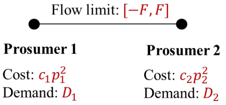
Mathematical Analysis: In this example, network constraint (5c) is simply $-F\leq-\lambda_{1}+b_{1}\leq F$. Given Prosumer 2’s strategy $b_{2}$, the price $\lambda_{1}$ solved from (5) is a function of $b_{1}$:

where the first and last scenarios correspond to cases in which the line flow reaches its lower and upper bound, respectively, and in the second scenario the line flow constraint is inactive. Prosumer 1’s decision-making problem is thus:

Given $b_{2}$, it can be verified that Prosumer 1’s objective (11) is continuous on $b_{1}\in\mathbb{R}$; moreover, it is linear and strictly decreasing on $(-\infty,~b_{2}-2F]$, quadratic and strictly convex on $(b_{2}-2F,~b_{2}+2F)$, and linear and strictly increasing on $[b_{2}+2F,~+\infty)$. Therefore, given $b_{2}$, the best response $b_{1}$ of prosumer 1 depends on the relationship between the axis of symmetry and the boundary points $(b_{2}\pm 2F)$ of the quadratic segment in its objective function. Specifically:

Similarly, given $b_{1}$, the best response of prosumer 2 is:

For any GNE $(\bar{p},\bar{b})$, its $(\bar{b}_{1},\bar{b}_{2})$ must fall in one of the following scenarios exclusively: $(P1M)~\&~(P2M)$, or $(P1U)~\&~(P2L)$, or $(P1L)~\&~(P2U)$, while all the other scenarios lead to contradiction. These three scenarios correspond to the three cases of GNEs as shown below. In particular, for scenario $(P1U)~\&~(P2L)$, one must have:

Similar conditions can be derived for scenarios $(P1L)~\&~(P2U)$, and $(P1M)~\&~(P2M)$. Therefore,

$\bullet$ If $|D_{1}-D_{2}|<(2c+1)F/c$:

and $\bar{p}_{i}=D_{i}+\bar{\lambda}_{i}-\bar{b}_{i}$ for $i=1,2$. It can be verified that $(\bar{p},\bar{b})$ is the unique GNE in this case. Moreover, $(\bar{p}_{1},\bar{p}_{2})$ coincides with the optimal solution of (10).

$\bullet$ If $D_{1}-D_{2}\geq(2c+1)F/c$, then every $(\bar{p},\bar{b})$ that satisfies:

and $\bar{p}_{i}=D_{i}+\bar{\lambda}_{i}-\bar{b}_{i}$ for $i=1,2$ is a GNE. Line congestion occurs since $D_{1}-\bar{p}_{1}=F=-(D_{2}-\bar{p}_{2})$, and there are a range of GNEs which have the same $\overline{p}$ that is optimal for (10).

$\bullet$ If $D_{1}-D_{2}\leq-(2c+1)F/c$, then every $(\bar{p},\bar{b})$ that satisfies:

and $\bar{p}_{i}=D_{i}+\bar{\lambda}_{i}-\bar{b}_{i}$ for $i=1,2$ is a GNE. Line congestion occurs since $-(D_{1}-\bar{p}_{1})=F=D_{2}-\bar{p}_{2}$, and there are a range of GNEs which have the same $\overline{p}$ that is optimal for (10). $\hfill\qed$

Economics Intuition: In this example, the only difference between two prosumers lies in the required energy reductions $D_{1}$ and $D_{2}$. This difference offers room for energy sharing. When $|D_{1}-D_{2}|$ is large, no matter which bid they start with, at some point during the bidding process the line will be congested with the power flow fixed. Take Prosumer 1 as an example and suppose $-\lambda_{1}+b_{1}$ is fixed to $-F$, then according to (11), it can constantly lower its total cost by offering a larger $b_{1}$ as long as the line is still congested. When Prosumer 1 increases its bid $b_{1}$ to an extreme, there is one GNE. With different starting points, there will be multiple GNEs. When the gap $|D_{1}-D_{2}|$ is small, the line will not be congested and thus, the prosumers do not have market power to manipulate the prices, and the bidding converges to a unique GNE.

The two-bus example above shows some nice properties of GNE(s) of game $\mathcal{G}$ in (7), such as existence and optimality in terms of (10), as well as uniqueness if no congestion occurs at the optimal solution of (10). However, these properties cannot be readily extended to general networks, as counter-examples are identified with the following three-prosumer model.

Example 2: Three prosumers are connected as shown in Fig. 3. Set $a=1$, $c_{1}=c_{2}=c_{3}=c$, $d_{1}=d_{2}=d_{3}=0$, $E_{i}^{0}=D_{i},\forall i=1,2,3$, and flow limit $F$ for the line connecting prosumers 1 and 2.

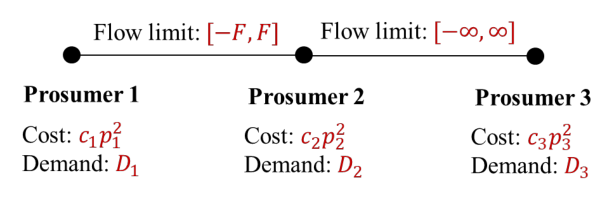
The GNE(s) for the three-prosumer example can be analyzed in a way similar to the two-prosumer example, although details are more involved and thus elaborated in Appendix C. In summary, if both lower and upper line flow constraints are inactive at the unique optimal solution of (10), then game $\mathcal{G}$ in (7) may either have no GNE or a unique GNE $(\bar{p},\bar{b})$ where $\bar{p}$ is optimal for (10). If one side of the line flow constraints is binding at the unique optimal solution of (10), then game $\mathcal{G}$, in general, may have no GNE or uncountably many GNEs; in the latter case, some of the GNEs have the same power profile $\bar{p}$ which is optimal for (10), while others do not. There are also special cases in which the game has a unique GNE: one example is that a line flow constraint is barely reached but not binding; another example is that a line flow constraint is binding and network parameters are just set on the boundary between no-GNE and multi-GNE cases. These special cases are rare in practice and hence not discussed in detail.

The two examples above show that for game $\mathcal{G}$ (7) in general, there is no guarantee for existence, uniqueness, or optimality of GNE, which exerts challenges on market operation. To tackle this problem, we develop an improved energy sharing mechanism with price regulation in Section IV.

We regulate energy sharing price of prosumer $i\in\mathcal{I}$ as:

where $\lambda_{i}(b)$ is the $i$-th element of the optimal solution of problem (5) given $b$. The regulated price (12) leads to an improved energy sharing mechanism described by the following decision-making problem for every prosumer $i\in\mathcal{I}$:

where

Remark: An implication of the price regulation policy (12) is that it restricts the price privilege granted to every prosumer $i\in\mathcal{I}$ compared to its marginal production adjustment cost. Formally, the price privilege of prosumer $i$ is $2c_{i}p_{i}+d_{i}-\lambda_{i}^{r}$ if it is a buyer ($q_{i}=D_{i}-p_{i}\geq 0$) and $\lambda_{i}^{r}-(2c_{i}p_{i}+d_{i})$ if it is a seller ($q_{i}<0$). With price regulation, the maximum price privilege of prosumer $i$ is restricted to $|q_{i}|/{a(I-1)}$, which can be regarded as prosumer $i$’s degree of participation in sharing characterized by its sharing amount $|q_{i}|$, market sensitivity factor $a$, and the total number $I$ of prosumers.

In the following, we show that the improved energy sharing mechanism (with price regulation) has desired properties.

The proof of Theorem 1 is in Appendix E. It shows that by including a price regulation policy, a unique GNE of the improved energy sharing mechanism always exists, which circumvents the no-GNE and multi-GNE issues encountered by the original game (7). Besides, the improved mechanism provides a simpler model for GNE computation by establishing equivalence between GNE and the optimal solution of (10).

The following proposition shows that every prosumer is incentivized to participate in the improved energy sharing market by incurring a cost not exceeding self-sufficiency.

Proposition 3 is proved in Appendix F. It shows that prosumer $i\in\mathcal{I}$’s cost in the energy sharing market is no more than its cost under self-sufficiency. Essentially, the improved sharing mechanism achieves a Pareto improvement over self-sufficiency and thus leaves no prosumer worse off. Thus, prosumer $i\in\mathcal{I}$ always has the incentive to implement $q_{i}$ as requied by the platform. A contract can be signed beforehand that prosumers who are not responding accordingly will face a high penalty or be barred from the market. If one prosumer has an equipment failure, we can exclude that prosumer from the energy sharing market and let the other prosumers bid again. We will show later that it only takes a few seconds for the proposed bidding algorithm to converge to a new equilibrium.

Welfare loss occurs at the GNE of the improved energy sharing game compared to the social optimum. Our next proposition quantifies and bounds this loss by price of anarchy.

Since the improved energy sharing game (13) has a unique GNE, which is also the “worst” equilibrium, its PoA equals the ratio between $J(\bar{p})$ and $J(\tilde{p})$. The proof of Proposition 4 is in Appendix G. It implies $\lim_{I\rightarrow\infty}\mbox{PoA}(I)=1$, i.e., the total disutility of prosumers at the GNE of the improved energy sharing game approaches the social optimum as the number of prosumers increases. In other words, the improved mechanism can still achieve social optimum in a large market as the original mechanism (as proved in Proposition 1).

The energy sharing price in our improved mechanism has an elegant structure as presented by the following proposition.

The proof of Proposition 5 is in Appendix H. The price $\bar{\lambda}_{i}^{r}$ in (17) is composed of $-\bar{\kappa}$, the price for network-wide energy balancing, and $-\sum_{l=1}^{L}\pi_{il}\bar{\tau}_{l}^{-}+\sum_{l=1}^{L}\pi_{il}\bar{\tau}_{l}^{+}$, the price of line congestion incident to prosumer $i\in\mathcal{I}$. This structure is similar to the classic locational marginal price (LMP) [42].

The price structure (17) implies that no subsidy is required to run the proposed energy sharing market, because the net sharing payment of all the prosumers at GNE is nonnegative as calculated below (where $\bar{\lambda}:=\bar{\lambda}^{r}=\lambda(\bar{b})$):

References

- [1] M. F. Akorede, H. Hizam, and E. Pouresmaeil, “Distributed energy resources and benefits to the environment,” Renewable and sustainable energy reviews, vol. 14, no. 2, pp. 724–734, 2010.
- [2] S. Salinas, M. Li, P. Li, and Y. Fu, “Dynamic energy management for the smart grid with distributed energy resources,” IEEE Transactions on Smart Grid, vol. 4, no. 4, pp. 2139–2151, 2013.
- [3] Y. Parag and B. K. Sovacool, “Electricity market design for the prosumer era,” Nature energy, vol. 1, no. 4, pp. 1–6, 2016.
- [4] Y. Ryu and H.-W. Lee, “A real-time framework for matching prosumers with minimum risk in the cluster of microgrids,” IEEE Transactions on Smart Grid, 2020.
- [5] W. Wei, F. Liu, and S. Mei, “Energy pricing and dispatch for smart grid retailers under demand response and market price uncertainty,” IEEE transactions on smart grid, vol. 6, no. 3, pp. 1364–1374, 2014.
- [6] T. Sousa, T. Soares, P. Pinson, F. Moret, T. Baroche, and E. Sorin, “Peer-to-peer and community-based markets: A comprehensive review,” Renewable & Sustainable Energy Reviews, vol. 104, pp. 367–378, 2019.
- [7] S. Benjaafar, G. Kong, X. Li, and C. Courcoubetis, “Peer-to-peer product sharing: Implications for ownership, usage, and social welfare in the sharing economy,” Management Science, p. mnsc.2017.2970, 2018.
- [8] Y. Chen, W. Wei, F. Liu, Q. Wu, and S. Mei, “Analyzing and validating the economic efficiency of managing a cluster of energy hubs in multi-carrier energy systems,” Applied energy, vol. 230, pp. 403–416, 2018.
- [9] W. Tushar, T. K. Saha, C. Yuen, T. Morstyn, H. V. Poor, R. Bean et al., “Grid influenced peer-to-peer energy trading,” IEEE Transactions on Smart Grid, vol. 11, no. 2, pp. 1407–1418, 2019.
- [10] N. Liu, X. Yu, C. Wang, and J. Wang, “Energy sharing management for microgrids with pv prosumers: A stackelberg game approach,” IEEE Transactions on Industrial Informatics, vol. 13, no. 3, pp. 1088–1098, 2017.
- [11] N. Liu, M. Cheng, X. Yu, J. Zhong, and J. Lei, “Energy-sharing provider for PV prosumer clusters: A hybrid approach using stochastic programming and stackelberg game,” IEEE Transactions on Industrial Electronics, vol. 65, no. 8, pp. 6740–6750, 2018.
- [12] S. Cui, Y.-W. Wang, and N. Liu, “Distributed game-based pricing strategy for energy sharing in microgrid with pv prosumers,” IET Renewable Power Generation, vol. 12, no. 3, pp. 380–388, 2017.
- [13] L. Chen, N. Liu, and J. Wang, “Peer-to-peer energy sharing in distribution networks with multiple sharing regions,” IEEE Transactions on Industrial Informatics, 2020.
- [14] X. Xu, J. Li, Y. Xu, Z. Xu, and C. S. Lai, “A two-stage game-theoretic method for residential pv panels planning considering energy sharing mechanism,” IEEE Transactions on Power Systems, 2020.
- [15] T. Morstyn and M. D. McCulloch, “Multiclass energy management for peer-to-peer energy trading driven by prosumer preferences,” IEEE Transactions on Power Systems, vol. 34, no. 5, pp. 4005–4014, 2018.
- [16] F. Moret, P. Pinson, and A. Papakonstantinou, “Heterogeneous risk preferences in community-based electricity markets,” European Journal of Operational Research, 2020.
- [17] L. Chen, N. Liu, L. Liu, X. Yu, and Y. Xue, “Data-driven stochastic game with social attributes for peer-to-peer energy sharing,” IEEE Transactions on Smart Grid, vol. 12, no. 6, pp. 5158–5171, 2021.
- [18] L. Han, T. Morstyn, and M. McCulloch, “Incentivizing prosumer coalitions with energy management using cooperative game theory,” IEEE Transactions on Power Systems, vol. 34, no. 1, pp. 303–313, 2018.
- [19] J. Mei, C. Chen, J. Wang, and J. L. Kirtley, “Coalitional game theory based local power exchange algorithm for networked microgrids,” Applied energy, vol. 239, pp. 133–141, 2019.
- [20] P. Chakraborty, E. Baeyens, K. Poolla, P. P. Khargonekar, and P. Varaiya, “Sharing storage in a smart grid: A coalitional game approach,” IEEE Transactions on Smart Grid, vol. 10, no. 4, pp. 4379–4390, 2018.
- [21] L. Han, T. Morstyn, and M. McCulloch, “Estimation of the shapley value of a peer-to-peer energy sharing game using coalitional stratified random sampling,” arXiv preprint arXiv:1903.11047, 2019.
- [22] M. J. Albizuri, H. Díez, and A. Sarachu, “Monotonicity and the aumann–shapley cost-sharing method in the discrete case,” European Journal of Operational Research, vol. 238, no. 2, pp. 560–565, 2014.
- [23] L. Han, T. Morstyn, C. Crozier, and M. McCulloch, “Improving the scalability of a prosumer cooperative game with k-means clustering,” in 2019 IEEE Milan PowerTech. IEEE, 2019, pp. 1–6.
- [24] J. N. Tsitsiklis and Y. Xu, “Efficiency loss in a cournot oligopoly with convex market demand,” Journal of Mathematical Economics, vol. 53, pp. 46–58, 2014.
- [25] N. Li, L. Chen, and M. A. Dahleh, “Demand response using linear supply function bidding,” IEEE Transactions on Smart Grid, vol. 6, no. 4, pp. 1827–1838, 2015.
- [26] Y. Xu, N. Li, and S. H. Low, “Demand response with capacity constrained supply function bidding,” IEEE Transactions on Power Systems, vol. 31, no. 2, pp. 1377–1394, 2015.
- [27] R. Johari and J. N. Tsitsiklis, “Parameterized supply function bidding: Equilibrium and efficiency,” Operations research, vol. 59, no. 5, pp. 1079–1089, 2011.
- [28] T. Morstyn, A. Teytelboym, and M. D. McCulloch, “Bilateral contract networks for peer-to-peer energy trading,” IEEE Transactions on Smart Grid, vol. 10, no. 2, pp. 2026–2035, 2018.
- [29] Y. Chen, S. Mei, F. Zhou, S. H. Low, W. Wei, and F. Liu, “An energy sharing game with generalized demand bidding: Model and properties,” IEEE Transactions on Smart Grid, vol. 11, no. 3, pp. 2055–2066, 2020.
- [30] Y. Chen, C. Zhao, S. H. Low, and S. Mei, “Approaching prosumer social optimum via energy sharing with proof of convergence,” IEEE Transactions on Smart Grid, vol. 12, no. 3, pp. 2484–2495, 2020.
- [31] D. Kalathil, C. Wu, K. Poolla, and P. Varaiya, “The sharing economy for the electricity storage,” IEEE Transactions on Smart Grid, vol. 10, no. 1, pp. 556–567, 2017.
- [32] J. Barquín and M. Vázquez, “Cournot equilibrium calculation in power networks: An optimization approach with price response computation,” IEEE transactions on power systems, vol. 23, no. 2, pp. 317–326, 2008.
- [33] L. Xu and R. Baldick, “Transmission-constrained residual demand derivative in electricity markets,” IEEE Transactions on Power Systems, vol. 22, no. 4, pp. 1563–1573, 2007.
- [34] J. Yao, S. S. Oren, and I. Adler, “Two-settlement electricity markets with price caps and cournot generation firms,” european journal of operational research, vol. 181, no. 3, pp. 1279–1296, 2007.
- [35] Y. Liu and F. F. Wu, “Impacts of network constraints on electricity market equilibrium,” IEEE Transactions on Power Systems, vol. 22, no. 1, pp. 126–135, 2007.
- [36] H. Le Cadre, P. Jacquot, C. Wan, and C. Alasseur, “Peer-to-peer electricity market analysis: From variational to generalized nash equilibrium,” European Journal of Operational Research, vol. 282, no. 2, pp. 753–771, 2020.
- [37] J. Guerrero, A. C. Chapman, and G. Verbič, “Decentralized p2p energy trading under network constraints in a low-voltage network,” IEEE Transactions on Smart Grid, vol. 10, no. 5, pp. 5163–5173, 2018.
- [38] M. H. Albadi and E. F. El-Saadany, “Demand response in electricity markets: An overview,” in 2007 IEEE power engineering society general meeting. IEEE, 2007, pp. 1–5.
- [39] B. F. Hobbs, C. B. Metzler, and J.-S. Pang, “Strategic gaming analysis for electric power systems: An mpec approach,” IEEE transactions on power systems, vol. 15, no. 2, pp. 638–645, 2000.
- [40] P. T. Harker, “Generalized nash games and quasi-variational inequalities,” European journal of Operational research, vol. 54, no. 1, pp. 81–94, 1991.
- [41] G. Scutari, D. P. Palomar, F. Facchinei, and J.-S. Pang, “Monotone games for cognitive radio systems,” in Distributed decision making and control. Springer, 2012, pp. 83–112.
- [42] S. Bose and S. H. Low, “Some emerging challenges in electricity markets,” in Smart Grid Control. Springer, 2019, pp. 29–45.
- [43] J. Hirshleifer, A. Glazer, and D. Hirshleifer, Price theory and applications: decisions, markets, and information. Cambridge University Press, 2005.
- [44] S. Boyd, N. Parikh, E. Chu, B. Peleato, J. Eckstein et al., “Distributed optimization and statistical learning via the alternating direction method of multipliers,” Foundations and Trends® in Machine learning, vol. 3, no. 1, pp. 1–122, 2011.
- [45] W. Wei, F. Liu, S. Mei, and Y. Hou, “Robust energy and reserve dispatch under variable renewable generation,” IEEE Transactions on Smart Grid, vol. 6, no. 1, pp. 369–380, 2014.
- [46] P. Samadi, H. Mohsenian-Rad, R. Schober, and V. W. Wong, “Advanced demand side management for the future smart grid using mechanism design,” IEEE Transactions on Smart Grid, vol. 3, no. 3, pp. 1170–1180, 2012.
- [47] W. Wu, J. Chen, B. Zhang, and H. Sun, “A robust wind power optimization method for look-ahead power dispatch,” IEEE transactions on sustainable energy, vol. 5, no. 2, pp. 507–515, 2014.
- [48] B. Stott, J. Jardim, and O. Alsaç, “Dc power flow revisited,” IEEE Transactions on Power Systems, vol. 24, no. 3, pp. 1290–1300, 2009.
- [49] D. Singh, D. Singh, and K. Verma, “Multiobjective optimization for dg planning with load models,” IEEE transactions on power systems, vol. 24, no. 1, pp. 427–436, 2009.
- [50] C. Su, “Equilibrium problems with equilibrium constraints: Stationarities, algorithms, and applications.” 2004.
- [51] M. Fukushima, “Theory of nonlinear optimization,” Sangyo Tosho, 1980.
- [52] G. Still, “Lectures on parametric optimization: An introduction,” 2018.
Appendix A Proof of Proposition 1
First, we prove that a unique optimal solution of (8) exists. The construction of the matrix after equation (4) implies boundedness of the feasible set (8b)–(8b) for . Indeed, that construction leads to:
where , . and are obtained by removing the last prosumer from vectors and . Multiplying both sides by implies boundedness of , and further boundedness of due to being a constant. Hence, the strictly convex objective function (8a) attains a unique optimal solution in the compact convex set (8b)–(8c).
Problem (8) can be rewritten as