Ballistic-to-hydrodynamic transition and collective modes
for two-dimensional electron systems in magnetic fieldPreprint: APS/123-QED
Abstract
The recent demonstrations of viscous hydrodynamic electron flow in two-dimensional electron systems poses serious questions to the validity of existing transport theories, including the ballistic model, the collision-induced and collisionless hydrodynamics. While the theories of transport at hydrodynamic-to-ballistic crossover for free 2d electrons are well established, the same is not true for electrons in magnetic fields. In this work, we develop an analytically solvable model describing the transition from ballistic to hydrodynamic transport with changing the strength of electron-electron collisions in magnetic fields. Within this model, we find an expression for the high-frequency non-local conductivity tensor of 2d electrons. It is valid at arbitrary relation between frequency of external field , the cyclotron frequency , and the frequency of e-e collisions . We use the obtained expression to study the transformation of 2d magnetoplasmon modes at hydrodynamic-to-ballistic crossover. In the true hydrodynamic regime, , the 2DES supports a single magnetoplasmon mode that is not split at cyclotron harmonics. In the true ballistic regime, , the plasmon dispersion develops splittings at cyclotron harmonics, forming the Bernstein modes. A formal long-wavelength expansion of kinetic equations (”collisionless hydrodynamics”) predicts the first splitting of plasmon dispersion at . Still, such expansion fails to predict the zero and negative group velocity sections of true magnetoplasmon dispersion, for which the full kinetic model is required.
I Introduction
In common semiconductor materials, scattering of electrons by phonons and impurities leads to the diffusive Ohmic transport. At the same time, in pure materials, the characteristic momentum relaxation length for scattering by phonons and impurities can exceed the size of the device . This leads to ballistic dc transport with predominant scattering of electrons at the sample boundaries Mayorov et al. 2011a; Heremans et al. 1992a. A very interesting situation appears when momentum-conserving electron-electron collisions are intense, so that the respective free path and . In this case, electrons form a viscous fluid with its dynamics described by the Navier-Stokes equations. This corresponds to the hydrodynamic dc transport, where current whirlpools and negative nonlocal resistance Gurzhi 1968; Levitov and Falkovich 2016; Torre et al. 2015; Pellegrino et al. 2016; Chandra et al. 2019a can be observed. This hydrodynamic regime in electronic systems has attracted significant interest and has been experimentally demonstrated in graphene Bandurin et al. 2016; Kumar et al. 2017; Bandurin et al. 2018; Berdyugin et al. 2019; Ku et al. 2020, (Al,Ga)As heterostructures Braem et al. 2018, GaAs quantum wells Gusev et al. 2018; Gusev et al. 2021 and Weyl semimetals Gooth et al. 2017; Gooth et al. 2018; Osterhoudt et al. 2021.
The parameter space for diffusive, ballistic, and hydrodynamic regimes changes at finite frequency of external field . A number of interesting effects in ac transport was predicted theoretically for ideal electron fluid Moessner et al. 2018; Semenyakin and Falkovich 2018; Cohen and Goldstein 2018; Alekseev 2018 where e-e collisions are so intense that . The ballistic regime in this case refers to a model of a collisionless electron plasma that is valid for describing processes that occur in times shorter than the free path of electrons ( and ) or for processes whose characteristic spatial scales are smaller than the free path lengths (, , where - characteristic wave vector of wave processes) Aleksandrov et al. 1978. In many experimentally relevant situations, particularly, at THz or GHz frequencies, and are comparable in magnitude. This leads to the need to construct models of the transport intermediate between hydrodynamic and ballistic regimes Müller et al. 2009; Müller et al. 2008; Narozhny et al. 2015; Foster and Aleiner 2009; Svintsov et al. 2012; Lucas et al. 2016; Mayorov et al. 2011b; Svintsov 2018; Chandra et al. 2019b; Holder et al. 2019; Gupta et al. 2021; Ledwith et al. 2019; Heremans et al. 1992b. It’s important to mention that ideal electron fluid is formed at very strong e-e collisions, contrary to ideal electron gas where electrons do not interact at all. Indeed, the dc kinematic viscosity ( is the Fermi velocity) tends to zero for very short free path time . On the other hand, the ballistic transport can be equivalently termed as ’highly viscous’. The true Navier-Stokes hydrodynamics is inapplicable in this regime. Yet it is possible to expand the transport equations in the long-wavelength limit, generating the nearly local ’collisionless hydrodynamics’ or ’hydrodynamics of highly viscous fluid’ in which the equations of motion can be interpreted as the Navier-Stokes equations. Aleksandrov et al. 1978; Alekseev 2018.
Such equations predict the existence of a novel collective mode, the transverce zero sound, in the absence of a magnetic field Lucas and Sarma 2018; Khoo and Villadiego 2019. In finite magnetic field , the dynamic viscosity was predicted to have the viscoelastic resonance Alekseev 2018; Alekseev and Alekseeva 2019; Alekseev 2019. The latter should occur at double cyclotron frequency . Interaction between 2d plasmons and viscoelastic resonance was predicted to lead to emergence of novel collective mode, dubbed as ”transverse zero magnetosound” Alekseev and Alekseeva 2019.
The predicted mode structure of highly non-ideal electron fluid contradicts to that of ballistic electrons, though both regimes should be equivalent and appear at . The ballistic theory states that plasmon dispersion interacts with multiple cyclotron resonances forming the so called Bernstein modes Chiu and Quinn 1974; Bernstein 1958; Sitenko and Stepanov 1957; Batke et al. 1985; Gudmundsson et al. 1995; Batke et al. 1986; Holland et al. 2004; Roldan et al. 2011; Volkov and Zabolotnykh 2014; Bandurin et al. 2022. The fundamental Bernstein mode, like conventional magnetoplasmon, starts from at . As it approaches , it reaches a plateau, and then falls downward with negative group velocity. The group velocity on the plateau is zero, and density of states is singular. The plateau frequency is shifted from by minigap. The next branch of the Bershtein modes starts from at and forms a plateau near the triple cyclotron frequency. Similar branches occur at each multiple of the cyclotron frequency.
In this article, we are aiming to resolve the abovementioned contradictions between ’ballistic’ and ’highly-viscous hydrodynamic’ models for 2DES in magnetic field. To this end, we develop a generalized classical kinetic model that describes magnetotransport in ballistic and hydrodynamic transport regimes as limiting cases (with ). The model is based on Boltzmann kinetic equation with model momentum and particle conserving e-e collision integral. We calculate the nonlocal high-frequency conductivity with non-zero magnetic field, which is a necessary block for calculating many light-matter interaction characteristics Ciracì et al. 2012; Gonçalves et al. 2021; Lundeberg et al. 2017a (Section II).
Using the expression for conductivity, we study the evolution of the dispersion of magnetoplasmons during the transition from the hydrodynamic regime to the ballistic regime (Section III). At a high frequency of electron-electron collisions corresponding to the hydrodynamic regime, an conventional magnetoplasmon with a single cyclotron gap is observed. As the collision frequency decreases, more and more pronounced dispersion splittings at multiple cyclotron frequencies appear, which in the ballistic regime take on the explicit form of Berstein modes. We inspect the approximation of ”collisionless” hydrodynamics (Section IV) and find that is applicable only for wave vectors smaller than the anticrossing point of the two lowest Bernstein modes, coinciding with them in the region of applicability. This means that transverse zero magnetosound is an artifact of long-wave expansion of transport equations beyond the region of applicability.

II Non-local high frequency conductivity tensor
We start with evaluation of the non-local conductivity tensor of 2DES in a classically strong perpendicular magnetic field . To this end, we find the current response in a weak electric field with . It is found from the solution of linearized kinetic equation
| (1) |
where distribution function , is the electron velocity, the speed of light and the electron-electron collision integral. In a practically important limit in which the electron-phonon scattering can be neglected Narozhny et al. 2021, only electrons with velocities close to the Fermi velocity participate in high-frequency kinetic processes, which makes this model applicable for describing both classical 2DES and graphene. Contrary to electron-impurity and electron-phonon collisions, e-e collisions conserve the net momentum of colliding particles. To account for this fact, we adopt the e-e collision integral in generalized relaxation-time approximation Svintsov 2018; Abrikosov and Khalatnikov 1959; Bhatnagar et al. 1954; Gross and Krook 1956; Mermin 1970; Lucas and Hartnoll 2018; Guo et al. 2017; Lucas 2017. The collision integral pushes the distribution function towards local equilibrium
| (2) |
where and are found from the conservation of particle number and momentum:
| (3) |
The kinetic equation with e-e collision integral (2) and conservation laws (3) are sufficient to describe the behaviour of electron liquid at large wave vectors , and across the whole hydrodynamic-to-ballistic crossover. The scheme of solution is described in Appendix A. First, one passes to the polar coordinates in momentum space and expands the distribution function in Fourier series. Physically, the coefficients of these series are cyclotron harmonics. The kinetic equation in cyclotron harmonic representation is purely algebraic. Its symbolic solution at the first stage contains two unknown variables, and . On the second stage, these ’hydrodynamic quantities’ are found from the conservation laws (3). In a practically important limit , this leads us to a system of linear equations describing both ballistic and hydrodynamic behavior of 2DES:
| (4) |
where is the dimensionless collision frequency, the Fermi velocity, equilibrium carrier density and . The dimensionless factors
| (5) |
where is the -th order derivative of the Bessel function, a cyclotron radius and a cyclotron frequency.
These equations can be interpreted as generalized hydrodynamics; the term ’generalized’ implies applicability at arbitrarily large wave vectors. When expanded to terms (with ), we obtain ”collisionless” hydrodynamics () or ”true” hydrodynamics ():
| (6) |
| (7) |
where the ac shear viscosity coefficients and depend on magnetic field and frequency as
| (8) | |||
| (9) |
where is the viscosity in the absence of magnetic field. Whereas ”true” hydrodynamics, due to the small relaxation time, is also valid for large wave vectors, collisionless hydrodynamics has a limited range of applicability () which requires special care when applying this approximation for large wave vectors.
Finally, the components of the conductivity tensor can be found from
| (10) |
where the relation between and is found from equations (4) .
It is instructive to track the changes in longitudinal conductivity while varying the strength of e-e collisions. Fig.1 illustrates this evolution and shows the frequency dependence of at fixed and THz. In the ballistic regime ( ps, blue curve), the conductivity has resonances at multiple cyclotron frequencies which amplitude decreases with increasing the resonance order. As the frequency of e-e collisions becomes comparable to , multiple resonances rapidly fade away. Only the main cyclotron resonance persists in the hydrodynamic regime, and its width shrinks again at very short values of , i.e. at low viscosity.
III Magnetoplasmon dispersion

We proceed to inspect the evolution of collective excitations in magnetized 2DES across the hydrodynamic-ballistic crossover. To address this problem, we consider the excitation of collective modes by a point dipole located above the 2DES in the quasi-static regime (). We find that total electric potential in the 2DES plane can be represented as (Appendix B):
| (11) |
where is the electric potential of the point source in the absence of 2DES and the 2DES dielectric function. In the quasi-static regime, it is affected only by the longitudinal component of the conductivity tensor and is given by
| (12) |
where is the effective dielectric constant, the distance to the gate electrode located below the 2DES and the longitudinal conductivity was obtained before in Sec. II.
It is convenient to visualize the dispersion of plasmons using the loss function . The peaks in loss function correspond to a resonant enhancement of external electric field, i.e. to the collective electrostatic waves – (magneto)plasmons. Using the obtained generalized equations of hydrodynamics, it is possible to trace the evolution of collective modes with an increase in the frequency of electron-electron collisions up to the transition to the hydrodynamic regime.
The emerging loss functions are displayed in Fig. 2. Our calculations show that the splittings of plasmon dispersion at multiple cyclotron frequencies are gradually blurred with increasing e-e collision frequency . In the hydrodynamic regime, the dispersion collapses into an ordinary magnetoplasmon
| (13) |
where .

Now it’s important to track the transition from the obtained results to the zero magnetic field. In the absence of a magnetic field in the ballistic regime, the phase velocity of plasmons does not fall below the Fermi velocity in Dirac materials; thus, the dispersion of plasmons does not fall into the Landau damping region, and at low values of the carrier density and a low gate distance , the dispersion asymptotically tends to the boundary Svintsov 2018; Lundeberg et al. 2017b. However, in the presence of a weak magnetic field, this boundary is destroyed due to the splitting of the Bershtein modes (Fig. 3)

IV Collisionless hydrodynamic model
In this section, we study the range of applicability of collisionless hydrodynamics for the description of magnetoplasmon modes. Using the continuity equation (6) and the Navier-Stokes equations (7), we find the conductivity of a two-dimensional system by definition (10). We plot the loss function in the collisionless hydrodynamic model (6-7) and in the ballistic transport model (4) (Fig.4). In the first one (Fig.4a) the zeros of the dielectric function (12) in this case give two magnetoplasmon modes. The first of them goes from the cyclotron frequency , at small wave vectors it coincides with the conventional magnetoplasmon (13), and at large wave vectors (after the anti-crossing point ) it coincides with the transverse magnetosound
| (14) |
which is related to perturbations of shear stress of a charged Fermi liquid in a magnetic field. Alekseev and Alekseeva 2019 The second mode starts from the doubled cyclotron frequency and after the anti-crossing point tends to conventional magnetoplasmon. It is possible to approximately estimate the anti-crossing point as the point at which the value of doubled cyclotron frequency is reached by the dispersion of conventional magnetoplasmon (13):
| (15) |
In this case, up to the anti-crossing point , there is a good agreement with the two lowest Bernstein modes observed in the full theory (Fig.4b) (but modes starting at multiple cyclotron frequencies are not observed). However, for large wave vectors, serious discrepancies are observed. In the collisionless hydrodynamics model, the lowest mode exceeds twice the cyclotron frequency and coincides with the magnetosonic mode, while in the full theory, the fundamental Bernstein mode never exceeds twice the cyclotron frequency and forms a plateau with a singular density of states.
V Discussion and conclusion
In the limit , the constructed full kinetic theory describes Bernstein modes. Magnetosound waves predicted in the framework of collisionless hydrodynamics described by the equations (7) in Ref. Alekseev and Alekseeva 2019 coincide with the full theory only in a narrow -range. Since the lowest mode in the collisionless hydrodynamics model tends to magnetosound mode (14) only after the anti-crossing point (15), where this model is inapplicable, it can be argued that transverse magnetosound modes are an artifact of spectrum cutoff in generalized hydrodynamic equations (4) and are not observed in the full theory.
While the physics behind these differences is clear, it’s interesting to see and compare the emerging absorption spectra. The dielectric function corresponds to the screening by electrons of the two-dimensional system of the external field (Appendix B). The loss function Im is responsible for the magnetoplasmon-assisted absorption. It peaks at the magnetoplasmon modes, and therefore should enhance the near-field magnetoabsorption of an inhomogeneous field incident on the 2DES. Bandurin et al. 2022
Both transverse magnetosound and Bernstein modes are predicted in the loss function (Fig.4). In both cases, for pure materials, an asymmetric (with respect to the magnetic field) resonance enhancement of magnetoabsorption in the vicinity of the doubled cyclotron frequency is predicted. However, in the case of magnetosound, the sharp side of the resonance is located in the direction of high magnetic fields, and in the case of Bershtein modes, on the contrary, in the direction of low magnetic fields, which makes it possible to distinguish one from the other in measurements.
Measurements of the photoresistence demonstrate similar asymmetric resonances at double, triple, and even quadruple the cyclotron frequency in pure graphene in a magnetic field Bandurin et al. 2022 that matches the Bernstein modes seen in the full theory and are not predicted by the model of collisionless hydrodynamics. In the full theory the sharp side of the resonance is located in the direction of low magnetic fields. In Ref. Alekseev and Alekseeva 2019 it was shown for a thin strip of a 2DES in the case of collisionless hydrodynamics that the sharp side of the resonance is located in the direction of high magnetic fields. However, the shape of the resonance strongly depends on the width of the strip and becomes almost symmetric in the case of an infinite 2DES. It can be assumed that in this case the shape of the resonance should strongly depend on the shape of the sample. However, measurements of various samples show an asymmetry consistent with the full theory Dai et al. 2010; Bandurin et al. 2022, which is another argument that these resonances are caused by Bernstein modes.
In summary, a model of high-frequency dynamics of a two-dimensional electronic system has been constructed, which allows one to study the transition from the ballistic regime to the hydrodynamic. It is shown that the conventional magnetoplasmon in the hydrodynamic regime, with a decrease in the frequency of electron-electron collisions, acquires characteristic splittings at multiple cyclotron frequencies and becomes Bernstein modes in the ballistic limit. According to calculations, the model of ”collisionless” hydrodynamics, which predicts transverse magnetosound, is applicable to the description of magnetoplasmon modes only for wave vectors not exceeding the anti-crossing point (15) of the two lowest Berstein modes, and magnetosound mode are beyond the range of applicability of this model.
Acknowledgements.
The work was supported by grant # 21-12-00287 of the Russian Science FoundationAppendix A: Solution of the kinetic equation
To solve the kinetic equation (1), we pass to polar coordinates (with ) and represent the equation as:
| (16) |
where , , , and is the cyclotron frequency. Then, we seek for the function in the form , and expand as a series of angular harmonics :
Appendix B: Magnetoabsorption calculation
In this section, we first consider the absorption of an inhomogeneous wave by an infinite two-dimensional electron system, then consider the case when an inhomogeneous field is created by planar charge density located a short distance from the plane of a 2DES () (Fig.5). The absorption given by the Joule’s law:
| (19) |
where is the total field in the plane of the two-dimensional system. Further, we take into account the Ohm’s law with conductivity tensor
| (20) |
and obtain an expression for the absorbed power in the form
| (21) |
In the plane of a two-dimensional system, the field is screened by electrons of 2DES. In the electrostatic approximation (), suitable for describing a sharp increase in absorption by a strongly inhomogeneous Bernstein mode field, the total potential in the plane of the system is given by the expression
| (22) |
where is the dielectric function and substrate dielectric constant.
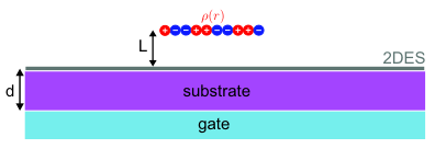
To find the dielectric function of a planar symmetric non-gated two-dimensional system with a known conductivity tensor , we solved the field equation (with )
| (23) |
where and . Solving the obtained equations, we obtain an expression for the dielectric function
| (24) |
Taking into account the screening by a gate located at a distance , we obtain the expression (12)
In this case, the expression for absorption takes the form
| (25) |
The specific type of charge density depends on the problem. Absorption caused by an inhomogeneous field of charges resulting from the diffraction of an incident plane wave on a thin contact was considered in detail in Ref. Bandurin et al. 2022
References
- Mayorov et al. (2011a) A. S. Mayorov, R. V. Gorbachev, S. V. Morozov, L. Britnell, R. Jalil, L. A. Ponomarenko, P. Blake, K. S. Novoselov, K. Watanabe, T. Taniguchi, et al., Nano letters 11, 2396 (2011a).
- Heremans et al. (1992a) J. Heremans, M. Santos, and M. Shayegan, Applied physics letters 61, 1652 (1992a).
- Gurzhi (1968) R. Gurzhi, Soviet Physics Uspekhi 11, 255 (1968).
- Levitov and Falkovich (2016) L. Levitov and G. Falkovich, Nature Physics 12, 672 (2016).
- Torre et al. (2015) I. Torre, A. Tomadin, A. K. Geim, and M. Polini, Physical Review B 92, 165433 (2015).
- Pellegrino et al. (2016) F. M. Pellegrino, I. Torre, A. K. Geim, and M. Polini, Physical Review B 94, 155414 (2016).
- Chandra et al. (2019a) M. Chandra, G. Kataria, D. Sahdev, and R. Sundararaman, Physical Review B 99, 165409 (2019a).
- Bandurin et al. (2016) D. Bandurin, I. Torre, R. K. Kumar, M. B. Shalom, A. Tomadin, A. Principi, G. Auton, E. Khestanova, K. Novoselov, I. Grigorieva, et al., Science 351, 1055 (2016).
- Kumar et al. (2017) R. K. Kumar, D. Bandurin, F. Pellegrino, Y. Cao, A. Principi, H. Guo, G. Auton, M. B. Shalom, L. A. Ponomarenko, G. Falkovich, et al., Nature Physics 13, 1182 (2017).
- Bandurin et al. (2018) D. A. Bandurin, A. V. Shytov, L. S. Levitov, R. K. Kumar, A. I. Berdyugin, M. B. Shalom, I. V. Grigorieva, A. K. Geim, and G. Falkovich, Nature communications 9, 1 (2018).
- Berdyugin et al. (2019) A. I. Berdyugin, S. Xu, F. Pellegrino, R. K. Kumar, A. Principi, I. Torre, M. B. Shalom, T. Taniguchi, K. Watanabe, I. Grigorieva, et al., Science 364, 162 (2019).
- Ku et al. (2020) M. J. Ku, T. X. Zhou, Q. Li, Y. J. Shin, J. K. Shi, C. Burch, L. E. Anderson, A. T. Pierce, Y. Xie, A. Hamo, et al., Nature 583, 537 (2020).
- Braem et al. (2018) B. A. Braem, F. Pellegrino, A. Principi, M. Röösli, C. Gold, S. Hennel, J. V. Koski, M. Berl, W. Dietsche, W. Wegscheider, et al., Physical Review B 98, 241304 (2018).
- Gusev et al. (2018) G. Gusev, A. Levin, E. Levinson, and A. Bakarov, Physical Review B 98, 161303 (2018).
- Gusev et al. (2021) G. Gusev, A. Jaroshevich, A. Levin, Z. Kvon, and A. Bakarov, Physical Review B 103, 075303 (2021).
- Gooth et al. (2017) J. Gooth, A. C. Niemann, T. Meng, A. G. Grushin, K. Landsteiner, B. Gotsmann, F. Menges, M. Schmidt, C. Shekhar, V. Süß, et al., Nature 547, 324 (2017).
- Gooth et al. (2018) J. Gooth, F. Menges, N. Kumar, V. Sü, C. Shekhar, Y. Sun, U. Drechsler, R. Zierold, C. Felser, and B. Gotsmann, Nature communications 9, 1 (2018).
- Osterhoudt et al. (2021) G. B. Osterhoudt, Y. Wang, C. A. Garcia, V. M. Plisson, J. Gooth, C. Felser, P. Narang, and K. S. Burch, Physical Review X 11, 011017 (2021).
- Moessner et al. (2018) R. Moessner, P. Surówka, and P. Witkowski, Physical Review B 97, 161112 (2018).
- Semenyakin and Falkovich (2018) M. Semenyakin and G. Falkovich, Physical Review B 97, 085127 (2018).
- Cohen and Goldstein (2018) R. Cohen and M. Goldstein, Physical Review B 98, 235103 (2018).
- Alekseev (2018) P. Alekseev, Physical Review B 98, 165440 (2018).
- Aleksandrov et al. (1978) A. F. Aleksandrov, L. S. Bogdankevich, and A. A. Rukhadze, Moscow Izdatel Vysshaia Shkola (1978).
- Müller et al. (2009) M. Müller, J. Schmalian, and L. Fritz, Physical review letters 103, 025301 (2009).
- Müller et al. (2008) M. Müller, L. Fritz, and S. Sachdev, Physical Review B 78, 115406 (2008).
- Narozhny et al. (2015) B. Narozhny, I. Gornyi, M. Titov, M. Schütt, and A. Mirlin, Physical Review B 91, 035414 (2015).
- Foster and Aleiner (2009) M. S. Foster and I. L. Aleiner, Physical Review B 79, 085415 (2009).
- Svintsov et al. (2012) D. Svintsov, V. Vyurkov, S. Yurchenko, T. Otsuji, and V. Ryzhii, Journal of Applied Physics 111, 083715 (2012).
- Lucas et al. (2016) A. Lucas, R. A. Davison, and S. Sachdev, Proceedings of the National Academy of Sciences 113, 9463 (2016).
- Mayorov et al. (2011b) A. S. Mayorov, R. V. Gorbachev, S. V. Morozov, L. Britnell, R. Jalil, L. A. Ponomarenko, P. Blake, K. S. Novoselov, K. Watanabe, T. Taniguchi, et al., Nano letters 11, 2396 (2011b).
- Svintsov (2018) D. Svintsov, Physical Review B 97, 121405 (2018).
- Chandra et al. (2019b) M. Chandra, G. Kataria, D. Sahdev, and R. Sundararaman, Physical Review B 99, 165409 (2019b).
- Holder et al. (2019) T. Holder, R. Queiroz, T. Scaffidi, N. Silberstein, A. Rozen, J. A. Sulpizio, L. Ella, S. Ilani, and A. Stern, Physical Review B 100, 245305 (2019).
- Gupta et al. (2021) A. Gupta, J. Heremans, G. Kataria, M. Chandra, S. Fallahi, G. Gardner, and M. Manfra, Physical Review Letters 126, 076803 (2021).
- Ledwith et al. (2019) P. Ledwith, H. Guo, A. Shytov, and L. Levitov, Phys. Rev. Lett. 123, 116601 (2019).
- Heremans et al. (1992b) J. Heremans, M. Santos, and M. Shayegan, Applied physics letters 61, 1652 (1992b).
- Lucas and Sarma (2018) A. Lucas and S. D. Sarma, Physical Review B 97, 115449 (2018).
- Khoo and Villadiego (2019) J. Y. Khoo and I. S. Villadiego, Physical Review B 99, 075434 (2019).
- Alekseev and Alekseeva (2019) P. Alekseev and A. Alekseeva, Physical review letters 123, 236801 (2019).
- Alekseev (2019) P. Alekseev, Semiconductors 53, 1367 (2019).
- Chiu and Quinn (1974) K. Chiu and J. Quinn, Physical Review B 9, 4724 (1974).
- Bernstein (1958) I. B. Bernstein, Physical Review 109, 10 (1958).
- Sitenko and Stepanov (1957) A. Sitenko and K. Stepanov, Soviet Phys. JETP 4 (1957).
- Batke et al. (1985) E. Batke, D. Heitmann, J. Kotthaus, and K. Ploog, Physical review letters 54, 2367 (1985).
- Gudmundsson et al. (1995) V. Gudmundsson, A. Brataas, P. Grambow, B. Meurer, T. Kurth, and D. Heitmann, Physical Review B 51, 17744 (1995).
- Batke et al. (1986) E. Batke, D. Heitmann, and C. Tu, Physical Review B 34, 6951 (1986).
- Holland et al. (2004) S. Holland, C. Heyn, D. Heitmann, E. Batke, R. Hey, K. Friedland, and C.-M. Hu, Physical review letters 93, 186804 (2004).
- Roldan et al. (2011) R. Roldan, M. Goerbig, and J.-N. Fuchs, Physical Review B 83, 205406 (2011).
- Volkov and Zabolotnykh (2014) V. Volkov and A. Zabolotnykh, Physical Review B 89, 121410 (2014).
- Bandurin et al. (2022) D. A. Bandurin, E. Mönch, K. Kapralov, I. Y. Phinney, K. Lindner, S. Liu, J. H. Edgar, I. A. Dmitriev, P. Jarillo-Herrero, D. Svintsov, and S. D. Ganichev, Nature Physics (2022).
- Ciracì et al. (2012) C. Ciracì, R. Hill, J. Mock, Y. Urzhumov, A. Fernández-Domínguez, S. Maier, J. Pendry, A. Chilkoti, and D. Smith, Science 337, 1072 (2012).
- Gonçalves et al. (2021) P. Gonçalves, T. Christensen, N. M. Peres, A.-P. Jauho, I. Epstein, F. H. Koppens, M. Soljačić, and N. A. Mortensen, Nature communications 12, 1 (2021).
- Lundeberg et al. (2017a) M. B. Lundeberg, Y. Gao, R. Asgari, C. Tan, B. Van Duppen, M. Autore, P. Alonso-González, A. Woessner, K. Watanabe, T. Taniguchi, et al., Science 357, 187 (2017a).
- Narozhny et al. (2021) B. Narozhny, I. Gornyi, and M. Titov, Physical Review B 103, 115402 (2021).
- Abrikosov and Khalatnikov (1959) A. Abrikosov and I. Khalatnikov, Reports on Progress in Physics 22, 329 (1959).
- Bhatnagar et al. (1954) P. L. Bhatnagar, E. P. Gross, and M. Krook, Physical review 94, 511 (1954).
- Gross and Krook (1956) E. P. Gross and M. Krook, Physical Review 102, 593 (1956).
- Mermin (1970) N. D. Mermin, Physical Review B 1, 2362 (1970).
- Lucas and Hartnoll (2018) A. Lucas and S. A. Hartnoll, Physical Review B 97, 045105 (2018).
- Guo et al. (2017) H. Guo, E. Ilseven, G. Falkovich, and L. S. Levitov, Proceedings of the National Academy of Sciences 114, 3068 (2017).
- Lucas (2017) A. Lucas, Physical Review B 95, 115425 (2017).
- Lundeberg et al. (2017b) M. B. Lundeberg, Y. Gao, R. Asgari, C. Tan, B. Van Duppen, M. Autore, P. Alonso-González, A. Woessner, K. Watanabe, T. Taniguchi, et al., Science 357, 187 (2017b).
- Dai et al. (2010) Y. Dai, R. Du, L. Pfeiffer, and K. West, Physical review letters 105, 246802 (2010).