Rotation measure and synchrotron emission signatures in simulations of magnetized galactic discs2021Rotation measure and synchrotron emission signatures in simulations of magnetized galactic discs–15
Abstract
We analyse observational signatures of magnetic fields for simulations of a Milky-Way like disc with supernova-driven interstellar turbulence and self-consistent chemical processes. In particular, we post-process two simulations data sets of the SILCC Project for two initial amplitudes of the magnetic field, 3 and 6 G, to study the evolution of Faraday rotation measures (RM) and synchrotron luminosity. For calculating the RM, three different models of the electron density are considered. A constant electron density, and two estimations based on the density of ionized species and the fraction of the total gas, respectively. Our results show that the RM profiles are extremely sensitive to the models, which assesses the importance of accurate electron distribution observations/estimations for the magnetic fields to be probed using Faraday RMs. As a second observable of the magnetic field, we estimate the synchrotron luminosity in the simulations using a semi-analytical cosmic ray model. We find that the synchrotron luminosity decreases over time, which is connected to the decay of magnetic energy in the simulations. The ratios between the magnetic, the cosmic ray, and the thermal energy density indicate that the assumption of equipartition does not hold for most regions of the ISM. In particular, for the ratio of the cosmic ray to the magnetic energy the assumption of equipatition could lead to a wrong interpretation of the observed synchrotron emission.
Keywords:
ISM: magnetic fields – ISM: cosmic rays – radio continuum: ISM – ISM: kinematics and dynamics – galaxies: ISM – galaxies: magnetic fields1 Introduction
Magnetic fields are ubiquitous in the universe. They are observed at a wide range of spatial scales and field strengths; the average magnetic field strength on the surface of Earth is about G (Hulot et al. 2010; Guyodo & Valet 1999) and on the Sun about G (Scherrer et al. 1977), while it can reach several thousand Gauss in sun spots (e.g. Jurčák et al. 2018; Schmassmann et al. 2018). Entire (spiral) galaxies are magnetized with ordered magnetic fields of typically to G (e.g. Beck 2001; Beck et al. 2012; Beck 2015a; Krause et al. 2018). Galaxy clusters and the intracluster medium also show evidence of magnetic fields of the microgauss order (Han 2017; Stuardi et al. 2021). The study of magnetic fields is a central part of astrophysical research. One reason is that their influence and involvement in many processes is now well established. For example, the magnetic fields of spiral galaxies could influence the star formation rate (Krumholz & Federrath 2019). They also play a role in cosmic ray (CR) propagation (Zweibel 2013; Zweibel 2017; Shukurov et al. 2017), and are a main driver of stellar activity (Landstreet 1992; Berdyugina 2005).
Magnetic field amplification in many astrophysical systems is often explained by dynamo activity (Brandenburg & Subramanian 2005). In spiral galaxies, for instance, the - dynamo can convert kinetic energy from to differential rotation and turbulence into magnetic energy (Beck 2015a). However, magnetic fields aligned with the galaxy’s differential rotation axis have a characteristic strength of the order of one micrograuss (Naab & Ostriker 2017, e.g.) which cannot be explained by the - dynamo alone since the amplification time characteristic of this process is much longer than the age of the system itself (Ruzmaikin et al. 2013). Therefore, additional dynamo processes should be involved to reach the observed magnetic field strengths in galaxies, such as the small-scale turbulent dynamo (Brandenburg et al. 2012a; Brandenburg et al. 2012b; Schober et al. 2013). This phenomenon amplifies magnetic fields on scales smaller than the characteristic injection scale of turbulence that is primarily driven by supernova (SN) explosions in the interstellar medium. An exhaustive literature on the small-scale dynamo as the main mechanism for the amplification of magnetic fields in the interstellar medium is available (see for example Rieder & Teyssier 2016, Gent et al. 2021).
To distinguish different scenarios of magnetic field generation, reliable observational tracers of astrophysical magnetic fields are needed. Many observational techniques allow to obtain various information on the structure and strength of the fields. The Faraday rotation measure (RM), for example, allows to determine the magnetic field’s projection along the line of sight, by analyzing the rotation of the polarization plane of electromagnetic waves coming from radio sources located in the background or within the observed environment (Enßlin & Vogt 2003; Frick et al. 2011; Bhat & Subramanian 2013). The measurement of polarized synchrotron emission makes it possible to study the component normal to the line of sight, as well as to estimate the total intensity of the field (Orlando et al. 2009). However, since the observed quantities are usually field projections, the reconstruction of the exact spatial structure of the magnetic field remains a significant challenge (e.g. Beck et al. 2019; Seifried et al. 2020; Girichidis 2021). Indeed, the computation of the RM requires to know the distribution of thermal electrons, and the estimation of the three-dimensional structure of the field from radio observations requires to measure the Stokes parameters and to involve Faraday tomography (Brentjens & de Bruyn 2005, e.g.). Synchrotron emission is emitted by relativistic charged particles that travel in the interstellar magnetic field is the second observable. However, extracting the magnetic field from synchrotron observation requires an assumption on the power spectrum of the cosmic rays (Blumenthal & Gould 1970, e.g.).
Despite a constant improvement of the theoretical tools describing the dynamics of astrophysical plasmas, difficulties are encountered in the attempt to match observations to theoretical models. The need for detailed numerical modelling of the interstellar medium (ISM) then becomes a necessity. Some of the most detailed simulations of the magnetized turbulent Milky Way ISM are presented in the SILCC project11 1 Official webpage: https://hera.ph1.uni-koeln.de/~silcc/ (Walch et al. 2015; Girichidis et al. 2016). The central aim of the SILCC simulations is the analysis of the formation and evolution of molecular clouds, as well as their dynamical characteristics. Specifically, they carry out an in-depth study on the influence of stellar feedback, like supernovae, on the evolution of the ISM. The magnetohydrodynamical simulations cover the ISM in different phases (ionized, atomic and molecular) from K down to K with densities ranging from . Girichidis et al. 2018b (data release 6, DR6) focus on the magnetic field, which allows a detailed comparison of the field properties in different phases of the ISM (see also Pardi et al. 2017, for comparable models in periodic boxes of the local SN-driven ISM).
The objective of this paper is the implementation and analysis of two observables of the magnetic field to the SILCC simulation set, in order to probe the sensitivity of typical assumption made in the reconstruction of magnetic fields from radio observations. In a first step, we will study the dynamics of the Faraday rotation over the simulation time for different models of the electron density. In a second step, we will use the model for the cosmic-ray electrons developed by Schober et al. 2016, to post-process the simulation data, in order to study the time evolution of the synchrotron luminosity. Additionally, we will calculate the energy density of cosmic rays and magnetic fields as well as the thermal energy in order to test the equipartition between these components. The structure of this paper is organized as follows. In Sec. 2, we briefly review the simulations from the SILCC project. In Sec. 3, we compute Faraday rotation measures for the simulations from the SILCC project (DR6), in particular by implementing different distribution models for the free electrons. In Sec. 4, we present the synchrotron emission model applied to the DR6 simulations, and the evolution of the energy densities. Conclusions and perspectives are discussed in Sec. 5.
2 Simulation data
2.1 The DR6 simulation set
We post-process simulations from the SILCC project (SImulating the Life Cycle of molecular Clouds; Walch et al. 2015; Girichidis et al. 2016). The physics modules and the simulation setup are described in detail in Walch et al. 2015. The effects of magnetic fields have been investigated in Girichidis et al. 2018b and were published as data release 6 (DR6). Below we summarize the main simulation features.
The simulation setup covers a stratified box with a size of . The setup uses periodic boundary conditions along and and diode boundary conditions along the stratification axis , which means the gas can leave but not enter the simulation box. The equations of ideal MHD are solved using the HLLR5 solver (Bouchut et al. 2007; Bouchut et al. 2010; Waagan 2009; Waagan et al. 2011) in the adaptive mesh refinement (AMR) code Flash22 2 Version 4, http://flash.uchicago.edu/site/ (Fryxell et al. 2000; Dubey et al. 2008). Radiative cooling and heating of the gas are coupled to the evolution of the non-equilibrium abundances using a chemical network. The hydrogen and carbon chemistry including the abundances of ionized (H+), atomic (H) and molecular (H2) hydrogen as well as carbon monoxide (CO) and singly ionized carbon follows Glover & Mac Low 2007, Micic et al. 2012, and Nelson & Langer 1997. Molecular cooling follows the description in Glover et al. 2010 and Glover & Clark 2012. For temperatures above , equilibrium abundances are assumed and the cooling based on Gnat & Ferland 2012 is employed. Heating of the gas includes spatially clustered supernovae (SNe), which is described in more detail below, cosmic ray (Goldsmith & Langer 1978) and X-ray (Wolfire et al. 1995) heating as well as photoelectric heating (Bakes & Tielens 1994; Bergin et al. 2004; Wolfire et al. 2003). The constant interstellar radiation field with a strength of (Habing 1968; Draine 1978) is locally attenuated in dense shielded regions. The local column depth is computed using the TreeCol algorithm (Clark et al. 2012), which has been implemented and optimized for Flash as described in Wünsch et al. 2018. The dust-to-gas mass ratio is set to 0.01 with dust opacities based on Mathis et al. 1983 and Ossenkopf & Henning 1994.
The initial gas distribution follows a Gaussian profile with a scale height of and a central density of , which yields a total gas column density of . The temperature is adjusted such that the gas is initially in pressure equilibrium. This corresponds to a central temperature of and a value of at large altitudes, where a lower boundary to the density () is applied.
Besides self-gravity an external potential is included that accounts for the stellar component of the disc. An isothermal sheet is used (Spitzer 1942) with a stellar gas surface density of and a vertical scale height of . The gravitational forces are computed using the tree-based method described in Wünsch et al. 2018.
The initial magnetic field is oriented along the direction. The central field strength in the midplane at is set to in one simulation and to in a second run and scales vertically with the density, . An initial small scale tangled perturbation of the field is not included. The mass-to-flux ratio (measured along the direction) of the entire box is approximately in units of the critical value , i.e., the disc as a whole is not supported by the magnetic pressure. The initial conditions of a field parallel to the midplane is motivated by observations of the Milky Way.
Stellar feedback is included as a temporally constant SN rate. The Kennicutt-Schmidt relation (Kennicutt 1998) is used to find a star formation rate based on the total gas column density of the simulation box. The star formation rate is then converted to a SN rate assuming the initial stellar mass function from Chabrier 2003. This results in a rate of approximately for the box. A distinction is made between a type Ia component (20% of the SNe) with a uniform distribution in and directions and a Gaussian distribution in direction with a scale height of and a type II component (the remaining 80% of the SNe) with a vertical scale height of . The latter are further split into a runaway component (40%) of individual explosions and a clustered component (60%), which are grouped in clusters with sizes ranging from 7 to 40 SNe per cluster. We note that this simplified treatment of stellar feedback is lacking self-consistent star formation and additional direct feedback from localised star clusters like stellar winds and radiation (Gatto et al. 2017; Rathjen et al. 2021, see, e.g.). However, the inclusion of Lagrangian sink particles as a representation of star clusters to accurately follow the star formation and feedback includes an ad-hoc treatment of the magnetic field for the accretion of gas from the grid to the particles. We therefore restrict our analysis to these simplified models.
The grid is initialized at a resolution of cells. The adaptive mesh refinement further increases the resolution by a factor of four, i.e. an effective resolution of cells with a cell size of . For the post-processing, we extract the data as a uniform grid at the highest resolution, namely grid cells. We use data snapshots from to Myr with a constant time step of Myr. A discussion about the effect of resolution on the final results of our analysis is presented in Appendix B.
2.2 Magnetic field evolution
Figure 1 shows the time evolution of the different components of the magnetic field for the two simulations with initial volume-weighted strengths of and 6 G, respectively. Initially, the magnetic field increases mainly due to adiabatic compression of the field caused by supernovae explosions and gravitational contraction. The and components of the magnetic field are initially zero. In both runs, increases initially, but then decays after Myr. The components and show a similar evolution for the run with G, but in the run with G they are amplified in the first Myr, before decaying. On the other hand, we observe that the arithmetic mean , decreases progressively for the two different values of and that and are close to zero over the entire simulation time.
These different behaviors can be explained by the following arguments. Girichidis et al. 2018b have shown that the magnetic field amplitude scales with the total gas density in the following way: for low density and weak magnetic fields , while for zones with a density close to the mean density of the ISM ( g cm-3), . Since supernova-driven turbulence creates dense zones via converging flows, an amplification of the magnetic energy then becomes consistent with the evolution of the rms average of the different components of the field. The fact that and oscillate close to 0 can be explained by the isotropy of the field, caused by randomly placed supernovae. Finally, the decay of magnetic energy, mainly due to the combination of supernovae explosions that tend to disperse gas across the domain, is also in line with our interpretation. Figure 12 in the appendix shows the evolution of the individual energies for completeness as well as the total mass in the simulation box. For a detailed discussion of the energies and the outflows we refer the reader to Girichidis et al. 2018b.
3 Faraday rotation measures
3.1 Methodology
3.1.1 Basic equations
A linearly polarized electromagnetic wave travelling through a medium with a characteristic size and a magnetic field parallel to the propagation of the wave undergoes rotation of its polarization plane with a characteristic rotation angle
| (1) |
Here, is the wavelength, is the initial angle of the polarization plane, and
| (2) |
is called the rotation measure (or Faraday depth) with rad m-2 cm3 G-1 pc-1, where , and are the charge and mass of the electron, and the speed of light, respectively.
In our analysis, we consider an ideal situation in the sense that each pixel of a RM map has a radio source in the background, and we take into account neither any broadening process, nor the effects of multiple sources on the Faraday spectrum (for more details, see for example Brentjens & de Bruyn 2005).
3.1.2 Data treatment
We use the YT software package (Turk et al. 2011) to analyse the simulations. To calculate RM, we discretize formula (2) to give
| (3) |
where is the parallel component of the magnetic field to the axis along which the RM is estimated and is the size of a grid cell. For a cubic numerical domain of dimension , there are possible lines of sight (LOS) that can be calculated on the plane perpendicular to each Cartesian axis, namely , , and . For extracting the different data, we map the original grid with adaptive mesh refinement onto a uniform grid with a resolution of . Finally, the RM is calculated according to formula (3).
Equation (2) implies that a completely random configuration of the magnetic field will lead to a (plane) average of
| (4) |
where the sum is performed over all lines of sight of a given plane. Therefore, we will also calculate the rms value of the RM:
| (5) |
Obviously, the rms-calculation process could in itself present a number of drawbacks; if zones with strong magnetic fields (or high electron density) form, they will significantly increase the RM value (a concrete example will be presented in Sec. 3.2). In particular, intuitive information about the structure of the field (or at least the inversion structure of the RM values) is lost, because the square of each is considered (see equation 5). Therefore, comparing those two averages can give us indications about structural properties of the magnetic field. Furthermore, we also consider the following estimator:
| (6) |
which measures the deviation between the highest value of RM and its plane average. We will use this quantity as an indicator of the (possible) existence of high-RM zones that could lead to an increase in . The definitions of the plane average as given in Eq. (4), the rms as given in Eq. (5), and the estimator given in Eq. (6) will be applied for other quantities in simulations as well.
Another useful quantity that we analyse is called the dispersion measure (DM) and is defined as:
| (7) |
The DM basically gives information about the projected electron density, and could also tell us if high-value RM and DM patches are observed in the same region, which could indicate that the electron density might have a greater influence on the RM than magnetic field variations. Averages and the estimator of DM are defined in the same way as for RM.
Finally, to study typical length scales of various quantities, such as the RM maps and the free electron density, we calculate power spectra. For a given physical quantity , we define its correlation function as:
| (8) |
where is the position vector between two points, and where the average is performed over all possible points . Considering an isotropic system, the latter quantity only depends on . Taking the Fourier transform of the last expression, we can write:
| (9) |
where
| (10) |
and where is the power spectrum of . The power spectrum is then averaged over all -shells with a constant wavenumber amplitude, in order to obtain a one-dimensional profile33 3 For the numerical calculation we use the python package scipy.fft (Cooley & Tukey 1965).. Note that formula (9) can be applied either to three-dimensional data, as well as weight-projected two-dimensional maps.
3.1.3 Thermal electron density models
In this section we present three different electron density models that are implemented in the calculation of the rotation measure. The objective of considering multiple density models is to test the response of the Faraday signal, and then establish if offset RM values are observed between, for example, a basic model of constant electron density and a more complex model, accounting for the gas dynamics of the ISM. Assuming a constant electron density for performing an RM analysis is not uncommon in the literature, especially in numerical simulations. We can cite, as an example, the (nearly) incompressible simulations conducted by Bhat & Subramanian 2013 in order to study the Faraday signal in the framework of the small-scale dynamo, assuming a constant electron density because of the small variations of the latter. So in order to test the effect of more complex distribution of electron density on the RM, we will consider the following models:
- •
model 1. First, we consider the most trivial situation where the thermal electron distribution is constant, and where its value is set to cm-3. Given formula (3), only the magnetic fields should directly influence the rotation measure.
- •
model 2. Here, the thermal electron density is computed via the mass fraction of the ionized species implemented in the simulations (C+ and H+). If is the carbon mass fraction with respect to the total gas density, the contribution to electron density from ionized carbon will be given as , where is the mass of carbon in atomic mass units. The total electron density will be given by (where is calculated with the same procedure).
- •
model 3. Lastly, we make the hypothesis that the electron density can be written in the form or equivalently , where is the total particle density expressed in cm-3, and is a proportionality factor. In particular, is obtained by dividing the mass density times the mass fraction of each species by their corresponding mass , i.e.:
(11) In this work, we will use which results in values of that are, on average, of the same order of magnitude as the ones obtained from models 1 and 2.
Figure 2 shows the evolution of the electron density for models 2 and 3. Both the rms and the average of model 2 are approximately constant over time, as is the average of model 3. In contrast, the rms for model 3 increases by more than an order of magnitude between about and Myr, and then becomes constant. This is directly linked to the fact that model 3 takes into account all chemical species in the calculation of the electron density. Indeed, the zones of overdensity (due to shock waves from supernova explosions) tend to raise the rms value, the average value being unchanged or even very little influenced because these areas of high density are limited to small regions of space compared to the size of the simulation box.
3.2 Resulting rotation measure evolution in the simulations
In Fig. 3 we show the time evolution of , , and in the three rows from top to bottom. The three models are shown from left to right for the two simulations with and 6 G, respectively.
For the model 1 (left panels), it is not surprising to see that the mean and rms values of the RM evolve similarly to the magnetic field presented in Fig. 1, because this model uses a constant electron density (fixed at cm-3). The estimator decreases during the entire simulation time (except for a small peak during the earliest times). Along the and -axes, is almost constant during the entire simulation, with an average value around . Along the axis, it constantly decreases over time, with a maximum value of at 5 Myr. This is mainly due to the fact that the magnetic field is initialized along the axis (decreasing exponential profile above and below the galactic plane), and it progressively spreads out in the simulation domain, loosing the initial disc-like shape, causing less variations between the average value of the magnetic field in the simulation box and its maximum value.
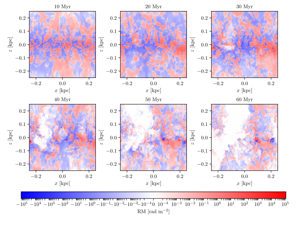
The model 2 shows a different evolution. The value of along the and axes is approximately zero during the entire simulation time, which may indicate the isotropic character of the components of the magnetic field reached in particular because of the gas mixing. On the other hand, along the axis, decreases over time to reach approximately zero at the end of the simulation, which is also an effect of the gas mixing. A different evolution is observed for the rms value. A peak (of approximately 60–80 rad m-2, depending on the axis and the initial value considered) appears around 40 Myr. The presence of high-density zones of ionized species seems to be the origin of such a peak. Indeed, the curves present the same kind of evolution, reaching more than rad m-2 along the axis. Furthermore, the evolution of in Fig. 4 shows an increase up to 30–40 Myr, reaching approximately cm-2 at the end of the simulation. Furthermore, also increases during the whole simulation, supporting our hypothesis of the presence of high-density zones of ionized gas. Finally, looking at the RM spectra shown in Fig. 5 (only along the axis), it appears that the peaks of the spectra are increasingly shifted towards larger wave numbers (i.e. shorter characteristic length scales). Overall, the typical RM values (plane average and rms) of model 2 are about 10 to 20 times higher than those of model 1.
As mentioned before, in model 3, we have chosen to present only RM and DM results for the case . This value was introduced in a ad hoc manner in order to reproduce typical RM values that correspond approximately to those observed in the Milky Way (e.g. Taylor et al. 2009). Changing would only shift the curves vertically, and therefore would not alter the conclusions. Figure 3 shows that this model produces again different RM curves from the other two models discussed above. The evolution of is extremely similar in both models 2 and 3, except that the peaks observed at 40 Myr reach almost 300 rad m-2 (approximately four times the value observed in model 2). This may be due to the fact that the electron density is proportional to the total density of the gas, contrary to the model 2 which only takes into account the ionised species (C+ and H+). The average value of the rotation measure has stronger variations than the model 2 after 40 Myr, which can be attributed to faster gas dispersion caused by stronger values of the magnetic field. Thus, the conclusions drawn for model 2 can partly be applied here as well: the dense gas that is compressed by supernovae and gravity can strongly contribute to in this model. Note that the presence of such zones with dense gas can be seen in Fig. 6, which shows RM maps for different simulation times along the axis. Figure 5 shows the evolution of the RM power spectra for models 1, 2, and 3. In model 1, we observe that the spectra are peaked at the lowest wave numbers, which implies that the typical length-scale of RM patches is approximately the size of the simulation box. This is not surprising given that the thermal electron density is assumed to be constant. We also observe that the peak of the spectrum is progressively shifted towards higher wave numbers, due to the restructuring of the magnetic field. On the contrary, models 2 and 3 show the opposite trend; at early times, the spectra resulting from model 2 have peaks around which are progressively shifting towards the largest wave numbers, while for model 3, this trend is even more prominent (It appears nevertheless that the initial peaks of model 3 are more around , which can be simply explained by the fact that all of the chemical species are included in the calculation of in this model, and that the density of electrons can be more important in certain regions other than in model 2). The most probable explanation for such an observation is that the formation of regions with high electron density is formed by the SN-driven turbulence. Despite the fact that these power spectra only allow us to extract qualitative characteristics of the distribution of RM values, they are, in our case, a useful source of information allowing us to support our hypothesis that areas of high electron density are responsible for the different patterns observed between the thermal electron models.
3.3 Impact of the initial large-scale magnetic field on the Faraday signals
It should be noted that the initial conditions for the magnetic field in the SILCC simulation are simplified. It is initialized along the axis, that does not take into account the complexity of the magnetic field that could be observed in spiral galaxies. However, we argue that this condition should not affect our conclusions.
Observations of face-on spiral galaxies show the presence of a large-scale magnetic fields with a component following the direction of spiral arms (e.g. Beck 2015b). Therefore, considering a large-scale magnetic field along the -direction (the galactic plane lies in the -plane) should be a good approximation. Also, the simulation box is a cube of 500 pc edges, which is quite small compared to the overall size of the Milky Way (whose radius is though to be of the order of 20 kpc). Therefore any geometrical variations of the field should not be relevant at this scale. However, the observations reveal that the large-scale magnetic field is about ten times smaller than the random field, which is not reflected in the initial conditions.
However, the magnetic field evolves dynamically throughout the simulation and the field configuration is more realistic after approximately Myr. Therefore, our conclusions are only based on the data at times Myr. On the contrary, above approximately 45-50 Myr, a non negligible amount of gas has left the box, and the dynamics has altered the gas structure significantly.

4 Synchrotron emission
4.1 Theory and methods
4.1.1 Diffusion-loss equation for the cosmic ray power spectrum
The synchrotron luminosity is a second observable of the magnetic field in the ISM. Synchrotron emission is produced by cosmic ray electrons gyrating around magnetic fields. Since cosmic rays are not included in the DR6 data release of the SILCC simulations, we employ a semi-analytical model for the power spectrum of such electrons. We follow the approach adopted by Schober et al. 2016, but see also Werhahn et al. 2021a; Werhahn et al. 2021b; Werhahn et al. 2021c for a similar approach on galactic scales.
Our model includes two different populations of CR electrons. The primary population, which originates from supernovae remnants (meaning that electrons gain energy through Fermi acceleration processes) and the secondary electrons, which are created by proton-decay pion production. The general expression for the energy injection spectrum of a cosmic ray species is a power-law (Bell 1978) of the form
| (12) |
where is the normalization factor, is the energy of species (rest mass plus kinetic energy), and is the spectral index. Analytical models of cosmic ray acceleration predict a dependence of on the compression factor and characteristic velocities of the shock (Bell 1978). For typical shock parameters, these analytical models result in , but more detailed models of supernova shock fronts yield (Bogdan & Volk 1983; Lacki & Thompson 2012). We choose a value of for our study. The evolution of the spectrum for a cosmic ray species , , is governed by the diffusion-loss equation (Torres 2004, see e.g.)
| (13) |
where is the cooling rate, is the timescale for catastrophic losses, and is a spatial diffusion coefficient.
4.1.2 Primary CR electrons
In order to derive the steady state spectrum of primary electrons, Eq. (13) can be simplified by making the same assumptions as proposed in Lacki & Beck 2013. For a steady state, the time derivative in Eq. (13) vanishes. Additionally, one assumes spatial homogeneity of the ISM, and that catastrophic losses are negligible. The cooling rate is assumed to be of the form , where represents the typical cooling timescale of the CR electrons, involving various processes that will be described below. Therefore, Eq. (13) simply becomes:
| (14) |
After integrating the latter with respect to , we have
| (15) |
4.1.3 Secondary CR electrons and CR protons
In Eq. (15), the injection spectrum of CR electrons takes into account the contribution of both primary and secondary electrons, namely . However, using gamma-ray observations of M82 and NGC253, Lacki et al. 2011, Lacki & Beck 2013 estimated that the value of the ratio to be approximately 0.6-0.8. In this paper, we adopt . Therefore, we have . Following again the steps of Lacki & Beck 2013, we can relate to the power spectrum of CR protons . Note that the CR protons mainly suffer catastrophic losses via pions production. The typical life time of CR protons is with being the timescale of pion production. We set (Lacki & Beck 2013). Therefore, determining is sufficient to find the full expression of the CR electrons. The injection spectrum of CR protons is estimated as follows. We make the hypothesis that the protons only originate from supernovae explosions. Assuming a power-law expression of the form (12), and connecting to the supernova rate (see Schober et al. 2016), we can write the expression
| (16) |
where is the amount of supernovae energy transferred into energy of CR protons, is the supernova rate density with being the supernova rate per grid cell and the volume of a grid cell, and is the total energy released by a single supernova. We assume and erg. Integrating the latter equation and rearranging all the terms yields
| (17) |
Note that is derived according to how the probability of supernovae is implemented in the SILCC simulations (see Girichidis et al. 2018b), and we provide a detailed calculation of this term in Appendix C. The factor ensures to have the right units for . Finally, putting Eqns. (12), (15), and (17) together, we obtain
| (18) |
4.1.4 CR electron cooling timescale
In Eq. (18), the different cooling processes taken into account in the expression of are ionization (ion), bremsstrahlung (brems), inverse Compton scattering (IC), synchrotron emission (synch), and galactic winds (wind). Their expressions are given as follows:
| (19) | |||||
| (20) | |||||
| (21) | |||||
| (22) | |||||
| (23) |
where is the Thompson cross section, is the density of all neutral species implemented in the simulations (namely H, H2, and CO), is the density of ionized species (H+ and C+), is the energy density of the interstellar radiation field, is the energy density of the magnetic field, is the typical length scale of the simulation domain, and is the typical velocity of galactic winds. The ionisation formula comes from Schlickeiser 2002, and the bremsstrahlung expression comes from Strong & Moskalenko 1998. In , we adopt pc, which is the scale height at which the stellar component of the gas is initialized in the SILCC simulations. For the typical value of the galactic winds, we adopt km/s.
In order to derive the expression of the energy of the interstellar radiation field, we adopt the same approach as Schober et al. 2016. We consider four main components: the cosmic microwave background (CMB), infrared (IR), an optical component (opt) and finally an ultraviolet (UV) component (Winner et al. 2019; Winner et al. 2020, see also). If we assume that each of those components can be described by a Planck curve with the corresponding temperature, then the total energy density of thermal interstellar radiation is
| (24) |
with . The coefficients and the temperatures were estimated by Chakraborty & Fields 2013 and Cirelli & Panci 2009, and are summarized in Tab. 1.
| Process | ||
|---|---|---|
| UV | ||
| Optical | ||
| IR | 41 | |
| CMB | 1 |
Altogether, the general expression of the cooling timescale is given as:
| (25) |
Figure 7 shows histograms of the different cooling timescales given by Eqs. (19)–(23) in all grid cells, at and Myr and for cosmic ray energies of keV and GeV, for the run with G. Clearly, it appears that at 10 GeV, in most cells is determined by , which, in our model, does not depend on the energy of the cosmic rays and is constant in space and time. For lower energies, the dominant contribution to is ionisation. Furthermore, bremsstrahlung becomes relevant for later times, given the cooling timescale associated with this process depends on the density of ionized species, that are constantly created by the supernovae explosions. At GeV, given its dependency on the energy, the synchrotron emission starts to play a role (although not major) in the values of . The inverse Compton scattering has not yet crossed the value of , but it will likely take over the galactic winds as an upper limit of . As an example, Werhahn et al. 2021c modelled various cooling timescales for disc-like galaxies, implementing non-radiative (hadronic and Coulomb interactions of CRs with the interstellar medium) and radiative (synchrotron, inverse Compton, and bremsstrahlung) processes. They showed an example of typical cooling timescales value at 10 GeV (see Fig. 1 in Werhahn et al. 2021c). Each of these processes rarely has a characteristic timescale longer than approximately Myr. In our study, although those values seem to match the ones of our implemented processes, numerous grid cells reach extreme values that could go up to approximately Myr in the case of the synchrotron emission. At first glance, this is clearly due to the gas distribution of the simulations, which in our case create regions with extreme values of neutral (or ionized) gas densities. Our results show that the gas distribution in the ISM along with the choice of cooling processes governing the diffusion-loss equation of the cosmic rays are two major components that could impact the power spectrum of CR electrons to a large extent. Note that no major differences are observed with the case G (see Fig. 14 in the appendix), so all our analysis can apply to this case without any loss of generality.
4.1.5 Synchrotron luminosity
Using the work of Blumenthal & Gould 1970, the expression of the synchrotron power spectrum for a distribution of electrons is given by:
| (26) |
where
| (27) |
with being the Bessel function of the second kind with parameter is the power spectrum of a single electron, and where
| (28) |
The integral over the pitch angle is roughly equal to 8.9, for the specific value . Note that Schober et al. 2016 also added the contribution of free-free electron absorption/emission. However, with the typical values of the physical parameters we consider in our models, this contribution is negligible, and therefore not considered in our model.
4.1.6 Data treatment
As mentioned in Sec. 3.1.2, the resolution of the simulations is dynamically and locally adapted with respect to the gas density. In particular, corresponds to the resolution of the most refined regions in the simulations. We adopt the same strategy described in Sec. 3.1.2, and map all the data onto a uniform grid of grid cells, except for the data corresponding to Myr, for which the resolution is fixed at . In particular, this means that less refined regions are simply volume-weight averaged. In order to work on two-dimensional maps, we reduce the three-dimensional data in the following way. For a given physical quantity (given as an output of the simulations), we calculate the weighted average
| (29) |
where pc is the size of the simulation domain and is the size of a grid cell. Given that our data are mapped onto a uniform grid, Eq. (29) simply reduces to the sum of along a given axis. By convention, we perform our analysis along the axis, meaning that we work with the plane, being the vertical coordinate from the disc plane. We apply then Eq. (29) to the components of the magnetic field, and to gas fractions of the different chemical species involved in the dynamics of the simulations.
The synchrotron luminosity (26) is directly calculated on averaged two-dimensional maps. In particular, we calculate the quantity that will be presented in units of solar luminosity erg s-1. For quantitative comparison, we create a one-dimensional profile for maps of a physical quantity of interest as follows. Once a projected map is created according to formula (29), we take the average value, using the same formula (4) for the average of rotation measure maps, of each horizontal line (corresponding to a fixed coordinate above/below the galactic midplane). As an example, for calculating the vertical profile of the magnetic field amplitude, we project each magnetic field component , and along a given axis ( axis across the midplane by convention), we create the map of the projected magnetic field as , and then we take the average value of each horizontal line. This process could be applied to any physical quantity that is given as an output of the simulations.
4.2 Resulting synchrotron luminosity in the simulations

Figure 8 shows an example of the evolution of synchrotron luminosity maps, in the plane, for the run with G. We observe that the typical values of the luminosity globally decrease with time. Additionally, the highest values seem to be correlated with the density of the gas. Indeed, it can be observed on the Myr map that most of the synchrotron luminosity is concentrated in the center of the galactic mid-plane. On the other hand, we cannot exclude that the synchrotron luminosity is mostly influenced by the value of the magnetic field, which would be more in line with our intuition. A first indication is given in Fig. 9, which shows the time evolution of one-dimensional profiles of the magnetic field, the cosmic ray number density given by
| (30) |
where is given by Eq. (18), the gas total density, and the synchrotron luminosity. It becomes then more evident that the decrease of the synchrotron luminosity is rather connected to the evolution of the magnetic field than the other quantities. Indeed, it appears that the average gas density does not vary significantly in time, while the and rms values increase (which clearly indicates that denser regions are created by shock waves following supernova explosions).
Another hint is provided by Fig. 10, were we show the vertical profiles of and of the magnetic field. The vertical structure seems to be extremely similar, which tends also to disclose any other quantities than the magnetic field to influence the synchrotron luminosity. These results suggest that our model is not strongly dependent on the physical processes participating in the cooling of CR electrons described in Sec. 4.1.4, that are rather sensitive to the different chemical species numerical densities.
In conclusion, there is a strong evidence that the evolution of the synchrotron luminosity is mostly determined by variations of the magnetic field. It is therefore probable that considering models of cosmic ray electrons with less, additional or other cooling processes than those entering the expression of (see Eq. 25) would not result in huge variations in the resulting synchrotron maps. However, a deeper analysis of the sensitivity of the synchrotron emission to different CR models will be the focus of future work.
As it has been mentioned before, the choice to set pc has been motivated by the fact that this value was actually the scale height at which the stellar component was initialized in the SILCC simulations (Girichidis et al. 2018b). With a typical velocity for the galactic winds of km/s, this leads to a cooling timescale around Myr, which is quite short compared to typical values that are estimated for the Milky Way. Furthermore, it is also clear that the value of should not stay constant over time; the vertical structure will change in time which should modify both values of and . In this sense, the vertical disc dynamics should play an important role in the simulations and they could, in principle, change the overall luminosity of the simulation box. However, the SILCC simulations are conducted over 60 Myr, which is relatively short time compared to the typical time scales of the Milky Way’s dynamics, which could justify our choice to use a constant cooling time scale.
Additionally, we have computed the synchrotron luminosity (26) by setting . The results are shown as blue curves on Fig. 9. In absence of galactic winds, the cosmic ray number density is approximately one order of magnitude higher than our fiducial model. The synchrotron luminosity shows the same trend, but being approximately half an order of magnitude higher without wind. In this sense, we can state that any value chosen between the extreme case of Myr and would not produce significant bias in the final results of synchrotron luminosity, and that our conclusions will not suffer from this choice of parameter. Of course, a more thorough investigation must be conducted in order to study the influence of a more complex vertical disc dynamics on the resulting synchrotron emission, which is reserved for a future work.
4.3 Equipartition between cosmic rays and magnetic energies
The assumption of energy equipartition between the magnetic field and the cosmic ray electrons is often used in the analysis of synchrotron radiation. However, this assumption has important limitations due to the possibly fundamentally different temporal and spatial evolution of the two energy densities, see, e.g., Beck & Krause 2005 and Seta & Beck 2019. Whereas on global galactic scales the assumption of energy equipartition might be reasonable, the local deviations from it on scales below kiloparsecs can be significant. Numerical simulations of the interstellar medium including non-equilibrium cooling and cosmic ray protons in the advection-diffusion approximation suggest that the CR energy density on scales from a few up to pc only vary by a factor of a few (Girichidis et al. 2018a, see, e.g.). On the contrary, the magnetic field energy scales with the density (Crutcher 2012; Hennebelle & Inutsuka 2019, e.g.) and thus varies by orders of magnitudes in different regions of the simulation box. The additional complication of different production channels for CR protons and electrons in combination with the vastly different cooling efficiencies challenges the assumption of equipartition.
In order to examine the exact energy density distribution of the CR electrons and the other energy components, one needs to include accurate CR electron processes including the formation of primaries and secondaries, which is not included in the current simulations (see e.g. Werhahn et al. 2021a; Werhahn et al. 2021b; Werhahn et al. 2021c, for a post-processing treatment of the CR electrons) but will be covered in future simulations including spectral CRs as in Girichidis et al. 2020; Girichidis et al. 2022.
We now want to compute the energy density of the magnetic field, the one of cosmic ray electrons and the thermal energy explicitly from the simulations and test the validity of the equipartition assumption. The magnetic energy density is defined as
| (31) |
and the cosmic ray energy density as
| (32) |
where is given by formula (18). The thermal energy density is given by
| (33) |
where is the Boltzmann constant, the total gas density, and the temperature. In this formula, and are outputs of the simulations. Figure 11 shows the evolution of the three energy components, as well as the evolution of the three-dimensional distribution of the cooling timescales (given by Eqs. 19-23). In particular, the cooling timescales are calculated for two energies, 511 keV and 10 GeV.
Figure 11 shows the distributions of and (left panels), and the distributions of the ratios of those densities (right panels). At early times, the three energy components peak approximately at erg cm-3 (or equivalently around eV cm-3). The distribution of the magnetic energy is wider than the other curves, which can be understood as an effect of the initial distribution of the magnetic field whose value decrease from the galactic plane following a Gaussian distribution. Additionally, the three different energy density ratios are peaked around erg cm-3, even though the curves are far from being Dirac delta functions and spread over almost ten orders of magnitudes.
At later times, the magnetic energy distribution is even wider, spreading over more than 15 orders of magnitude. This is not surprising given that, in absence of dynamo processes in the simulations, the magnetic energy tends to decrease (as it was shown of Fig. 1). On the other hand, the CR energy distribution also tends to get wider, which could be either linked to the decrease of the magnetic energy, to the decrease of the gas density, or the combination of the two effects. Additionally, the CR distribution has two peaks near erg cm-3.
Regarding the energy density ratios, it clearly appears that the shape of the histogram of does not evolve over time. Indeed, is mainly influenced by the average gas density, that does not change dramatically over time (see for example Fig. 9), and by the temperature variations that occur on small scales compared to the overall size of the box because of supernovae explosions. Only the magnetic energy distribution undergoes a major evolution in time, which explains the shifts observed in the and curves. Finally, note that there seems to be no significant differences between Fig. 11, and Fig. 15, that displays the energy ratios for the simulation with G.
Overall, our results demonstrate that it is still difficult to justify or disprove the hypothesis of energy equipartition that is often adopted in literature. Our work highlights that equipartition can be reached (at least) locally, in the sense that in many grid cells . However, the dynamical range in ratios and the resulting large deviations do not justify the assumption of equipartition globally. Of course, there could be a bias introduced by our simplified modelling of the CR electrons, and by the numerical dissipation of the magnetic energy in the simulations. None the less, we do not expect that the distribution of energy ratios will significantly narrow down to equipartition values. This suggests that the equipartition hypothesis could be possibly applied locally, but not globally in the ISM.
5 Conclusions
In this paper, we have analysed the magnetic field properties from magnetohydrodynamical simulations of the SILCC project. We have examined two observational quantities, namely the Faraday rotation measure (RM), which requires an assumption of the density of free electrons, as well as the synchrotron luminosity which depends on the distribution of cosmic ray (CR) electrons.
In the first part of our work, we calculated the RM along the three Cartesian axes, as well as its power spectrum, in order to study the characteristic length scales of the Faraday rotation maps. We tested three different models for the electron density (Sec. 3.1.3). In the first model a constant density is assumed ( cm-3). The second model is based on the contribution of ionized chemical species, specifically the density of hydrogen (H+) and carbon monoxide (CO+) that is an output of the simulation. In the third model , where is the total gas number density and .
We find that the time evolution of the rms value of RM differs strongly between the different electron density models. For model 1 (constant free electron density), the average values range from to rad m-2 (Fig. 3). The models taking into account the ionisation degree of the chemical species show a different evolution in comparison to the one based on the total density of the gas. There, the highest RM values are approximately and rad m-2. The model 3 shows even higher peaks, approximately around 300 rad m-2. We find that the high RM values at those peaks are dominated by small spatial zones of a few parsec with extremely high electron density. Those high-density areas in the simulations are created by the combination of heating of the gas in combination with compression shock fronts from supernovae explosions. Our results ultimately indicate that the strong fluctuations in the electron density need to be taken into account in the analysis of observational data. The assumption of a constant electron density in calculating RM from post-processing dynamo simulations in periodic boxes (see for example Bhat & Subramanian 2013), faces problems if applied for understanding observations of the individual thermal phases of the ISM where the density varies over many orders of magnitude.
For the second part of our work, we implemented the semi-analytical model for the power spectrum of cosmic ray electrons developed by Schober et al. 2016 and investigated projected maps of simulation outputs. We find that the synchrotron luminosity decreases over time following a similar temporal evolution as the magnetic intensity. Since the CR electron density is almost constant over time, and the average gas density does not vary significantly, we deduce that the temporal evolution of the synchrotron luminosity is mainly determined by the evolution of the magnetic field (Figs. 9 and 10). This is further supported by the similarity of the vertical profiles of both quantities.
Finally, we computed CR electrons, magnetic and thermal energies (namely and ), compared them, and tested the hypothesis of equipartition between the magnetic and cosmic rays energies that is vastly assumed in literature. Our results show that, the magnetic energy density changes significantly locally as well as globally over time (see Figs. 11, 12 and 15). On the contrary, the distribution of the CR energy density varies only slightly. Similarly, the thermal energy density also does not show major variations in times. The two latter distributions peak at approximately erg cm-3 (corresponding approximately to eV cm-3). Regarding the ratios of the energy densities, the only curve that stays centered around unity is , however, with large wings on both sides. The ratio of the magnetic to CR energy density is very broad and varies over time due to the dynamics in the magnetic field – and possibly as well due to CR effects, which are not included in the current model. Effectively, more than half of all regions are approximately 1 to 4 orders of magnitude away from equipartition, which does not justify equipartition to be a valid assumption.
Our work has demonstrated that extreme care is needed for the interpretation of continuum radio observations of the interstellar medium. This concerns also the analysis of the plethora of radio data expected from the new generation of radio telescopes, above all the Square Kilometre Array SKA44 4 www.skatelescope.org, especially when observing the ISM in the more distant Universe. Ultimately, a reliable analysis of the observables of cosmic magnetic fields are crucial for answering some of the central questions of modern astrophysics, like the nature of turbulent galactic dynamos or the propagation of cosmic rays.
Acknowledgements
We thank Abhijit B. Bendre for useful comments on the manuscript. YR and JS acknowledges the support by the Swiss National Science Foundation under Grant No. 185863. PG acknowledges funding from the European Research Council under ERC-CoG grant CRAGSMAN-646955.
Data Availability
The simulation data are publicly available at http://silcc.mpa-garching.mpg.de under data release 6 (DR6, Girichidis et al. 2018b). The analysis scripts for this study will be shared upon request to the corresponding author.
References
- Bakes & Tielens (1994) Bakes E. L. O., Tielens A. G. G. M., 1994, ApJ, 427, 822
- Beck (2001) Beck R., 2001, Space Science Reviews, 99, 243
- Beck (2015a) Beck R., 2015a, A&ARv, 24, 4
- Beck (2015b) Beck R., 2015b, Astronomy and Astrophysics, 578, A93
- Beck & Krause (2005) Beck R., Krause M., 2005, Astronomische Nachrichten, 326, 414
- Beck et al. (2012) Beck A. M., Lesch H., Dolag K., Kotarba H., Geng A., Stasyszyn F. A., 2012, Monthly Notices of the Royal Astronomical Society, 422, 2152
- Beck et al. (2019) Beck R., Chamandy L., Elson E., Blackman E. G., 2019, Galaxies, 8, 4
- Bell (1978) Bell A. R., 1978, Monthly Notices of the Royal Astronomical Society, 182, 147
- Berdyugina (2005) Berdyugina S. V., 2005, Living Reviews in Solar Physics, 2, 8
- Bergin et al. (2004) Bergin E. A., Hartmann L. W., Raymond J. C., Ballesteros-Paredes J., 2004, ApJ, 612, 921
- Bhat & Subramanian (2013) Bhat P., Subramanian K., 2013, Monthly Notices of the Royal Astronomical Society, 429, 2469
- Blumenthal & Gould (1970) Blumenthal G. R., Gould R. J., 1970, Reviews of Modern Physics, 42, 237
- Bogdan & Volk (1983) Bogdan T. J., Volk H. J., 1983, A&A, 122, 129
- Bouchut et al. (2007) Bouchut F., Klingenberg C., Waagan K., 2007, Numer. Math., 108, 7
- Bouchut et al. (2010) Bouchut F., Klingenberg C., Waagan K., 2010, Numer. Math., 115, 647
- Brandenburg & Subramanian (2005) Brandenburg A., Subramanian K., 2005, Physics Reports, 417, 1–209
- Brandenburg et al. (2012a) Brandenburg A., Sokoloff D., Subramanian K., 2012a, arXiv e-prints, 169, 123
- Brandenburg et al. (2012b) Brandenburg A., Sokoloff D., Subramanian K., 2012b, Space Sci. Rev., 169, 123
- Brentjens & de Bruyn (2005) Brentjens M. A., de Bruyn A. G., 2005, A&A, 441, 1217
- Chabrier (2003) Chabrier G., 2003, PASP, 115, 763
- Chakraborty & Fields (2013) Chakraborty N., Fields B. D., 2013, The Astrophysical Journal, 773
- Cirelli & Panci (2009) Cirelli M., Panci P., 2009, Nuclear Physics B, 821, 399
- Clark et al. (2012) Clark P. C., Glover S. C. O., Klessen R. S., 2012, MNRAS, 420, 745
- Cooley & Tukey (1965) Cooley J. W., Tukey J. W., 1965, Math. Comput., 19, 297
- Crutcher (2012) Crutcher R. M., 2012, ARA&A, 50, 29
- Draine (1978) Draine B. T., 1978, ApJS, 36, 595
- Dubey et al. (2008) Dubey A., et al., 2008, in Pogorelov N. V., Audit E., Zank G. P., eds, Astronomical Society of the Pacific Conference Series Vol. 385, Numerical Modeling of Space Plasma Flows. pp 145–+
- Enßlin & Vogt (2003) Enßlin T. A., Vogt C., 2003, Astronomy and Astrophysics, 401, 835–848
- Frick et al. (2011) Frick P., Sokoloff D., Stepanov R., Beck R., 2011, Monthly Notices of the Royal Astronomical Society, 414, 2540
- Fryxell et al. (2000) Fryxell B., et al., 2000, ApJS, 131, 273
- Gatto et al. (2017) Gatto A., et al., 2017, MNRAS, 466, 1903
- Gent et al. (2021) Gent F. A., Mac Low M.-M., Käpylä M. J., Singh N. K., 2021, ApJ, 910, L15
- Girichidis (2021) Girichidis P., 2021, MNRAS, 507, 5641
- Girichidis et al. (2016) Girichidis P., et al., 2016, MNRAS, 456, 3432
- Girichidis et al. (2018a) Girichidis P., Naab T., Hanasz M., Walch S., 2018a, MNRAS, 479, 3042
- Girichidis et al. (2018b) Girichidis P., Seifried D., Naab T., Peters T., Walch S., Wünsch R., Glover S. C. O., Klessen R. S., 2018b, Monthly Notices of the Royal Astronomical Society, 480, 3511
- Girichidis et al. (2020) Girichidis P., Pfrommer C., Hanasz M., Naab T., 2020, MNRAS, 491, 993
- Girichidis et al. (2022) Girichidis P., Pfrommer C., Pakmor R., Springel V., 2022, MNRAS, 510, 3917
- Glover & Clark (2012) Glover S. C. O., Clark P. C., 2012, MNRAS, 421, 116
- Glover & Mac Low (2007) Glover S. C. O., Mac Low M.-M., 2007, ApJS, 169, 239
- Glover et al. (2010) Glover S. C. O., Federrath C., Mac Low M.-M., Klessen R. S., 2010, MNRAS, 404, 2
- Gnat & Ferland (2012) Gnat O., Ferland G. J., 2012, ApJS, 199, 20
- Goldsmith & Langer (1978) Goldsmith P. F., Langer W. D., 1978, ApJ, 222, 881
- Guyodo & Valet (1999) Guyodo Y., Valet J. P., 1999, Nature, 399, 249
- Habing (1968) Habing H. J., 1968, Bull. Astron. Inst. Netherlands, 19, 421
- Han (2017) Han J., 2017, Annual Review of Astronomy and Astrophysics, 55, 111
- Hennebelle & Inutsuka (2019) Hennebelle P., Inutsuka S.-i., 2019, Frontiers in Astronomy and Space Sciences, 6, 5
- Hulot et al. (2010) Hulot G., Finlay C. C., Constable C. G., Olsen N., Mandea M., 2010, Space Science Reviews, 152, 159
- Jurčák et al. (2018) Jurčák J., Rezaei R., González N. B., Schlichenmaier R., Vomlel J., 2018, A&A, 611, L4
- Kennicutt (1998) Kennicutt Jr. R. C., 1998, ApJ, 498, 541
- Krause et al. (2018) Krause M., et al., 2018, A&A, 611, A72
- Krumholz & Federrath (2019) Krumholz M. R., Federrath C., 2019, Frontiers in Astronomy and Space Sciences, 6, 7
- Lacki & Beck (2013) Lacki B. C., Beck R., 2013, MNRAS, 430, 3171
- Lacki & Thompson (2012) Lacki B. C., Thompson T. A., 2012, The Astrophysical Journal, 762, 29
- Lacki et al. (2011) Lacki B. C., Thompson T. A., Quataert E., Loeb A., Waxman E., 2011, The Astrophysical Journal, 734, 107
- Landstreet (1992) Landstreet J. D., 1992, The Astronomy and Astrophysics Review, 4, 35
- Mathis et al. (1983) Mathis J. S., Mezger P. G., Panagia N., 1983, A&A, 128, 212
- Micic et al. (2012) Micic M., Glover S. C. O., Federrath C., Klessen R. S., 2012, MNRAS, 421, 2531
- Naab & Ostriker (2017) Naab T., Ostriker J. P., 2017, ARA&A, 55, 59
- Nelson & Langer (1997) Nelson R. P., Langer W. D., 1997, ApJ, 482, 796
- Orlando et al. (2009) Orlando E., Strong A. W., Moskalenko I. V., Porter T. A., Johannesson G., Digel S. W., 2009, arXiv e-prints, p. arXiv:0907.0553
- Ossenkopf & Henning (1994) Ossenkopf V., Henning T., 1994, A&A, 291, 943
- Pardi et al. (2017) Pardi A., et al., 2017, MNRAS, 465, 4611
- Rathjen et al. (2021) Rathjen T.-E., et al., 2021, MNRAS, 504, 1039
- Rieder & Teyssier (2016) Rieder M., Teyssier R., 2016, MNRAS, 457, 1722
- Ruzmaikin et al. (2013) Ruzmaikin A., Sokoloff D., Shukurov A., 2013, Magnetic Fields of Galaxies. Astrophysics and Space Science Library, Springer Netherlands, https://books.google.ch/books?id=ZZz-CAAAQBAJ
- Scherrer et al. (1977) Scherrer P. H., Wilcox J. M., Svalgaard L., Duvall T. L. J., Dittmer P. H., Gustafson E. K., 1977, Solar Physics, 54, 353
- Schlickeiser (2002) Schlickeiser R., 2002, Cosmic Ray Astrophysics. Springer
- Schmassmann et al. (2018) Schmassmann M., Schlichenmaier R., Bello González N., 2018, A&A, 620, A104
- Schober et al. (2013) Schober J., Schleicher D. R. G., Klessen R. S., 2013, A&A, 560, A87
- Schober et al. (2016) Schober J., Schleicher D. R. G., Klessen R. S., 2016, ApJ, 827, 109
- Seifried et al. (2020) Seifried D., Walch S., Weis M., Reissl S., Soler J. D., Klessen R. S., Joshi P. R., 2020, MNRAS, 497, 4196
- Seta & Beck (2019) Seta A., Beck R., 2019, Galaxies, 7, 45
- Shukurov et al. (2017) Shukurov A., Snodin A. P., Seta A., Bushby P. J., Wood T. S., 2017, The Astrophysical Journal Letters, 839, L16
- Spitzer (1942) Spitzer Jr. L., 1942, ApJ, 95, 329
- Strong & Moskalenko (1998) Strong A. W., Moskalenko I. V., 1998, ApJ, 509, 212
- Stuardi et al. (2021) Stuardi C., Bonafede A., Lovisari L., Domínguez-Fernández P., Vazza F., Brüggen M., van Weeren R. J., de Gasperin F., 2021, MNRAS, 502, 2518
- Taylor et al. (2009) Taylor A. R., Stil J. M., Sunstrum C., 2009, ApJ, 702, 1230
- Torres (2004) Torres D. F., 2004, The Astrophysical journal, 617, 966
- Turk et al. (2011) Turk M. J., Smith B. D., Oishi J. S., Skory S., Skillman S. W., Abel T., Norman M. L., 2011, ApJS, 192, 9
- Waagan (2009) Waagan K., 2009, Journal of Computational Physics, 228, 8609
- Waagan et al. (2011) Waagan K., Federrath C., Klingenberg C., 2011, Journal of Computational Physics, 230, 3331
- Walch et al. (2015) Walch S., et al., 2015, MNRAS, 454, 238
- Werhahn et al. (2021a) Werhahn M., Pfrommer C., Girichidis P., Puchwein E., Pakmor R., 2021a, MNRAS, 505, 3273
- Werhahn et al. (2021b) Werhahn M., Pfrommer C., Girichidis P., Winner G., 2021b, MNRAS, 505, 3295
- Werhahn et al. (2021c) Werhahn M., Pfrommer C., Girichidis P., 2021c, MNRAS, 508, 4072
- Winner et al. (2019) Winner G., Pfrommer C., Girichidis P., Pakmor R., 2019, MNRAS, 488, 2235
- Winner et al. (2020) Winner G., Pfrommer C., Girichidis P., Werhahn M., Pais M., 2020, MNRAS, 499, 2785
- Wolfire et al. (1995) Wolfire M. G., Hollenbach D., McKee C. F., Tielens A. G. G. M., Bakes E. L. O., 1995, ApJ, 443, 152
- Wolfire et al. (2003) Wolfire M. G., McKee C. F., Hollenbach D., Tielens A. G. G. M., 2003, ApJ, 587, 278
- Wünsch et al. (2018) Wünsch R., Walch S., Dinnbier F., Whitworth A., 2018, MNRAS, 475, 3393
- Zweibel (2013) Zweibel E. G., 2013, Physics of Plasmas, 20, 055501
- Zweibel (2017) Zweibel E. G., 2017, Physics of Plasmas, 24, 055402
Appendix A Evolution of total mass, kinetic, magnetic and thermal energies
Figure 12 shows the evolution of magnetic, thermal and kinetic energies, as well as the total mass of the system. The total mass is decreasing over time which is an due to the outflowing boundary conditions used in the simulations and the dynamics in the ISM that launches outflows from the disc.
In the top panel of Fig. 12 the effect of the resolution for the analysis on the total magnetic energy is shown. It is clear that this energy is underestimated in lower resolutions (), but this underestimation is less important in . Overall, the most important deviation from the maximum resolution occur between approximately 30 and 50 Myr, which corresponds to the typical period of time during which small high-density molecular clouds form. Under-resolving the strongly contracting zones results in errors of the total magnetic energy.
Appendix B Effect of varying resolution on rotation measures
Figure 13 shows the effect of varying resolution on the values of the average of the rotation measure calculated along the axis. For model 1 (top panel), we observe that increasing the resolution does not result in a dramatic change of the final RM, and the global trend of the latter is a decreasing evolution. Variations caused by the varying resolution are however observed and are the most pronounced in the end of the simulation (approximately 1.5 orders of magnitude of difference between and ). Given that this model 1 is based on a constant free electron density, this indicates that the magnetic energy is not strongly affected by the resolution. As for model 2, we observe that the curve for stays (almost) constant in time, with typical variations approximately of half an order of magnitude, while the curves for the other resolutions are decreasing by approximately 2 orders of magnitude. This model is based the density of ionized species, and then it is likely (although not certain) that small zones are more ionized than the rest of the domain because of supernova explosions. Finally, the most important dependence on resolution is observed for model 3 in which the electron density is assumed to be a fraction of the total gas density. Indeed, the difference of the RM value between the curve for and other resolutions is almost five orders of magnitudes at late times. However, this is not surprising because the creation of very dense and small molecular regions in the simulation are not resolved in the coarse resolutions but are smoothed out if not considering the full AMR resolution. As a result, we lose a significant amount of the Faraday rotation signal. In general, those results tell us that we have to be extremely careful when considering the resolution at which the ISM chemical dynamics are modelled. If constant electron density as a simple model is ruled out, then a bias in the RM could emerge at higher resolutions. The results could still vary for higher resolutions in the MHD simulations as in Girichidis 2021.
Appendix C Implementation of the supernova rate in the cosmic ray model
In Sec. 4, the supernova rate is used to calculate the injection of cosmic rays in Eq. (16) for each numerical grid cell.
Each cell is given a supernovae probability per unit time. Following the implementation of the location of the supernovae explosions given in Girichidis et al. 2018b, we proceed as follows. Let and be the probabilities of having a type Ia and type II supernova in each grid cell of the central plane. We assume . The probability in the central plane is supposed to be uniform, so we set , where is the unknown variable to determine. Enforcing that the sum of all probabilities equals unity, is determined by the following relation:
| (34) |
where is the resolution of the simulation, is the size of a grid cell (in pc), and and are the scale-height of the Gaussian distribution for type Ia and type II supernovae, respectively. We adopt the simulation values and use pc and pc. Finally, we multiply the latter equation by in order to obtain the supernovae rate for each grid cell.
Appendix D Cooling timescales in the run with G
Appendix E Energy densities in the run with G
Figure 15 shows the distribution of thermal, magnetic and cosmic rays energy densities, discussed in Sec. 4.3, but for G.