Bubble-driven Gas Uplift in Galaxy Clusters and its Velocity Features2022Bubble-driven Gas Uplift in Galaxy Clusters and its Velocity Features–A
Abstract
Buoyant bubbles of relativistic plasma are essential for active galactic nucleus feedback in galaxy clusters, stirring and heating the intracluster medium (ICM). Observations suggest that these rising bubbles maintain their integrity and sharp edges much longer than predicted by hydrodynamic simulations. In this study, we assume that bubbles can be modeled as rigid bodies and demonstrate that intact bubbles and their long-term interactions with the ambient ICM play an important role in shaping gas kinematics, forming thin gaseous structures (e.g., H filaments), and generating internal waves in cluster cores. We find that well-developed eddies are formed in the wake of a buoyantly rising bubble, and it is these eddies, rather than the Darwin drift, that are responsible for most of the gas mass uplift. The eddies gradually elongate along the bubble’s direction of motion due to the strong density stratification of the atmosphere and eventually detach from the bubble, quickly evolving into a high-speed jet-like stream propagating towards the cluster center in our model. This picture naturally explains the presence of long straight and horseshoe-shaped H filaments in the Perseus cluster, inward and outward motions of the gas, and the X-ray-weighted gas velocity distributions near the northwestern bubble observed by Hitomi. Our model reproduces the observed H velocity structure function of filaments, providing a simple interpretation for its steep scaling and normalization: laminar gas flows and large eddies within filaments driven by the intact bubbles, rather than spatially homogeneous small-scale turbulence, are sufficient to produce a structure function consistent with observations.
Keywords:
galaxies: clusters: intracluster medium – galaxies: clusters: individual: Perseus – hydrodynamics – methods: numerical – X-rays: galaxies: clusters1 Introduction
Co-existence of the multiple phases of gas, from the hot, weakly magnetized plasma (a.k.a., intracluster medium, ICM) to the cold ionized and molecular gas (see Fig. 1 for the Perseus cluster as an example), in the cores of galaxy clusters, indicates an active competition between efficient radiative cooling and energetic heating processes (see, e.g., McNamara & Nulsen 2007; Fabian 2012; Werner et al. 2019 for reviews).
Radio-mode active galactic nucleus (AGN) feedback has been recognized as a promising heating mechanism in cool cores of galaxy clusters based mainly on two facts. First, in observations, the central supermassive black holes are found to inject sufficient energy into inflated X-ray cavities (or bubbles) to balance the cooling loss from the inner ICM (Churazov et al. 2000; McNamara et al. 2000; Bîrzan et al. 2004; Hlavacek-Larrondo et al. 2012, e.g.,). Secondly, the energy-conservation law guarantees that the bubbles would eventually lose most of their energy to ambient gas atmospheres, independent of any specific energy-transfer mechanism (Churazov et al. 2001; Churazov et al. 2002). Multi-wavelength observations have shown clear evidence for interactions among the radio jets, bubbles, and their surrounding hot atmospheres (Fabian et al. 2006; Forman et al. 2007; Tremblay et al. 2012; Sanders et al. 2016, e.g.,).
Cold filamentary structures embedded in the ICM are commonly detected in active cores of nearby clusters through their emission lines (e.g., H and CO; see McDonald et al. 2010; McDonald, Veilleux, & Rupke 2012; Olivares et al. 2019). Their formation mechanism, however, is still poorly understood. In general, two major scenarios were invoked in the literature. The filaments might be formed (1) from the cold-gas precipitation due to the local thermal instabilities (Gaspari, Ruszkowski, & Sharma 2012; Sharma et al. 2012; Li & Bryan 2014, e.g.,), which may also happen in radiatively cooling outflows as suggested by Qiu et al. 2020; Qiu et al. 2021; (2) when rising bubbles entrain gas from the cold-gas reservoir near the cluster center (Churazov et al. 2001; Fabian et al. 2003; Revaz, Combes, & Salomé 2008, e.g.,). McNamara et al. 2016 have also proposed a picture that combines both (1) and (2). The first possibility has been extensively explored with numerical simulations, in which AGN feedback maintains global thermal equilibrium in the atmosphere. The second one, however, has barely been examined, mainly because numerical modeling of bubbles faces serious problems.
In mesh-based Eulerian hydrodynamic simulations, the rising bubbles are susceptible to fluid instabilities (e.g., Rayleigh–Taylor and Kelvin-Helmholtz instabilities) that destroy the bubbles rapidly, on the bubble’s sound-crossing timescale (Reynolds, Balbus, & Schekochihin 2015, see, e.g.,). This is in tension with the observations showing chains of rising bubbles that maintain their integrity and have sharp boundaries (see the Perseus cluster in Fig. 1 and also many other examples in clusters/groups, e.g., M87/Virgo, Hydra A, NGC 5813, and Nest200047 in Forman et al. 2007; Wise et al. 2007; Randall et al. 2015; Brienza et al. 2021). High viscosity of the ICM could stabilize the bubble surface (Reynolds et al. 2005), however, it was disfavored by recent Chandra observations (Roediger et al. 2013; Ichinohe et al. 2017; Wang & Markevitch 2018; Zhuravleva et al. 2019, e.g.,). Magnetic fields may also resolve the issue (Kaiser et al. 2005; Ruszkowski et al. 2007; Diehl et al. 2008; Candelaresi & Del Sordo 2020, e.g.,). However, their configurations and relevant microphysics, which can strongly affect gas dynamics, are still unclear. Scannapieco & Brüggen 2008 applied a subgrid-turbulence model and argued that instantaneous gas instabilities smear the bubble boundary with the surrounding medium, and mix the ambient medium with the bubble plasma which serves to stabilize the bubbles (see also Brüggen, Scannapieco, & Heinz 2009).
The destruction of bubbles in simulations eliminates the important interactions between observed, long-lived bubbles and their environments, and hence biases our understanding of how bubbles stir and heat the ICM. In particular, it is vital to preserve the bubble integrity when modeling entrainment of gas by the bubbles in their wakes. Though bubbles tend to be much more stable in smoothed-particle hydrodynamic (SPH) simulations (Revaz, Combes, & Salomé 2008) due to the fact that SPH codes induce strong numerical surface tension at the bubble surfaces (Agertz et al. 2007), the fluid behavior in the bubble wakes could not be well captured by the SPH method (Wadsley, Veeravalli, & Couchman 2008; Bauer & Springel 2012, e.g.,).
Zhang, Churazov, & Schekochihin 2018 proposed a rigid-bubble model in the mesh-based simulations to overcome the issue of bubble integrity: in their model, bubbles were assumed to experience no deformation during their buoyant rise. Despite such a strong assumption, the model captured several key features that had been missed in previous AGN feedback studies, including the excitation of internal gravity waves and well-developed wakes of the buoyant bubbles. The model implied that long-lived intact bubbles could dramatically change our view of how AGN feedback works in galaxy clusters, which motivates this project.
In this study, we use a similar numerical model as in 72 to explore the gas uplift by rising bubbles and the formation of filamentary structures during this process. A classical picture that describes the displacement of fluid parcels by a moving solid body, Darwin drift (Darwin 1953; Lighthill 1956), is only applicable to potential flow without stratification. The situation in galaxy cluster cores is more complicated, in part due to the presence of strong stratification. We find that most of the gas mass uplifted by bubbles in our simulations is uplifted through “eddy transport”, rather than by Darwin drift (see Section 3.1 and also Pope et al. 2010).

The kinematics of the cold filaments could provide an independent probe of the gas velocity field of the ICM. Fabian et al. 2003 made a direct comparison between the morphology of the horseshoe-shaped filaments in the Perseus cluster and the streamlines formed in the wake of an air bubble rising in water (see their fig. 3), and used their similarity to argue that bubbles in the ICM drag up H gas behind them. Our model numerically confirms this picture. In addition to that, we find that the evolution of the bubble wake is remarkably affected by the gravitational field, mainly characterized by the bubble’s Froude number. Besides the characteristic horseshoe shape, the bubble-driven gas uplift is also sufficient to explain the formation of -long filaments (see Fig. 1). Filament velocities are naturally determined by the bubble’s terminal velocity in our model.
Recent optical/sub-mm observations with unprecedented resolutions allow a more quantitative investigation of the filaments’ velocity distribution (Werner et al. 2013; Gendron-Marsolais et al. 2018; Russell et al. 2019, e.g.,). Li et al. 2020 estimated the velocity structure function of H filaments in nearby clusters and attributed it to AGN-driven turbulence. However, they found a steep scaling that did not follow the Kolmogorov five-thirds law. Though the presence of magnetic fields or supersonic turbulence may steepen the scaling (Wang et al. 2021; Mohapatra et al. 2022; Hu et al. 2022), our model provides an alternative, simpler explanation for the observational results. Namely, to account for the observed structure function, it is sufficient to assume that the filaments’ velocities are dominated by laminar gas flows and large eddies formed during the bubble-driven gas uplift, rather than by uniformly-distributed small-scale turbulence. Therefore, the filament structure function cannot be used to constrain the properties of small-scale turbulence in the ICM (see Section 4.2). The overlap of filaments on small scales and their sparse distribution on large scales also have strong effects on the structure function.
This paper is organized as follows. Section 2 describes the model and simulation method adopted in this work. In Section 3, we present the main results of our simulations, including the bubble-driven gas uplift and its dependence on the bubble parameters (i.e., Froude number, shape, and size). In Section 4, we predict the observational signatures of the characteristic gas velocity pattern in the bubble wakes, including X-ray line broadening and LOS velocity of H filaments. In Section 5, we summarize our conclusions.
2 Modeling Bubbles and their Uplifted Gas
We simulate bubbles rising in the ICM in the framework of the rigid-bubble model developed in 72. By design, the bubbles maintain their integrity as they rise, providing a unique opportunity to investigate how long-term interactions between the bubble and the ambient atmosphere redistribute the ICM in a cluster core. Passive Lagrangian particles are included in the simulations to trace the gas motion driven by the bubbles.
2.1 Model and simulation methods
In all our simulations, we assume a static gravitational potential in spherical symmetry to model a cluster environment,
| (1) |
where and are the scaling parameters for the potential and the core radius, respectively. The hot gas within this atmosphere is initially isothermal and in hydrostatic equilibrium. The adiabatic index of the gas is . The corresponding gas density profile is, thus,
| (2) |
where and are the central density and isothermal sound speed of the atmosphere; , and are the initial gas temperature, Boltzmann constant, mean molecular weight per ion, and proton mass, respectively. The gas temperature is fixed at in our simulations. Note that we do not consider gas self-gravity in our model. The parameters used in Equations (1) and (2) are selected so that our density profile is similar to that of the Perseus cluster within . Fig. 2 shows the initial radial profiles of the gas density, enclosed gas mass , pressure scale height , and Brunt–Väisälä frequency of the atmosphere. For comparison, an analytical approximation for Perseus’s gas density profile is shown as the dotted red line in Fig. 2. We assume , where is the best-fit electron number density profile given in Churazov et al. 2003.

The simulations are performed in a two-dimensional (2D) axisymmetric coordinate system , also known as the 2.5D simulations, whose symmetric axis is along the -axis. For convenience, we also define the -direction by the right-hand rule in our model. For all our simulations, the computational domain is set to be and , which is sufficiently large for the boundaries of the simulation box to not affect our results. The effective resolution of our simulations reaches . We have checked the numerical convergence by testing different resolutions, concluding that the simulation results are not affected (see Appendix A for more discussions).
| IDs11 1 The IDs of our simulation runs, which are written as ELU, where and indicate the bubble aspect ratio and horizontal size, represents the bubble velocity (this parameter is absent when bubble buoyantly rises in the atmosphere). | 22 2 The bubble aspect ratio . | 33 3 The bubble width , i.e., the length scale along the direction perpendicular to the bubble velocity. | 44 4 The constant bubble velocity if applicable. | Motion55 5 The type of bubble motion. | Sampling66 6 The type of sampling strategy for the Lagrangian tracer particles. |
| E2L12 | 12 | – | float | type I | |
| E4L12 | 12 | – | float | type I | |
| E4L12S | 12 | – | float | type II | |
| E4L24 | 24 | – | float | type I | |
| E8L12 | 12 | – | float | type I | |
| E4L12U75 | 12 | 75 | constant | type I | |
| E4L12U150 | 12 | 150 | constant | type I | |
| E4L12U300 | 12 | 300 | constant | type I | |
| E4L6U75 | 6 | 75 | constant | type I | |
| E4L24U300 | 24 | 300 | constant | type I |
In each simulation, a rigid bubble has the shape of a spherical cap (Gull & Northover 1973) and is modeled as a wall with a slip boundary condition (i.e., allowing the gas to move along the boundary). Such a shape is motivated by both X-ray bubbles observed in nearby clusters (e.g., the northwestern bubble in Perseus; see Fig. 1) and more general studies of gas bubbles moving in a liquid77 7 In fact, surface tension at the bubble interface helps shape the bubble morphology in this situation. (Bhaga & Weber 1981; Tripathi, Sahu, & Govindarajan 2015, e.g.,). The bubble’s maximum width and height are denoted as and , respectively. In this study, we explore the parameter space of the bubbles, including their width, aspect ratio , and rise velocity (see Table 1 for a summary). The sizes of our bubbles are, however, always smaller than the pressure scale height of the atmosphere (see Fig. 2), as is the case in the Perseus cluster (where at ). In all our simulations, the bubbles are initially static and their bottom boundaries are located at . Note that our model skips the bubble’s early rapid inflation phase caused by AGN-driven jet/outflow but only focuses on the stage when the bubble has already detached from the cluster center and approached its terminal velocity. We modeled two types of bubble motions: (1) moving with a constant velocity 88 8 In this case, the bubble is given a rapid constant acceleration of until its bubble velocity reaches . This way the bubble avoids a sudden velocity jump at the start of the simulation, which would cause numerical difficulties. and (2) rising buoyantly in a stratified atmosphere (see Section 2.2 for the evolution of bubble-rise velocities). The bubble acceleration is determined by , where is the pressure and viscous force acting on the bubble surface along the -axis (see equation 10 in 72), is the bubble’s inertial mass determined by the uniform bubble density (, smaller than ). The gravitational force acting on the bubble is ignored in the simulation.
Our simulations are performed with the open source mesh-based code OpenFOAM.99 9 Open Source Field Operation and Manipulation, version v2106, www.openfoam.com. We modified the built-in solver rhoPimpleFoam to solve the compressible fluid dynamics in a static gravitational field with Lagrangian tracer particles. The one-equation eddy-viscosity model (kEqn) is employed to handle the subgrid turbulence. We set the dynamic viscosity of the atmosphere as , smaller than 2 per cent of the Spitzer value (Braginskii 1958; Spitzer 1962). However, we emphasize that small-scale turbulence could not be properly captured in our 2.5D simulations by design. More details of the simulation method can be found in 72 (see their appendix).
We applied two strategies to sample Lagrangian tracer particles in our simulations. One is to distribute the particles uniformly inside the computational domain within (type I). In this way, the gas flow near the axis of symmetry could be well resolved for the purpose of visualizations (i.e., having a higher mass resolution; see Figs. 4 and 6 for examples). The other strategy is to sample the particles depending on the gas mass distribution of the atmosphere, assuming each particle traces the same amount of gas mass (type II). It provides an unbiased particle distribution and is convenient for quantifying the gas flow with these particles (see Figs. 5 and 7). In OpenFOAM, the Lagrangian particles are assumed to be spheres with radius and uniform density . Their motions are determined by the drag force and particle mass , where is the drag coefficient ( in our relevant Reynolds number regime; see Schiller & Naumann 1935) and is the particle velocity relative to its ambient gas. We set a sufficiently small particle radius () and density () for all our particles to couple tightly with the atmosphere. We have tested a wide range of these parameters. Our results show little dependence on them.
2.2 Rise velocity of buoyant bubbles
Fig. 3 shows the evolution of the bubble velocity while bubbles rise buoyantly in the stratified atmosphere. If is fixed, the flatter bubbles (larger ) have smaller terminal velocities, consistent with those presented in 72. The oscillations of the velocity curves are caused by vortex shedding – periodic detachments of downstream eddies from the bubble surface, which dramatically change the gas velocity and pressure distributions around the bubble. We find that the oscillation period is , only mildly dependent on the bubble’s aspect ratio and size. Due to strong stratification, the radial length scale in the bubble wake is set by , namely, . The evolution of any structures radially larger than is affected significantly by the gravitational field (see more discussion in 72). Thus, the dimensionless Strouhal number, commonly used to characterize oscillations of the fluid, can be estimated as
| (3) |
It is close to low-frequency-mode St driven by large-scale instabilities of the wake, e.g., vortex shedding, broadly reported in the literature (Sakamoto & Haniu 1990; Nakamura 1996, e.g.,). In Section 3, we will mostly focus on the first period of the oscillations, when the gas uplift from the cluster center occurs.

3 Gas Uplift by Bubbles
In this section, we explore how gas in the cluster core is disturbed by rising bubbles. The entire process could be generally summarized as a two-stage scenario – uplift and detachment (see Section 3.1). The bubble’s Froude number is the fundamental parameter controlling the evolution of the entire system (see Sections 3.2 and 3.3).
3.1 A general picture
Fig. 4 illustrates how the ICM in a cluster core is uplifted by a buoyant bubble in our simulation E4L12. The top panels show the distributions of tracer particles colored based on their initial radial positions. The images are mirrored across the -axis. The middle and bottom panels show the corresponding gas velocity and entropy fields. In the rest frame of the cluster, the particles just ahead of the bubble are pushed away from the bubble’s path and most of them end up in the bubble wake. Those particles initially behind the bubble gain velocity due to the pressure gradient generated in the wake and rise upwards. Their distributions are prominently elongated along the radial direction (see, e.g., the purple particles).

Downstream vortices (or eddies) appear in the bubble wake shortly after the start of the simulation. They continuously suck in gas from the rear, near the centerline of the bubble, clearly seen in the velocity vector fields. Those eddies develop on the timescale and are filled with the ICM largely from the inner cluster region. For instance, one can see that, at , the eddies are mostly made up by the gas initially residing at . Once flowing into the eddies, the gas parcels are stretched (see the purple particles in Fig. 4, and also in Fig. 9), forming thin gaseous structures (similar to thin H filaments). The gas-entropy distributions show similar results to the tracer particles. The gas velocity in the eddies can be up to a factor of higher than the bubble-rise velocity and could leave imprints in the high-resolution X-ray spectra of the ICM (see Section 4.1).
Fig. 5 shows the number fractions of the tracer particles initially inside the regions (solid lines) and (dashed lines) that are uplifted to at least the radius in the simulation E4L12S. These number fractions also reflect the gas mass fractions because the particles trace the equal-mass gas parcels in this run. The hat-shaped green, blue, and purple lines () show almost the same peak fraction, indicating the fraction of particles inside and moving together with the eddies. About gas mass is uplifted this way by a single bubble, a few times larger than the gas mass displaced by the bubble volume near the cluster center (given total gas mass is within in our cluster; see Fig. 2). In contrast, the red line () shows the fraction of the uplifted particles caused by both the Darwin drift and eddy transport. Comparing the red with green/blue/purple curves, we find that per cent of the gas uplifted beyond is uplifted by the eddies. This result demonstrates that the large fraction of the entrained gas is trapped inside the downstream eddies and moves together with the bubble, in contrast to the picture of the Darwin drift (Darwin 1953; Duan & Guo 2018). This highlights the importance of the non-linear effect, which was sketched as “wake transport” in Pope et al. 2010. Pope et al. 2010 used a parameter to quantify such a fraction in their analytical model (see their equation 12), which approaches unity in our simulations. The Darwin drift contributes negligibly to the mass fraction that is uplifted beyond . It is worth noting that the quantitative results reported here may depend on the size, shape, and initial radial position of the bubble, but the general picture of the evolution does not change with the parameters explored in this study (see Section 3.3 for more discussions).

Gravity dramatically alters the morphology of the bubble eddies when their radial size becomes comparable to the buoyancy length scale of the system . In Fig. 4, the eddies are gradually elongated along the bubble’s direction of motion (radial) and shrunk in the azimuthal direction. They eventually detach from the bubble, e.g., starting at in the example shown in Fig. 4. Their subsequent evolution after is shown in Fig. 6. The eddies are further stretched and quickly evolve into a high-speed reverse jet-like stream (referred to as jet hereafter) propagating towards the cluster center. Their central gas velocity could reach up to . A similar structure has been observed in 72 (see also, e.g., Torres et al. 2000; Okino et al. 2021). Strong Rayleigh–Taylor instabilities develop near the tip of the jet and trigger the formation of new large vortices. However, we note that the evolution of the high-speed jet flow may depend on both the Reynolds and Froude numbers of the system (Magnaudet & Mercier 2020; see their fig. 2). We defer a systematic study of these dependences to our future work.

Fig. 7 shows the radial trajectories of particles (cyan lines), all experiencing eddy transport, in the run E4L12. These particles are initially at (i.e., purple ones in Figs. 4 and 6) and located at at . The solid black line marks the radial position smaller than per cent of the radial positions of these particles, well tracing the location of the tip of the reverse jet. It shows clearly the detachment of the eddies occurring around . After that, the spatial distribution of the particles spreads radially. This timescale is comparable to the radiative cooling time of the uplifted dense and low-entropy gas from the cluster center. Thus, cold blobs of gas can be formed in the bubble wake. These blobs will not fall back immediately as they will follow the rising bubble. As they move up, their required time to fall to equilibrium locations will increase and become longer than the cooling time. This supports the scenario discussed in McNamara et al. 2016, namely, the effect of enhancing thermal instabilities in the bubble-uplifted gas.
At , a small fraction of the particles still follow the buoyant bubble. Most of others fall back towards the cluster center and pile up near the jet tip. To gain a better understanding of the particles’ dynamical behavior, we overlay three basic modes of gas motion as dashed lines in Fig. 7, including
- 1.
free fall (green): ,
- 2.
buoyant oscillation (blue): , and
- 3.
uniform motion with constant velocity (yellow),
where and are typical gravitational acceleration and Brunt–Väisälä frequency based on the initial density and pressure profiles of our cluster; is the maximum radius of the solid black line. One can see that the tip of the jet quickly reaches its terminal velocity , comparable to the bubble velocity (see Fig. 3) but much smaller than the gas velocity within the jet (). The increase of the ram pressure with the rise velocity prevents the continuous acceleration of the bubble. Such a velocity corresponds to a Froude number and implies that internal gravity waves are efficiently generated by the jet (see 72 and their fig. 12), providing an important pathway for the uplifted gas to release its energy. In contrast, the gas inside the jet is shielded and moves at a higher velocity. Its motion is similar to a buoyant oscillation.

In our simulations, the reverse jet significantly disturbs the cluster core. It penetrates the cluster center and propagates to a large radius on the opposite side (e.g., in E4L12). We note that, in reality, the interactions of multiple bubbles and their wakes may dramatically change this picture. For example, a symmetric pair of bubbles may lead to a head-on collision of two reverse jets, or the jet may interact with a newly formed bubble in the inner region (particularly relevant to Perseus). Note that the innermost bubbles may expand supersonically while the reverse jets have subsonic velocities. Therefore, such interactions may show a very different physical picture compared to those presented in the last panels in Fig. 6. In addition, 3D instabilities may affect the morphology of the jet, which is not captured in our simulations. In spite of that, our results imply that a large amount of bubble energy is transferred to the uplifted gas (e.g., per cent of the bubble-released energy goes into the kinetic energy in the bubble wake in E4L12) and further spread into the ICM through turbulence, internal gravity waves, etc. The reverse jet plays an important role in this process and may modulate the central supermassive black hole activity by perturbing the gas core. In the meanwhile, new vortices are formed behind the bubble to replace the detached ones. They usually have a smaller vertical size governed by the buoyancy length scale (see fig. 4 in 72).
3.2 Effect of Froude number
The Froude number is an essential parameter characterizing the interaction between the bubbles and the ICM. It is important to understand how our picture depends on it. 72 showed that buoyant, flattened bubbles () tend to have (see their fig. 11). For this reason, we will only consider numbers around this value. To change the bubble’s Froude number in our simulations, we drive bubbles that have the same shape and size but different constant rise velocities (i.e., , and ). In particular, the bubble with is expected to behave similarly to the buoyant case in the run E4L12 (see Fig. 3). Its corresponding Froude number is assuming .
Fig. 8 compares simulations with different Froude numbers. In general, their evolution is similar, as discussed in Section 3.1. The two-stage process takes place in all three cases. The normalized gas velocity distribution () is approximately in the bubble eddies and in the reverse jets and shows weak dependence on Fr. The moment when the eddies start to detach from their bubble is sensitive to Fr. The reason for this is as follows. The buoyancy length of the system characterizes the length scale at which gravity regulates the growth of eddies. The vertical size of the bubble’s primary eddies can be written as . When , the scaling parameter ranges , depending only mildly on the bubble’s Reynolds number (Fornberg 1988; Lee 2000, see, e.g.,). When (i.e., ), gravity dominates and the eddies stretch and detach from the bubble rapidly. Otherwise, the effect of the gravitational force is mild and the eddies maintain their morphology for a longer time. Such a trend is clearly seen in Fig. 8. It is worth noting that, to show the effect of Fr, we should always compare our snapshots from different simulations at the same time scaled by the eddy turnover time . Then, the bubbles would be located at approximately the same radius. In Fig. 8, one can see that, at fixed , the eddy detachment occurs earlier (i.e., at a smaller radius) the smaller is the bubble’s Froude number.

3.3 Effect of bubble shape and size
Fig. 9 compares our simulations that feature different bubble sizes but the same Froude number as in E4L12U150 (see the middle panels of Fig. 8). When scaled by , they show similar results in terms of the eddy morphology and evolution. This is not surprising because the bubble size in all our simulations is always smaller than the atmosphere’s pressure scale height , which is the essential length scale in our problem. More gas is uplifted to a larger radius when the bubble is larger. We stress here that, in reality, the X-ray bubbles continuously expand while rising in galaxy clusters, with the bubble pressure maintaining equilibrium with the ambient ICM. Our rigid-bubble model cannot capture such a process, but this will only affect the results significantly when . Then, the bubble’s inflation velocity might become comparable to, or even larger than, the rise velocity. This, however, is not the case for the Perseus cluster core – a prototypical example of bubbles in the ICM – that has and the outer bubble size .

Fig. 10 shows a similar comparison between bubbles with the same but different shapes ( and ). While both bubbles buoyantly rise in the simulations, 72 have shown that bubbles that are flatter along their direction of motion have smaller terminal velocities, corresponding to smaller Froude numbers. Comparing them to the case (see Figs. 4 and 6), we find a similar trend as in Fig. 8 – a larger Froude number leads to a later eddy detachment. This shows again that Fr is the essential parameter in our problem. The bubble shape (aspect ratio) does not contribute additional complexity.

4 Bubble-driven Gas Motions and their Observational Signatures
Besides direct imaging, kinematics of uplifted gas is an important probe for bubble-mediated AGN feedback. In this section, we explore observable features of gas motions driven by buoyantly rising bubbles, and how they are linked to the bubble properties.
The two most common ways to measure the LOS velocity of the ICM in observations are: (1) using high-resolution X-ray spectroscopy to measure the Doppler line broadening and shift (see Section 4.1); and (2) through the dynamics of cold gas measured with optical, near-infrared, and sub-mm observations, under the assumption that all gas phases are dynamically coupled (see Section 4.2).
4.1 X-ray-weighted projected velocity
Fig. 11 shows the X-ray-weighted LOS velocity dispersion of the gas at in the simulation E4L24, estimated as
| (4) |
where is the X-ray-weighted LOS mean velocity, and and are the normalized X-ray emissivity and gas LOS velocity, respectively. This specific snapshot is selected to match approximately the parameters of the northwestern bubble in Perseus cluster (see Fig. 1). Its distribution of tracer particles is similar to that in the bottom-left panel in Fig. 9. Due to the axis-symmetry of our 2.5D simulations, we confine the LOS to the – plane and define the inclination angle as the angle between the LOS and the inverted -axis. Fig. 11 compares the velocity dispersion projected along the LOS, for and . The overlaid black contours show the projected outer boundaries of the rigid bubbles. When the bubble moves in the plane of the sky (), the velocity dispersion shows two peaks with the maxima . One peak is at the bubble’s projected position, the other is near the rear of the eddies. They show the regions where the uplifted gas has the largest tangential velocity (see Fig. 4). The peak velocity dispersion, however, is times smaller than the bubble-rise velocity (), due to the fact that the bubble size () is smaller than the pressure scale height of the cluster core (; see Fig. 2). The projection effect reduces the significance of the bubble-driven velocity dispersion. For the case of non-zero inclination angle (), the LOS velocity dispersion is larger with maximum . It is largely contributed by the bulk motion of the bubble-uplifted gas along the radial direction ().

Hitomi recently measured the gas LOS velocity in the core of the Perseus cluster (Hitomi Collaboration 2018). It found a mostly uniform velocity dispersion in the cluster core near (see their fig. 4). A velocity dispersion excess () is detected downstream of the northwestern bubble (which has horseshoe-shaped H filaments associated with it). Our simulations show that this is likely induced by the wake of the bubble. To interpret the observations, we need to consider two sources contributing to the measured velocity dispersion excess, viz., (1) the “bulk” motion component , largely driven by a bubble and/or gas sloshing in cool-core clusters, and (2) due to well-developed turbulence on small scales. If we simply assume that the two components are independent, we have
| (5) |
In our model, it is reasonable to assume , fully determined by the simulations, because gas sloshing motions in the Perseus cluster are in general on larger scales than the bubble (Walker et al. 2017, see, e.g., ), having only a limited impact on in the region around the bubble eddies. The second term of Equation (5) could be approximately constrained by Hitomi’s measurement in the region far from any bubble, . If that is the case, is required to match the excess, which is consistent with our model if (see Fig. 11). Note that, and , in fact, cannot be fully independent. One can easily imagine turbulence being stronger close to a bubble. However, given that the bubble size is smaller than the size of the cluster core (e.g., ) in our case, we may only mildly underestimate and thus overestimate around the bubble region.
Fig. 12 shows the corresponding LOS mean velocity with (the right panel), which is positive () near the centerline of the bubble and its wake, and negative () on the outer sides of the eddies, generally in line with the Hitomi observation as well. The fine velocity structures are expected to be resolved with future high-resolution X-ray observatories (e.g., Athena).

There is still one issue that remains – the projected bubble shape appears overly round when , compared to the real bubble in the X-ray residual image (see Fig. 1). Besides the possible overestimation of discussed above, it could be also partially caused by the bubble shape being a spherical cap. The left panel of Fig. 12 shows the distribution of the X-ray surface brightness of our model with . The bubble’s top half is dimmer than the bottom due to the fact that the plain underside of the bubble is facing towards the observer (see also the middle panel for the X-ray fluctuations). The X-ray observations may also misidentify the bubble boundary due to the complex and non-symmetric gas structures in the inner region of Perseus. It has earlier been shown that the shape of an X-ray cavity is sensitive to the method of extracting a residual image from the total surface brightness map (Zhuravleva et al. 2015, see, e.g.,). Yet another possibility is that the velocity excess detected by Hitomi is lower in reality (at least with large uncertainties), given that the observations were conducted during the commissioning phase. Future well-calibrated XRISM observations will verify the velocity excess in Perseus and observe similar filamentary structures in M87/Virgo (XRISM Science Team 2020). We note that the LOS velocities of the H filaments support the presence of the velocity excess in the bubble downstream (see Section 4.2). Finally, it is also plausible that, given the aspect ratio, our simulations underestimate the bubble-rise velocity due to the absence of the bubble-jet interaction and bubble deformation. A flatter bubble may move at and would largely ease the discrepancy.
Compared to velocity fields driven by eddies, those associated with the reverse jets are even harder to detect in X-rays, given that the jets are narrow, always subsonic, and not significantly dense (at least in our model without radiative cooling), which do not contribute much to the surface brightness along the LOS. Despite, their detection may provide a unique opportunity to constrain the bubble lifetime and the lower limit of the cluster radius a bubble could reach.
4.2 LOS velocities of H filaments
Besides X-rays, it is possible to study hot-gas velocity fields using optical H and sub-mm (e.g., CO) observations of cold gas. The spectral resolution of optical and sub-mm observations is significantly better than that of X-ray telescopes. However, this approach requires an assumption that the two gas phases are efficiently coupled dynamically. Under this assumption, our tracer particles would track the filament motions in the simulations.
Fig. 13 compares our model with the observed H distributions and their LOS velocities in Perseus enclosed in the white rectangles in Fig. 1. In the model, we only include particles initially located within , since most of the cold gas is uplifted by the bubbles from the innermost region in our scenario. Given the axis-symmetry of our simulations, the tracer particles have effectively a ring-shaped geometry if viewed in 3D. To model long and narrow structures resembling observed filaments, we assume that the particles are instead confined to a plane, parallel to the -axis. The right halves of the 2nd and 4th panels in Fig. 13 show the case when the filament is in the – plane ( and ), while in the left halves, the filament is in the plane (), selected to illustrate the projection effect. To match with the observations, we finally plot particles’ projected positions on the sky plane by adopting non-zero inclination angles for the LOS (still in the – plane), viz., and for the northern and northwestern filaments, respectively. Note that is the only fine-tuned parameter in our model, the rest (e.g., , ) are all set based on the observations. Fig. 13 reveals that our models are well matched to the observations in terms of filament morphology, spatial extent, and the LOS velocity distribution. This excellent correspondence suggests that bubble integrity plays an important role in shaping the velocity field of the ICM in cluster cores. This effect is not captured in most of the simulations reported in the literature.
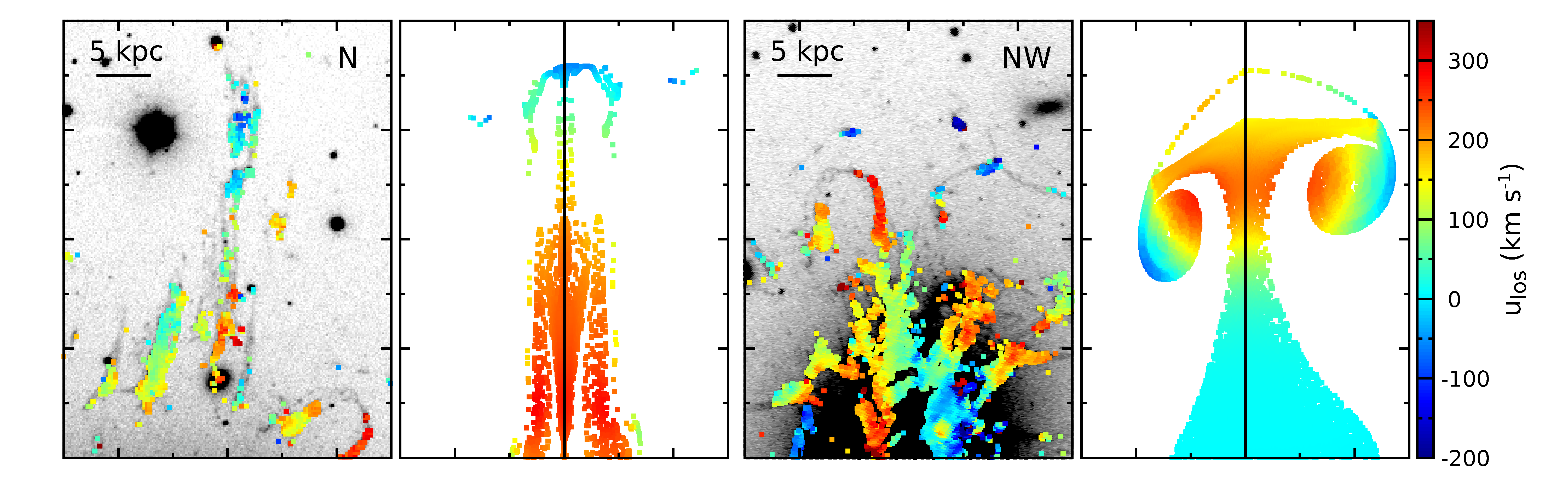
The velocity gradient revealed in the long northern filament (the first panel in Fig. 13) is well captured in our model. It can be explained by a stretching process taking place when eddies detach from the bubble (see Fig. 7). In the residual X-ray image (Fig. 1), we tentatively find a bubble candidate to the north of the filament (marked by the arrow at the top), in line with the expectation of our scenario. If confirmed, it will be a detection of a bubble that has maintained its integrity while rising up to away from the cluster center. The bubble has also survived crossing cold fronts formed by a merger-induced gas sloshing (ZuHone et al. 2021, cf.). At the same time, our model produces the horseshoe-shaped filaments, which trace the streamlines downstream of the bubble (Fabian et al. 2003). The “best-fit” LOS inclination angle in our model supports the scenario discussed in Section 4.1 that the northwestern bubble in Perseus moves slightly away from the plane of the sky.
Li et al. 2020 measured the first-order velocity structure function of the LOS velocity of H filaments in nearby clusters to probe turbulence in the ICM. Here, we carry out a similar exercise for our simulated bubble-driven gas velocity fields. Although small-scale turbulence could not be captured in 2D, our model sheds light on how the “bulk” (laminar) motions of the gas within the filaments and large eddies driven by intact bubbles contribute to the velocity structure function, as well as explore the effects of overlapping filaments and their spatial distribution on large scales. For this purpose, we generate a mock distribution of the filaments in 3D. We randomly select snapshots spanning from to with replacement in the simulation E4L12S. From each snapshot, we extract one filament constructed from the particles initially located within (at ) but within the shell at the present time and assume that the filament resides only in one plane (e.g., the cross section between the ring-shaped particles and the plane). We then set random orientations for these filaments and assemble them together to form a 2D projected distribution. We assume simply that those filaments do not interfere with each other, though the situation could, of course, be more complicated in reality. The top panels of Fig. 14 show two realizations of our mock distributions with . The color encodes the filament LOS velocities . These examples have morphologies that are similar to real observations (see, e.g., Fig. 1). We then calculate the first-order structure function of the velocity as
| (6) |
where , and denotes the operator of averaging over all velocity pairs.
The bottom panel of Fig. 14 shows our structure functions averaged over realizations. The error bars indicate the standard deviation. The curves with and are very similar except for the scatter. Our model shows that, in general, the structure function increases with approximately as on small scales () and gradually becomes flat when . The transition is smooth and its characteristic scale () is comparable to the bubble size. Qualitatively, one could explain the shape of our in the following way. Due to the sparse distribution of the filaments, the structure function is dominated by the velocity pairs across two separate filaments on large scales. If motions of the gas that forms a filament are mostly driven by a bubble, there will be no significant correlation between the filaments. That is exactly the case in our model by design. It explains why the curve tends to be flat in the large-scale regime and why the error bars shrink significantly at when we increase from to . In contrast, on small scales, the structure function is largely determined by the velocity gradients in individual filaments. For the simplest case of a uniformly stretched straight filament, we would have . The structure function’s amplitude (but not its shape) depends on the angle between the filament and LOS as well, causing a scatter in the structure function. Meanwhile, substructures in individual filaments, eddies, and overlapping of multiple filaments all complicate the filament distribution on small scales and make the overall slope of the structure function shallower than unity. We can clearly see such complexities in the top panels of Fig. 14. Note that, in our scenario, there is no guarantee that the shape of should be a power law. We have also estimated the structure function for the simulation E4L24 (different bubble size and particle sampling strategy) and found a similar result as in Fig. 14.
The structure function in Fig. 14 is surprisingly consistent with the observations by Li et al. 2020 in both amplitude and shape, especially given that no parameter is fine-tuned in our model. This result reveals an alternative interpretation for these observations, namely that, the structure function is dominated by the characteristic velocity pattern and spatial structure of the gas driven by intact bubbles in the cluster core rather than by well-developed turbulence, as proposed in Li et al. 2020. We also note that, even though there is no 3D turbulence in our simulations, the gas velocity in the bubble wake (e.g., eddies, reverse jet) is to times higher than the bubble-rise velocity (see Fig. 8), much stronger than the turbulent motions () measured with Hitomi in Perseus (Hitomi Collaboration 2018). The filament velocities should therefore always be dominated by the bubble-driven “bulk” motions rather than by turbulence. A remarkable consistency between our model and H observations of the gas velocity distribution in filaments suggests that even though small-scale turbulence is likely developed in reality, it may not affect the gas velocity field strongly, at least not on the scale of the bubble.

Since the slope of our structure function is steeper than the prediction for the turbulence in the classical Kolmogorov scenario (), it is possible that, on sufficiently small scales, turbulence becomes dominant. It is thus interesting to ask if estimating the velocity structure function for H filaments is a robust way to detect turbulence properties on those scales. How do projection effects and sparsity of the filaments’ distribution affect the measurements? We shed some light on these questions by performing a simple experiment based on our simulations. We generate Gaussian random velocity fields with an underlying energy spectrum
| (7) |
where is a normalization constant setting the standard deviation of the velocity field as , is the spectral index, is the cutoff wavenumber fixed at a scale larger than our system. Note that, we are only interested in the small scale () in this experiment. In reality, the characteristic should be related with the specific driving mechanisms of the turbulence. The shape of small- spectral tail might be also shallower (see, e.g., Hosking & Schekochihin 2022).
We repeat our procedure of generating filaments in 3D, projecting them and calculating the structure function (Fig. 14), but we replace the LOS velocity of the filaments with the Gaussian random field.1010 10 The new filament velocity is proximally interpolated from the data cube of the Gaussian random field, whose spatial resolution is . For comparison, we also calculate the 3D structure function based on the full spatial information of the filaments rather than the projected one. The results are shown in Fig. 15, where we examine two different energy spectra with (Kolmogorov type) and . The solid black lines show the baseline results directly estimated from the 3D data cube of the velocity field. Our 3D (the red lines) recovers the input accurately for both spectra. The sparsity of the filaments does not have any effect on the measurement. The 2D , however, obviously biases the curves due to projection effects (Li et al. 2020). It infers a shallower energy spectrum in the inertial range compared to the baseline model. However, careful modeling (e.g., as done in Fig. 15) might be used to correct this bias. We conclude that measuring structure functions of the embedded cold gas may still be a robust approach to detect turbulence in the ICM, as long as (1) the cold and hot gas phases are tightly coupled together and (2) the gas velocity is dominated by turbulent motion.
5 Conclusions
In this study, we start with an assumption that buoyant bubbles in cluster cores maintain their shapes during their rise. We model them as cap-shaped bodies and show the important role of such “rigid” bubbles and their long-term interactions with the ambient ICM in shaping the gas velocity distribution and forming thin gaseous structures (e.g., H filaments) in cluster cores.
In our rigid-bubble simulations, in the wakes of buoyantly rising bubbles, eddies are formed with a size comparable to the bubble. The morphology of their streamlines is similar to the horseshoe-shaped H filaments observed in the Perseus cluster, supporting the scenario proposed by Fabian et al. 2003. We find that most of the gas mass uplifted by bubbles is through “eddy transport” rather than Darwin drift, i.e., the gas is trapped inside the downstream eddies and moves together with the rising bubble. The evolution of the eddies is significantly affected by the gravitational field during the rise, characterized by the bubble’s Froude number . The eddies are gradually elongated along the bubble’s direction of movement and eventually detach from the bubble. In this process, the stretched eddies quickly evolve into a high-speed reverse jet-like stream propagating towards (and possibly even shooting through) the cluster center in our model. The typical gas velocity in the bubble wake is higher than the bubble-rise velocity, e.g., by a factor of in the eddies and in the jet, showing only weak dependence on Fr (see Fig. 8). The jet structure provides a natural explanation for the long cold gas filaments observed in nearby clusters (e.g., Perseus; see Fig. 1).
We make a detailed comparison of our model with the observations of the Perseus cluster using both the X-ray-weighted gas velocity dispersion (Hitomi Collaboration 2018) and LOS velocities of H filaments (Gendron-Marsolais et al. 2018). Using our simulations, we predict the terminal velocity of the northwestern bubble in Perseus (; see also 72) and find that an inclination angle of the LOS is required to explain the velocity dispersion excess () observed downstream of the bubble by Hitomi (see Fig. 11). If the bubble moved in the plane of the sky, the observed peak velocity dispersion would be times smaller than the bubble-rise velocity, due to the fact that the bubble size is smaller than the scale of the cluster’s gas core.
Under the assumption that the cold and hot gas phases efficiently couple dynamically, our simulations illustrate the formation of both the long straight H filament and the horseshoe-shaped filament in Perseus. The model matches well the observed filament morphology, spatial extent, and the LOS velocity distribution (see Fig. 13). To complement this morphological study, we assemble mock distributions of the filaments in 3D to estimate their projected LOS velocity structure function as done in Li et al. 2020. Without fine-tuning of any parameters, our model reproduces both the observed structure function’s amplitude and shape (see Fig. 14), revealing a simple interpretation for the observational measurements – the structure function of the filaments is dominated by velocity gradients of inward and outward laminar gas flows and large eddies formed behind the bubbles. The uniform, small-scale turbulence, if present, cannot be probed through the structure function of H filaments because the “bulk” velocity pattern is dominant. Overlapping of filaments on small scales and their sparse distribution on large scales also affect the shape of the structure function at small and large separations, respectively.
Finally, we acknowledge the major simplification made in this study. Given the 2.5D rigid-bubble model adopted by us, (1) bubble deformation during the rise, (2) small-scale 3D turbulence, and (3) rapid inflation of the bubbles in the early phase of the AGN feedback (i.e., bubble-jet interaction) are not captured. Gas cooling is also neglected along with ambient gas flows driven by sloshing. Determining how these processes affect our results quantitatively needs a more detailed investigation in the future. Nevertheless, our model appears to capture several key features of the gas velocity distribution driven by intact rising bubbles in the cluster cores and may help interpret current and future observations (from, e.g., XRISM, Athena).
Acknowledgments
Support for this work was provided by the National Aeronautics and Space Administration through Chandra Award Number TM1-22008X issued by the Chandra X-ray Center, which is operated by the Smithsonian Astrophysical Observatory for and on behalf of the National Aeronautics Space Administration under contract NAS8-03060. Part of the simulations presented in this paper were carried out using the Midway computing cluster provided by the University of Chicago Research Computing Center. IZ is partially supported by a Clare Boothe Luce Professorship from the Henry Luce Foundation. The work of AAS was supported in part by UK EPSRC grant EP/R034737/1. WF acknowledges support from the Smithsonian Institution, the Chandra High Resolution Camera Project through NASA contract NAS8-03060, and NASA Grants 80NSSC19K0116, GO1-22132X, and GO9-20109X.
Data Availability
The data underlying this article will be shared on reasonable request to the corresponding author.

References
- Agertz et al. (2007) Agertz O., Moore B., Stadel J., Potter D., Miniati F., Read J., Mayer L., et al., 2007, MNRAS, 380, 963
- Bauer & Springel (2012) Bauer A., Springel V., 2012, MNRAS, 423, 2558
- Bhaga & Weber (1981) Bhaga D., Weber M. E., 1981, JFM, 105, 61
- Brüggen, Scannapieco, & Heinz (2009) Brüggen M., Scannapieco E., Heinz S., 2009, MNRAS, 395, 2210
- Bîrzan et al. (2004) Bîrzan L., Rafferty D. A., McNamara B. R., Wise M. W., Nulsen P. E. J., 2004, ApJ, 607, 800
- Braginskii (1958) Braginskii, S. I. 1958, Soviet Journal of Experimental and Theoretical Physics, 6, 358
- Brienza et al. (2021) Brienza M., Shimwell T. W., de Gasperin F., Bikmaev I., Bonafede A., Botteon A., Brüggen M., et al., 2021, NatAs, 5, 1261
- Candelaresi & Del Sordo (2020) Candelaresi S., Del Sordo F., 2020, ApJ, 896, 86
- Churazov et al. (2000) Churazov E., Forman W., Jones C., Böhringer H., 2000, A&A, 356, 788
- Churazov et al. (2001) Churazov E., Brüggen M., Kaiser C. R., Böhringer H., Forman W., 2001, ApJ, 554, 261
- Churazov et al. (2002) Churazov E., Sunyaev R., Forman W., Böhringer H., 2002, MNRAS, 332, 729
- Churazov et al. (2003) Churazov E., Forman W., Jones C., Böhringer H., 2003, ApJ, 590, 225
- Conselice, Gallagher, & Wyse (2001) Conselice C. J., Gallagher J. S., Wyse R. F. G., 2001, AJ, 122, 2281
- Darwin (1953) Darwin C., 1953, PCPS, 49, 342
- Diehl et al. (2008) Diehl S., Li H., Fryer C. L., Rafferty D., 2008, ApJ, 687, 173
- Duan & Guo (2018) Duan X., Guo F., 2018, ApJ, 861, 106
- Fabian et al. (2003) Fabian A. C., Sanders J. S., Crawford C. S., Conselice C. J., Gallagher J. S., Wyse R. F. G., 2003, MNRAS, 344, L48
- Fabian et al. (2006) Fabian A. C., Sanders J. S., Taylor G. B., Allen S. W., Crawford C. S., Johnstone R. M., Iwasawa K., 2006, MNRAS, 366, 417
- Fabian (2012) Fabian A. C., 2012, ARA&A, 50, 455
- Forman et al. (2007) Forman W., Jones C., Churazov E., Markevitch M., Nulsen P., Vikhlinin A., Begelman M., et al., 2007, ApJ, 665, 1057
- Fornberg (1988) Fornberg B., 1988, JFM, 190, 471
- Gaspari, Ruszkowski, & Sharma (2012) Gaspari M., Ruszkowski M., Sharma P., 2012, ApJ, 746, 94
- Gendron-Marsolais et al. (2018) Gendron-Marsolais M., Hlavacek-Larrondo J., Martin T. B., Drissen L., McDonald M., Fabian A. C., Edge A. C., et al., 2018, MNRAS, 479, L28
- Gull & Northover (1973) Gull S. F., Northover K. J. E., 1973, Natur, 244, 80
- Hitomi Collaboration (2018) Hitomi Collaboration, 2018, PASJ, 70, 9
- Hlavacek-Larrondo et al. (2012) Hlavacek-Larrondo J., Fabian A. C., Edge A. C., Ebeling H., Sanders J. S., Hogan M. T., Taylor G. B., 2012, MNRAS, 421, 1360
- Hosking & Schekochihin (2022) Hosking D. N., Schekochihin A. A., 2022, arXiv:2202.00462
- Hu et al. (2022) Hu H., Qiu Y., Gendron-Marsolais M.-L., Bogdanović T., Hlavacek-Larrondo J., Ho L. C., Inayoshi K., et al., 2022, ApJL, 929, L30
- Ichinohe et al. (2017) Ichinohe Y., Simionescu A., Werner N., Takahashi T., 2017, MNRAS, 467, 3662
- Kaiser et al. (2005) Kaiser C. R., Pavlovski G., Pope E. C. D., Fangohr H., 2005, MNRAS, 359, 493
- Lee (2000) Lee S., 2000, Computers & Fluids, 29, 639
- Li & Bryan (2014) Li Y., Bryan G. L., 2014, ApJ, 789, 54
- Li et al. (2020) Li Y., Gendron-Marsolais M.-L., Zhuravleva I., Xu S., Simionescu A., Tremblay G. R., Lochhaas C., et al., 2020, ApJL, 889, L1
- Lighthill (1956) Lighthill M. J., 1956, JFM, 1, 31
- Magnaudet & Mercier (2020) Magnaudet J., Mercier M. J., 2020, AnRFM, 52, 61
- McDonald et al. (2010) McDonald M., Veilleux S., Rupke D. S. N., Mushotzky R., 2010, ApJ, 721, 1262
- McDonald, Veilleux, & Rupke (2012) McDonald M., Veilleux S., Rupke D. S. N., 2012, ApJ, 746, 153
- McNamara et al. (2000) McNamara B. R., Wise M., Nulsen P. E. J., David L. P., Sarazin C. L., Bautz M., Markevitch M., et al., 2000, ApJL, 534, L135
- McNamara & Nulsen (2007) McNamara B. R., Nulsen P. E. J., 2007, ARA&A, 45, 117
- McNamara et al. (2016) McNamara B. R., Russell H. R., Nulsen P. E. J., Hogan M. T., Fabian A. C., Pulido F., Edge A. C., 2016, ApJ, 830, 79
- Mohapatra et al. (2022) Mohapatra R., Jetti M., Sharma P., Federrath C., 2022, MNRAS, 510, 2327
- Nakamura (1996) Nakamura Y., 1996, Journal of Fluids and Structures 10, 159
- Okino et al. (2021) Okino S., Akiyama S., Takagi K., Hanazaki H., 2021, JFM, 927, A15
- Olivares et al. (2019) Olivares V., Salome P., Combes F., Hamer S., Guillard P., Lehnert M. D., Polles F. L., et al., 2019, A&A, 631, A22
- Pope et al. (2010) Pope E. C. D., Babul A., Pavlovski G., Bower R. G., Dotter A., 2010, MNRAS, 406, 2023
- Qiu et al. (2020) Qiu Y., Bogdanović T., Li Y., McDonald M., McNamara B. R., 2020, NatAs, 4, 900
- Qiu et al. (2021) Qiu Y., Hu H., Inayoshi K., Ho L. C., Bogdanović T., McNamara B. R., 2021, ApJL, 917, L7
- Randall et al. (2015) Randall S. W., Nulsen P. E. J., Jones C., Forman W. R., Bulbul E., Clarke T. E., Kraft R., et al., 2015, ApJ, 805, 112
- Revaz, Combes, & Salomé (2008) Revaz Y., Combes F., Salomé P., 2008, A&A, 477, L33
- Reynolds et al. (2005) Reynolds C. S., McKernan B., Fabian A. C., Stone J. M., Vernaleo J. C., 2005, MNRAS, 357, 242
- Reynolds, Balbus, & Schekochihin (2015) Reynolds C. S., Balbus S. A., Schekochihin A. A., 2015, ApJ, 815, 41
- Roediger et al. (2013) Roediger E., Kraft R. P., Forman W. R., Nulsen P. E. J., Churazov E., 2013, ApJ, 764, 60
- Russell et al. (2019) Russell H. R., McNamara B. R., Fabian A. C., Nulsen P. E. J., Combes F., Edge A. C., Madar M., et al., 2019, MNRAS, 490, 3025
- Ruszkowski et al. (2007) Ruszkowski M., Enßlin T. A., Brüggen M., Heinz S., Pfrommer C., 2007, MNRAS, 378, 662
- Sanders et al. (2016) Sanders J. S., Fabian A. C., Taylor G. B., Russell H. R., Blundell K. M., Canning R. E. A., Hlavacek-Larrondo J., et al., 2016, MNRAS, 457, 82
- Sakamoto & Haniu (1990) Sakamoto H., Haniu H., 1990, Journal of Fluids Engineering-Transactions of The Asme, 112, 386
- Scannapieco & Brüggen (2008) Scannapieco E., Brüggen M., 2008, ApJ, 686, 927
- Schiller & Naumann (1935) Schiller L., Naumann Z., 1935, VDI Zeitung, 77, 318
- Sharma et al. (2012) Sharma P., McCourt M., Quataert E., Parrish I. J., 2012, MNRAS, 420, 3174
- Spitzer (1962) Spitzer L., 1962, Physics of Fully Ionized Gases, 2nd edn. Interscience. New York
- Torres et al. (2000) Torres C. R., Hanazaki H., Ochoa J., Castillo J., van Woert M., 2000, JFM, 417, 211
- Tremblay et al. (2012) Tremblay G. R., O’Dea C. P., Baum S. A., Clarke T. E., Sarazin C. L., Bregman J. N., Combes F., et al., 2012, MNRAS, 424, 1026
- Tripathi, Sahu, & Govindarajan (2015) Tripathi M. K., Sahu K. C., Govindarajan R., 2015, NatCo, 6, 6268
- Wadsley, Veeravalli, & Couchman (2008) Wadsley J. W., Veeravalli G., Couchman H. M. P., 2008, MNRAS, 387, 427
- Walker et al. (2017) Walker S. A., Hlavacek-Larrondo J., Gendron-Marsolais M., Fabian A. C., Intema H., Sanders J. S., Bamford J. T., et al., 2017, MNRAS, 468, 2506
- Wang & Markevitch (2018) Wang Q. H. S., Markevitch M., 2018, ApJ, 868, 45
- Wang et al. (2021) Wang C., Ruszkowski M., Pfrommer C., Oh S. P., Yang H.-Y. K., 2021, MNRAS, 504, 898
- Werner et al. (2013) Werner N., Oonk J. B. R., Canning R. E. A., Allen S. W., Simionescu A., Kos J., van Weeren R. J., et al., 2013, ApJ, 767, 153
- Werner et al. (2019) Werner, N., McNamara, B. R., Churazov, E., et al. 2019, Space Sci. Rev., 215, 5
- Wise et al. (2007) Wise M. W., McNamara B. R., Nulsen P. E. J., Houck J. C., David L. P., 2007, ApJ, 659, 1153
- XRISM Science Team (2020) XRISM Science Team, 2020, arXiv:2003.04962
- Zhang, Churazov, & Schekochihin (2018) Zhang C., Churazov E., Schekochihin A. A., 2018, MNRAS, 478, 4785
- Zhuravleva et al. (2015) Zhuravleva I., Churazov E., Arévalo P., Schekochihin A. A., Allen S. W., Fabian A. C., Forman W. R., et al., 2015, MNRAS, 450, 4184
- Zhuravleva et al. (2019) Zhuravleva I., Churazov E., Schekochihin A. A., Allen S. W., Vikhlinin A., Werner N., 2019, NatAs, 3, 832
- ZuHone et al. (2021) ZuHone J. A., Markevitch M., Weinberger R., Nulsen P., Ehlert K., 2021, ApJ, 914, 73
Appendix A Resolution test
To test how our simulation results depend on the effective spatial resolution, we rerun the simulation E4L12 with two different resolutions, and , i.e., lower and higher than the default value by a factor of 2. The comparisons of gas velocities and distributions of tracer particles are shown in Fig. 16 (see also Fig. 4). The runs with different resolutions show similar results, including the evolution of bubble velocity pattern, formation of eddies, the moment of the eddy detachment, and the formation of a reverse jet. It demonstrates that our findings are not affected by the resolution. Despite, there are minor differences between the low and high-resolution runs. The high-resolution results show stronger gas velocities in the eddies and reverse jet by per cent and also more prominent instabilities formed near the tip of the reverse jet. These differences are in line with the expectations – simulations with higher resolution capture more instabilities and turbulent gas structures. These, however, do not affect the velocity structure function modeled in Section 4.2.