RankSeg: Adaptive Pixel Classification with Image Category Ranking for Segmentation
Abstract
The segmentation task has traditionally been formulated as a complete-label11 1 We use the term “complete label” to represent the set of all predefined categories in the dataset. pixel classification task to predict a class for each pixel from a fixed number of predefined semantic categories shared by all images or videos. Yet, following this formulation, standard architectures will inevitably encounter various challenges under more realistic settings where the scope of categories scales up (e.g., beyond the level of ). On the other hand, in a typical image or video, only a few categories, i.e., a small subset of the complete label are present. Motivated by this intuition, in this paper, we propose to decompose segmentation into two sub-problems: (i) image-level or video-level multi-label classification and (ii) pixel-level rank-adaptive selected-label classification. Given an input image or video, our framework first conducts multi-label classification over the complete label, then sorts the complete label and selects a small subset according to their class confidence scores. We then use a rank-adaptive pixel classifier to perform the pixel-wise classification over only the selected labels, which uses a set of rank-oriented learnable temperature parameters to adjust the pixel classifications scores. Our approach is conceptually general and can be used to improve various existing segmentation frameworks by simply using a lightweight multi-label classification head and rank-adaptive pixel classifier. We demonstrate the effectiveness of our framework with competitive experimental results across four tasks, including image semantic segmentation, image panoptic segmentation, video instance segmentation, and video semantic segmentation. Especially, with our RankSeg, MaskFormer gains +/+/+ on ADEK panoptic segmentation/YouTubeVIS video instance segmentation/VSPW video semantic segmentation benchmarks respectively. Code is available at: {https://github.com/openseg-group/RankSeg}
Keywords:
Rank-Adaptive, Selected-Label, Image Semantic Segmentation, Image Panoptic Segmentation, Video Instance Segmentation, Video Semantic Segmentation1 Introduction


Image and video segmentation, i.e., partitioning images or video frames into multiple meaningful segments, is a fundamental computer vision research topic that has wide applications including autonomous driving, surveillance system, and augmented reality. Most recent efforts have followed the path of fully convolutional networks [56] and proposed various advanced improvements, e.g., high-resolution representation learning [62, 72], contextual representation aggregation [12, 23, 35, 89, 83], boundary refinement [68, 44, 86], and vision transformer architecture designs [55, 63, 84, 90].
Most of the existing studies formulate the image and video segmentation problem as a complete-label pixel classification task. In the following discussion, we’ll take image semantic segmentation as an example for convenience. For example, image semantic segmentation needs to select the label of each pixel from the complete label22 2 We use “label”, “category”, and “class” interchangeably. set that is predefined in advance. However, it is unnecessary to consider the complete label set for every pixel in each image as most standard images only consist of objects belonging to a few categories. Figure 3 plots the statistics on the percentage of images that contain no more than the given class number in the entire dataset vs. the number of classes that appear within each image. Accordingly, we can see that , , , and of images contain less than categories on PASCAL-Context [59], COCO-Stuff [8], ADEK-Full [19, 91], and COCO+LVIS [29, 40] while each of them contains , , , and predefined semantic categories respectively. Besides, Figure 1 shows an example image that only contains classes while the complete label set consists of predefined categories.
To take advantage of the above observations, we propose to re-formulate the segmentation task into two sub-problems including multi-label image/video classification and rank-adaptive pixel classification over a subset of selected labels. To verify the potential benefits of our method, we investigate the gains via exploiting the ground-truth multi-label of each image or video. In other words, the pixel classifier only needs to select the category of each pixel from a collection of categories presented in the current image or video, therefore, we can filter out all other categories that do not appear. Figure 3 summarizes the comparison results based on Segmenter [67] and MaskFormer [18]. We can see that the segmentation performance is significantly improved given the ground-truth multi-label prediction. In summary, multi-label classification is an important but long-neglected sub-problem on the path toward more accurate segmentation.
Motivated by the significant gains obtained with the ground-truth multi-label, we propose two different schemes to exploit the benefit of multi-label image predictions including the independent single-task scheme and joint multi-task scheme. For the independent single-task scheme, we train one model for multi-label image/video classification and another model for segmentation. Specifically, we first train a model to predict multi-label classification probabilities for each image/video, then we estimate the existing label subset for each image/video based on the multi-label predictions, last we use the predicted label subset to train the segmentation model for rank-adaptive selected-label pixel classification during both training and testing. For the joint multi-task scheme, we train one model to support both multi-label image/video classification and segmentation based on a shared backbone. Specifically, we apply a multi-label prediction head and a segmentation head, equipped with a rank-adaptive adjustment scheme, over the shared backbone and train them jointly. For both schemes, we need to send the multi-label predictions into the segmentation head for rank-adaptive selected-label pixel classification, which enables selecting a collection of categories that appear and adjusting the pixel-level classification scores according to the image/video content adaptively.
We demonstrate the effectiveness of our approach on various strong baseline methods including DeepLabv [12], Segmenter [67], Swin-Transformer [55], BEiT [4], MaskFormer [19], MaskFormer [18], and ViT-Adapter [15] across multiple segmentation benchmarks including PASCAL-Context [59], ADEK [91], COCO-Stuff [8], ADEK-Full [91, 19], COCO+LVIS [29, 40], YouTubeVIS [80], and VSPW [58].
2 Related Work
Image segmentation. We can roughly categorize the existing studies on image semantic segmentation into two main paths: (i) region-wise classification methods [1, 7, 27, 26, 76, 60, 7, 69], which first organize the pixels into a set of regions (usually super-pixels), and then classify each region to get the image segmentation result. Several very recent methods [19, 88, 71] exploit the DETR framework [10] to conduct region-wise classification more effectively; (ii) pixel-wise classification methods, which predict the label of each pixel directly and dominate most previous studies since the pioneering FCN [56]. There exist extensive follow-up studies that improve the pixel classification performance via constructing better contextual representations [89, 12, 85, 83] or designing more effective decoder architectures [3, 66, 13]. Image panoptic segmentation [43, 42] aims to unify image semantic segmentation and image instance segmentation tasks. Some recent efforts have introduced various advanced architectures such as Panoptic FPN [42], Panoptic DeepLab [17], Panoptic Segformer [49], K-Net [88], and MaskFormer [18]. Our RankSeg is complementary with various paradigms and consistently improves several representative state-of-the-art methods across both image semantic segmentation and image panoptic segmentation tasks.
Video segmentation. Most of the previous works address the video segmentation task by extending the existing image segmentation models with temporal consistency constraint [73]. Video semantic segmentation aims to predict the semantic category of all pixels in each frame of a video sequence, where the main efforts focus on two paths including exploiting cross-frame relations to improve the prediction accuracy [45, 36, 41, 25, 61, 11] and leveraging the information of neighboring frames to accelerate computation [57, 79, 48, 39, 34, 54]. Video instance segmentation [80] requires simultaneous detection, segmentation and tracking of instances in videos and there exist four mainstream frameworks including tracking-by-detection [70, 50, 9, 24, 32], clip-and-match [6, 2], propose-and-reduce [51], and segment-as-a-whole [74, 37, 77, 16]. We show the effectiveness of our method on both video semantic segmentation and video instance segmentation tasks via improving the very recent state-of-the-art method MaskFormer [16].
Multi-label classification. The goal of multi-label classification is to identity all the categories presented in a given image or video over the complete label set. The conventional multi-label image classification literature partitions the existing methods into three main directions: (i) improving the multi-label classification loss functions to handle the imbalance issue [78, 5], (ii) exploiting the label co-occurrence (or correlations) to model the semantic relationships between different categories [33, 47, 14, 81], and (iii) localizing the diverse image regions associated with different categories [75, 28, 82, 46, 53]. In our independent single-task scheme, we choose the very recent state-of-the-art method Query2Label [53] to perform multi-label classification on various semantic segmentation benchmarks as it is a very simple and effective method that exploits the benefits of both label co-occurrence and localizing category-dependent regions. There exist few efforts that apply multi-label image classification to address segmentation task. To the best of our knowledge, the most related study EncNet [87] simply adds a multi-label image classification loss w/o changing the original semantic segmentation head that still needs to select the label of each pixel from all predefined categories. We empirically show the advantage of our method over EncNet in the ablation experiments. Besides, our proposed method is naturally suitable to solve large-scale semantic segmentation problem as we only perform rank-adaptive pixel classification over a small subset of the complete label set based on the multi-label image prediction. We also empirically verify the advantage of our method over the very recent ESSNet [40] in the ablation experiments.
3 Our Approach
We first introduce the overall framework of our approach in Sec. 3.1, which is also illustrated in Figure 4. Second, we introduce the details of the independent single-task scheme in Sec. 3.2 and those of joint multi-task scheme in Sec. 3.3. Last, we conduct analysis experiments to investigate the detailed improvements of our method across multiple segmentation tasks in Sec. 3.4.
3.1 Framework
The overall framework of our method is illustrated in Figure 4, which consists of one path for multi-label image classification and one path for semantic segmentation. The multi-label prediction is used to sort and select the top category embeddings with the highest confidence scores which are then sent into the rank-adaptive selected-label pixel classifier to generate the semantic segmentation prediction. We explain the mathematical formulations of both multi-label image classification and rank-adaptive selected-label pixel classification as follows:
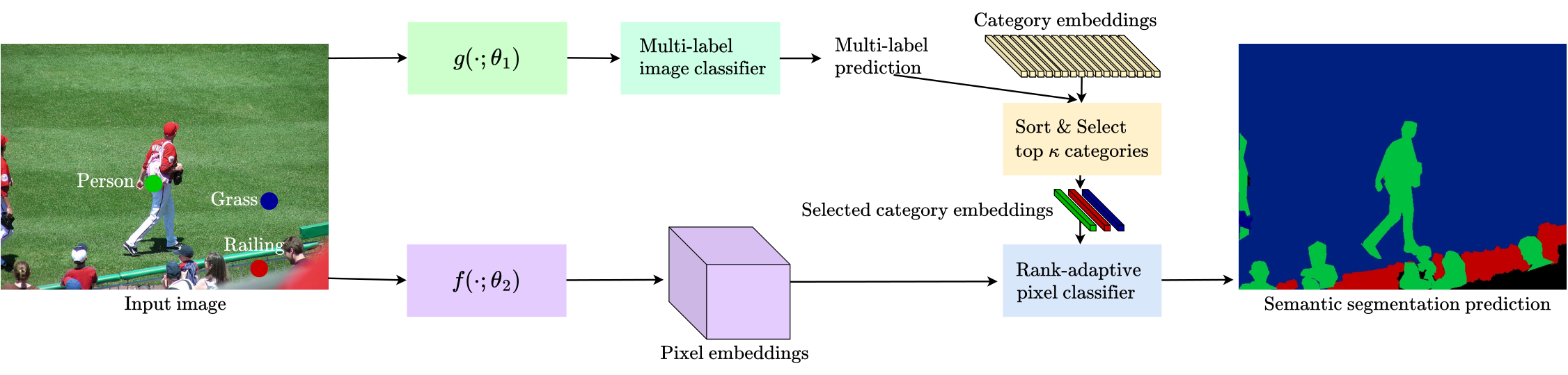
Multi-label image classification. The goal of multi-label image classification is to predict the set of existing labels in a given image , where and represent the input height and width. We generate the image-level multi-label ground truth from the ground truth segmentation map and we represent with a vector of binary values , where represents the total number of predefined categories and represents the existence of pixels belonging to -th category and otherwise.
The prediction is a vector that records the existence confidence score of each category in the given image . We use to represent the backbone for the multi-label image classification model. We estimate the multi-label predictions of input with the following sigmoid function:
| (1) |
where is the -th element of , represents the output feature map, represents the multi-label image classification weight associated with the -th category, and represents a transformation function that estimates the similarity between the output feature map and the multi-label image classification weights. We supervise the multi-label predictions with the asymmetric loss that operates differently on positive and negative samples by following [5, 53].
Rank-adaptive selected-label pixel classification. The goal of semantic segmentation is to predict the semantic label of each pixel and the label is selected from all predefined categories. We use to represent the predicted pixel classification probability map for the input image . We use to represent the semantic segmentation backbone and to represent the ground-truth segmentation map. Instead of choosing the label of each pixel from all predefined categories, based on the previous multi-label prediction for image , we introduce a more effective rank-adaptive selected-label pixel classification scheme:
- •
Sort and select the top elements of the classifier weights according to the descending order of multi-label predictions :
(2) - •
Rank-adaptive classification of pixel over the top selected categories:
(3)
where represents the pixel classification weights for all predefined categories and represents the top selected pixel classification weights associated with the largest multi-label classification scores. represents the output feature map for semantic segmentation. represents a transformation function that estimates the similarity between the pixel features and the pixel classification weights. represents the number of selected category embeddings and is chosen as a much smaller value than .
We apply a set of rank-adaptive learnable temperature parameters to adjust the classification scores over the selected top categories. The temperature parameters across different selected classes are shared in all of the baseline experiments by default33 3 We set === for all baseline segmentation experiments.. We analyze the influence of choices and the benefits of such a rank-oriented adjustment scheme in the following discussions and experiments.
3.2 Independent single-task scheme
Under the independent single-task setting, the multi-label image classification model and the semantic segmentation model are trained separately and their model parameters are not shared, i.e., . Specifically, we first train the multi-label image classification model to identify the top most likely categories for each image. Then we train the rank-adaptive selected-label pixel classification model, i.e., semantic segmentation model, to predict the label of each pixel over the selected top classes.
Multi-label image classification model. We choose the very recent SOTA multi-label classification method QueryLabel [53] as it performs best on multiple multi-label classification benchmarks by the time of our submission according to paper-with-code.44 4 https://paperswithcode.com/task/multi-label-classification The key idea of QueryLabel is to use the category embeddings as the query to gather the desired pixel embeddings as the key/value, which is output by an ImageNet-K pre-trained backbone such as Swin-L, adaptively with one or two transformer decoder layers. Then QueryLabel scheme applies a multi-label image classifier over the refined category embeddings to predict the existence of each category. Figure 5(a) illustrates the framework of QueryLabel framework. Refer to [53] and the official implementation for more details. The trained weights of QueryLabel model are fixed during both training and inference of the following semantic segmentation model.
Rank-adaptive selected-label pixel classification model. We choose a simple yet effective baseline Segmenter [67] as it achieves even better performance than Swin-L55 5 Segmenter w/ ViT-L: vs. Swin-L: on ADEK. when equipped with ViT-L. Segmenter first concatenates the category embedding with the pixel embeddings output by a ViT model together and then sends them into two transformer encoder layers. Last, based on the refined pixel embeddings and category embeddings, Segmenter computes their -normalized scalar product as the segmentation predictions. We select the top most likely categories for each image according to the predictions of the QueryLabel model and only use the selected top category embeddings instead of all category embeddings. Figure 5(b) illustrates the overall framework of Segmenter with the selected category embeddings.
3.3 Joint multi-task scheme
Considering that the independent single-task scheme suffers from extra heavy computation overhead as the QueryLabel method relies on a large backbone, e.g., Swin-L, we introduce a joint multi-task scheme that shares the backbone for both sub-tasks, in other words, and the computations of and are also shared.
Figure 6 shows the overall framework of the joint multi-task scheme. First, we apply a shared multi-task backbone to process the input image and output the pixel embeddings. Second, we concatenate the category embeddings with the down-sampled pixel embeddings66 6 Different from the semantic segmentation task, the multi-label image classification task does not require high-resolution representations., send them into one transformer encoder layer, and apply the multi-label image classifier on the refined category embeddings to estimate the multi-label predictions. Last, we sort and select the top category embeddings, concatenate the selected category embeddings with the pixel embeddings, send them into two transformer encoder layers, and compute the semantic segmentation predictions based on -normalized scalar product between the refined selected category embeddings and the refined pixel embeddings. We empirically verify the advantage of the joint multi-task scheme over the independent single-task scheme in the ablation experiments.
3.4 Analysis experiments
Oracle experiments. We first conduct several groups of oracle experiments based on Segmenter w/ ViT-B/ on four challenging image semantic segmentation benchmarks ( PASCAL-Context/COCO-Stuff/ADEK-Full/COCO+LVIS), MaskFormer w/ Swin-L on both ADEK panoptic segmentation benchmark77 7 We choose Swin-L by following the MODEL_ZOO of the official MaskFormer implementation: https://github.com/facebookresearch/Mask2Former and VSPW video semantic segmentation benchmark.
- Segmenter/MaskFormer + GT (train + eval): the upper-bound segmentation performance of Segmenter/MaskFormer when training & evaluating equipped with the ground-truth multi-label of each image or video, in other words, we only need to select the category of each pixel over the ground-truth existing categories in a given image or video.
- Segmenter/MaskFormer + GT (eval): the upper-bound segmentation performance of Segmenter/MaskFormer when only using the ground-truth multi-label of each image or video during evaluation.
Figure 3 illustrates the detailed comparison results. We can see that only applying the ground-truth multi-label during evaluation already brings considerable improvements and further applying the ground-truth multi-label during training significantly improves the segmentation performance across all benchmarks. For example, when compared to the baseline Segmenter or MaskFormer, Segmenter + GT (train + eval) gains +/+/+/+ absolute mIoU scores across PASCAL-Context/COCO-Stuff/ADEK-Full/COCO+LVIS and MaskFormer + GT (train + eval) gains +/+ on ADEK/VSPW.
Improvement analysis of RankSeg. Table 1 reports the results with different combinations of the proposed components within our joint multi-task scheme. We can see that: (i) multi-task learning (MT) introduces the auxiliary multi-label image classification task and brings relatively minor gains on most benchmarks, (ii) combining MT with label sorting & selection (LS) achieves considerable gains, and (iii) applying the rank-adaptive- manner (shown in Equation 3) instead of shared- achieves better performance. We investigate the possible reasons by analyzing the value distribution of learned with the rank-adaptive- manner in Figure 7, which shows that the learned is capable of adjusting the pixel classification scores based on the order of multi-label classification scores. In summary, we choose “MT + LS + RA” scheme by default, which gains +/+/+/+/+/+ over the baseline methods across these six challenging segmentation benchmarks respectively.
| Image semantic seg. | Image panoptic seg. | Video semantic seg. | ||||
|---|---|---|---|---|---|---|
| Method. | PASCAL-Context | COCO-Stuff | ADEK-Full | COCO+LVIS | ADEK | VSPW |
| Baseline | ||||||
| + MT | ||||||
| + MT + LS | ||||||
| + MT + LS + RA | ||||||
4 Experiment
4.1 Implementation details
We illustrate the details of the datasets, including ADEK [91], ADEK-Full [91, 19], PASCAL-Context [59], COCO-Stuff [8], COCO+LVIS [29, 40], VSPW [58], and YouTubeVIS [80], in the supplementary material.
Multi-label image classification. For the independent single-task scheme, following the official implementation88 8 https://github.com/SlongLiu/query2labels of QueryLabel, we train multi-label image classification models, e.g., ResNet- [31], TResNetL [64], and Swin-L [55], for epochs using Adam solver with early stopping. Various advanced tricks such as cutout [22], RandAug [21] and EMA [30] are also used. For the joint multi-task scheme, we simply train the multi-label image classification models following the same settings as the segmentation models w/o using the above-advanced tricks that might influence the segmentation performance. We illustrate more details of the joint multi-task scheme in the supplementary material.
Segmentation. We adopt the same settings for both independent single-task scheme and joint multi-task scheme. For the segmentation experiments based on Segmenter [67], DeepLabv [12], Swin-Transformer [55], BEiT [4], and ViT-Adapter [15]. we follow the default training & testing settings of their reproduced version based on mmsegmentation [20]. For the segmentation experiments based on MaskFormer or MaskFormer, we follow their official implementation99 9 https://github.com/facebookresearch/Mask2Former.
Hyper-parameters. We set as , , , , and on PASCAL-Context, ADEK, COCO-Stuff, ADEK-Full, and COCO+LVIS respectively as they consist of a different number of semantic categories. We set their multi-label image classification loss weights as , , , , and . The segmentation loss weight is set as . We illustrate the hyper-parameter settings of experiments on MaskFormer [19] or MaskFormer [18] in the supplementary material.
Metrics. We report mean average precision (mAP) for multi-label image classification task, mean intersection over union (mIoU) for image/video semantic segmentation task, panoptic quality (PQ) for panoptic segmentation task, and mask average precision (AP) for instance segmentation task.
| Method | COCO-Stuff | COCO+LVIS | ||||||
|---|---|---|---|---|---|---|---|---|
| #params. | FLOPs | mIoU () | #params. | FLOPs | mIoU () | |||
| Indep. single-task. | M | G | + | M | G | + | ||
| Joint multi-task. | M | G | + | M | G | + | ||
| COCO-Stuff | COCO+LVIS | ||||||||||
|---|---|---|---|---|---|---|---|---|---|---|---|
| mIoU () | |||||||||||
| + | + | + | + | + | + | + | + | + | + | + | |
| multi-label cls. loss weight | ||||
|---|---|---|---|---|
| mAP () | ||||
| mIoU () | ||||
| + | + | + | + |
| Method | #params. | FLOPs | mAP | mIoU () | |
|---|---|---|---|---|---|
| GAP+Linear | M | G | + | ||
| TranDec | M | G | + | ||
| TranEnc | M | G | + |
4.2 Ablation experiments
We conduct all ablation experiments based on the Segmenter w/ ViT-B and report their single-scale evaluation results on COCO-Stuff test and COCO+LVIS test if not specified. The baseline with Segmenter w/ ViT-B achieves and mIoU on COCO-Stuff and COCO+LVIS, respectively.
Influence of the multi-label classification accuracy. We investigate the influence of multi-label classification accuracy on semantic segmentation tasks based on the independent single-task scheme. We train multiple Query2Label models based on different backbones, e.g., ResNet, TResNetL, and Swin-L. Then we train three Segmenter w/ ViT-B segmentation models based on their multi-label predictions independently. According to the results in Table 6, we can see that more accurate multi-label classification prediction brings more semantic segmentation performance gains and less accurate multi-label classification prediction even results in worse results than baseline.
Independent single-task scheme vs. Joint multi-task scheme. We compare the performance and model complexity of the independent single-task scheme (w/ Swin-L) and joint multi-task scheme in Table 6. To ensure fairness, we choose the # of labels in the selected label set, i.e., , as for both schemes, and the segmentation models are trained & tested under the same settings. According to the comparison results, we can see that joint multi-task scheme achieves better performance with fewer parameters and FLOPs. Thus, we choose the joint multi-task scheme in the following experiments for efficiency if not specified.
Influence of different top . We study the influence of the size of selected label set, i.e., , as shown in Table 6. According to the results, our method achieves the best performance on COCO-Stuff/COCO+LVIS when =/=, which achieves a better trade-off between precision and recall for multi-label predictions. Besides, we attempt to fix = during training and report the results when changing during evaluation on COCO-Stuff: =: /=: /=: /=: . Notably, we also report the results with =, in other words, we only sort the classifier weights, which also achieve considerable gains. Therefore, we can see that sorting the classes and rank-adaptive adjustment according to multi-label predictions are the key to the gains. In summary, our method consistently outperforms baseline with different values. We also attempt to use dynamic for different images during evaluation but observe no significant gains. More details are provided in the supplementary material.
Influence of the multi-label classification loss weight. We study the influence of the multi-label image classification loss weights with the joint multi-task scheme on COCO-Stuff and report the results in Table 6. We can see that setting the multi-label classification loss weight as achieves the best performance.
Influence of choice. Table 6 compares the results based on different multi-label prediction head architecture choices including “GAP+Linear” (applying global average pooling followed by linear projection), “ TranDec” (using two transformer decoder layers), and “ TranEnc” (using one transformer encoder layer) on COCO-Stuff. Both “ TranDec” and “ TranEnc” operate on feature maps with resolution of the input image. According to the results, we can see that “ TranEnc” achieves the best performance and we implement as one transformer encoder layer if not specified. We also attempt generating multi-label prediction (mAP=) from the semantic segmentation prediction directly but observe no performance gains, thus verifying the importance of relatively more accurate multi-label classification predictions.
4.3 State-of-the-art experiments
Image semantic segmentation. We apply our method to various state-of-the-art image semantic segmentation methods including DeepLabv, Seg-Mask-L/, Swin-Transformer, BEiT, and ViT-Adapter-L. Table 8 summarizes the detailed comparison results across three semantic segmentation benchmarks including ADEK, COCO-Stuff, and COCO+LVIS, where we evaluate the multi-scale segmentation results on ADEK/COCO-Stuff and single-scale segmentation results on COCO+LVIS (due to limited GPU memory) respectively. More details of how to apply our joint multi-task scheme to these methods are provided in the supplementary material. According to the results in Table 8, we can see that our RankSeg consistently improves DeepLabv, Seg-Mask-L/, Swin-Transformer, BEiT, and ViT-Adapter-L across three evaluated benchmarks. For example, with our RankSeg, BEiT gains on ADEK with slightly more parameters and GFLOPs.
| Method | ADEK | COCO-Stuff | COCO+LVIS | ||||||
| #params. | FLOPs | mIoU() | #params. | FLOPs | mIoU() | #params. | FLOPs | mIoU() | |
| DeepLabv | M | G | M | G | M | G | |||
| + RankSeg | M | G | M | G | M | G | |||
| Seg-Mask-L/ | M | G | M | G | M | G | |||
| + RankSeg | M | G | M | G | M | G | |||
| Swin-B | M | G | M | G | M | G | |||
| + RankSeg | M | G | M | G | M | G | |||
| BEiT | M | G | M | G | OOM | ||||
| + RankSeg | M | G | M | G | OOM | ||||
| ViT-Adapter-L | M | G | NA | NA | |||||
| + RankSeg | M | G | NA | NA | |||||
| OOM means out of memory error on G V100 GPUs. | |||||||||
| Method | Image semantic seg. | Image panoptic seg. | Video semantic seg. | Video instance seg. | ||||||||
|---|---|---|---|---|---|---|---|---|---|---|---|---|
| ADEK | ADEK | VSPW (T=) | YouTubeVIS (T=) | |||||||||
| #params. | FLOPs | mIoU() | #params. | FLOPs | PQ() | #params. | FLOPs | mIoU() | #params. | FLOPs | AP() | |
| MaskFormer [18] | M | G | M | G | M | G | M | G | ||||
| + RankSeg | M | G | M | G | M | G | M | G | ||||
| T= means each video clip is composed of frames during training/evaluation and we report the GFLOPs over frames. | ||||||||||||
Image panoptic segmentation & Video semantic segmentation & Video instance segmentation.
To verify the generalization ability of our method,
we extend RankSeg to “rank-adaptive selected-label region classification” and apply it to the very recent MaskFormer [18].
According to Table 8,
our RankSeg improves the image semantic segmentation/image panoptic segmentation/video semantic segmentation/video instance segmentation performance by +/+
/+/+ respectively with slightly more parameters and GFLOPs.
More details about the MaskFormer experiments and the results of combining MaskFormer with RankSeg are provided in the supplementary material.
5 Conclusion
This paper introduces a general and effective rank-oriented scheme that formulates the segmentation task into two sub-problems including multi-label classification and rank-adaptive selected-label pixel classification. We first verify the potential benefits of exploiting multi-label image/video classification to improve pixel classification. We then propose a simple joint multi-task scheme that is capable of improving various state-of-the-art segmentation methods across multiple benchmarks. We hope our initial attempt can inspire more efforts towards using a rank-oriented manner to solve the challenging segmentation problem with a large number of categories. Last, we want to point out that designing & exploiting more accurate multi-label image/video classification methods is a long-neglected but very important sub-problem towards more general and accurate segmentation.
References
- [1] Arbeláez, P., Hariharan, B., Gu, C., Gupta, S., Bourdev, L., Malik, J.: Semantic segmentation using regions and parts. In: CVPR (2012)
- [2] Athar, A., Mahadevan, S., Osep, A., Leal-Taixé, L., Leibe, B.: Stem-seg: Spatio-temporal embeddings for instance segmentation in videos. In: ECCV. pp. 158–177. Springer (2020)
- [3] Badrinarayanan, V., Kendall, A., Cipolla, R.: Segnet: A deep convolutional encoder-decoder architecture for image segmentation. PAMI (2017)
- [4] Bao, H., Dong, L., Wei, F.: Beit: Bert pre-training of image transformers. arXiv preprint arXiv:2106.08254 (2021)
- [5] Ben-Baruch, E., Ridnik, T., Zamir, N., Noy, A., Friedman, I., Protter, M., Zelnik-Manor, L.: Asymmetric loss for multi-label classification. arXiv preprint arXiv:2009.14119 (2020)
- [6] Bertasius, G., Torresani, L.: Classifying, segmenting, and tracking object instances in video with mask propagation. In: CVPR. pp. 9739–9748 (2020)
- [7] Caesar, H., Uijlings, J., Ferrari, V.: Region-based semantic segmentation with end-to-end training. In: ECCV (2016)
- [8] Caesar, H., Uijlings, J., Ferrari, V.: Coco-stuff: Thing and stuff classes in context. In: CVPR (2018)
- [9] Cao, J., Anwer, R.M., Cholakkal, H., Khan, F.S., Pang, Y., Shao, L.: Sipmask: Spatial information preservation for fast image and video instance segmentation. In: ECCV. pp. 1–18. Springer (2020)
- [10] Carion, N., Massa, F., Synnaeve, G., Usunier, N., Kirillov, A., Zagoruyko, S.: End-to-end object detection with transformers. In: ECCV. pp. 213–229. Springer (2020)
- [11] Chandra, S., Couprie, C., Kokkinos, I.: Deep spatio-temporal random fields for efficient video segmentation. In: CVPR. pp. 8915–8924 (2018)
- [12] Chen, L.C., Papandreou, G., Schroff, F., Adam, H.: Rethinking atrous convolution for semantic image segmentation. arXiv:1706.05587 (2017)
- [13] Chen, L.C., Zhu, Y., Papandreou, G., Schroff, F., Adam, H.: Encoder-decoder with atrous separable convolution for semantic image segmentation. In: ECCV (2018)
- [14] Chen, T., Xu, M., Hui, X., Wu, H., Lin, L.: Learning semantic-specific graph representation for multi-label image recognition. In: ICCV (2019)
- [15] Chen, Z., Duan, Y., Wang, W., He, J., Lu, T., Dai, J., Qiao, Y.: Vision transformer adapter for dense predictions. arXiv preprint arXiv:2205.08534 (2022)
- [16] Cheng, B., Choudhuri, A., Misra, I., Kirillov, A., Girdhar, R., Schwing, A.G.: Mask2former for video instance segmentation. arXiv preprint arXiv:2112.10764 (2021)
- [17] Cheng, B., Collins, M.D., Zhu, Y., Liu, T., Huang, T.S., Adam, H., Chen, L.C.: Panoptic-deeplab. arXiv:1910.04751 (2019)
- [18] Cheng, B., Misra, I., Schwing, A.G., Kirillov, A., Girdhar, R.: Masked-attention mask transformer for universal image segmentation. arXiv preprint arXiv:2112.01527 (2021)
- [19] Cheng, B., Schwing, A.G., Kirillov, A.: Per-pixel classification is not all you need for semantic segmentation. arXiv preprint arXiv:2107.06278 (2021)
- [20] Contributors, M.: MMSegmentation: Openmmlab semantic segmentation toolbox and benchmark. https://github.com/open-mmlab/mmsegmentation (2020)
- [21] Cubuk, E.D., Zoph, B., Shlens, J., Le, Q.V.: Randaugment: Practical automated data augmentation with a reduced search space. In: CVPRW. pp. 702–703 (2020)
- [22] DeVries, T., Taylor, G.W.: Improved regularization of convolutional neural networks with cutout. arXiv preprint arXiv:1708.04552 (2017)
- [23] Fu, J., Liu, J., Tian, H., Li, Y., Bao, Y., Fang, Z., Lu, H.: Dual attention network for scene segmentation. In: CVPR. pp. 3146–3154 (2019)
- [24] Fu, Y., Yang, L., Liu, D., Huang, T.S., Shi, H.: Compfeat: Comprehensive feature aggregation for video instance segmentation. arXiv preprint arXiv:2012.03400 6 (2020)
- [25] Gadde, R., Jampani, V., Gehler, P.V.: Semantic video cnns through representation warping. In: ICCV. pp. 4453–4462 (2017)
- [26] Gould, S., Fulton, R., Koller, D.: Decomposing a scene into geometric and semantically consistent regions. In: ICCV (2009)
- [27] Gu, C., Lim, J.J., Arbelaez, P., Malik, J.: Recognition using regions. In: CVPR (2009)
- [28] Guo, H., Zheng, K., Fan, X., Yu, H., Wang, S.: Visual attention consistency under image transforms for multi-label image classification. In: CVPR (2019)
- [29] Gupta, A., Dollar, P., Girshick, R.: Lvis: A dataset for large vocabulary instance segmentation. In: CVPR. pp. 5356–5364 (2019)
- [30] He, K., Fan, H., Wu, Y., Xie, S., Girshick, R.: Momentum contrast for unsupervised visual representation learning. In: CVPR. pp. 9729–9738 (2020)
- [31] He, K., Zhang, X., Ren, S., Sun, J.: Deep residual learning for image recognition. In: CVPR (2016)
- [32] Hu, A., Kendall, A., Cipolla, R.: Learning a spatio-temporal embedding for video instance segmentation. arXiv preprint arXiv:1912.08969 (2019)
- [33] Hu, H., Zhou, G.T., Deng, Z., Liao, Z., Mori, G.: Learning structured inference neural networks with label relations. In: CVPR (2016)
- [34] Hu, P., Caba, F., Wang, O., Lin, Z., Sclaroff, S., Perazzi, F.: Temporally distributed networks for fast video semantic segmentation. In: CVPR. pp. 8818–8827 (2020)
- [35] Huang, Z., Wang, X., Huang, L., Huang, C., Wei, Y., Liu, W.: Ccnet: Criss-cross attention for semantic segmentation. In: CVPR. pp. 603–612 (2019)
- [36] Hur, J., Roth, S.: Joint optical flow and temporally consistent semantic segmentation. In: ECCV. pp. 163–177. Springer (2016)
- [37] Hwang, S., Heo, M., Oh, S.W., Kim, S.J.: Video instance segmentation using inter-frame communication transformers. NIPS 34 (2021)
- [38] Jain, J., Singh, A., Orlov, N., Huang, Z., Li, J., Walton, S., Shi, H.: Semask: Semantically masked transformers for semantic segmentation. arXiv preprint arXiv:2112.12782 (2021)
- [39] Jain, S., Wang, X., Gonzalez, J.E.: Accel: A corrective fusion network for efficient semantic segmentation on video. In: CVPR. pp. 8866–8875 (2019)
- [40] Jain, S., Paudel, D.P., Danelljan, M., Van Gool, L.: Scaling semantic segmentation beyond 1k classes on a single gpu. In: ICCV. pp. 7426–7436 (2021)
- [41] Jin, X., Li, X., Xiao, H., Shen, X., Lin, Z., Yang, J., Chen, Y., Dong, J., Liu, L., Jie, Z., et al.: Video scene parsing with predictive feature learning. In: ICCV. pp. 5580–5588 (2017)
- [42] Kirillov, A., Girshick, R., He, K., Dollár, P.: Panoptic feature pyramid networks. In: CVPR. pp. 6399–6408 (2019)
- [43] Kirillov, A., He, K., Girshick, R., Rother, C., Dollár, P.: Panoptic segmentation. In: CVPR. pp. 9404–9413 (2019)
- [44] Kirillov, A., Wu, Y., He, K., Girshick, R.: Pointrend: Image segmentation as rendering. In: CVPR. pp. 9799–9808 (2020)
- [45] Kundu, A., Vineet, V., Koltun, V.: Feature space optimization for semantic video segmentation. In: CVPR. pp. 3168–3175 (2016)
- [46] Lanchantin, J., Wang, T., Ordonez, V., Qi, Y.: General multi-label image classification with transformers. In: CVPR (2021)
- [47] Li, Q., Qiao, M., Bian, W., Tao, D.: Conditional graphical lasso for multi-label image classification. In: CVPR (2016)
- [48] Li, Y., Shi, J., Lin, D.: Low-latency video semantic segmentation. In: CVPR. pp. 5997–6005 (2018)
- [49] Li, Z., Wang, W., Xie, E., Yu, Z., Anandkumar, A., Alvarez, J.M., Lu, T., Luo, P.: arXiv preprint arXiv:2109.03814 (2021)
- [50] Lin, C.C., Hung, Y., Feris, R., He, L.: Video instance segmentation tracking with a modified vae architecture. In: CVPR. pp. 13147–13157 (2020)
- [51] Lin, H., Wu, R., Liu, S., Lu, J., Jia, J.: Video instance segmentation with a propose-reduce paradigm. In: CVPR. pp. 1739–1748 (2021)
- [52] Lin, T.Y., Maire, M., Belongie, S., Hays, J., Perona, P., Ramanan, D., Dollár, P., Zitnick, C.L.: Microsoft coco: Common objects in context. In: ECCV (2014)
- [53] Liu, S., Zhang, L., Yang, X., Su, H., Zhu, J.: Query2label: A simple transformer way to multi-label classification. arXiv preprint arXiv:2107.10834 (2021)
- [54] Liu, Y., Shen, C., Yu, C., Wang, J.: Efficient semantic video segmentation with per-frame inference. In: ECCV. pp. 352–368. Springer (2020)
- [55] Liu, Z., Lin, Y., Cao, Y., Hu, H., Wei, Y., Zhang, Z., Lin, S., Guo, B.: Swin transformer: Hierarchical vision transformer using shifted windows. arXiv preprint arXiv:2103.14030 (2021)
- [56] Long, J., Shelhamer, E., Darrell, T.: Fully convolutional networks for semantic segmentation. In: CVPR (2015)
- [57] Mahasseni, B., Todorovic, S., Fern, A.: Budget-aware deep semantic video segmentation. In: CVPR. pp. 1029–1038 (2017)
- [58] Miao, J., Wei, Y., Wu, Y., Liang, C., Li, G., Yang, Y.: Vspw: A large-scale dataset for video scene parsing in the wild. In: CVPR. pp. 4133–4143 (2021)
- [59] Mottaghi, R., Chen, X., Liu, X., Cho, N.G., Lee, S.W., Fidler, S., Urtasun, R., Yuille, A.: The role of context for object detection and semantic segmentation in the wild. In: CVPR (2014)
- [60] Neuhold, G., Ollmann, T., Rota Bulo, S., Kontschieder, P.: The mapillary vistas dataset for semantic understanding of street scenes. In: CVPR (2017)
- [61] Nilsson, D., Sminchisescu, C.: Semantic video segmentation by gated recurrent flow propagation. In: CVPR. pp. 6819–6828 (2018)
- [62] Pohlen, T., Hermans, A., Mathias, M., Leibe, B.: Full-resolution residual networks for semantic segmentation in street scenes. In: CVPR. pp. 4151–4160 (2017)
- [63] Ranftl, R., Bochkovskiy, A., Koltun, V.: Vision transformers for dense prediction. In: ICCV. pp. 12179–12188 (2021)
- [64] Ridnik, T., Ben-Baruch, E., Noy, A., Zelnik-Manor, L.: Imagenet-21k pretraining for the masses (2021)
- [65] Ridnik, T., Lawen, H., Noy, A., Ben Baruch, E., Sharir, G., Friedman, I.: Tresnet: High performance gpu-dedicated architecture. In: WACV. pp. 1400–1409 (2021)
- [66] Ronneberger, O., Fischer, P., Brox, T.: U-net: Convolutional networks for biomedical image segmentation. In: MICCAI (2015)
- [67] Strudel, R., Garcia, R., Laptev, I., Schmid, C.: Segmenter: Transformer for semantic segmentation. arXiv preprint arXiv:2105.05633 (2021)
- [68] Takikawa, T., Acuna, D., Jampani, V., Fidler, S.: Gated-scnn: Gated shape cnns for semantic segmentation. In: ICCV. pp. 5229–5238 (2019)
- [69] Uijlings, J.R., Van De Sande, K.E., Gevers, T., Smeulders, A.W.: Selective search for object recognition. IJCV (2013)
- [70] Voigtlaender, P., Krause, M., Osep, A., Luiten, J., Sekar, B.B.G., Geiger, A., Leibe, B.: Mots: Multi-object tracking and segmentation. In: CVPR. pp. 7942–7951 (2019)
- [71] Wang, H., Zhu, Y., Adam, H., Yuille, A., Chen, L.C.: Max-deeplab: End-to-end panoptic segmentation with mask transformers. In: CVPR. pp. 5463–5474 (2021)
- [72] Wang, J., Sun, K., Cheng, T., Jiang, B., Deng, C., Zhao, Y., Liu, D., Mu, Y., Tan, M., Wang, X., Liu, W., Xiao, B.: Deep high-resolution representation learning for visual recognition. TPAMI (2019)
- [73] Wang, W., Zhou, T., Porikli, F., Crandall, D., Van Gool, L.: A survey on deep learning technique for video segmentation. arXiv preprint arXiv:2107.01153 (2021)
- [74] Wang, Y., Xu, Z., Wang, X., Shen, C., Cheng, B., Shen, H., Xia, H.: End-to-end video instance segmentation with transformers. In: CVPR. pp. 8741–8750 (2021)
- [75] Wang, Z., Chen, T., Li, G., Xu, R., Lin, L.: Multi-label image recognition by recurrently discovering attentional regions. In: ICCV (2017)
- [76] Wei, Y., Feng, J., Liang, X., Cheng, M.M., Zhao, Y., Yan, S.: Object region mining with adversarial erasing: A simple classification to semantic segmentation approach. In: CVPR (2017)
- [77] Wu, J., Jiang, Y., Zhang, W., Bai, X., Bai, S.: Seqformer: a frustratingly simple model for video instance segmentation. arXiv preprint arXiv:2112.08275 (2021)
- [78] Wu, T., Huang, Q., Liu, Z., Wang, Y., Lin, D.: Distribution-balanced loss for multi-label classification in long-tailed datasets. In: ECCV (2020)
- [79] Xu, Y.S., Fu, T.J., Yang, H.K., Lee, C.Y.: Dynamic video segmentation network. In: CVPR. pp. 6556–6565 (2018)
- [80] Yang, L., Fan, Y., Xu, N.: Video instance segmentation. In: ICCV. pp. 5188–5197 (2019)
- [81] Ye, J., He, J., Peng, X., Wu, W., Qiao, Y.: Attention-driven dynamic graph convolutional network for multi-label image recognition. In: ECCV (2020)
- [82] You, R., Guo, Z., Cui, L., Long, X., Bao, Y., Wen, S.: Cross-modality attention with semantic graph embedding for multi-label classification. In: AAAI (2020)
- [83] Yuan, Y., Chen, X., Wang, J.: Object-contextual representations for semantic segmentation. In: ECCV. pp. 173–190. Springer (2020)
- [84] Yuan, Y., Fu, R., Huang, L., Lin, W., Zhang, C., Chen, X., Wang, J.: Hrformer: High-resolution transformer for dense prediction. arXiv preprint arXiv:2110.09408 (2021)
- [85] Yuan, Y., Huang, L., Guo, J., Zhang, C., Chen, X., Wang, J.: Ocnet: Object context network for scene parsing. arXiv preprint arXiv:1809.00916 (2018)
- [86] Yuan, Y., Xie, J., Chen, X., Wang, J.: Segfix: Model-agnostic boundary refinement for segmentation. In: ECCV (2020)
- [87] Zhang, H., Dana, K., Shi, J., Zhang, Z., Wang, X., Tyagi, A., Agrawal, A.: Context encoding for semantic segmentation. In: CVPR. pp. 7151–7160 (2018)
- [88] Zhang, W., Pang, J., Chen, K., Loy, C.C.: K-net: Towards unified image segmentation. arXiv preprint arXiv:2106.14855 (2021)
- [89] Zhao, H., Shi, J., Qi, X., Wang, X., Jia, J.: Pyramid scene parsing network. In: CVPR (2017)
- [90] Zheng, S., Lu, J., Zhao, H., Zhu, X., Luo, Z., Wang, Y., Fu, Y., Feng, J., Xiang, T., Torr, P.H., et al.: Rethinking semantic segmentation from a sequence-to-sequence perspective with transformers. In: CVPR. pp. 6881–6890 (2021)
- [91] Zhou, B., Zhao, H., Puig, X., Fidler, S., Barriuso, A., Torralba, A.: Scene parsing through ade20k dataset. In: CVPR (2017)
6 Supplementary Material
| Method | ADEK | COCO-Stuff | COCO+LVIS | ||||||
|---|---|---|---|---|---|---|---|---|---|
| #params. | FLOPs | mIoU () | #params. | FLOPs | mIoU () | #params. | FLOPs | mIoU () | |
| Baseline | M | G | M | G | M | G | |||
| EncNet | M | G | M | G | M | G | |||
| ESSNet | M | G | M | G | M | G | |||
| Ours | M | G | M | G | M | G | |||
A. Datasets
ADEK/ADEK-Full. The ADEK dataset [91] consists of classes and diverse scenes with image-level labels, which is divided into K/K/K images for training, validation, and testing. Semantic segmentation treats all classes equally, while panoptic segmentation considers the thing categories and the stuff categories separately. The ADEK-Full dataset [91] contains semantic classes, among which we select classes following [19].
PASCAL-Context. The PASCAL-Context dataset [59] is a challenging scene parsing dataset that consists of semantic classes and background class, which is divided into / images for training and testing.
COCO-Stuff. The COCO-Stuff dataset [8] is a scene parsing dataset that contains semantic classes divided into K/K images for training and testing.
COCO+LVIS. The COCO+LVIS dataset [29, 40] is bootstrapped from stuff annotations of COCO [52] and instance annotations of LVIS [29] for COCO images. There are semantic classes in total and the dataset is divided into K/K images for training and testing.
VSPW. The VSPW [58] is a large-scale video semantic segmentation dataset consisting of videos with frames from semantic classes, which is divided into // videos with // frames for training, validation, and testing. We only report the results on val set as we can not access the test set.
YouTubeVIS. YouTube-VIS [80] is a large-scale video instance segmentation dataset consisting of high-resolution videos labeled with semantic classes, which is divided into // videos for training, validation, and testing. We report the results on val set as we can not access the test set.
B. Comparison with EncNet and ESSNet
Comparison with EncNet. Table 9 compares our method to EncNet [87] based on Segmenter w/ ViT-B/ and reports the results on the second and last rows. We follow the reproduced EncNet settings in mmsegmentation and tune the number of visual code-words as as it achieves the best result in our experiments. According to the comparison results, we can see that our method significantly outperforms EncNet by +/+/+ on ADEK/COCO-Stuff/COCO+LVIS, which further verifies that exploiting rank-adaptive selected-label pixel classification is the key to our method.
Comparison with ESSNet.
We compare our method to ESSNet [40] on ADEK/
COCO-Stuff/COCO+LVIS on the last two rows of Table 9.
Different from the original setting [40] of ESSNet,
we set the number of the nearest neighbors associated with each pixel as
the same value of in our method to ensure fairness.
We set the dimension of the representations in the semantic space as .
According to the results on COCO+LVIS, we can see that (i) our baseline achieves , which performs much better than the original reported best result () in [40] as we train all these Segmenter models with batch-size for K iterations.
(ii) ESSNet achieves , which performs comparably to our baseline
and this matches the observation in the original paper that ESSNet is expected to perform better only when training the baseline method with much smaller batch sizes.
In summary, our method outperforms ESSNet by +/+/+ across ADEK/COCO-Stuff/COCO+LVIS, which further shows
the advantage of exploiting multi-label image classification over
simply applying -nearest neighbor search for each pixel embedding.
C. DeepLabv/Swin/BEiT/MaskFormer/MaskFormer + RankSeg
We illustrate the details of combining our proposed joint multi-task scheme with DeepLabv/Swin/BEiT/MaskFormer/MaskFormer in Figure 8 (a)/(b)/(c)/(d)/(e) respectively.
The main difference between DeepLabv/Swin/BEiT and the Figure (within the main paper) is at DeepLabv/Swin/BEiT uses a decoder architecture to refine the pixel embeddings for more accurate semantic segmentation prediction. Besides, we empirically find that the original category embeddings perform better than the refined category embeddings used for the multi-label prediction. For MaskFormer and MaskFormer, we apply the multi-label classification scores to select the most confident categories and only apply the region classification over these selected categories, in other words, we perform rank-adaptive selected-label region classification instead of rank-adaptive selected-label pixel classification for MaskFormer and MaskFormer. We also improve the design of MaskFormer + RankSeg by replacing the down-sampled pixel embeddings with the refined object query embeddings output from the transformer decoder and observe slightly better performance while improving efficiency.
D. Hyper-parameter settings on MaskFormer.
Table 14 summarizes the hyper-parameter settings of experiments based on MaskFormer and MaskFormer. Considering our RankSeg is not sensitive to the choice of /multi-label image classification loss weight/segmentation loss weight, we simply set =/multi-label image classification loss weight as /segmentation loss weight as for all experiments and better results could be achieved by tuning these parameters. We also adopt the same set of hyper-parameter settings for the following experiments based on MaskFormer, SeMask, and ViT-Adapter.
| Method | Image semantic seg. | Image panoptic seg. | Video semantic seg. | Video instance seg. |
|---|---|---|---|---|
| ADEK | ADEK | VSPW | YouTubeVIS | |
| . | ||||
| ml-cls. loss weight | ||||
| seg. loss weight |
| # of nearest neighbors | ||||
|---|---|---|---|---|
| mIoU () |
| Dimension | ||||
|---|---|---|---|---|
| FLOPs | G | G | G | G |
| mIoU () |
| Threshold | ||||
|---|---|---|---|---|
| mIoU () | ||||
| + | + | + | + |
E. Ablation study of ESSNet on COCO+LVIS.
We investigate the influence of the number of nearest neighbors and the class embedding dimension in Table 14 and Table 14 based on Segmenter w/ ViT-B.
According to Table 14, we can see that ESSNet [40] is very sensitive to the choice of the number of nearest neighbors. We choose nearest neighbors as it achieves the best performance.1010 10 Our method sets the number of selected categories as on COCO+LVIS by default. Table 14 fixes the number of nearest neighbors as and compares the results with different class embedding dimensions. We can see that setting the dimension as , , or achieves comparable performance.
F. Dynamic
We compare the results with dynamic scheme in Table 14 via selecting the most confident categories, of which the confidence scores are larger than a fixed threshold value. Accordingly, we can see that using dynamic with different thresholds consistently outperforms the baseline but fails to achieve significant gains over the original method () with fixed for all images.
G. Segmentation results based on MaskFormer and SeMask.
Table 14 summarizes the results based on combining RankSeg with MaskFormer [19] and SeMask [38]. According to the results, we can see that our RankSeg improves MaskFormer by / on ADEK image semantic/panoptic segmentation tasks based on Swin-B/ResNet- respectively. SeMask and ViT-Adapter also achieve very strong results, e.g., and , on ADEK with our RankSeg.
H. Multi-label classification over-fitting issue.
Figure 9 shows the curve of multi-label classification performance (mAP) and semantic segmentation performance (mIoU) on ADEK val set. These evaluation results are based on the joint multi-task method “Swin-B + RankSeg”. According to Figure 9 (a), we can see that the mAP of “Swin-B + RankSeg: Learning rate=e-, loss weight=’’1111 11 The original “Swin-B” [55] sets the learning rate as e- by default. begins overfitting at K training iterations and the multi-label classification performance mAP drops from % to % at the end of training, i.e., K training iterations.
To overcome the over-fitting issue of multi-label classification, we attempt the following strategies: (i) larger weight decay on the multi-label classification head, (ii) smaller learning rate on the multi-label classification head, and (iii) smaller loss weight on the multi-label classification head. We empirically find that the combination of the last two strategies achieves the best result. As shown in Figure 9, we can see that using a smaller learning rate and smaller loss weight together, i.e., “Swin-B + RankSeg: Learning rate=e-, loss weight=”, alleviates the overfitting problem and consistently improves the segmentation performance.


I. Qualitative results
We illustrate the qualitative improvement results in Figure 10. In summary, our method successfully removes the false-positive category predictions of the baseline method.