A New Fault-Tolerant Synchronization Scheme with Anonymous Pulses
Abstract.
Robust pulse synchronization is fundamental in constructing reliable synchronous applications in wired and wireless distributed systems. In wired systems, self-stabilizing Byzantine pulse synchronization aims for synchronizing fault-prone distributed components with arbitrary initial states in bounded-delay message-passing systems. In wireless systems, fault-tolerant synchronization of pulse-coupled oscillators is also built for a similar goal but often works under specific system restrictions, such as low computation power, low message complexity, and anonymous physical pulses whose senders cannot be identified by the receivers. These restrictions often prevent us from constructing high-reliable wireless synchronous applications.
This paper tries to break barriers between bounded-delay message-passing systems and classical pulse-coupled oscillators by introducing a new fault-tolerant synchronization scheme for the so-called anonymous bounded-delay pulsing systems in the presence of indeterministic communication delays and inconsistent faults. For low computation power and low message complexity, instead of involving in consensus-based primitives, the proposed synchronization scheme integrates the so-called discrete mean-fields, planar random walks, and some additional easy operations in utilizing only sparsely generated anonymous pulses. For fault-tolerance, we show that a square-root number of faulty oscillators can be tolerated by utilizing planar random walks in anonymous pulse synchronization. For self-stabilization, we show that the stabilization can be reached in an expected constant number of observing windows in anonymous bounded-delay pulsing systems with the pulsing-frequency restriction.
Besides, the proposed synchronization scheme can also work in wired systems to eliminate the pulsing-frequency restriction. For realization, the prototype experiment shows that this synchronization scheme can be easily implemented in real-world systems.
1. Introduction
Pulse synchronization is a basic building-block in constructing synchronous applications with real-world communication networks. For example, the synchronization of pulse-coupled oscillators (PCO) in wireless sensor network (WSN) (Hong and Scaglione 2005) is often required to be established with only sparsely generated physical pulses in saving overall energy consumption. The synchronization schemes taken in VLSI systems-on-chips (Fugger et al. 2006; Dolev et al. 2014) are often built upon binary signals (or saying the zero-bit messages) or at most two-bits messages in avoiding too costly hardware design. Even the fault-tolerant time-triggered (TT) communication (Steiner 2008) prefers semantic-free messages or even some noises (as some logical pulses) in reducing extra bandwidth consumption for synchronization. In real-world systems, whatever the referred physical or logical pulses are, the core problem is establishing global synchronization between the distributed time-aware components via unit pulse-like interactions with non-ignorable communication delays. Moreover, as real-world components are often unreliable, fault tolerance is desired in tolerating a number of faulty components.
For synchronizing distributed systems with real-world communication networks and unreliable components, several approaches have been proposed. On the one hand, by assuming the faulty oscillators are fail-silent or fail-consistent, synchronization of PCO can be established with anonymous pulses in constant time (Wang and Wang 2020). However, as slightly-out-of-specification (SOS) failures (Ademaj et al. 2003) are common in many digital communication systems (an example in PCO is manifested as the detection problem in (Hong and Scaglione 2005)), the reliability of synchronization systems with such a restricted fault assumption is gravely restricted even in just maintaining the synchronized state of the systems. On the other hand, by assuming the faulty components can fail arbitrarily, i.e., being Byzantine, robust self-stabilizing synchronization can be established with liner or expected logarithmic time in the deterministic or randomized system settings, respectively (Lenzen and Rybicki 2019). However, although the probabilities of uncovered component failures can be eliminated in the Byzantine-fault-tolerant (BFT) synchronization schemes, the BFT solutions often lack sufficient scalability in computation, storage, and messages. The gap is that, on the one side, as the complexity of BFT protocols is typically high, further optimization of the existing self-stabilizing BFT synchronization schemes is not an easy task in establishing the initial synchronization with arbitrary initial states then maintaining the synchronized states of the system deterministically. on the other side, existing easier and cheaper PCO synchronization solutions consider only benign faults (Hong and Scaglione 2005), consistent faults (Wang and Wang 2018a; Wang and Wang 2018b; Wang and Wang 2020), or even constant communication delays, and thus may lack sufficient assumption coverage (Powell 1992) in coping with malign and inconsistent faults in real-world scenarios.
In this paper, to make a better tradeoff between cost, efficiency, fault-tolerance, and timely startup of the pulse-coupled synchronization systems, we propose a new fault-tolerant synchronization scheme by introducing the so-called discrete mean-field (DMF) with planar random walk (PRW) (Lord Rayleigh 1880; Pearson 1905) in the anonymous bounded-delay (ABD) pulsing systems. Firstly, by integrating traditional PCO networks with the bounded-delay networks (Dolev and Hoch 2007), the ABD pulsing system is an extension of the PCO networks by allowing bounded and inconsistent communication delays of the unit pulses. With the ABD pulsing systems, the DMF is an extension of the continuous mean-field investigated in complex networks with continuous interactions (Dorfler and Bullo 2014). In digital networks, as the interactions between the oscillators are pulse-like, the DMF is defined with sparsely generated unit pulses other than the sinusoidal signals handled in (Dorfler and Bullo 2014). Then, with the DMF, the relationship between the classical PRW and randomized fault-tolerant synchronization would be investigated in the ABD pulsing systems. With this, several DMF-PRW synchronization primitives would be proposed, with which a self-stabilizing fault-tolerant synchronization solution for the ABD pulsing systems would also be included.
The benefit of this work is as follows. Firstly, with the proposed DMF-PRW synchronization scheme, a shortcut between the classical random walks and the randomized fault-tolerant synchronization is directly built without involving high-complexity operations. With the basic properties of the classical PRW in the -oscillators pulsing system, the provided DMF-PRW synchronization primitives can work in the presence of Byzantine faulty components. More faulty components can be tolerated with specific malignities without any changing of the proposed synchronization scheme. Secondly, as the anonymous DMF can be utilized as a global timing reference without differentiating the senders, practical fault-tolerant synchronization can be more easily realized without costly hardware design. Thirdly, by analyzing the basic self-stabilizing fault-tolerant synchronization solution, the core self-stabilization problem is expressed with the fixed-length curves moving game. With this, faster self-stabilizing BFT synchronization of the ABD pulsing systems can be further explored with both practical and theoretical interests.
The remainder of this paper is organized as follows. In section 2, the related works are briefly reviewed. In section 3, the basic system settings and the synchronization problem are given. In section 4, the DMF and its basic properties are investigated. In section 5, we discuss how to build synchronization systems with the DMF by integrating the random walks with the mirror, revising, and other possible operations. In section 6, we give a prototype realization to show the basic applicability of the DMF-based synchronization scheme. Lastly, the paper is concluded in section 7.
2. Related Works
Pioneering studies (Huygens 1665; Buck and Buck 1966; Buck and Buck 1968; Winfree 1967; Friesen 1975a; Friesen 1975b; Peskin 1975; Winfree 1980; Winfree 1987; Kuramoto 1984; Mirollo and Strogatz 1990) on coupled oscillators draw great attention of people in different disciplines. However, it was not until recent years, progresses in the studies of the coupled oscillators, especially the ones with episodic and pulse-like interactions, are utilized to implement synchronization systems with digital communication networks (Hong and Scaglione 2003; Daliot et al. 2003; Hong and Scaglione 2005; Degesys et al. 2007; Patel et al. 2007; Degesys et al. 2008; Degesys and Nagpal 2008; Kang and Wong 2009; Pagliari and Scaglione 2011; Núñez et al. [n.d.]; Wang et al. 2012; Ashkiani and Scaglione 2012; Hinterhofer et al. 2012; Wang and F. J. Doyle 2012; Mauroy et al. 2012; Wang et al. 2013; Nunez et al. 2015a; Nunez et al. 2015b; Ferrante and Wang [n.d.]; Ferrante and Wang 2017; Gao and Wang 2017; Wang and Wang 2018a; Wang and Wang 2018b; Wang and Wang 2020).
Inspired by (Mirollo and Strogatz 1990), an early scalable PCO synchronization scheme for WSN (Hong and Scaglione 2005) is proposed with numerical simulations. It is shown that by adopting the classical weakly-coupling strategy, global synchronization can be reached in delayed PCO networks with a sufficient number of oscillators (Hong and Scaglione 2005). Meanwhile, by setting a relatively high detection threshold in receiving the pulses to avoid false detections, the startup time (or saying locking time (Hong and Scaglione 2005)) of the synchronization system can be in the order of several pulsing periods in the presence of missed detection of pulses. However, as the simulations are performed with averaged network realizations, the result cannot cover all worst-case scenarios. Especially, as it is known that the basic coupling mechanism utilized in (Mirollo and Strogatz 1990) would fail to synchronize the PCO system in a finite time with some particular initial states, the simulations fail to cover such cases even without considering any faults of the oscillators. Later works in this approach (Pagliari and Scaglione 2011; Wang and F. J. Doyle 2012; Núñez et al. [n.d.]; Wang et al. 2012; Wang et al. 2013; Nunez et al. 2015a; Nunez et al. 2015b; Gao and Wang 2017) show that real-world systems with short startup time can be built with large coupling strengths and optimized phase response functions. However, the necessary fault tolerance is not covered in the provided solutions and prototype experiments. In (Wang and Wang 2018a; Wang and Wang 2018b; Wang and Wang 2020), some restricted fail-consistent faults are handled in PCO systems. These restricted fail-consistent faults are referred to as the stealthy Byzantine attacks (Wang and Wang 2018a), since the classical PCO model assumes reliable broadcast and the babbling-idiot faults can often be easily detected (and thus be isolated or removed from the systems). With reliable broadcast, analysis shows that global synchronization can be reached with arbitrary initial states without considering communication delays (Wang and Wang 2018b; Wang and Wang 2020). However, as is investigated in (Ademaj et al. 2003; Hong and Scaglione 2005), inconsistent failures and communication delays of broadcast may be non-ignorable in real-world communication systems. In building reliable synchronization in real-world PCO systems, the synchronization protocols should better tolerate inconsistent failures of the faulty oscillators in the communication networks with non-ignorable delays. This is also the basic system setting originally proposed in (Hong and Scaglione 2005).
Inspired by (Friesen 1975a; Friesen 1975b), an early deterministic self-stabilizing BFT pulse synchronization solution (Daliot et al. 2003) is proposed with bounded-delay networks. It is shown that deterministic pulse synchronization can be reached in completely connected bounded-delay networks with arbitrary initial states in the presence of a linear number of Byzantine faults. In the bounded-delay model, the Byzantine faults cover all possible faults of the distributed components and thus guarantee the highest component fault assumption coverage. Lower-bounded by classical results (Dolev et al. 1986a; Dolev 1982), the resilience of the BFT pulse synchronization solution in (Daliot et al. 2003) is optimal as the system can tolerate Byzantine nodes in the overall nodes. Later works in this approach show that deterministic linear stabilization time (the startup time measured with respect to the maximal message delay) can be reached without reliable broadcast. However, the message complexity of deterministic self-stabilizing BFT pulse synchronization is high. Meanwhile, although the complexity of randomized self-stabilizing BFT pulse synchronization (Dolev et al. 2014) can be much lower, the expected stabilization time (or saying the average startup time) is linear to the number of all distributed components in the system even with authenticated pulses whose senders can be deduced in the receivers. In further reducing the startup time, a common-coin-integrated (Feldman and Micali 1989; Feldman and Micali 1997) randomized solution proposed in (Lenzen and Rybicki 2019) can reach expected logarithmic startup time. However, as the common-coin protocols proposed in (Feldman and Micali 1989; Feldman and Micali 1997) require high polynomial message complexity, the overall complexity of the expected sub-linear time synchronization solution is high (Lenzen and Rybicki 2019). On the whole, although the optimal-resilient self-stabilizing BFT pulse synchronization problem is almost as easy as consensus (Lenzen and Rybicki 2019), the integration of exact Byzantine agreement and pulse synchronization is a bit convoluted in the state-of-the-art solutions. Despite the optimal resilience, it is also interesting to ask if self-stabilizing BFT pulse synchronization can be reached more naturally and straightforwardly.
Other approaches also exist in synchronizing the pulse-coupled systems to perform various synchronous services. By noticing that some synchronous services such as TDMA communication can be performed with evenly distributed pulsing phases of the oscillators rather than the consistent pulsing phases, synchronization is established with the desired desynchronization (Degesys et al. 2007; Patel et al. 2007; Degesys and Nagpal 2008; Kang and Wong 2009; Ashkiani and Scaglione 2012; Hinterhofer et al. 2012; Gentz et al. 2016). Namely, in the desynchronization approach, the oscillators would directly form some desired pulsing patterns in coordinating the distributed components. As desynchronization can often be reached with localized synchronization operations, the complexity and networking requirement can be lower than direct global synchronization. However, without a consistent global reference, the classical fault-tolerant strategies cannot be directly employed in the desynchronization systems in the presence of malign faults. This restricts the application of desynchronization strategies in reliable systems. Also, the efficiency of the ad-hoc schedules in the desynchronization solutions is limited compared to the synthetically optimized TT schedules. Despite the desynchronization approach, there are also other coupling strategies for synchronizing PCO, such as inhibitory coupling (Degesys et al. 2007; Pagliari et al. 2010) with elaborated refractory periods (Konishi and Kokame 2008; Okuda et al. 2011; Buranapanichkit et al. 2015). However, with our limited knowledge, no PCO synchronization solution considers both inconsistent faults and non-ignorable communication delays with the assumption of a malicious adversary.
3. System model and the problem
The discussed ABD pulsing system consists of nodes, denoted as with , that are completely connected in the bidirectional communication network . With , every node in can generate and send pulses to all nodes in . In considering fault-tolerance, the faulty nodes, denoted as with , can make their pulses being inconsistently received in any portion of the nonfaulty nodes . Generally, the pulses can be anonymous or authenticated in the pulsing systems. In this paper, we prefer the anonymous pulses to the authenticated ones. In considering the anonymous pulses, we assume that all pulses are generated under the pulsing-frequency restriction. Namely, over-frequent pulses are not allowed to be generated in any node of . Obviously, in wired systems where the identities of the pulse senders can be deduced in the receivers, this pulsing-frequency restriction can be eliminated.
Following the traditional PCO system settings (Mirollo and Strogatz 1990; Hong and Scaglione 2005), every nonfaulty node maintains a local pulsing phase in running the synchronization protocols. The pulsing phases can be realized with hardware clocks or special physical devices. For simplicity, we assume the pulsing phase is realized in with a hardware clock that counts the basic ticks with a finite counter valued in , where is a sufficiently large integer in scheduling the timers, and is the set of the smallest nonnegative integers. For convenience, we assume that the unit of the reference time equals the ideal pulsing cycle that is statically scheduled as ticks with the hardware clocks. In considering the imperfectness of the hardware clocks, we assume that progresses with speed arbitrarily distributed in with respect to the reference time , where is the maximal drift-rate of the hardware clocks. If no reset nor adjustment of happens, would progress with the same speed of .
In each nonfaulty node , a pulse would be generated at instant if and only if (iff) reaches . When reaches , besides generating the pulse, would immediately reset as if no adjustment of happens (we ignore the speed of during ). Besides resetting , can also adjust to any values in instantaneously at any instant according to the provided synchronization algorithms. As the drift rates of the hardware clocks are bounded, all nodes in can approximately have the pulsing cycle if no adjustment happens. With this, we assume that every node cannot generate more than pulses in any duration.
Meanwhile, the pulse generated in at the pulsing instant would be sent to all nodes in . Without loss of generality, we assume the maximal overall delay in sending and processing a pulse between two nonfaulty nodes is bounded within some constant in the bounded-delay networks (Dolev and Hoch 2007). Thus, the pulse generated in at the pulsing instant would be received and recorded with a hardware timestamp (the receiving tick) in all nonfaulty nodes during . Further, we assume the overlapped pulses generated in different nodes can be correctly counted by measuring the received signal power (Hong and Scaglione 2005) or the number of queued messages.
In considering the malicious adversary, we assume that 1) the adversary can arbitrarily schedule the actual delay within for every pulse sent from node to node ; 2) the adversary can arbitrarily schedule the speed of for every node within , and arbitrarily change this speed in this range with the progress of ; 3) all the faulty nodes are under the control of the adversary who can make the pulses of being arbitrarily received in with a malignity index (being defined later); and 4) the adversary knows all the provided algorithms and the past and current states of all nonfaulty nodes in every execution of . The so-called malignity index is an extension of the Byzantine malignity, with which the nodes would be Byzantine with .
In the presence of such a malicious adversary, all nonfaulty nodes are expected to be globally synchronized. Here, to discuss the synchronization strategies in a general way, instead of directly employing the pulsing phase , we use another phase variable in every node to represent the synchronization phase of at instant . Similar to the pulsing phase , if no adjustment of happens, would progress with the same speed of and would be reset to when passing . Meanwhile, for synchronization, can be periodically adjusted according to the measured global reference.
For conveniently representing the difference of two normalized phases , we define
| (1) |
with being the modular operation. With this, -synchronization is reached since iff for all and all
| (2) | |||
| (3) |
hold, where and are respectively called the normalized synchronisation precision and half-cycle synchronisation accuracy. The half-cycle synchronization accuracy is concerned here as every nonfaulty node would at most adjust its synchronization phase once in every pulsing cycle when the system is synchronized. So, with the adjustments of the synchronization phases of nonfaulty nodes being bounded in in the synchronized state of , the half-cycle synchronization accuracy can also be represented as . In this case, the synchronization quality is mainly determined by .
Besides the synchronization quality, in measuring the efficiency of the synchronization solutions, it is desired that the generated pulses are anonymous and are sparsely generated, the computation performed in every node is easy, the startup time for reaching synchronization is short, and the maximal number of the tolerated malign faults is large. In this paper, besides the provided DMF-PRW synchronization primitives, we also make the following basic claim.
Claim 1.
-synchronization can be reached in with arbitrary initial states in an expected constant number of observing windows given in Section 4.4.
4. Discrete Mean-Fields
The traditional conception of mean-field is mainly investigated with continuous sinusoidal interactions (Dorfler and Bullo 2014). Here we first define the DMF in the extended PCO networks with the anonymous pulses and the authenticated ones.
4.1. Anonymous Discrete Mean-Fields
In classical PCO networks, pulses are often generated as simple physical impulses. In this situation, as the identities of the senders can hardly be deduced in the receivers, these pulses are referred to as anonymous pulses. For an anonymous pulse generated in some nonfaulty node at some , the global phase of this pulse with respect to can be represented as . With this, by denoting as the set of all pulsing instants of the nonfaulty nodes, the (anonymous, as default) DMF in the time interval can be generally defined as a complex number
| (4) |
where is the dirac delta function satisfying and for all with a sufficiently small .
Representing with being the strength of and being the normalized phase-angle of , the DMF has the following basic property.
Lemma 4.1.
If , , , and , then
| (5) |
| (6) |
hold with
| (7) |
4.2. Authenticated Discrete Mean-Fields
To show the difference between the anonymous pulses and the identified messages, here we also define the DMF with the so-called authenticated pulses. In classical message-passing systems, the senders of the messages can often be identified by the receivers. For example, in wired communication networks, the identity of the immediate sender of a message can be deduced from the corresponding communication channel. In general, the pulses with identified senders are referred to as the authenticated pulses. With the authenticated pulses, denoting as the earliest pulsing instant of since , the authenticated DMF with respect to can be defined as
| (8) |
Denoting as the set of all pulsing instants of the nonfaulty node since , for all , we have
| (9) |
if does not adjust its pulsing phase. Thus, denoting
| (10) |
the authenticated DMF has the following basic property.
Lemma 4.2.
If no node in adjusts its pulsing phase since , for all we have
| (11) |
4.3. Generating the Basic Discrete Mean-Fields
Generally, with the hardware clock , every node can schedule a pulsing timer (would expire when it is caught up by ) as
| (12) |
when reaches at , where is the normalized adjustment of at . For example, if no adjustment of happens, always holds. In randomly adjusting , would be randomly distributed in . In practice, can be adjusted at any instants other than just at the pulsing instants. Here we just use to simplify the core problem.
Assuming for all (with being the uniform distribution and being a sufficiently large integer), and are independent for every two different , and denoting the probability of the occurrence of as , the basic result of random walks in the plane (Lord Rayleigh 1880) can be restated in the complex plane as follows.
Lemma 4.3.
(Lord Rayleigh 1880) For we have .
Proof.
See (Lord Rayleigh 1880). ∎
This basic result can also be extended with smaller and the overall distribution of (Borwein et al. 2010). For simplicity here, we assume is sufficiently large and . With this, we ignore the errors in estimating the probabilities with Lemma (4.3) and would approximately use as the corresponding probabilities.
4.4. Measuring Discrete Mean-Fields
Firstly, denoting the receiving ticks of all received pulses during the last ticks in as , the anonymous DMF can be measured in at as
| (13) |
For instantaneous receptions (in digital networks), (13) can be simplified as
| (14) |
In measuring the authenticated DMF, as the identities of the pulse senders cannot be forged, the node can record one and only one latest received pulse for every node in in a sufficiently long observing window. With this, if no pulse from is received during this observing window in , can take as a faulty node and use the pulse of as that of in estimations. Assuming this observing window is also ticks long, the authenticated DMF can be measured in as
| (15) |
where is the latest receiving tick of the pulse from during the last ticks in . For convenience, the -ticks observing window in a nonfaulty node is called the -window.
5. Synchronization with the Walks
5.1. Authenticated One-Kick Synchronization
As a warm-up exercise, let us proceed first with the authenticated pulses. In this case, a trivial synchronization strategy generates some randomized DMF and then utilizes it as the global reference. Concretely, during the startup of the system, every node would generate its first pulse with and would not adjust afterward. Assuming all nonfaulty nodes have generated their first pulses during independently and denoting
| (16) |
the basic one-kick DMF has the following property, providing that is sufficiently large.
Lemma 5.1.
.
So, in this case, there can be a sufficiently large probability that the initial DMF would have sufficient strength. With this, if the DMF can be well-measured in the nonfaulty nodes, initial synchronization can be directly reached in constant time (with respect to the pulsing cycles) with a sufficiently large probability in the presence of a number of fail-arbitrarily nodes (without over-frequent pulses). For utilizing the one-kick DMF in synchronization, denoting
| (17) |
the following result can be directly derived with the result of (Lord Rayleigh 1880).
Lemma 5.2.
If with some , then there is at least a probability that for all and all
| (18) |
holds with .
Proof.
Firstly, with the proof of Lemma 4.2, as the communication delays and clock drifts are all bounded in nonfaulty nodes, if there is no faulty node, for all we would have and with being the start instant of the latest -window in , i.e., with being the current instant. Thus, with up to faulty nodes, we have . By applying Lemma 5.1, there is at least a probability that holds. In this case, as , we have . Thus, with Lemma 4.2, for all we have (18). ∎
Then, by measuring the basic one-kick DMF in every , can adjust its synchronization phase with in tracking the phase of the measured DMF. With Lemma 5.2, as the basic one-kick DMF can be approximately measured in all nonfaulty nodes, the synchronization phases of the nonfaulty nodes can be directly synchronized with approximately the normalized precision , providing that the initial DMF has sufficient strength with . Nevertheless, as the drifts of the hardware clocks are controlled by the malicious adversary, the strength of the DMF can tend to in the long progress of . To prevent this, every node can generate some new DMF and periodically adjust the synchronization phases in the long progress of . However, some undesired initial states (after the generation of the first pulses) of the system can still prevent the nodes in from reaching global synchronization. The rest of the paper discusses how to handle this problem with anonymous pulses.
5.2. Anonymous Random-Walk Synchronization
Firstly, with anonymous pulses, the former measurement of DMF would not do well since the nodes may receive different numbers of pulses in their observing windows. To compensate for the loss of the uniqueness of the authenticated pulses, instead of recording just one randomly generated pulse for each node, every node would record much more anonymous pulses for every node.
Concretely, the (anonymous) random-walk DMF can be generated as follows. Firstly, every node would generate its first pulse with during the startup of just as before. Then, at every pulsing instant , would decide the next in (12) with another independently sampled . Meanwhile, by recording the instants of the received pulses in , the DMF is measured with (14). Denoting
| (19) |
the random-walk DMF has the following property.
Lemma 5.3.
If and hold with , then with at least a probability that
| (20) |
Proof.
Denoting , every node would at least generate one pulse in any duration. For simplicity, assume that would measure the latest random-walk DMF at every pulsing instant and use the phase-angle of the measured DMF to adjust its synchronization phase. Then, for any time interval , all nonfaulty nodes would adjust their synchronization phases with the measured random-walk DMF at least once. For measuring the random-walk DMF, denoting
| (21) |
where is called the malignity index, the following result can be derived like that of the one-kick one, providing that is sufficiently large and and are sufficiently small.
Lemma 5.4.
If all nonfaulty nodes have recorded the received pulses for at least ticks at and , then there is at least a probability that for all () and all
| (22) |
holds with .
Proof.
Without loss of generality, assume and as respectively the first and the last nonfaulty nodes that measure the DMF during , With Lemma 5.3, there is at least a probability holds with being the actual duration of the current -window in . In this case, similar to Lemma 5.2, denoting , as a node can at most generate pulses in any ticks, would be measured as some in every satisfying and with and being the measuring instant in . Then, just regarding and as adversarial pulses, we have for all . So with at least a probability (22) holds. ∎
Thus, with sufficiently large and sufficiently small and , the random-walk DMF can serve as the global reference with a probability . However, with this, the running system would randomly fail with high probabilities. To avoid this, we further explore walks with some feedback loops.
5.3. Anonymous Walks with the Basic Feedback Loop
In performing anonymous walks with a simple feedback loop, every node in can observe the strength of the current anonymous DMF and perform different operations with this strength being in different ranges. For the simplest example, denoting the anonymous DMF measured in with the -window as at instant , if with some threshold , would perform the original random walk with just as in generating the random-walk DMF. Otherwise, if , would directly overwrite as . On the whole, the DMF generated in this hybrid way is called the basic half-random-walk DMF.
For the basic half-random-walk DMF, by configuring a sufficiently large , the measurement errors of the DMF phase-angles would be bounded in a small range when the overwriting operation is performed (also holds for the mirror operation, the same below). Meanwhile, with the basic result of Lemma 5.4, by configuring a sufficiently large , the difference of the measured DMF in different nonfaulty nodes would also be bounded in a small range when the overwriting operation is performed in adjacent time. So, denoting as the th smallest pulsing instant (in the pulsing-instant set defined in Section 4.1), we can represent the core transition of the basic half-random-walk DMF with the following discrete-time system equation
| (23) |
where is the normalized -dimension DMF vector at , is the normalized measurement error of the DMF in generating the st pulse, is a boolean value that determines if the overwriting operation would be performed, is the unit (one step) random-walk input, and is the transition matrix in deriving the next DMF vector with the current one. Concretely, the transition matrix can be expressed as
| (24) |
with , , and being expressed as
| (25) |
where is the maximal measurement error of the DMF strength. As we have when , can be safely represented as in computing . Meanwhile, as the measured DMF can always be easily normalized to a unit complex number in every nonfaulty node, we can safely assume that would not change the strength of the measured normalized DMF . Thus, we have with the bounded measurement error of the DMF strength.
In considering continuous-time transitions of the half-random-walk DMF, although the numbers of the pluses being observed in the -windows may be different, this kind of difference can be handled by approximate discretization with allowing an extra bounded measurement error of the DMF. Meanwhile, in considering self-stabilization, although the initial records in the -windows of the nonfaulty nodes can be arbitrarily configured by the malicious adversary, the records of pulses generated in the nonfaulty nodes would be from the real pulses generated in the nonfaulty nodes after any duration. Since then, the records in the -windows of all nonfaulty nodes at can be approximately represented as with bounded measurement errors. Now with the sufficiently large and and sufficiently small and , we can count all these bounded errors into the overall measurement errors and . So, the core self-stabilizing synchronization problem here is the stabilization of the simplified discrete-time system described in (23) with arbitrary initial DMF vector .
To solve this problem, by denoting and , for we have
| (26) |
For filtering the measurement errors, as , the effect of on the system would be no worse than that with . With this, as the accumulated effect of the measurement errors in can be upper-bounded by , we ignore the effect of in the core analysis. With this and denoting for convenience, we further simplify (23) as
| (27) |
To gain an intuitive understanding of this, let us play a simple game of fixed-length curves moving on the plane. Firstly, as all elements in are unit complex numbers, we draw a curve on the plane with () being the th unit segment just like the planar random walks, where the first segment and the last segment are respectively referred to as the tail and head of . Then, the curve (with ) would move on the plane by iteratively growing a new head from the old one and destroying the old tail in maintaining its fixed length . In growing a new head from to , the distance between the two endpoints of (referred to as the tail point and the head point) would be referenced. When , the new head would grow with a randomly generated unit complex number. When , the new head would grow with the unit complex number parallel to the vector from the tail point to the head point. Otherwise, when , the growing of the new head is controlled by the adversary in choosing one of the above two growing rules. With this, the stabilization problem requires that the curve should be an approximately straight line with a small from arbitrarily shaped .
For Claim 1, here we provide an informal analysis to sketch the essential stabilization property of this discrete-time system, which also indicates some close relationship between the so-called fixed-length curves moving game and the proposed DMF-PRW synchronization systems. Firstly, it is trivial to see that would become an approximately straight line if . Meanwhile, with Lemma 4.3 and (27) it is easy to see would be satisfied with a constant positive probability if and holds. Also, if , with common eigenvalue analysis, would converge into an approximately straight line with an exponential convergence rate. So the main problem here is to show that the adversary cannot hold the strength of the DMF in with high probabilities by just manipulating and .
In manipulating , the adversary might want to prevent the growth of the DMF strength by posing some convolutely shaped curve that changes its growing directions sharply and frequently. However, with (26) we see that the initial state would be iteratively transferred with the transition matrices . For every with , when , is an eigenvector corresponding to the maximal simple eigenvalue of . Meanwhile, in this case, as , the absolute values of all other eigenvalues of is below than . So, in this case, any would tend to be fast filtered into with being some fixed complex number () and thus the curve would tend to be a line. Otherwise, when , the contribution of to the new head of the curve is and thus would still tend to be a line (or a dot with if ) without changing its growing direction abruptly. So the effect of in changing the direction of the current moving curve would always be filtered out with at least an exponential convergence rate. Thus, the system can be simplified as the following equation (with ignoring the trivial normalization factor) after a constant number of -windows.
| (28) |
Meanwhile, the adversary can only manipulate when holds. By replacing as in the right side of (28), we see that the changes of the directions of the random walk inputs also tend to be filtered out with with enough large DMF strength. So, as the vector from the tail point to the head point of is just the DMF , the expectation of the strength of would not be lowered with the transition matrices . Concretely, with applying Lemma 4.3, there is at least a probability that holds. Now if the adversary can manipulate , we have . By configuring as with a sufficiently large , there is a constant positive probability that (or smaller if needed) holds, since the directions of the random walk inputs are uniformly distributed in all directions. In this case, as the strength of would not decrease in performing the overwriting operation, the strength of would not be worse than that of random walks by manipulating , providing that the past states of the system (being destroyed as the tails of the moving curve) would not abruptly change the directions of for more than with . To show this, firstly, if and the diameter (of the convex hull, the same below) of is larger than , then there is a constant probability that with some . So we only need to handle the case with the diameter of being within . In this case, with a small , the upper-bound of the diameter of is approximately . Similarly, the diameter of can also be approximately upper-bounded by with the same consideration. As , although the convex hulls of and has a small intersection, the undesired overwriting operation can only happen with and . Now with a sufficiently large , these two conditions cannot hold together. So, the strength of would be larger than with a constant positive probability with .
Then, the last problem here is to configure the related parameters. On the one hand, we expect that the initial strength of the current DMF can reach with a high probability. For this, the threshold should be configured sufficiently small. However, on the other hand, in supporting a sufficiently strong initial DMF to tolerate faults and measurement errors, is expected to be configured sufficiently large. In reconciling this, the malignity index in (21) can serve as a simple tradeoff. Concretely, if , the faults in the system would be no worse than random walks, which can be referred to as the benign faults, as it means that the faulty nodes would at most generate an -strength interference in . In this case, faulty nodes can be tolerated in the system with both satisfying and . For example, we can configure in both supporting an easy-reaching initial strength and sufficient resilience to faults and measurement errors. If , in satisfying , the system can at least tolerate faulty nodes with . We can see that, by increasing , the strength of the faulty nodes grows stronger, and the system can only tolerate fewer such malign faults. As tends to , the faulty nodes would tend to acquire the full strength of the Byzantine nodes without over-frequent pulses. Then, when , more faulty nodes can be tolerated at the expense of a larger . However, a complete investigation of the bounds of the resilience and stabilization time is out of the range of this paper. In further exploring these bounds, we note that the pulses in and are simply regarded as adversarial pulses in Lemma 5.4. This can be better investigated by utilizing the pulses from nonfaulty nodes with the discussed discrete-time system.
5.4. Integrating with other operations
The basic half-random-walk DMF can be further extended by integrating other optional operations. For example, in making an intermediate gear between the original random walks and the deterministic overwriting operations, when holds with some thresholds and , can still first perform the original random walk with . Meanwhile, would perform an additional mirror operation if the pulsing timer scheduled in (12) stays too far away from the phase angle of the measured DMF. Concretely, denoting , if the pulsing timer is scheduled as in the random walk and holds with the current DMF being measured in as at the pulsing instant , then would reschedule as
| (29) |
with
| (30) |
Equivalently, this mirror operation can be viewed as adding a complex number into the DMF when generates the pulse at the expiration of , as is shown in Fig. 1a. Meanwhile, the overwriting operation (would be performed when ) can be viewed as the composition of the original random walk operation, the mirror operation, and a revising operation which compensates the outcome of the mirror operation to the desired pulsing phase, as is shown in Fig. 1b. Furthermore, the half-random-walk DMF can be integrated with some variants of approximate agreement (Dolev et al. 1986b) on the unit circle (like the one employed in (Dolev and Welch 2004)) when with some even larger threshold . As is limited here, we mainly discuss the half-random-walk DMF with the mirror operation.

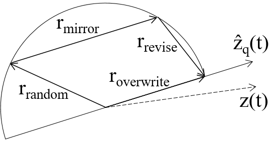

Intuitively, as the mirror operation is just adding an extra complex number being approximately parallel to the current DMF, it would generate much less effect to the original random walks in the orthogonal direction of the current DMF than that of the overwriting operation. Meanwhile, if the strength of the measured DMF is always in , as the samplings of the random variable are evenly distributed in , the expectation of the additional strength contributed by the mirror operation in a single step of the walk would be , as is shown in Fig. 1c. With this, if the changes of the directions of the DMF are no larger than during the -step walk, the strength of the DMF can grow to easily.
So, by configuring with some small linear coefficient, we expect that the system can reach a deterministic state with a high probability. To this, we provide some simple numerical simulation results with randomly posed without considering measurement errors and malign faults. As the measurement errors are bounded, and the effect of in changing the direction of the current moving curve would be fast filtered out, these results also make some sense in considering the general cases with arbitrarily posed . Firstly, by configuring and with being the number of the steps of the random walk observed in the -window, the extended half-random-walk DMF can reach the desired strength with very high probabilities. As is shown in Fig. 2, by setting and running only -step simulation (i.e., with records in every -window and running every simulation for a duration), fast stabilization is observed in all performed simulations (several instances), where the DMF in all simulations are ended with the strength close to .


As a comparison, when the two parameters and are configured larger or smaller, the strength of the DMF might not always be fast converged to in -windows. For example, when is configured as (the other settings are the same), the strength can be still in the range after -windows with a manifestable probability, as is shown in Fig. 3. For another example, when is configured as , the walks show random behavior at the end of the simulations with a manifestable probability, as is shown in Fig. 4. Nevertheless, even with these larger and smaller parameters, the probabilities of system stabilization in -windows are still very high.


For the overall synchronization, with the strength of the DMF being more than with a very high probability after several -windows, the precision can be approximately with being the maximal errors in measuring the DMF. So can be improved by taking a larger (the number of items in the -window) at the expense of a longer startup time (in running the first several durations).
6. Realizations
One practical problem with the basic DMF-based synchronization scheme might be the required trigonometric functions. Here we show how to overcome this computation problem with a prototype system realization.
This basic realization is developed upon distributed computers connected with standard switched Ethernet to show the DMF-based synchronization’s basic applicability. Concretely, distributed nodes are configured as independent Linux kernel modules run in two computers with the Ubuntu16.04LTS (ubu 2016) operating systems. Each node is scheduled to broadcast TT-frames at some pre-configured time-slots periodically. To enhance the real-time properties of the system, we disable the power-save features of the CPUs, modify the NIC-driver codes in the kernel space, and make high-precision time readings. Meanwhile, necessary atomic instructions and locks are also used to avoid resource access conflicts in each computer. A full-duplex standard best-effort Ethernet switch connects the computers with a negotiated speed of 1000Mbps.
During initialization, each node is normally started with an empty queue of the recorded pulses. Then, whenever the synchronization phase of reaches a pre-configured broadcasting phase (being different in different nodes), would broadcast a TT-frame. Thus, on the one hand, the synchronization phases are expected to be synchronized by tracing the phase-angles of the DMF. The DMF, on the other hand, is measured in every by just receiving the TT-frames from other nodes (by subtracting the pre-configured broadcasting phase of from the receiving instant of the frame from ).
In realizing the DMF-based synchronization, as no floating-point numbers nor trigonometric functions are supported in the Linux kernel spaces, we have manually realized some lightweight trigonometric functions in the kernel. These trigonometric functions only use integers to calculate and represent the input and output values, and thus can run much faster than the common trigonometric functions realized in glibc2.23 (gli 2016). Then, in further simplifying these functions, we use the -norm unit circle to replace the -norm unit circle in simulating the sine and cosine functions. Similarly, the -argument arctangent functions can also be approximated by simple facets in the -dimensional space. Most simply, we use radially symmetrical facets, which make a continuous zigzag-surface and also have zero values when the phase-angle is , to replace the original smooth surface of the -argument arctangent functions. More segments and facets can also be added to obtain lower approximation errors.
In verifying the basic applicability of the DMF-based synchronization, the experiments shown in Fig. 5 run with the simplest realization of the trigonometric functions and a trivial startup of the initial DMF (without any faulty nodes). The frames are observed in a third computer connected to the switch to measure the synchronization results approximately. In Fig. 5, it shows that whenever the system is synchronized by the DMF, all the TT-frames can be received from the standard Ethernet switch with the pre-configured broadcasting phases. Thus, we can see that the DMF-based synchronization can be easily realized in the presence of non-ignorable communication delays without common trigonometric functions.


7. Conclusion
In this paper, we have proposed the DMF-PRW synchronization scheme by integrating classical PRW with some additional operations. Firstly, by introducing PRW into the ABD pulsing systems, we have proposed a way to utilize the classical result of PRW in establishing the initial synchronization with an expected sqrt-strength DMF. For an intuitive example, we have shown that the authenticated one-kick DMF synchronization can trivially reach and maintain the synchronized state of the system for a bounded duration with some fixed probabilities. Then, we have provided several kinds of anonymous DMF to construct more practical synchronization systems by introducing the mirror, revising, and other possible operations. With a simplified analysis of the basic half-random-walk system, we have shown that the effect of in changing the direction of the DMF would be filtered out with an exponential convergence rate. With this, we have also shown that the strength of the DMF can reach with a constant positive probability. Thus the synchronization system can reach stabilization in an expected constant number of -windows. Meanwhile, by introducing the mirror operation, we have shown that the strength of the DMF can fast grow to with a high probability, with which the revising operation can further bring the DMF to the maximal strength. With numeric simulations, we have shown that by properly configuring the core parameters, the half-random-walk synchronization can be reached in a constant number of -windows with very high probabilities. Lastly, we have also provided a prototype realization and shown the basic applicability of the DMF-PRW synchronization without the support of common trigonometric functions. As the pulsing-frequency restriction can be eliminated in wired systems, these results can be extended to wired message-passing systems without difficulties.
Despite the current results of the proposed system, several problems with the DMF-PRW synchronization scheme need to be further investigated. Firstly, with a better investigation of the anonymous pulses generated in nonfaulty nodes, we wonder if the length of the -windows can be reduced to a constant number being independent of and , especially with . Secondly, the analysis of the half-random-walk synchronization system still relies on some informal arguments in integrating the classical eigenvalue analysis with planar random walks, especially in discussing the effects of past random walk inputs in changing the directions of the DMF. This can be further improved with better investigation of the planar random walks. Thirdly, the integration of the half-random-walk system with other operations such as approximate agreements (Dolev et al. 1986b) can be further explored to enhance resilience in the stabilized systems. In considering real-world applications, firstly, as the actual physical pulses are often generated with noises, the DMF-PRW synchronization solutions should better be extended to handle the general PRW with random-length steps (Wade and Xu 2015; McRedmond and Wade 2018). Secondly, as real-world communication networks are often partially connected, the stabilization properties of the DMF-PRW synchronization systems in partially connected networks need to be further studied. Besides, by viewing the synchronized sub-networks as super-nodes in the larger networks, the scaling of system-sizes can also be further investigated with the DMF-PRW synchronization scheme.
References
- (1)
- gli (2016) 2016. glibc. https://sourceware.org/glibc. [Online; accessed 12-Jul-2018].
- ubu (2016) 2016. ubuntu. https://ubuntu.com/. [Online; accessed 8-May-2018].
- Ademaj et al. (2003) Astrit Ademaj, Håkan Sivencrona, Günther Bauer, and Jan Torin. 2003. Evaluation of Fault Handling of the Time-Triggered Architecture with Bus and Star Topology. In In IEEE International Conference on Dependable Systems and Networks.
- Ashkiani and Scaglione (2012) Saman Ashkiani and Anna Scaglione. 2012. Discrete Dithered Desynchronization. Computer Science (2012).
- Borwein et al. (2010) Jonathan M Borwein, Dirk Nuyens, Armin Straub, and James Wan. 2010. Random Walks in the Plane. FPSAC 2010, San Francisco, USA (2010), 191–202.
- Buck and Buck (1966) John Buck and Elisabeth Buck. 1966. Biology of Synchronous Flashing of Fireflies. Nature 211, 5049 (1966), 562–564. https://doi.org/10.1038/211562a0
- Buck and Buck (1968) J. Buck and E. Buck. 1968. Mechanism of Rhythmic Synchronous Flashing of Fireflies: Fireflies of Southeast Asia may use anticipatory time-measuring in synchronizing their flashing. Science 159, 3821 (1968), 1319–1327. https://doi.org/10.1126/science.159.3821.1319
- Buranapanichkit et al. (2015) D. Buranapanichkit, N. Deligiannis, and Y. Andreopoulos. 2015. Convergence of Desynchronization Primitives in Wireless Sensor Networks: A Stochastic Modeling Approach. IEEE Transactions on Signal Processing 63, 1 (2015), 221–233. https://doi.org/10.1109/TSP.2014.2369003
- Daliot et al. (2003) Ariel Daliot, Danny Dolev, and Hanna Parnas. 2003. Self-Stabilizing Pulse Synchronization Inspired by Biological Pacemaker Networks. In Proceedings of the 6th International Conference on Self-Stabilizing Systems (San Francisco, CA, USA) (SSS’03). Springer-Verlag, Berlin, Heidelberg, 32–48. https://doi.org/10.1007/3-540-45032-7_3
- Degesys and Nagpal (2008) J. Degesys and R. Nagpal. 2008. Towards Desynchronization of Multi-hop Topologies. SASO 2008: Second IEEE International Conference on Self-Adaptive and Self-Organizing Systems, Proceedings (2008), 129–138. https://doi.org/10.1109/Saso.2008.70
- Degesys et al. (2007) J. Degesys, I. Rose, A. Patel, and R. Nagpal. 2007. DESYNC: Self-organizing desynchronization and TDMA on wireless sensor networks. Proceedings of the Sixth International Symposium on Information Processing in Sensor Networks (2007), 11–20. https://doi.org/10.1145/1236360.1236363
- Degesys et al. (2008) J. Degesys, I. Rose, A. Patel, and R. Nagpal. 2008. Self-organizing Desynchronization and TDMA on Wireless Sensor Networks. Bio-Inspired Computing and Communication 5151 (2008), 192–203.
- Dolev (1982) D. Dolev. 1982. The Byzantine Generals Strike Again. Journal of Algorithms 3, 1 (1982), 14–30. https://doi.org/10.1016/0196-6774(82)90004-9
- Dolev et al. (2014) D. Dolev, M. Fugger, U. Schmid, and C. Lenzen. 2014. Fault-Tolerant Algorithms for Tick-Generation in Asynchronous Logic: Robust Pulse Generation. Journal of the Acm 61, 5 (2014). https://doi.org/10.1145/2560561
- Dolev et al. (1986a) D. Dolev, J. Y. Halpern, and H. R. Strong. 1986a. On the Possibility and Impossibility of Achieving Clock Synchronization. J. Comput. System Sci. 32, 2 (1986), 230–250. https://doi.org/10.1016/0022-0000(86)90028-0
- Dolev and Hoch (2007) Danny Dolev and Ezra N. Hoch. 2007. Byzantine Self-stabilizing Pulse in a Bounded-Delay Model. In Stabilization, Safety, and Security of Distributed Systems, Toshimitsu Masuzawa and Sébastien Tixeuil (Eds.). Springer Berlin Heidelberg, Berlin, Heidelberg, 234–252. https://doi.org/10.1007/978-3-540-76627-8_19
- Dolev et al. (1986b) D. Dolev, N. A. Lynch, S. S. Pinter, E. W. Stark, and W. E. Weihl. 1986b. Reaching Approximate Agreement in the Presence of Faults. Journal of the Acm 33, 3 (1986), 499–516. https://doi.org/10.1145/5925.5931
- Dolev and Welch (2004) Shlomi Dolev and Jennifer L. Welch. 2004. Self-Stabilizing Clock Synchronization in the Presence of Byzantine Faults. J. ACM 51, 5 (Sept. 2004), 780–799. https://doi.org/10.1145/1017460.1017463 A former version appears in Proc. of the Second Workshop on Self-Stabilizing Systems, pp. 9.1–9.12, Abstract in Proc. of the 14th Annual ACM Symp. on Principles of Distributed Computing.
- Dorfler and Bullo (2014) F. Dorfler and F. Bullo. 2014. Synchronization in complex networks of phase oscillators: A survey. Automatica 50, 6 (2014), 1539–1564. https://doi.org/10.1016/j.automatica.2014.04.012
- Feldman and Micali (1989) Paul Feldman and Silvio Micali. 1989. An optimal probabilistic algorithm for synchronous Byzantine agreement. In Automata, Languages and Programming, Giorgio Ausiello, Mariangiola Dezani-Ciancaglini, and Simonetta Ronchi Della Rocca (Eds.). Springer Berlin Heidelberg, Berlin, Heidelberg, 341–378. https://doi.org/10.1007/BFb0035770
- Feldman and Micali (1997) Pesech Feldman and Silvio Micali. 1997. An Optimal Probabilistic Protocol for Synchronous Byzantine Agreement. SIAM J. Comput. 26, 4 (Aug. 1997), 873–933. https://doi.org/10.1137/S0097539790187084
- Ferrante and Wang ([n.d.]) F. Ferrante and Y. Wang. [n.d.]. A hybrid systems approach to splay state stabilization of pulse coupled oscillators. In 2016 IEEE 55th Conference on Decision and Control (CDC). 1763–1768. https://doi.org/10.1109/CDC.2016.7798520
- Ferrante and Wang (2017) F. Ferrante and Y. Wang. 2017. Robust Almost Global Splay State Stabilization of Pulse Coupled Oscillators. IEEE Trans. Automat. Control 62, 6 (2017), 3083–3090. https://doi.org/10.1109/TAC.2017.2677740
- Friesen (1975a) W. Otto Friesen. 1975a. Physiological anatomy and burst pattern in the cardiac ganglion of the spiny lobsterPanulirus interruptus. Journal of Comparative Physiology 101, 3 (1975), 173–189. https://doi.org/10.1007/bf00657180
- Friesen (1975b) W. Otto Friesen. 1975b. Synaptic interactions in the cardiac ganglion of the spiny lobsterPanulirus interruptus. Journal of Comparative Physiology 101, 3 (1975), 191–205. https://doi.org/10.1007/bf00657181
- Fugger et al. (2006) Matthias Fugger, Ulrich Schmid, Gottfried Fuchs, and Gerald Kempf. 2006. Fault-Tolerant Distributed Clock Generation in VLSI Systems-on-Chip. In Proceedings of the Sixth European Dependable Computing Conference (EDCC ’06). IEEE Computer Society, USA, 87–96. https://doi.org/10.1109/EDCC.2006.11
- Gao and Wang (2017) H. Gao and Y. Wang. 2017. On Phase Response Function Based Decentralized Phase Desynchronization. IEEE Transactions on Signal Processing 65, 21 (2017), 5564–5577. https://doi.org/10.1109/TSP.2017.2733452
- Gentz et al. (2016) R. Gentz, A. Scaglione, L. Ferrari, and Y. W. P. Hong. 2016. PulseSS: A Pulse-Coupled Synchronization and Scheduling Protocol for Clustered Wireless Sensor Networks. IEEE Internet of Things Journal 3, 6 (2016), 1222–1234. https://doi.org/10.1109/JIOT.2016.2576923
- Hinterhofer et al. (2012) T. Hinterhofer, H. P. Schwefel, and S. Tomic. 2012. RD2: Resilient Dynamic Desynchronization for TDMA over Lossy Networks. 2012 31st International Symposium on Reliable Distributed Systems (Srds 2012) (2012), 231–236. https://doi.org/10.1109/Srds.2012.57
- Hong and Scaglione (2003) Yao-Win Hong and Anna Scaglione. 2003. Time synchronization and reach-back communications with pulse-coupled oscillators for UWB wireless ad hoc networks. In IEEE Conference on Ultra Wideband Systems and Technologies, UWBST 2003. 190 – 194. https://doi.org/10.1109/UWBST.2003.1267830
- Hong and Scaglione (2005) Y. W. Hong and A. Scaglione. 2005. A scalable synchronization protocol for large scale sensor networks and its applications. Ieee Journal on Selected Areas in Communications 23, 5 (2005), 1085–1099. https://doi.org/10.1109/Jsac.2006.845418
- Huygens (1665) C. Huygens. 1665. Letters to de Sluse, (letters; no. 1333 of 24 February 1665, no. 1335 of 26 February 1665, no. 1345 of 6 March 1665). (Societe Hollandaise Des Sciences, Martinus Nijho, 1895) (1665).
- Kang and Wong (2009) H. Kang and J. L. Wong. 2009. A Localized Multi-Hop Desynchronization Algorithm for Wireless Sensor Networks. Ieee Infocom 2009 - Ieee Conference on Computer Communications, Vols 1-5 (2009), 2906–2910. https://doi.org/10.1109/Infcom.2009.5062256
- Konishi and Kokame (2008) K. Konishi and H. Kokame. 2008. Synchronization of pulse-coupled oscillators with a refractory period and frequency distribution for a wireless sensor network. Chaos 18, 3 (2008). https://doi.org/Artn03313210.1063/1.2970103
- Kuramoto (1984) Yoshiki Kuramoto. 1984. Chemical Oscillations, Waves, and Turbulence. Springer Verlag. https://doi.org/10.1007/978-3-642-69689-3
- Lenzen and Rybicki (2019) C. Lenzen and J. Rybicki. 2019. Self-Stabilising Byzantine Clock Synchronisation Is Almost as Easy as Consensus. Journal of the Acm 66, 5 (2019). https://doi.org/10.1145/3339471
- Lord Rayleigh (1880) F.R.S. Lord Rayleigh. 1880. On the resultant of a large number of vibrations of the same pitch and of arbitrary phase. The London, Edinburgh, and Dublin Philosophical Magazine and Journal of Science 10, 60 (1880), 73–78. https://doi.org/10.1080/14786448008626893
- Mauroy et al. (2012) A. Mauroy, P. Sacre, and R. Sepulchre. 2012. Kick synchronization versus diffusive synchronization. 2012 Ieee 51st Annual Conference on Decision and Control (Cdc) (2012), 7171–7183.
- McRedmond and Wade (2018) James McRedmond and Andrew R. Wade. 2018. The convex hull of a planar random walk: perimeter, diameter, and shape. Electronic Journal of Probability 23, none (2018), 1 – 24. https://doi.org/10.1214/18-EJP257
- Mirollo and Strogatz (1990) R. E. Mirollo and S. H. Strogatz. 1990. Synchronization of Pulse-Coupled Biological Oscillators. Siam Journal on Applied Mathematics 50, 6 (1990), 1645–1662. https://doi.org/10.1137/0150098
- Nunez et al. (2015a) F. Nunez, Y. Q. Wang, and F. J. Doyle. 2015a. Global synchronization of pulse-coupled oscillators interacting on cycle graphs. Automatica 52 (2015), 202–209. https://doi.org/10.1016/j.automatica.2014.10.111
- Nunez et al. (2015b) F. Nunez, Y. Q. Wang, and F. J. Doyle. 2015b. Synchronization of Pulse-Coupled Oscillators on (Strongly) Connected Graphs. Ieee Transactions on Automatic Control 60, 6 (2015), 1710–1715. https://doi.org/10.1109/Tac.2014.2361196
- Núñez et al. ([n.d.]) F. Núñez, Y. Wang, and F. J. Doyle. [n.d.]. Bio-inspired hybrid control of pulse-coupled oscillators and application to synchronization of a wireless network. In 2012 American Control Conference (ACC). 2818–2823. https://doi.org/10.1109/ACC.2012.6314981
- Okuda et al. (2011) T. Okuda, K. Konishi, and N. Hara. 2011. Experimental verification of synchronization in pulse-coupled oscillators with a refractory period and frequency distribution. Chaos 21, 2 (2011). https://doi.org/Artn02310510.1063/1.3559135
- Pagliari et al. (2010) R. Pagliari, Y. W. P. Hong, and A. Scaglione. 2010. Bio-Inspired Algorithms for Decentralized Round-Robin and Proportional Fair Scheduling. Ieee Journal on Selected Areas in Communications 28, 4 (2010), 564–575. https://doi.org/10.1109/Jsac.2010.100506
- Pagliari and Scaglione (2011) R. Pagliari and A. Scaglione. 2011. Scalable Network Synchronization with Pulse-Coupled Oscillators. IEEE Transactions on Mobile Computing 10, 3 (2011), 392–405. https://doi.org/10.1109/TMC.2010.171
- Patel et al. (2007) A. Patel, J. Degesys, and R. Nagpal. 2007. Desynchronization: The theory of self-organizing algorithms for round-robin scheduling. First Ieee International Conference on Self-Adaptive and Self-Organizing Systems (2007), 87–+. https://doi.org/10.1109/Saso.2007.17
- Pearson (1905) Karl Pearson. 1905. The Problem of the Random Walk. Nature 72, 1865 (1905), 294–294. https://doi.org/10.1038/072294b0
- Peskin (1975) C. S. Peskin. 1975. Mathematical Aspects of Heart Physiology.
- Powell (1992) D. Powell. 1992. Failure mode assumptions and assumption coverage. In [1992] Digest of Papers. FTCS-22: The Twenty-Second International Symposium on Fault-Tolerant Computing. 386–395. https://doi.org/10.1109/FTCS.1992.243562
- Steiner (2008) Wilfried Steiner. 2008. Startup and Recovery of Fault-Tolerant Time-Triggered Communication: With a Focus on Bus-Based and Switch-Based Network Topologies. VDM Verlag Dr. Müller. 160 pages.
- Wade and Xu (2015) Andrew R. Wade and Chang Xu. 2015. Convex hulls of random walks and their scaling limits. Stochastic Processes and their Applications 125, 11 (2015), 4300–4320. https://doi.org/10.1016/j.spa.2015.06.008
- Wang and F. J. Doyle (2012) Y. Wang and III F. J. Doyle. 2012. Optimal Phase Response Functions for Fast Pulse-Coupled Synchronization in Wireless Sensor Networks. IEEE Transactions on Signal Processing 60, 10 (2012), 5583–5588. https://doi.org/10.1109/TSP.2012.2208109
- Wang et al. (2012) Y. Wang, F. Nunez, and F. J. Doyle. 2012. Energy-Efficient Pulse-Coupled Synchronization Strategy Design for Wireless Sensor Networks Through Reduced Idle Listening. IEEE Transactions on Signal Processing 60, 10 (2012), 5293–5306. https://doi.org/10.1109/TSP.2012.2205685
- Wang et al. (2013) Y. Wang, F. Núñez, and F. J. Doyle. 2013. Increasing Sync Rate of Pulse-Coupled Oscillators via Phase Response Function Design: Theory and Application to Wireless Networks. IEEE Transactions on Control Systems Technology 21, 4 (2013), 1455–1462. https://doi.org/10.1109/TCST.2012.2205254
- Wang and Wang (2018a) Z. Wang and Y. Wang. 2018a. Attack-Resilient Pulse-Coupled Synchronization. IEEE Transactions on Control of Network Systems (2018), 1–1. https://doi.org/10.1109/TCNS.2018.2817922
- Wang and Wang (2018b) Z. Wang and Y. Wang. 2018b. Pulse-Coupled Oscillators Resilient to Stealthy Attacks. IEEE Transactions on Signal Processing 66, 12 (2018), 3086–3099. https://doi.org/10.1109/TSP.2018.2824285
- Wang and Wang (2020) Zhenqian Wang and Yongqiang Wang. 2020. Global Synchronization of Pulse-Coupled Oscillator Networks Under Byzantine Attacks. IEEE Transactions on Signal Processing PP (05 2020), 1–1. https://doi.org/10.1109/TSP.2020.2993643
- Winfree (1967) Arthur T. Winfree. 1967. Biological rhythms and the behavior of populations of coupled oscillators. Journal of Theoretical Biology 16, 1 (1967), 15–42. https://doi.org/10.1016/0022-5193(67)90051-3
- Winfree (1980) Arthur T. Winfree. 1980. The geometry of biological time. Springer Verlag. https://doi.org/10.1007/978-1-4757-3484-3
- Winfree (1987) Arthur T. Winfree. 1987. Timing of Biological Clocks. Scientific American Press.