Amplitude-Constrained Constellation and Reflection Pattern Designs for Directional Backscatter Communications Using Programmable Metasurface

Fig. 1 shows the working mechanism of programmable metasurfaces. A dedicated incident signal $E_{i}(t)$ impinges on the metasurface, and the reflected signal ${E}_{r}(t)$ can be configured by the controller via tuning the load impedance. Following [15, 16], the incident signal considered is emitted by a dedicated power source and is a single-tone sinusoidal¹¹ 1 In accordance with [15, 16], we assume that the programmable metasurface is placed in the far field of the horn antenna. Thus, the incident signal $E_{i}(t)$ is identical for all the metasurface units. , i.e., $E_{i}(t)=A\cos(2\pi f_{c}t+\varphi_{0})$, and thus the reflected signal ${E}_{r}(t)$ is a single-tone carrier signal as well.

Applying phasor method in circuit analysis, we obtain the relationship between the incident signal and the reflected signal as follows

where $\mathbb{E}_{i}=Ae^{j\varphi_{0}}$ is the phasor-domain representation (in exponential form) of the incident signal $E_{i}(t)$, $\mathbb{E}_{r}$ is the phasor-domain representation of the reflected signal $E_{r}(t)$, and $\Gamma$ is the reflection coefficient that describes the fraction of the electromagnetic wave reflected by an impedance discontinuity in the transmission medium [15, 28, 29], and $\Gamma(\omega)=|\Gamma(\omega)|e^{j\varphi_{\Gamma(\omega)}}$ denotes the exact value of the reflection coefficient when the angular frequency is $\omega=2\pi f_{c}$. To be concise, $\omega$ will be omitted in the following context. According to [30, 29, 31, 15], the expression of the reflection coefficient is given by

where $Z_{l}$ is the equivalent load impedance of metasurface unit, and $Z_{0}$ is the impedance of air. Through tuning $Z_{l}$, the magnitude and phase of the reflection coefficient $\Gamma$ can be configured by the controller of programmable metasurface [30], and the exact value of the load impedance $Z_{l}$ can be derived via the well-known Smith chart.

Owing to the physical property of passive reflection, the reflection coefficient $\Gamma$ satisfies

To explore the theoretical performance upper bound of the backscatter communications, we neglect the current hardware constraints [19, 16] and assume that the amplitude and the phase of the reflection coefficient can be tuned independently and continuously under the constraint (3). Thus, the magnitude of the reflected signal satisfies

In the realm of telecommunications, ${\mathbb{E}}_{r}$ is also referred to as equivalent baseband signal of the reflected signal ${E}_{r}(t)$. Thus, (4) indicates that the baseband signal of backscatter modulation is amplitude constrained, which is different from the power constraint imposed on the traditional communication systems.

Backscatter modulation is realized by changing the reflection coefficient according to the input information. In order to convey information, the reflection coefficient is configured as

where $\Gamma[m]$ is selected from a pre-designed finite alphabet, i.e., $\Gamma[m]\in\{I_{1},I_{2},\cdots,I_{|\mathcal{S}|}\}$, according to the input information bits, $h(t)$ is the rectangular pulse, and $T$ is symbol duration.

Thus, the constellation alphabet of the equivalent baseband signal ${\mathbb{E}}_{r}$ is given by

According to (4), the constellation of programmable metasurface enabled backscatter communications is under an amplitude constraint, i.e.,

Although the amplitude of the reflected signal can be changed by controlling the transmit power of the horn antenna to obey the conventional power constraint, this structure requires (1) the strict synchronization between the programmable metasurface and the horn antenna, (2) the amplitude modulation capacity of the horn antenna, and (3) the linear wideband power amplifier for amplitude modulation at the horn antenna side. Also, the amplitude of all the metasurface units can only be controlled collectively. In a word, amplitude control at horn antenna side is not cost-effective and does not fully utilize the advantages of programmable metasurfaces. Thus, we follow the structure proposed by [15, 16] in our work and let the horn antenna simply provide an incident pure carrier signal.

A salient advantage of programmable metasurfaces over the conventional backscatter antennas is its capability of directional beamforming, which is brought by the large number of metasurface units. Concatenating the incident and reflected signal of the $N$ metasurface units, we have the vector-form representation of (1) as

where $\mathbf{f}$ is the reflection coefficient vector, and, according to (3), $\mathbf{f}$ follows the amplitude constraint, i.e.,

When $\mathbf{f}=\mathbf{1}$, the reflection pattern is omni-directional, which is apparently energy inefficient. Since the intended users of backscatter communications are usually distributed in a constrained area, e.g., a plaza, a street block, a road section, the ideal reflection pattern should be concentrated and homogeneous within the interested area.

We assume that the metasurface units are arranged as an $N_{x}\times N_{y}$ rectangular planar array, and the array response vector of programmable metasurface is represented as

and

where $\Psi_{x}$ and $\Psi_{y}$ are cosine of the angle of arrival/depature (AoA/AoD), a.k.a. direction cosines, [32, 33]. To maximize the reflected signal power within the interested angle range and guarantee uniform signal strength, i.e., beam homogenization, in the meantime, we propose the following design criteria.

Criterion 2: Minimized the ripple factor within the intended angle range $[\theta_{L},\;\theta_{U})$, namely

where

and $P_{\mathcal{D}_{\Psi}}$ is the power of the reflected signal within the intended angle range $\mathcal{D}_{\Psi}$, $V_{Mean}$ is the mean voltage of the reflected signal over the intended angle range $\mathcal{D}_{\Psi}$, $V_{Ripple}$ is root mean square (RMS) of the ripple voltage, $\frac{V_{Ripple}}{V_{Mean}}$ is the ripple factor that measures the degree of fluctuations over the intended angle range $\mathcal{D}_{\Psi}$, and $\mathcal{A}(\mathcal{D}_{\Psi})$ is the area of $\mathcal{D}_{\Psi}$.

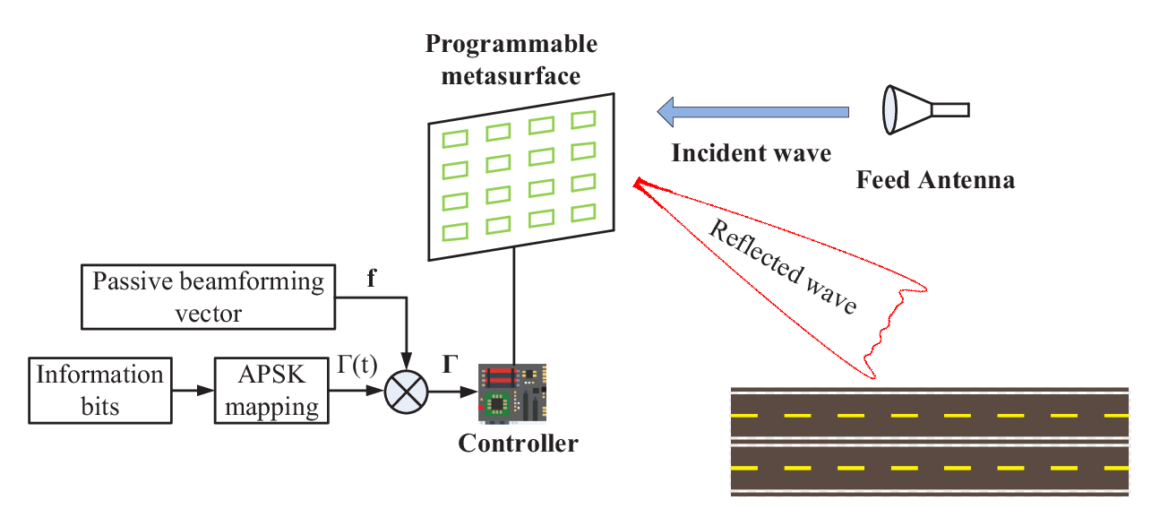
Fig. 2 shows the working mechanism of signal modulation in programmable metasurface enabled backscatter communications. A single-tone carrier signal $E_{i}(t)$ impinges on the programmable metasurface from a feed antenna. Signal modulation is realized by collectively changing the reflection coefficients of programmable metasurface according to the incoming information bits, and passive beamforming is realized by imposing beamforming vector on the metasurface units. Thus, the reflection coefficient of directional backscatter communications can be represented as the product of the information-bearing factor $\Gamma(t)$ in (5) and the passive beamforming factor $\mathbf{f}$ (refer to (8)), i.e.,

Note that $\Gamma(t)$, which is decided by the incoming information bits, is time-variant, and $\mathbf{f}$, which determines the reflection pattern, is pre-designed and time-invariant. For example, when a programmable metasurface is deployed on a building, and its intended receivers are the vehicles, the reflection pattern is designed to cover the road section in front of the building as shown in Fig. 2.

When the constellation of backscatter communications satisfies the amplitude constraint in (7) and the passive beamforming vector $\mathbf{f}$ satisfies the amplitude constraint in (9), the synthesized $\bm{\Gamma}$ will meet the amplitude constraint and thus can be readily applied to realize directional backscatter communications. Similar to the conventional MIMO with precoding/beamforming [34, 35], where the design of transmit signals fed to multiple antennas is disentangled into the constellation design and the precoding/beamforming vector design, the optimization of the reflection coefficient vector $\bm{\Gamma}$ can be also decomposed into two independent sub-problems of constellation design and passive beamforming design, given that the amplitude constraint is satisfied by the two sub-problems.

To summarize, in this paper, we will carry out (I) the design of the constellation alphabet $\mathcal{S}$ under the amplitude constraint (7) and (II) the design of the reflection pattern (namely, the passive beamforming vector $\mathbf{f}$) under the amplitude constraint (9) to optimize the performance of directional backscatter communications using programmable metasurface.

Owing to its design flexibility, APSK has been widely used in practical communications systems, e.g., DVB-S2 [36], and MIMO precoding design under constant envelope constraint [37] to provide a power and spectral efficient solution. APSK conveys information through changing both the amplitude and the phase of the carrier signal. APSK with different parameters can be used to represent PSK and QAM. Thus, APSK can be regarded as a unified modulation scheme. In this paper, we propose to optimize the constellation parameters for APSK in programmable metasurface enabled backscatter communications.

The constellation points of APSK are distributed in two or more concentric rings. For example, $2$-ring 16-APSK constellation with $N_{1}=8$ points in the outer ring and $N_{2}=8$ points in the inner ring is shown in Fig. 3 and $2$-ring 16-APSK constellation with $N_{1}=10$ points in the outer ring and $N_{2}=6$ points in the inner ring is shown in Fig. 3. In a general case, consider an $L$-ring APSK constellation, the elements of which are represented as

where $l\in\{1,\cdots,L\}$ is the index of the ring, $L$ is the number of the rings, $k_{l}\in\{0,\cdots,N_{l}-1\}$ is the index of the constellation points in the $l$-th ring, $N_{l}$ is the number of constellation points in the $l$-th ring, $r_{l}$ is the radius of the $l$-th ring, and $\omega_{l}\in[0,\frac{2\pi}{N_{l}})$ is the phase of the reference constellation point (i.e., $k_{l}=0$) in the $l$-th ring. For APSK, the amplitude constraint (7) is rewritten as

The performance of signal constellation is dependent on the minimum distance between any pairs of constellation points [38], i.e.,

Thus, combining (17) and (18), the design criterion of APSK constellation in programmable metasurface enabled backscatter communications is formulated as

For APSK, the minimum Euclidean distance $d_{min}$ in (18) can be further represented as

where

is the intra-ring minimum Euclidean distance of the $l$-th ring, and

is the inter-ring minimum Euclidean distance between the constellation points in the $l$-th ring and the constellation points in the $\hat{l}$-th ring, where

is the minimum phase difference between the constellation points in the two rings.

With (24) and (25), P1 is rewritten by

where the parameters $L,\{{r}_{l}\},\{\omega_{l}\},\{N_{l}\}$ are the variables to be optimized. As the ranges of the integer variables $L,\{N_{l}\}$ are typically small, P2 can be resolved by firstly optimizing $\{r_{l}\},\{\omega_{l}\}$ with a given set of $L,\{N_{l}\}$, and then exhaustively searching over the feasible region of $L,\{N_{l}\}$. In addition, as the outermost ring corresponds to the best reflectivity, from an energy-greedy perspective, the optimal radius of the outermost ring is apparently $r_{L}^{*}=A$. The constraint of inter-ring distance is indeed a solvable linear constraint. However, the constraint of intra-ring distance is non-trivial, which can be written in quadratic form as follows

Obviously, it is a non-convex quadratic constraint w.r.t. $[r_{l},r_{\hat{l}}]^{T}$ that renders P2 challenging.

To make P2 tractable, we make the assumption that the minimum Euclidean distance is the assumptions that
(1) when $N_{1}\geq 2$, the minimum Euclidean distance is

(2) when $N_{1}=1$ (i.e., there is a constellation point in the center of the ring), the minimum Euclidean distance is

In addition, we can drop the constraint $r_{L}\leq A$ to obtain a set of intermediate radius parameters ${\hat{r}_{l}}$, and then normalize the intermediate radius parameters as

to meet the constraint. Without loss of generality, we can set $\hat{r}_{1}=1$ (or $\hat{r}_{2}=1$ when $N_{1}=1$).

Combining (37), (38) with (39), the objective of maximizing $d_{min}$ is reduced to minimizing $\hat{r}_{L}$. Thus, with a given set of $L$ and $\{N_{l}\}$, the optimization problem can be represented as

By decomposing P3 into $L-1$ subproblems, i.e.,

we can solve the problem in a recursive manner starting from the innermost ring ($l=1$) to the outermost ring ($l=L$). Note that the inter-ring Euclidean distance constraint is relaxed by neglecting ${d}_{min\_inter}(\hat{l},l+1)\geq{d}_{min},\;\forall\hat{l}<l$, as the inter-ring Euclidean distance between adjacent rings, i.e., ${d}_{min\_inter}(l,l+1)$, is usually smaller than the inter-ring Euclidean distance between non-adjacent rings, i.e., ${d}_{min\_inter}(\hat{l},l+1)$, where $\hat{l}<l$.

According to P4, $\omega_{l+1}$ merely relates to the inter-ring Euclidean distance, while $\hat{r}^{*}_{l+1}$ is related to both the inter-ring Euclidean distance and the intra-ring Euclidean distance. Thus, we will optimize $\omega_{l+1}$ and $\hat{r}_{l+1}$, successively.

With the solutions to P4, parameters of the optimal APSK can be obtained by exhaustively searching over the feasible set of $L$ and $\{N_{l}\}$. To narrow down the search range, we add the constraint $N_{1}\leq N_{2}\leq\cdots\leq N_{L}$ on $\{N_{l}\}$. To summarize, the procedures of our proposed APSK constellation design are summarized in Algorithm 1.

We assume that the intended angle range is $\mathcal{D}_{\Psi}=[\Psi_{x}^{L},\Psi_{x}^{U})\times[\Psi_{y}^{L},\Psi_{y}^{U})$, and thus the reflected power over $\mathcal{D}_{\Psi}$ is represented as

According to the mixed-product property of Kronecker product, the term $\mathbf{V}_{\mathcal{D}_{\Psi}}$ can be represented as

With respect to $\mathbf{V}_{\Psi_{x}}$, its $(\ell,\kappa)$-th entry is

which can be further represented as

Similarly, we derive the expression of the $(\ell,\kappa)$-th entry of $\mathbf{V}_{\Psi_{y}}$ as

We firstly review conventional beamforming techniques under sum power constraint, including fully digital beamforming, hybrid beamforming with multiple radio frequency (RF) chains, and hybrid beamforming with a single RF chain, and then discuss their compatibility with programmable metasurface enabled passive beamforming.

1) Fully digital beamforming

Review: Beam pattern design for fully digital beamforming has been well investigated in array signal processing [22, 23]. Similar to the design of finite impulse response (FIR) filters [39][40], window-based method [22] and least-square (LS) (or constrained least-square (CLS)) method [23, 26] can be readily applied to beam pattern designs. To accommodate the hardware structure, the length of the response needs to be equal to the number of array elements.

Compatibility: Beamforming vectors, including fully digital case, can meet the amplitude constraint of programmable metasurface enabled passive beamforming through normalizing $\mathbf{f}$ as follows

The normalized beamforming vector satisfies $\mathbf{f}^{H}\mathbf{f}=\frac{N}{\max_{n}|\mathbf{f}(n)|^{2}}$. According to Proposition 2, the sum power of the reflected signals is restricted by $\max_{n}|\mathbf{f}(n)|$, and thus a very large $\max_{n}|\mathbf{f}(n)|$ will result in a power-inefficient reflection pattern.

2) Hybrid beamforming with multiple RF chains

Review: Hybrid beamforming vector needs to be compatible with the hybrid digital and analog hardware structure. The key idea of beam pattern design for hybrid beamforming with multiple RF chains is to regenerate the reference beamforming vector, which is derived in fully digital case, under the hardware constraint. In [26], the reference beam pattern is firstly obtained through LS method and then approximated using orthogonal matching pursuit (OMP) algorithm. In [27], the reference beam pattern is firstly obtained through semidefinite relaxation (SDR) technique and then perfectly regenerated through vector decomposition.

Compatibility: As hybrid beamforming vector is an approximation of the desired digital beamforming vector (i.e., reference beamforming vector), its extension to reflection pattern design is the same as fully digital case.

3) Analog beamforming with a single RF chain

Review: Analog beamforming design with a single RF chain is performed under constant modulus constraint, which is brought by the analog phase shifter network. In [24, 25], subarray based beamforming designs are carried out for single-RF-chain array antenna. Through set partition, the element antennas are grouped as subarrays, and then subarrays with different directions are combined to synthesize beam patterns with different beamwidths. However, beamwidth of the subarray based method is confined to a few discrete values, which inevitably introduces a mismatch between the desired beamwidth and the actual beamwidth. In addition, half of the array elements have to be deactivated to attain some beamwidths using subarray based method.

Compatibility: The element of analog beamforming vector is either of constant modulus or zero-valued (deactivated). Analog beamforming vector can be readily applied to passive beamforming. The subarray based method [24, 25] generates two types of analog beamforming vectors. For Type 1, where all the analog phase shifters are activated, the beamforming vector satisfies $\mathbf{f}^{H}\mathbf{f}=N$; for Type 2, where half of the analog phase shifters are deactivated, the beamforming vector satisfies $\mathbf{f}^{H}\mathbf{f}=\frac{N}{2}$. Type 1 attains the maximum achievable reflection power, while Type 2 attains only half of the maximum achievable reflection power.

To fully exploit the reflectivity of programmable metasurface and achieve the maximum reflection power, we tighten the amplitude constraint $|\mathbf{f}(i)|\leq 1,\;\forall n\in\{1,..,N\}$ and incorporate the constant modulus constraint $|\mathbf{f}(i)|=1,\;\forall n\in\{1,..,N\}$ to reflection pattern design.

In addition, the reflection pattern design also aims to achieve the following two objectives.

Objective 1: Maximize the sum power of reflected signal over the intended angle range

Objective 2: Maximize the minimum power of reflected signal within the intended angle range

where

is the discrete grid of $(\Psi_{x},\Psi_{y})$ over the intended range $[\Psi_{x}^{L},\Psi_{x}^{U})\times[\Psi_{y}^{L},\Psi_{y}^{U})$ with the grid size $(\frac{2}{N_{x}},\frac{2}{N_{y}})$.

Note that Objective 1 and Objective 2 correspond to the design criterion 1 and design criterion 2 in Section II. C, respectively. To resolve the above multi-objective optimization problem, we apply the weighted sum method [41]. Specifically, we introduce a hyper-parameter $\alpha$ to combine Objective 1 and Objective 2 and formulate the new research problem as follows

where $\mathbf{M}_{\Psi_{x},\Psi_{y}}\triangleq\mathbf{v}(\Psi_{x},\Psi_{y})\mathbf{v}^{H}(\Psi_{x},\Psi_{y})+\alpha\mathbf{V}_{\mathcal{D}_{\Psi}}$.

For the angle range $\mathcal{D}_{\Psi}=[\Psi_{x}^{L},\Psi_{x}^{U})\times[\Psi_{y}^{L},\Psi_{y}^{U})$, P5 can be broken down into the subproblems w.r.t. $\Psi_{x}$ and $\Psi_{y}$. W.r.t. $\Psi_{x}$, the design problem is given as

W.r.t $\Psi_{y}$, the component vector $\mathbf{f}_{y}$ can be obtained in the similar way. Then, the beamforming vector can be derived as $\mathbf{f}=\mathbf{f}_{x}\otimes\mathbf{f}_{y}$.

We firstly focus on maximizing a specific term $\mathbf{f}_{x}^{H}\mathbf{M}_{\Psi_{x}}\mathbf{f}_{x}$ and then extend the method to the max-min problem [42].

The minimum Euclidean distance between different constellation points is a key performance indicator of the constellation, which determines its symbol error rate (SER), bit error rate (BER) and mutual information [44]. To this end, we make comparisons of the minimum Euclidean distance between the conventional QAM/PSK constellations and our optimized APSK constellation. We firstly list the parameters for the optimized APSK as follows and plot the constellations in Fig. 4.

• •

  When the modulation order is $M=8$, the parameters for the optimal APSK are $L=2$, $N_{1}=1,N_{2}=7$, $r_{1}=0,r_{2}=1$, and $\omega_{1}=0,\omega_{2}=0.4488$;

• •

  When the modulation order is $M=16$, the parameters for the optimal APSK are $L=2$, $N_{1}=5,N_{2}=11$, $r_{1}=0.4603,r_{2}=1$, $\omega_{1}=0,\omega_{2}=0.0571$;

• •

  When the modulation order is $M=32$, the parameters for the optimal APSK are $L=3$, $N_{1}=5,N_{2}=10,N_{3}=17$, $r_{1}=0.3068,r_{2}=0.6397,r_{3}=1$, $\omega_{1}=0,\omega_{2}=0.3142,\omega_{3}=0.3326$;

• •

  When the modulation order is $M=64$, the parameters for the optimal APSK are $L=5$, $N_{1}=1,N_{2}=6,N_{3}=13,N_{4}=19,N_{5}=25$, $r_{1}=0,r_{2}=0.2446,r_{3}=0.5110,r_{4}=0.7555,r_{5}=1$, $\omega_{1}=0,\omega_{2}=0.5236,\omega_{3}=0.5639,\omega_{4}=0.5766,\omega_{5}=0.5832$;

References

- [1] W. Liu, K. Huang, X. Zhou, and S. Durrani, “Next generation backscatter communication: systems, techniques, and applications,” EURASIP J. Wireless Commun. Netw., vol. 2019, no. 1, pp. 1–11, Mar. 2019.
- [2] C. Boyer and S. Roy, “Backscatter communication and RFID: Coding, energy, and MIMO analysis,” IEEE Trans. Commun., vol. 62, no. 3, pp. 770–785, Mar. 2014.
- [3] Q. Wu, S. Zhang, B. Zheng, C. You, and R. Zhang, “Intelligent reflecting surface-aided wireless communications: A tutorial,” IEEE Trans. Commun., vol. 69, no. 5, pp. 3313–3351, May 2021.
- [4] T. J. Cui, D. R. Smith, and R. Liu, Metamaterials: Theory, Design, and Applications. Springer, 2009.
- [5] H. Yang, X. Cao, F. Yang, J. Gao, S. Xu, M. Li, X. Chen, Y. Zhao, Y. Zheng, and S. Li, “A programmable metasurface with dynamic polarization, scattering and focusing control,” Sci. Rep., vol. 6, no. 1, pp. 1–11, Oct. 2016.
- [6] W. Wang and W. Zhang, “Joint beam training and positioning for intelligent reflecting surfaces assisted millimeter wave communications,” IEEE Trans. Wireless Commun., vol. 20, no. 10, pp. 6282–6297, Oct. 2021.
- [7] ——, “Intelligent reflecting surface configurations for smart radio using deep reinforcement learning,” IEEE J. Sel. Areas in Commun., vol. 40, no. 8, Aug. 2022.
- [8] S. Zhang and R. Zhang, “Intelligent reflecting surface aided multi-user communication: Capacity region and deployment strategy,” IEEE Trans. Commun., vol. 69, no. 9, Sept. 2021.
- [9] C. Zhang, W. Chen, Q. Chen, and C. He, “Distributed intelligent reflecting surfaces-aided device-to-device communications system,” J. Comm. Inform. Networks, vol. 6, no. 3, pp. 197–207, Sept. 2021.
- [10] I. Vardakis, G. Kotridis, S. Peppas, K. Skyvalakis, G. Vougioukas, and A. Bletsas, “Intelligently wireless batteryless RF-powered reconfigurable surface,” in 2021 IEEE Global Communications Conference (GLOBECOM). IEEE, 2021, pp. 1–6.
- [11] W. Tang, M. Z. Chen, X. Chen, J. Y. Dai, Y. Han, M. Di Renzo, Y. Zeng, S. Jin, Q. Cheng, and T. J. Cui, “Wireless communications with reconfigurable intelligent surface: Path loss modeling and experimental measurement,” IEEE Trans. Wireless Commun., vol. 20, no. 1, pp. 421–439, Jan. 2021.
- [12] M. F. Imani, D. R. Smith, and P. del Hougne, “Perfect absorption in a disordered medium with programmable meta-atom inclusions,” Advanced Functional Materials, vol. 30, no. 52, p. 2005310, 2020.
- [13] X. Hu, C. Liu, M. Peng, and C. Zhong, “IRS-based integrated location sensing and communication for mmWave SIMO systems,” arXiv preprint arXiv:2208.05479, 2022.
- [14] H. Zhao, Y. Shuang, M. Wei, T. J. Cui, P. d. Hougne, and L. Li, “Metasurface-assisted massive backscatter wireless communication with commodity Wi-Fi signals,” Nature Commun., vol. 11, no. 1, pp. 1–10, 2020.
- [15] W. Tang, X. Li, J. Y. Dai, S. Jin, Y. Zeng, Q. Cheng, and T. J. Cui, “Wireless communications with programmable metasurface: Transceiver design and experimental results,” China Commun., vol. 16, no. 5, pp. 46–61, May 2019.
- [16] W. Tang, J. Y. Dai, M. Z. Chen, K.-K. Wong, X. Li, X. Zhao, S. Jin, Q. Cheng, and T. J. Cui, “MIMO transmission through reconfigurable intelligent surface: System design, analysis, and implementation,” IEEE J. Sel. Areas in Commun., vol. 38, no. 11, pp. 2683–2699, 2020.
- [17] M. Z. Chen, W. Tang, J. Y. Dai, J. C. Ke, L. Zhang, C. Zhang, J. Yang, L. Li, Q. Cheng, S. Jin et al., “Accurate and broadband manipulations of harmonic amplitudes and phases to reach QAM millimeter-wave wireless communications by time-domain digital coding metasurface,” National Science Review, vol. 9, no. 1, p. nwab134, 2022.
- [18] M. Lazaro, A. Lazaro, and R. Villarino, “Feasibility of backscatter communication using LoRAWAN signals for deep implanted devices and wearable applications,” Sensors, vol. 20, no. 21, p. 6342, Nov. 2020.
- [19] S. Abeywickrama, R. Zhang, Q. Wu, and C. Yuen, “Intelligent reflecting surface: Practical phase shift model and beamforming optimization,” IEEE Trans. Commun., vol. 68, no. 9, pp. 5849–5863, Sept. 2020.
- [20] S. Thomas and M. S. Reynolds, “QAM backscatter for passive UHF RFID tags,” in 2010 IEEE International Conference on RFID (IEEE RFID 2010), 2010, pp. 210–214.
- [21] Y.-C. Liang et al., “Large intelligent surface/antennas (LISA): Making reflective radios smart,” J. Comm. Inform. Networks, vol. 4, no. 2, pp. 40–50, Jun. 2019.
- [22] T. Long, I. Cohen, B. Berdugo, Y. Yang, and J. Chen, “Window-based constant beamwidth beamformer,” Sensors, vol. 19, no. 9, p. 2091, May 2019.
- [23] G. Cheng and H. Chen, “An analytical solution for weighted least-squares beampattern synthesis using adaptive array theory,” IEEE Trans. Antennas Propag., vol. 69, no. 9, Sept. 2021.
- [24] Z. Xiao, T. He, P. Xia, and X.-G. Xia, “Hierarchical codebook design for beamforming training in millimeter-wave communication,” IEEE Trans. Wireless Commun., vol. 15, no. 5, pp. 3380–3392, May 2016.
- [25] L. Zhu, J. Zhang, Z. Xiao, X. Cao, D. O. Wu, and X.-G. Xia, “3-D beamforming for flexible coverage in millimeter-wave UAV communications,” IEEE Wireless Commun. Lett., vol. 8, no. 3, pp. 837–840, Jun.
- [26] A. Alkhateeb, O. El Ayach, G. Leus, and R. W. Heath, “Channel estimation and hybrid precoding for millimeter wave cellular systems,” IEEE J. Sel. Topics Signal Process., vol. 8, no. 5, pp. 831–846, Oct. 2014.
- [27] W. Wang, W. Zhang, and J. Wu, “Optimal beam pattern design for hybrid beamforming in millimeter wave communications,” IEEE Trans. Veh. Technol., vol. 69, no. 7, pp. 7987–7991, 2020.
- [28] L. Zhang, M. Z. Chen, W. Tang, J. Y. Dai, L. Miao, X. Y. Zhou, S. Jin, Q. Cheng, and T. J. Cui, “A wireless communication scheme based on space-and frequency-division multiplexing using digital metasurfaces,” Nature Electronics, vol. 4, no. 3, pp. 218–227, Mar. 2021.
- [29] S. H. Hall, G. W. Hall, J. A. McCall et al., High-speed digital system design: a handbook of interconnect theory and design practices. Citeseer, 2000.
- [30] B. O. Zhu, J. Zhao, and Y. Feng, “Active impedance metasurface with full reflection phase tuning,” Sci. Rep., vol. 3, no. 1, pp. 1–6, Oct. 2013.
- [31] A. Taflove, S. C. Hagness, and M. Piket-May, “Computational electromagnetics: the finite-difference time-domain method,” The Electrical Engineering Handbook, vol. 3, 2005.
- [32] Y. Tsai, L. Zheng, and X. Wang, “Millimeter-wave beamformed full-dimensional MIMO channel estimation based on atomic norm minimization,” IEEE Trans. Commun., vol. 66, no. 12, pp. 6150–6163, Dec. 2018.
- [33] W. Wang and W. Zhang, “Jittering effects analysis and beam training design for UAV millimeter wave communications,” IEEE Trans. Wireless Commun., vol. 21, no. 5, pp. 3131–3146, May 2022.
- [34] M. Vu and A. Paulraj, “MIMO wireless linear precoding,” IEEE Sig. Process. Mag., vol. 24, no. 5, pp. 86–105, Sept. 2007.
- [35] N. Fatema, G. Hua, Y. Xiang, D. Peng, and I. Natgunanathan, “Massive MIMO linear precoding: A survey,” IEEE Syst. J., vol. 12, no. 4, pp. 3920–3931, Dec. 2018.
- [36] M. Cominetti and A. Morello, “Digital video broadcasting over satellite (DVB-S): a system for broadcasting and contribution applications,” Intl. J. Satellite Commun., vol. 18, no. 6, pp. 393–410, Jan. 2001.
- [37] S. Zhang, R. Zhang, and T. J. Lim, “Constant envelope precoding with adaptive receiver constellation in MISO fading channel,” IEEE Trans. Wireless Commun., Oct. 2016.
- [38] W. Wang and W. Zhang, “Signal shaping and precoding for MIMO systems using lattice codes,” IEEE Trans. Wireless Commun., vol. 15, no. 7, pp. 4625–4634, Jul. 2016.
- [39] J. Adams, “FIR digital filters with least-squares stopbands subject to peak-gain constraints,” IEEE Trans. Circuits Syst., vol. 38, no. 4, pp. 376–388, Apr. 1991.
- [40] I. Selesnick, M. Lang, and C. Burrus, “Constrained least square design of FIR filters without specified transition bands,” IEEE Trans. Signal Process., vol. 44, no. 8, pp. 1879–1892, Aug. 1996.
- [41] R. T. Marler and J. S. Arora, “The weighted sum method for multi-objective optimization: new insights,” Struct. Multidiscipl. Optim., vol. 41, no. 6, pp. 853–862, 2010.
- [42] W. Wang and W. Zhang, “Spatial modulation for uplink multi-user mmwave MIMO systems with hybrid structure,” IEEE Trans. Commun., vol. 68, no. 1, pp. 177–190, Jan. 2020.
- [43] D. S. Watkins, Fundamentals of Matrix Computations. John Wiley & Sons, 2004, vol. 64.
- [44] C. Xiao, Y. R. Zheng, and Z. Ding, “Globally optimal linear precoders for finite alphabet signals over complex vector Gaussian channels,” IEEE Trans. Signal Process., vol. 59, no. 7, pp. 3301–3314, Jul. 2011.
- [45] Z.-Q. Luo, W.-K. Ma, A. M.-C. So, Y. Ye, and S. Zhang, “Semidefinite relaxation of quadratic optimization problems,” IEEE Signal Process. Mag., vol. 27, no. 3, pp. 20–34, May 2010.
- [46] R. D. Carmichael, The Theory of Numbers and Diophantine Analysis. Courier Corporation, 2004.