跳到论文正文
W Papers独立论文阅读器 arXiv:2203.03690 论文正文 计算阅读时间 · 0%
引用这篇论文根据当前论文元数据生成,正式投稿前建议核对。


License: arXiv.org perpetual non-exclusive license
arXiv:2203.03690v1 [eess.SP] 07 Mar 2022

Robust Design of Rate-Splitting Multiple Access With Imperfect CSI for
Cell-Free MIMO Systems

Daesung Yu    Graduate Student Member    IEEE    Seok-Hwan Park    Member    IEEE    Osvaldo Simeone    Fellow    IEEE       Shlomo Shamai (Shitz)    Life Fellow    IEEE Thanks: This work was supported by the National Research Foundation (NRF) of Korea Grants funded by the Ministry of Science and ICT under Grant NRF-2021R1C1C1006557; in part by the Ministry of Education under Grant 2021R1A6A3A13046157. This work was also supported by the European Research Council (ERC) under the European Union’s Horizon 2020 Research and Innovation Programme under Grant 694630 and 725731. D. Yu and S.-H. Park are with the Division of Electronic Engineering, Jeonbuk National University, Jeonju 54896, Korea (email: imcreative93@jbnu.ac.kr, seokhwan@jbnu.ac.kr). O. Simeone is with King’s Communication, Learning and Information Processing (kclip) Lab, the Centre for Telecommunications Research, Department of Engineering, King’s College London, London WC2R 2LS, U.K (email: osvaldo.simeone@kcl.ac.uk). S. Shamai is with the Department of Electrical and Computer Engineering, Technion, Haifa 3200003, Israel (email: sshlomo@ee.technion.ac.il). ©  2022 IEEE. Personal use of this material is permitted. Permission from IEEE must be obtained for all other uses, in any current or future media, including reprinting/republishing this material for advertising or promotional purposes, creating new collective works, for resale or redistribution to servers or lists, or reuse of any copyrighted component of this work in other works.
Abstract

Rate-Splitting Multiple Access (RSMA) for multi-user downlink operates by splitting the message for each user equipment (UE) into a private message and a set of common messages, which are simultaneously transmitted by means of superposition coding. The RSMA scheme can enhance throughput and connectivity as compared to conventional multiple access techniques by optimizing the rate-splitting ratios along with the corresponding downlink beamforming vectors. This work examines the impact of erroneous channel state information (CSI) on the performance of RSMA in cell-free multiple-input multiple-output (MIMO) systems. An efficient robust optimization algorithm is proposed by using closed-form lower bound expressions on the expected data rates. Extensive numerical results show the importance of robust design in the presence of CSI errors and how the performance gain of RSMA over conventional schemes is affected by CSI imperfection.

Index Terms:
Rate-splitting multiple access, cell-free MIMO, imperfect CSI, robust design.

I Introduction

Rate-splitting multiple access (RSMA) [1, 2] is a powerful transmission technique that generalizes two conventional multiple access schemes, space-division multiple access (SDMA) [3] and non-orthogonal multiple access (NOMA) [4] for multi-user downlink systems. It achieves enhanced throughput and connectivity via interference management. In RSMA, the message intended for each user equipment (UE) is split into a private message and a set of common messages. They are encoded to independent codewords and simultaneously transmitted on the downlink channel with superposition coding. Each UE decodes a subset of common messages with a successive interference cancellation (SIC) decoding as in NOMA, and lastly decodes its private message. Reference [1] proposed a general form of RSMA strategy for multi-user downlink. Follow-up work has studied the potential advantages of RSMA from different perspectives such as robust transmission with partial channel state information (CSI) [5, 6], joint sensing and communication [7], cell-free multiple-input multiple-output (MIMO) or cloud radio access network (C-RAN) [6, 8], and simultaneous wireless information and power transfer (SWIPT) systems [9].

In this work, we investigate the impact of imperfect CSI on the performance of RSMA in cell-free MIMO systems, in which a central processor (CP) serves UEs through distributed access points (APs) connected via finite-capacity fronthaul links [10]. We assume that the CP designs the downlink beamforming and fronthaul quantization strategies based on global instantaneous CSI, which is affected by estimation errors [5, 11, 12]. Specifically, the CP has knowledge of global estimated CSI and of the distribution of estimation errors. For this scenario, we discuss robust designs of SDMA, NOMA, and RSMA. To facilitate stochastic optimization, we use Jensen’s inequality to obtain closed-form lower bound expressions of the achievable rates. We tackle the problems of maximizing the minimum-rate metric under SDMA, NOMA and RSMA via the majorization minimization (MM) approach [10]. We present extensive numerical results that show the importance of robust design in the presence of CSI errors, as well as the impact of erroneous CSI on the performance of various multiple access schemes.

II System Model
Refer to caption
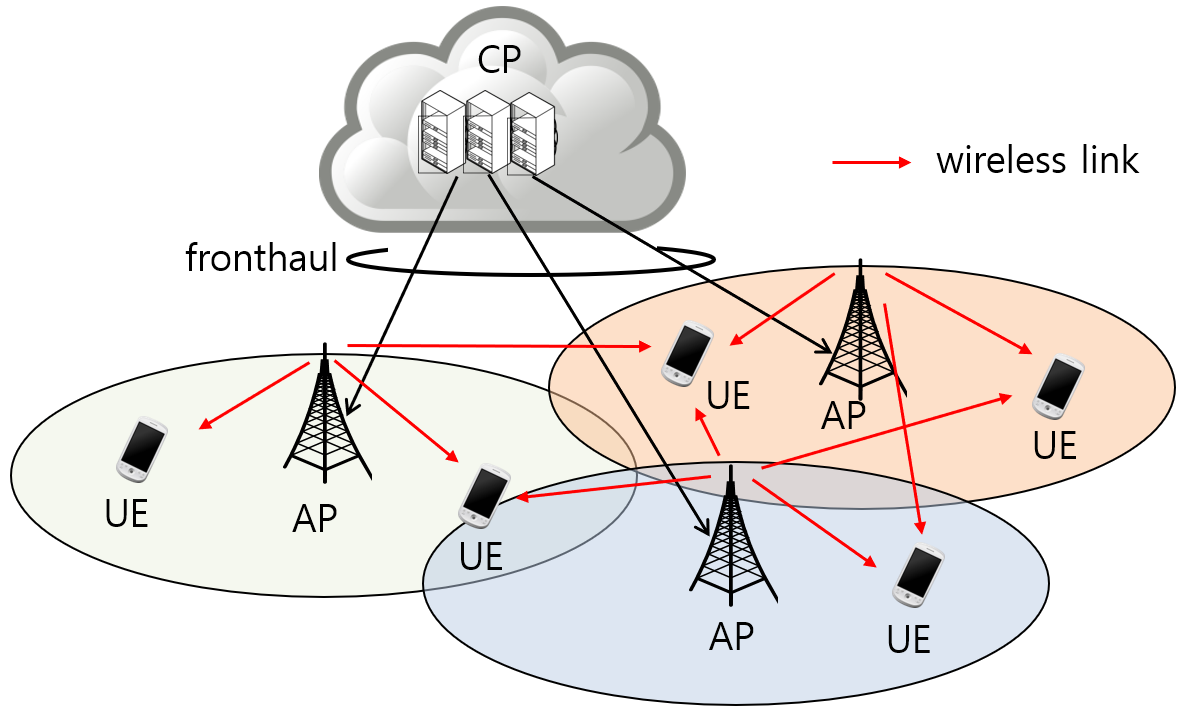
Figure 1: An example of cell-free MIMO system, in which a CP communicates with K=5K=5 UEs through M=3M=3 APs.

As shown in Fig. 1, we consider the downlink of a cell-free MIMO system in which KK single-antenna UEs are served by MM single-antenna APs controlled by a CP. Define the index sets for APs and UEs as ℳ={1,2,…,M}\mathcal{M}=\{1,2,\ldots,M\} and 𝒦={1,2,…,K}\mathcal{K}=\{1,2,\ldots,K\}, respectively. The discrete message intended for UE k∈𝒦k\in\mathcal{K} and its data rate in bps/Hz are denoted by WkW_{k} and RkR_{k}, respectively. The CP communicates with each AP i∈ℳi\in\mathcal{M} via a digital fronthaul link of capacity CfhC_{\text{fh}} bps/Hz.

The received signal of UE k∈𝒦k\in\mathcal{K} is written as

yk=𝐡kH​𝐱+nk,\displaystyle y_{k}=\mathbf{h}_{k}^{H}\mathbf{x}+n_{k}, (1)

where 𝐡k∈ℂM×1\mathbf{h}_{k}\in\mathbb{C}^{M\times 1} denotes the channel vector from all APs to UE kk, 𝐱∈ℂM×1\mathbf{x}\in\mathbb{C}^{M\times 1} is the signal vector transmitted by all APs, and nk∼𝒞​𝒩​(0,σ2)n_{k}\sim\mathcal{CN}(0,\sigma^{2}) indicates the additive noise at UE kk. The iith elements of 𝐡k\mathbf{h}_{k} and 𝐱\mathbf{x} are respectively denoted by hk,ih_{k,i} and xix_{i}. Each AP ii has a limited power budget PtxP_{\text{tx}}, imposing 𝔼⁡[|xi|2]≤Ptx\mathbb{E}[|x_{i}|^{2}]\leq P_{\text{tx}} for all i∈ℳi\in\mathcal{M}. The channel coefficients hk,ih_{k,i} are independent across the indices kk and ii due to the fact that the APs and UEs are distributed. Also, we assume Rayleigh fading channels hk,i∼𝒞​𝒩​(0,αk,i)h_{k,i}\sim\mathcal{CN}(0,\alpha_{k,i}), where 𝔼⁡[|hk,i|2]=αk,i\mathbb{E}[|h_{k,i}|^{2}]=\alpha_{k,i} stands for the path-loss between UE kk and AP ii.

We consider a time-division duplexing (TDD) system, in which the downlink CSI is obtained by uplink channel training process. Accordingly, the UEs send pilot signals on the uplink channel, and the APs transfer the received pilot signals to the CP which estimates global CSI based on the collected pilot signals. We denote an estimate of hk,ih_{k,i} by h^k,i\hat{h}_{k,i}, which is related to the true channel hk,ih_{k,i} as

hk,i=h^k,i+ek,i.\displaystyle h_{k,i}=\hat{h}_{k,i}+e_{k,i}. (2)

Here the difference ek,i=hk,i−h^k,ie_{k,i}=h_{k,i}-\hat{h}_{k,i} indicates the estimation error. If a linear minimum mean squared error (MMSE) estimator is employed at the CP, estimate h^k,i\hat{h}_{k,i} and error ek,ie_{k,i} are uncorrelated, and ek,ie_{k,i} follows a Gaussian distribution, i.e., ek,i∼𝒞​𝒩​(0,zk,i)e_{k,i}\sim\mathcal{CN}(0,z_{k,i}) [11, 12], where zk,i=𝔼⁡[|ek,i|2]z_{k,i}=\mathbb{E}[|e_{k,i}|^{2}] represents the estimation error power. Thus, we have αk,i=𝔼⁡[|h^k,i|2]+zk,i\alpha_{k,i}=\mathbb{E}[|\hat{h}_{k,i}|^{2}]+z_{k,i}.

Throughout the paper, we assume that the CP has knowledge of global estimated CSI 𝐡^={h^k,i}k∈𝒦,i∈ℳ\hat{\mathbf{h}}=\{\hat{h}_{k,i}\}_{k\in\mathcal{K},i\in\mathcal{M}} and of the estimation error powers 𝐳={zk,i}k∈𝒦,i∈ℳ\mathbf{z}=\{z_{k,i}\}_{k\in\mathcal{K},i\in\mathcal{M}}. Also, for fairness among the UEs, we focus on maximizing the minimum-rate Rmin=mink∈𝒦⁡RkR_{\min}=\min_{k\in\mathcal{K}}R_{k} of all UEs.

III Single-Layer Schemes: SDMA and NOMA

In this section, we discuss single-layer transmission schemes, in which the message WkW_{k} for each UE kk is encoded into a baseband data signal sk∼𝒞​𝒩​(0,1)s_{k}\sim\mathcal{CN}(0,1). Each signal sks_{k} is beamformed with a vector 𝐯k∈ℂM×1\mathbf{v}_{k}\in\mathbb{C}^{M\times 1}, and the beamforming output signals are quantized and compressed to bit streams which are delivered to the corresponding APs on fronthaul links. The transmitted signal vector 𝐱\mathbf{x} of APs, obtained by decompressing the fronthaul bit streams, is given as

𝐱=∑k∈𝒦𝐯k​sk+𝐪.\displaystyle\mathbf{x}=\sum_{k\in\mathcal{K}}\mathbf{v}_{k}s_{k}+\mathbf{q}. (3)

In (3), the vector 𝐪∼𝒞​𝒩​(𝟎,𝛀)\mathbf{q}\sim\mathcal{CN}(\mathbf{0},\boldsymbol{\Omega}) represents quantization distortion noise, which is uncorrelated with the beamformed signal 𝐱~=∑k∈𝒦𝐯k​sk\tilde{\mathbf{x}}=\sum_{k\in\mathcal{K}}\mathbf{v}_{k}s_{k}. We consider an independent quantization of the elements of 𝐱~=[x~1x~2⋯x~M]T\tilde{\mathbf{x}}=[\tilde{x}_{1}\,\tilde{x}_{2}\,\cdots\,\tilde{x}_{M}]^{T} so that we have 𝛀=diag​({ωi}i∈ℳ)\boldsymbol{\Omega}=\text{diag}(\{\omega_{i}\}_{i\in\mathcal{M}}) [13]. The beamforming vectors 𝐯={𝐯k}k∈𝒦\mathbf{v}=\{\mathbf{v}_{k}\}_{k\in\mathcal{K}} and the quantization noise powers 𝝎={ωi}i∈ℳ\boldsymbol{\omega}=\{\omega_{i}\}_{i\in\mathcal{M}} must satisfy the constraints

∑k∈𝒦|vk,i|2+ωi≤Ptx,i∈ℳ,\displaystyle\sum_{k\in\mathcal{K}}|v_{k,i}|^{2}+\omega_{i}\leq P_{\text{tx}},\,i\in\mathcal{M}, (4a)
ωi≥β​∑k∈𝒦|vk,i|2,i∈ℳ,\displaystyle\omega_{i}\geq\beta\sum_{k\in\mathcal{K}}|v_{k,i}|^{2},\,i\in\mathcal{M}, (4b)

where vk,iv_{k,i} denotes the iith element of 𝐯k\mathbf{v}_{k}, and β\beta is defined as β=1/(2Cfh−1)\beta=1/(2^{C_{\text{fh}}}-1). The constraint (4a) rewrites the power constraint 𝔼⁡[|xi|2]≤Ptx\mathbb{E}[|x_{i}|^{2}]\leq P_{\text{tx}}, and the constraint (4b) is imposed for successful decompression at APs and comes from the fronthaul capacity constraints I⁡(x~i,xi)≤CfhI(\tilde{x}_{i};x_{i})\leq C_{\text{fh}} [10, 13].

Each UE kk decodes its intended signal sks_{k} using the received signal yk=∑l∈𝒦𝐡kH​𝐯l​sl+𝐡kH​𝐪+zky_{k}=\sum_{l\in\mathcal{K}}\mathbf{h}_{k}^{H}\mathbf{v}_{l}s_{l}+\mathbf{h}_{k}^{H}\mathbf{q}+z_{k}. The single-layer schemes with single-user decoding (SUD) [3] and SIC decoding [4] are referred to as SDMA and NOMA, respectively [1]. We discuss these schemes in the following subsections.

III-A SDMA (Single-User Decoding)

In the SDMA scheme [1], UE kk decodes the data signal sks_{k} while treating the interference signals {sl}l∈𝒦∖{k}\{s_{l}\}_{l\in\mathcal{K}\setminus\{k\}} as noise. For given estimated CSI 𝐡^k\hat{\mathbf{h}}_{k}, the expected data rate RkR_{k} of UE kk is given as [11]

Rk=𝔼𝐞k​[log2⁡(1+γk)|𝐡^k],\displaystyle R_{k}=\mathbb{E}_{\mathbf{e}_{k}}\left[\log_{2}\left(1+\gamma_{k}\right)\Big|\hat{\mathbf{h}}_{k}\right], (5)

with the error vector 𝐞k=[ek,1ek,2⋯ek,M]T\mathbf{e}_{k}=[e_{k,1}\,e_{k,2}\,\cdots\,e_{k,M}]^{T} and the signal-to-interference-plus-noise ratio (SINR)

γk=𝐡^kH​𝐕k​𝐡^kσ2+𝐞kH​𝐕k​𝐞k+𝐡kH​(𝛀+𝐕𝒦∖{k})​𝐡k.\displaystyle\gamma_{k}=\frac{\hat{\mathbf{h}}_{k}^{H}\mathbf{V}_{k}\hat{\mathbf{h}}_{k}}{\sigma^{2}+\mathbf{e}_{k}^{H}\mathbf{V}_{k}\mathbf{e}_{k}+\mathbf{h}_{k}^{H}\left(\boldsymbol{\Omega}+\mathbf{V}_{\mathcal{K}\setminus\{k\}}\right)\mathbf{h}_{k}}. (6)

In (6), we have defined the notations 𝐕k=𝐯k​𝐯kH\mathbf{V}_{k}=\mathbf{v}_{k}\mathbf{v}_{k}^{H} and 𝐕𝒮=∑m∈𝒮𝐕m\mathbf{V}_{\mathcal{S}}=\sum_{m\in\mathcal{S}}\mathbf{V}_{m}. The second term 𝐞kH​𝐕k​𝐞k\mathbf{e}_{k}^{H}\mathbf{V}_{k}\mathbf{e}_{k} in the denominator of (6) indicates the self-interference signal power caused by erroneous CSI.

As in [11, 12], we use Jensen’s inequality to obtain a closed-form expression for (6), which serves as a lower bound on the rate (5), i.e.,

Rk≥fk​(𝐕,𝝎)=log2⁡(1+γ~k),\displaystyle R_{k}\geq f_{k}(\mathbf{V},\boldsymbol{\omega})=\log_{2}\left(1+\tilde{\gamma}_{k}\right), (7)

where γ~k\tilde{\gamma}_{k} is defined as

γ~k\displaystyle\tilde{\gamma}_{k} =𝐡^kH​𝐕k​𝐡^kσ2+𝔼𝐞k​[𝐞kH​𝐕k​𝐞k]+𝔼𝐞k​[𝐡kH​(𝛀+𝐕𝒦∖{k})​𝐡k|𝐡^k]\displaystyle=\frac{\hat{\mathbf{h}}_{k}^{H}\mathbf{V}_{k}\hat{\mathbf{h}}_{k}}{\sigma^{2}+\mathbb{E}_{\mathbf{e}_{k}}\big[\mathbf{e}_{k}^{H}\mathbf{V}_{k}\mathbf{e}_{k}\big]+\mathbb{E}_{\mathbf{e}_{k}}\big[\mathbf{h}_{k}^{H}\left(\boldsymbol{\Omega}+\mathbf{V}_{\mathcal{K}\setminus\{k\}}\right)\mathbf{h}_{k}\big|\hat{\mathbf{h}}_{k}\big]}
=𝐡^kH​𝐕k​𝐡^kσ2+𝐳kH​(𝛀+𝐕d,𝒦)​𝐳k+𝐡^kH​(𝛀+𝐕𝒦∖{k})​𝐡^k,\displaystyle=\frac{\hat{\mathbf{h}}_{k}^{H}\mathbf{V}_{k}\hat{\mathbf{h}}_{k}}{\sigma^{2}+\mathbf{z}_{k}^{H}(\boldsymbol{\Omega}+\mathbf{V}_{d,\mathcal{K}})\mathbf{z}_{k}+\hat{\mathbf{h}}_{k}^{H}\left(\boldsymbol{\Omega}+\mathbf{V}_{\mathcal{K}\setminus\{k\}}\right)\hat{\mathbf{h}}_{k}}, (8)

with the notation 𝐳k=[zk,11/2zk,21/2⋯,zk,M1/2]T\mathbf{z}_{k}=[z_{k,1}^{1/2}\,z_{k,2}^{1/2}\,\cdots,z_{k,M}^{1/2}]^{T} and the matrix 𝐕d,𝒮\mathbf{V}_{d,\mathcal{S}} obtained by replacing all the off-diagonal elements of 𝐕𝒮\mathbf{V}_{\mathcal{S}} with zeros.

The optimization of beamforming 𝐕\mathbf{V} and fronthaul quantization noise powers 𝝎\boldsymbol{\omega} of SDMA for minimum-rate maximization can be formulated as

max.𝐕,𝝎\displaystyle\underset{\mathbf{V},\boldsymbol{\omega}}{\mathrm{max.}}\,\,\, mink∈𝒦⁡fk​(𝐕,𝝎)\displaystyle\min_{k\in\mathcal{K}}f_{k}(\mathbf{V},\boldsymbol{\omega}) (9a)
s.t.\displaystyle\mathrm{s.t.}\,\,\,\,\,\, 𝐞iH​𝐕𝒦​𝐞i+ωi≤Ptx,i∈ℳ\displaystyle\mathbf{e}_{i}^{H}\mathbf{V}_{\mathcal{K}}\mathbf{e}_{i}+\omega_{i}\leq P_{\text{tx}},\,i\in\mathcal{M} (9b)
ωi≥β​𝐞iH​𝐕𝒦​𝐞i,i∈ℳ\displaystyle\omega_{i}\geq\beta\mathbf{e}_{i}^{H}\mathbf{V}_{\mathcal{K}}\mathbf{e}_{i},\,i\in\mathcal{M} (9c)
rank​(𝐕k)≤1,k∈𝒦,\displaystyle\text{rank}(\mathbf{V}_{k})\leq 1,\,k\in\mathcal{K}, (9d)

where 𝐞i∈ℂM×1\mathbf{e}_{i}\in\mathbb{C}^{M\times 1} is a vector whose elements are zeros except for the iith element equal to 1. The problem (9) can be converted to a difference-of-convex (DC) problem by rewriting the function fk​(𝐕,𝝎)f_{k}(\mathbf{\mathbf{V}},\boldsymbol{\omega}) in (7) as

log2⁡(σ2+𝐳kH​(𝛀+𝐕d,𝒦)​𝐳k+𝐡^kH​(𝛀+𝐕𝒦)​𝐡^k)\displaystyle\log_{2}\left(\sigma^{2}+\mathbf{z}_{k}^{H}\left(\boldsymbol{\Omega}+\mathbf{V}_{d,\mathcal{K}}\right)\mathbf{z}_{k}+\hat{\mathbf{h}}_{k}^{H}\left(\boldsymbol{\Omega}+\mathbf{V}_{\mathcal{K}}\right)\hat{\mathbf{h}}_{k}\right)
−log2⁡(σ2+𝐳kH​(𝛀+𝐕d,𝒦)​𝐳k+𝐡^kH​(𝛀+𝐕𝒦∖{k})​𝐡^k),\displaystyle-\log_{2}\left(\sigma^{2}+\mathbf{z}_{k}^{H}\left(\boldsymbol{\Omega}+\mathbf{V}_{d,\mathcal{K}}\right)\mathbf{z}_{k}+\hat{\mathbf{h}}_{k}^{H}\left(\boldsymbol{\Omega}+\mathbf{V}_{\mathcal{K}\setminus\{k\}}\right)\hat{\mathbf{h}}_{k}\right),

and relaxing the rank constraint (9d). Thus, we can find a locally optimal solution by adopting the MM approach [10] of the modified problem, and a feasible rank-1 solution can be found by a projection process.

III-B NOMA (SIC Decoding)

In the standard downlink NOMA scheme [4], the UEs perform SIC decoding with a given decoding order sπ⁡(1)→sπ⁡(2)→…→sπ⁡(K)s_{\pi(1)}\rightarrow s_{\pi(2)}\rightarrow\ldots\rightarrow s_{\pi(K)}, until their intended signals are obtained. With this approach, each data signal sπ⁡(k)s_{\pi(k)} should be successfully decoded at the intended UE π⁡(k)\pi(k) as well as the UEs π⁡(k+1),π⁡(k+2),…,π⁡(K)\pi(k+1),\pi(k+2),\ldots,\pi(K) which decode it before their intended signals. Thus, the expected data rate Rπ⁡(k)R_{\pi(k)} of UE π⁡(k)\pi(k) under NOMA is given as

Rπ⁡(k)=minl∈[k:K]𝔼𝐞π⁡(l)[log2(1+γl,k)|𝐡^π⁡(l)],\displaystyle R_{\pi(k)}=\min_{l\in[k:K]}\mathbb{E}_{\mathbf{e}_{\pi(l)}}\left[\log_{2}\left(1+\gamma_{l,k}\right)\Big|\hat{\mathbf{h}}_{\pi(l)}\right], (10)

where [k:K]={k,k+1,…,K}[k:K]=\{k,k+1,\ldots,K\} and

γl,k=𝐡^π⁡(l)H​𝐕π⁡(k)​𝐡^π⁡(l)σ2+𝐞π⁡(l)H​𝐕π⁡(k)​𝐞π⁡(l)+𝐡π⁡(l)H​(𝛀+𝐕{π⁡(m)}m=k+1K)​𝐡π⁡(l).\displaystyle\gamma_{l,k}=\frac{\hat{\mathbf{h}}_{\pi(l)}^{H}\mathbf{V}_{\pi(k)}\hat{\mathbf{h}}_{\pi(l)}}{\sigma^{2}+\mathbf{e}_{\pi(l)}^{H}\mathbf{V}_{\pi(k)}\mathbf{e}_{\pi(l)}+\mathbf{h}_{\pi(l)}^{H}\left(\boldsymbol{\Omega}+\mathbf{V}_{\{\pi(m)\}_{m=k+1}^{K}}\right)\mathbf{h}_{\pi(l)}}. (11)

Similar to SDMA, we replace each expected rate 𝔼𝐞π⁡(l)​[log2⁡(1+γl,k)|𝐡^π⁡(l)]\mathbb{E}_{\mathbf{e}_{\pi(l)}}[\log_{2}(1+\gamma_{l,k})\big|\hat{\mathbf{h}}_{\pi(l)}] with the closed-form lower bound expression

fl,k​(𝐕,𝝎)=log2⁡(1+𝐡^π⁡(l)H​𝐕π⁡(k)​𝐡^π⁡(l)σ2+IN,l,k),\displaystyle f_{l,k}(\mathbf{V},\boldsymbol{\omega})=\log_{2}\left(1+\frac{\hat{\mathbf{h}}_{\pi(l)}^{H}\mathbf{V}_{\pi(k)}\hat{\mathbf{h}}_{\pi(l)}}{\sigma^{2}+I_{N,l,k}}\right), (12)

where

IN,l,k\displaystyle I_{N,l,k} =𝔼𝐞π⁡(l)​[𝐞π⁡(l)H​𝐕π⁡(k)​𝐞π⁡(l)]+𝔼𝐞π⁡(l)​[𝐡π⁡(l)H​(𝛀+𝐕{π⁡(m)}m=k+1K)​𝐡π⁡(l)|𝐡^π⁡(l)]\displaystyle=\mathbb{E}_{\mathbf{e}_{\pi(l)}}\left[\mathbf{e}_{\pi(l)}^{H}\mathbf{V}_{\pi(k)}\mathbf{e}_{\pi(l)}\right]+\mathbb{E}_{\mathbf{e}_{\pi(l)}}\left[\mathbf{h}_{\pi(l)}^{H}\left(\boldsymbol{\Omega}+\mathbf{V}_{\{\pi(m)\}_{m=k+1}^{K}}\right)\mathbf{h}_{\pi(l)}\Big|\hat{\mathbf{h}}_{\pi(l)}\right]
=𝐳π⁡(l)H​(𝛀+𝐕d,𝒦)​𝐳π⁡(l)+𝐡^π⁡(l)H​(𝛀+𝐕{π⁡(m)}m=k+1K)​𝐡^π⁡(l).\displaystyle=\mathbf{z}_{\pi(l)}^{H}\left(\boldsymbol{\Omega}+\mathbf{V}_{d,\mathcal{K}}\right)\mathbf{z}_{\pi(l)}+\hat{\mathbf{h}}_{\pi(l)}^{H}\left(\boldsymbol{\Omega}+\mathbf{V}_{\{\pi(m)\}_{m=k+1}^{K}}\right)\hat{\mathbf{h}}_{\pi(l)}. (13)

We can state the problem of minimum-rate maximization for NOMA scheme as

max.𝐕,𝝎,𝐑\displaystyle\underset{\mathbf{V},\boldsymbol{\omega},\mathbf{R}}{\mathrm{max.}}\,\,\, mink∈𝒦⁡Rk\displaystyle\min_{k\in\mathcal{K}}R_{k} (14a)
s.t.\displaystyle\mathrm{s.t.}\,\,\,\,\,\, Rπ⁡(k)≤fl,k(𝐕,𝝎),k∈𝒦,l∈[k:K]\displaystyle R_{\pi(k)}\leq f_{l,k}(\mathbf{V},\boldsymbol{\omega}),\,k\in\mathcal{K},l\in[k:K] (14b)
𝐞iH​𝐕𝒦​𝐞i+ωi≤Ptx,i∈ℳ\displaystyle\mathbf{e}_{i}^{H}\mathbf{V}_{\mathcal{K}}\mathbf{e}_{i}+\omega_{i}\leq P_{\text{tx}},\,i\in\mathcal{M} (14c)
ωi≥β​𝐞iH​𝐕𝒦​𝐞i,i∈ℳ\displaystyle\omega_{i}\geq\beta\mathbf{e}_{i}^{H}\mathbf{V}_{\mathcal{K}}\mathbf{e}_{i},\,i\in\mathcal{M} (14d)
rank​(𝐕k)≤1,k∈𝒦,\displaystyle\text{rank}(\mathbf{V}_{k})\leq 1,\,k\in\mathcal{K}, (14e)

with 𝐑={Rk}k∈𝒦\mathbf{R}=\{R_{k}\}_{k\in\mathcal{K}}. Similar to (9), we can obtain a problem of DC form by rewriting the function fl,k​(𝐯,𝝎)f_{l,k}(\mathbf{v},\boldsymbol{\omega}) in (12) as

log2⁡(σ2+IN,l,k+𝐡^π⁡(l)H​𝐕π⁡(k)​𝐡^π⁡(l))−log2⁡(σ2+IN,l,k),\displaystyle\log_{2}\left(\sigma^{2}+I_{N,l,k}+\hat{\mathbf{h}}_{\pi(l)}^{H}\mathbf{V}_{\pi(k)}\hat{\mathbf{h}}_{\pi(l)}\right)-\log_{2}\left(\sigma^{2}+I_{N,l,k}\right),

and removing the rank constraint (14e).

IV Rate-Splitting Multiple Access

To describe a general RSMA scheme, we denote the number of common signals by LL and define the set of common signals’ indices as ℒ={1,2,…,L}\mathcal{L}=\{1,2,\ldots,L\}. We assume that the llth common signal is decoded by the UEs in subset 𝒮l⊆𝒦\mathcal{S}_{l}\subseteq\mathcal{K}. To remove redundancy in the design, the subsets 𝒮1,𝒮2,…,𝒮L\mathcal{S}_{1},\mathcal{S}_{2},\ldots,\mathcal{S}_{L} satisfy the conditions 𝒮l1≠𝒮l2\mathcal{S}_{l_{1}}\neq\mathcal{S}_{l_{2}} for all l1≠l2∈ℒl_{1}\neq l_{2}\in\mathcal{L}. Also, to differentiate from private signals each of which is decoded by a single UE, we have |𝒮l|≥2|\mathcal{S}_{l}|\geq 2, l∈ℒl\in\mathcal{L}. For given 𝒮1,𝒮2,…,𝒮L\mathcal{S}_{1},\mathcal{S}_{2},\ldots,\mathcal{S}_{L}, we can figure out the set ℒk\mathcal{L}_{k} of common signals’ indices that contain UE kk, i.e., ℒk={l∈ℒ|k∈𝒮l}\mathcal{L}_{k}=\{l\in\mathcal{L}|k\in\mathcal{S}_{l}\}.

IV-A Overall Operation and Beamforming Optimization

In the RSMA scheme, the message WkW_{k} for UE kk is split into Lk+1L_{k}+1 messages, i.e., a private message Wp,kW_{p,k} and LkL_{k} common messages {Wc,k,l}l∈ℒk\{W_{c,k,l}\}_{l\in\mathcal{L}_{k}}, where Lk=|ℒk|L_{k}=|\mathcal{L}_{k}|. The private message Wp,kW_{p,k} is decoded only by UE kk, and the common message Wc,k,lW_{c,k,l} is decoded by all UEs in the set ℒk\mathcal{L}_{k}. Denoting the rates of Wp,kW_{p,k} and Wc,k,lW_{c,k,l} by Rp,kR_{p,k} and Rc,k,lR_{c,k,l}, respectively, we can write Rk=Rp,k+∑l∈ℒkRc,k,lR_{k}=R_{p,k}+\sum_{l\in\mathcal{L}_{k}}R_{c,k,l}.

The private messages Wp,kW_{p,k}, k∈𝒦k\in\mathcal{K}, are separately encoded, so the resulting private symbols sp,k∼𝒞​𝒩​(0,1)s_{p,k}\sim\mathcal{CN}(0,1) with k∈𝒦k\in\mathcal{K} are independent. The common messages Wc,k,lW_{c,k,l}, k∈𝒮lk\in\mathcal{S}_{l}, associated with the llth subset 𝒮l\mathcal{S}_{l} are concatenated and encoded to a single common signal sc,l∼𝒞​𝒩​(0,1)s_{c,l}\sim\mathcal{CN}(0,1). Accordingly, the common signal sc,ls_{c,l} is decoded by all UEs in 𝒮l\mathcal{S}_{l}, and each UE k∈𝒮lk\in\mathcal{S}_{l} can extract its common message Wc,k,lW_{c,k,l} from sc,ls_{c,l}.

Denoting the beamforming vectors for signals sp,ks_{p,k} and sc,ls_{c,l} by 𝐯p,k∈ℂM×1\mathbf{v}_{p,k}\in\mathbb{C}^{M\times 1} and 𝐯c,l∈ℂM×1\mathbf{v}_{c,l}\in\mathbb{C}^{M\times 1}, respectively, the transmitted signal vector 𝐱\mathbf{x} of APs is given as

𝐱=∑k∈𝒦𝐯p,k​sp,k+∑l∈ℒ𝐯c,l​sc,l+𝐪.\displaystyle\mathbf{x}=\sum_{k\in\mathcal{K}}\mathbf{v}_{p,k}s_{p,k}+\sum_{l\in\mathcal{L}}\mathbf{v}_{c,l}s_{c,l}+\mathbf{q}. (15)

If we denote the iith elements of 𝐯p,k\mathbf{v}_{p,k} and 𝐯c,l\mathbf{v}_{c,l} by vp,k,iv_{p,k,i} and vc,l,iv_{c,l,i}, the power and fronthaul capacity constraints at AP ii can be written as

∑k∈𝒦|vp,k,i|2+∑l∈ℒ|vc,l,i|2+ωi≤Ptx,i∈ℳ.\displaystyle\sum_{k\in\mathcal{K}}|v_{p,k,i}|^{2}+\sum_{l\in\mathcal{L}}|v_{c,l,i}|^{2}+\omega_{i}\leq P_{\text{tx}},\,i\in\mathcal{M}. (16a)
ωi≥β⁡(∑k∈𝒦|vp,k,i|2+∑l∈ℒ|vc,l,i|2),i∈ℳ.\displaystyle\omega_{i}\geq\beta\left(\sum_{k\in\mathcal{K}}|v_{p,k,i}|^{2}+\sum_{l\in\mathcal{L}}|v_{c,l,i}|^{2}\right),\,i\in\mathcal{M}. (16b)

UE kk decodes the messages Wp,kW_{p,k} and {Wc,k,l}l∈ℒk\{W_{c,k,l}\}_{l\in\mathcal{L}_{k}}, which were split from the original message WkW_{k}, based on the received signal yky_{k}. This means that UE kk should decode the corresponding data signals sp,ks_{p,k} and {sc,l}l∈ℒk\{s_{c,l}\}_{l\in\mathcal{L}_{k}}. We assume that the SIC decoding is performed with the order sc,πk​(1)→sc,πk​(2)→…→sc,πk​(Lk)→sp,ks_{c,\pi_{k}(1)}\rightarrow s_{c,\pi_{k}(2)}\rightarrow\ldots\rightarrow s_{c,\pi_{k}(L_{k})}\rightarrow s_{p,k}. The decoding order πk\pi_{k} is chosen guaranteeing that |𝒮πk​(l1)|≥|𝒮πk​(l2)||\mathcal{S}_{\pi_{k}(l_{1})}|\geq|\mathcal{S}_{\pi_{k}(l_{2})}| for all l1<l2∈{1,2,…,Lk}l_{1}<l_{2}\in\{1,2,\ldots,L_{k}\} [1, 8].

The expected data rates {Rp,k}k∈𝒦\{R_{p,k}\}_{k\in\mathcal{K}} and {Rc,k,l}k∈𝒦,l∈ℒk\{R_{c,k,l}\}_{k\in\mathcal{K},l\in\mathcal{L}_{k}} are achievable if they satisfy the conditions

∑k∈𝒮lRc,k,l≤mink∈𝒮l⁡𝔼𝐞k​[log2⁡(1+γc,k,l)|𝐡^k],l∈ℒ,\displaystyle\sum\nolimits_{k\in\mathcal{S}_{l}}\!\!R_{c,k,l}\!\leq\!\min_{k\in\mathcal{S}_{l}}\mathbb{E}_{\mathbf{e}_{k}}\!\!\left[\log_{2}\!\left(1+\gamma_{c,k,l}\right)\!\Big|\hat{\mathbf{h}}_{k}\right]\!,l\in\mathcal{L}, (17a)
Rp,k≤𝔼𝐞k​[log2⁡(1+γp,k)|𝐡^k],k∈𝒦,\displaystyle R_{p,k}\leq\mathbb{E}_{\mathbf{e}_{k}}\left[\log_{2}\left(1+\gamma_{p,k}\right)\Big|\hat{\mathbf{h}}_{k}\right],\,\,k\in\mathcal{K}, (17b)

where

γc,k,l=𝐡^kH​𝐕c,l​𝐡^kσ2+𝐞kH​𝐕c,l​𝐞k+𝐡kH​(𝛀+𝐕p,𝒦+𝐕c,ℒ∖ℒk+𝐕c,𝒬k,l)​𝐡k\displaystyle\gamma_{c,k,l}=\frac{\hat{\mathbf{h}}_{k}^{H}\mathbf{V}_{c,l}\hat{\mathbf{h}}_{k}}{\sigma^{2}+\mathbf{e}_{k}^{H}\mathbf{V}_{c,l}\mathbf{e}_{k}+\mathbf{h}_{k}^{H}\big(\boldsymbol{\Omega}+\mathbf{V}_{p,\mathcal{K}}+\mathbf{V}_{c,\mathcal{L}\setminus\mathcal{L}_{k}}+\mathbf{V}_{c,\mathcal{Q}_{k,l}}\big)\mathbf{h}_{k}} (18a)
γp,k=𝐡^kH​𝐕p,k​𝐡^k𝐞kH​𝐕p,k​𝐞k+𝐡kH​(𝛀+𝐕p,𝒦∖{k}+𝐕c,ℒ∖ℒk)​𝐡k,\displaystyle\gamma_{p,k}=\frac{\hat{\mathbf{h}}_{k}^{H}\mathbf{V}_{p,k}\hat{\mathbf{h}}_{k}}{\mathbf{e}_{k}^{H}\mathbf{V}_{p,k}\mathbf{e}_{k}+\mathbf{h}_{k}^{H}\big(\boldsymbol{\Omega}+\mathbf{V}_{p,\mathcal{K}\setminus\{k\}}+\mathbf{V}_{c,\mathcal{L}\setminus\mathcal{L}_{k}}\big)\mathbf{h}_{k}}, (18b)

with 𝒬k,l={πk​(q)}q=πk−1​(l)+1Lk\mathcal{Q}_{k,l}=\{\pi_{k}(q)\}_{q=\pi_{k}^{-1}(l)+1}^{L_{k}}.

Similar to Sec. III, we consider lower bound expressions 𝔼𝐞k​[log2⁡(1+γc,k,l)|𝐡^k]≥fc,l​(𝐕,𝝎)\mathbb{E}_{\mathbf{e}_{k}}[\log_{2}(1+\gamma_{c,k,l})\big|\hat{\mathbf{h}}_{k}]\geq f_{c,l}(\mathbf{V},\boldsymbol{\omega}) and 𝔼𝐞k​[log2⁡(1+γp,k)|𝐡^k]≥fp,k​(𝐕,𝝎)\mathbb{E}_{\mathbf{e}_{k}}[\log_{2}(1+\gamma_{p,k})\big|\hat{\mathbf{h}}_{k}]\geq f_{p,k}(\mathbf{V},\boldsymbol{\omega}), where we define the functions

fc,k,l​(𝐕,𝝎)=log2⁡(1+𝐡^kH​𝐕c,l​𝐡^kσ2+Ic,k,l),\displaystyle f_{c,k,l}(\mathbf{V},\boldsymbol{\omega})=\log_{2}\left(1+\frac{\hat{\mathbf{h}}_{k}^{H}\mathbf{V}_{c,l}\hat{\mathbf{h}}_{k}}{\sigma^{2}+I_{c,k,l}}\right), (19a)
fp,k​(𝐕,𝝎)=log2⁡(1+𝐡^kH​𝐕p,k​𝐡^kσ2+Ip,k).\displaystyle f_{p,k}(\mathbf{V},\boldsymbol{\omega})=\log_{2}\left(1+\frac{\hat{\mathbf{h}}_{k}^{H}\mathbf{V}_{p,k}\hat{\mathbf{h}}_{k}}{\sigma^{2}+I_{p,k}}\right). (19b)

with

Ic,k,l\displaystyle I_{c,k,l} =𝐳kH​(𝛀+𝐕d,c,ℒ+𝐕d,p,𝒦)​𝐳k+𝐡^kH​(𝛀+𝐕p,𝒦+𝐕c,ℒ∖ℒk+𝐕c,𝒬k,l)​𝐡^k,\displaystyle=\mathbf{z}_{k}^{H}\left(\boldsymbol{\Omega}+\mathbf{V}_{d,c,\mathcal{L}}+\mathbf{V}_{d,p,\mathcal{K}}\right)\mathbf{z}_{k}+\hat{\mathbf{h}}_{k}^{H}\left(\boldsymbol{\Omega}+\mathbf{V}_{p,\mathcal{K}}+\mathbf{V}_{c,\mathcal{L}\setminus\mathcal{L}_{k}}+\mathbf{V}_{c,\mathcal{Q}_{k,l}}\right)\hat{\mathbf{h}}_{k}, (20a)
Ip,k\displaystyle I_{p,k} =𝐳kH​(𝛀+𝐕d,c,ℒ+𝐕d,p,𝒦)​𝐳k+𝐡^kH​(𝛀+𝐕p,𝒦∖{k}+𝐕c,ℒ∖ℒk)​𝐡^k.\displaystyle=\mathbf{z}_{k}^{H}\left(\boldsymbol{\Omega}+\mathbf{V}_{d,c,\mathcal{L}}+\mathbf{V}_{d,p,\mathcal{K}}\right)\mathbf{z}_{k}+\hat{\mathbf{h}}_{k}^{H}\left(\boldsymbol{\Omega}+\mathbf{V}_{p,\mathcal{K}\setminus\{k\}}+\mathbf{V}_{c,\mathcal{L}\setminus\mathcal{L}_{k}}\right)\hat{\mathbf{h}}_{k}. (20b)

Unlike Sec. III, 𝐕\mathbf{V} denotes 𝐕={𝐕p,k}k∈𝒦∪{𝐕c,l}l∈ℒ\mathbf{V}=\{\mathbf{V}_{p,k}\}_{k\in\mathcal{K}}\cup\{\mathbf{V}_{c,l}\}_{l\in\mathcal{L}}.

The minimum-rate maximization for the RSMA scheme is stated as

max.𝐕,𝝎,𝐑\displaystyle\underset{\mathbf{V},\boldsymbol{\omega},\mathbf{R}}{\mathrm{max.}}\,\,\, mink∈𝒦⁡(Rp,k+∑l∈ℒkRc,k,l)\displaystyle\min_{k\in\mathcal{K}}\left(R_{p,k}+\sum_{l\in\mathcal{L}_{k}}R_{c,k,l}\right)\, (21a)
s.t.\displaystyle\mathrm{s.t.}\,\,\,\,\,\, ∑k∈𝒮lRc,k,l≤fc,k′,l​(𝐕,𝝎),l∈ℒ,k′∈𝒮l\displaystyle\sum_{k\in\mathcal{S}_{l}}R_{c,k,l}\leq f_{c,k^{\prime},l}(\mathbf{V},\boldsymbol{\omega}),\,l\in\mathcal{L},k^{\prime}\in\mathcal{S}_{l} (21b)
Rp,k≤fp,k​(𝐕,𝝎),k∈𝒦\displaystyle R_{p,k}\leq f_{p,k}(\mathbf{V},\boldsymbol{\omega}),\,k\in\mathcal{K} (21c)
𝐞iH​(𝐕c,ℒ+𝐕p,𝒦)​𝐞i+ωi≤Ptx,i∈ℳ\displaystyle\mathbf{e}_{i}^{H}\left(\mathbf{V}_{c,\mathcal{L}}+\mathbf{V}_{p,\mathcal{K}}\right)\mathbf{e}_{i}+\omega_{i}\leq P_{\text{tx}},\,i\in\mathcal{M} (21d)
ωi≥β​𝐞iH​(𝐕c,ℒ+𝐕p,𝒦)​𝐞i,i∈ℳ\displaystyle\omega_{i}\geq\beta\mathbf{e}_{i}^{H}\left(\mathbf{V}_{c,\mathcal{L}}+\mathbf{V}_{p,\mathcal{K}}\right)\mathbf{e}_{i},\,i\in\mathcal{M} (21e)
rank​(𝐕c,l)≤1,rank​(𝐕p,k)≤1,l∈ℒ,k∈𝒦,\displaystyle\text{rank}(\mathbf{V}_{c,l})\!\leq\!1,\text{rank}(\mathbf{V}_{p,k})\!\leq\!1,\,l\in\mathcal{L},k\in\mathcal{K}, (21f)

with the notations 𝐑={Rp,k}k∈𝒦∪{Rc,k,l}k∈𝒦,l∈ℒk\mathbf{R}=\{R_{p,k}\}_{k\in\mathcal{K}}\cup\{R_{c,k,l}\}_{k\in\mathcal{K},l\in\mathcal{L}_{k}}, 𝐕c,𝒮=∑l∈𝒮𝐕c,l\mathbf{V}_{c,\mathcal{S}}=\sum_{l\in\mathcal{S}}\mathbf{V}_{c,l}, and 𝐕p,𝒮=∑k∈𝒮𝐕p,k\mathbf{V}_{p,\mathcal{S}}=\sum_{k\in\mathcal{S}}\mathbf{V}_{p,k}. We can convert the problem (21) into a DC form by rewriting the functions fc,k′,l​(𝐕,𝝎)f_{c,k^{\prime},l}(\mathbf{V},\boldsymbol{\omega}) and fp,k​(𝐕,𝝎)f_{p,k}(\mathbf{V},\boldsymbol{\omega}) in (21b) and (21c) as log2⁡(σ2+Ic,k′,l+𝐡^k′H​𝐕c,l​𝐡^k′)−log2⁡(σ2+Ic,k′,l)\log_{2}(\sigma^{2}+I_{c,k^{\prime},l}+\hat{\mathbf{h}}_{k^{\prime}}^{H}\mathbf{V}_{c,l}\hat{\mathbf{h}}_{k^{\prime}})-\log_{2}(\sigma^{2}+I_{c,k^{\prime},l}) and log2⁡(σ2+Ip,k+𝐡^kH​𝐕p,k​𝐡^k)−log2⁡(σ2+Ip,k)\log_{2}(\sigma^{2}+I_{p,k}+\hat{\mathbf{h}}_{k}^{H}\mathbf{V}_{p,k}\hat{\mathbf{h}}_{k})-\log_{2}(\sigma^{2}+I_{p,k}), respectively. Thus, a locally optimal solution of the problem obtained by removing the rank constraints in (21f) can be found by an MM-based iterative algorithm [10]. Accordingly, at each iteration, the solution is updated to a better point by solving the convex problem obtained by convexifying the non-convex constraints (21b) and (21c). The detailed algorithm procedure is described in Algorithm 1, where

f~c,k′,l​(𝐕,𝝎,𝐕[t−1],𝝎[t−1])\displaystyle\tilde{f}_{c,k^{\prime},l}(\mathbf{V},\boldsymbol{\omega},\mathbf{V}^{[t-1]},\boldsymbol{\omega}^{[t-1]}) =log2⁡(σ2+Ic,k′,l+𝐡^k′H​𝐕c,l​𝐡^k′)\displaystyle=\log_{2}\left(\sigma^{2}+I_{c,k^{\prime},l}+\hat{\mathbf{h}}_{k^{\prime}}^{H}\mathbf{V}_{c,l}\hat{\mathbf{h}}_{k^{\prime}}\right)
−log2⁡(σ2+Ic,k′,l[t−1])−1ln⁡2​Ic,k′,l−Ic,k′,l[t−1]σ2+Ic,k′,l[t−1],\displaystyle-\log_{2}\left(\sigma^{2}+I_{c,k^{\prime},l}^{[t-1]}\right)-\frac{1}{\ln 2}\frac{I_{c,k^{\prime},l}-I_{c,k^{\prime},l}^{[t-1]}}{\sigma^{2}+I_{c,k^{\prime},l}^{[t-1]}}, (22a)
f~p,k​(𝐕,𝝎,𝐕[t−1],𝝎[t−1])\displaystyle\tilde{f}_{p,k}(\mathbf{V},\boldsymbol{\omega},\mathbf{V}^{[t-1]},\boldsymbol{\omega}^{[t-1]}) =log2⁡(σ2+Ip,k+𝐡^kH​𝐕p,k​𝐡^k)\displaystyle=\log_{2}\left(\sigma^{2}+I_{p,k}+\hat{\mathbf{h}}_{k}^{H}\mathbf{V}_{p,k}\hat{\mathbf{h}}_{k}\right)
−log2⁡(σ2+Ip,k[t−1])−1ln⁡2​Ip,k−Ip,k[t−1]σ2+Ip,k[t−1].\displaystyle-\log_{2}\left(\sigma^{2}+I_{p,k}^{[t-1]}\right)-\frac{1}{\ln 2}\frac{I_{p,k}-I_{p,k}^{[t-1]}}{\sigma^{2}+I_{p,k}^{[t-1]}}. (22b)

After Algorithm 1 is completed, feasible beamforming vectors 𝐯c,l\mathbf{v}_{c,l} and 𝐯p,k\mathbf{v}_{p,k} can be obtained from the quadratic matrices 𝐕c,l\mathbf{V}_{c,l} and 𝐕p,k\mathbf{V}_{p,k} by a projection process. For example, we obtain 𝐯c,l\mathbf{v}_{c,l} as 𝐯c,l←𝐮⁡(𝐕c,l)​λ1/2​(𝐕c,l)\mathbf{v}_{c,l}\leftarrow\mathbf{u}(\mathbf{V}_{c,l})\lambda^{1/2}(\mathbf{V}_{c,l}), where 𝐮1​(⋅)\mathbf{u}_{1}(\cdot) and λ1​(⋅)\lambda_{1}(\cdot) take the principal eigenvector and eigenvalue of the input square matrix.

Algorithm 1 MM based algorithm for problem (21)

1 Initialize

2 Set 𝐕[1]\mathbf{V}^{[1]} such that maxi∈ℳ⁡𝐞iH​𝐕𝒦[1]​𝐞i=11+β​Ptx\max_{i\in\mathcal{M}}\mathbf{e}_{i}^{H}\mathbf{V}_{\mathcal{K}}^{[1]}\mathbf{e}_{i}=\frac{1}{1+\beta}P_{\text{tx}};

3 Set ωi[1]←β1+β​𝐞iH​𝐕𝒦[1]​𝐞i\omega_{i}^{[1]}\leftarrow\frac{\beta}{1+\beta}\mathbf{e}_{i}^{H}\mathbf{V}_{\mathcal{K}}^{[1]}\mathbf{e}_{i}, i∈ℳi\in\mathcal{M};

4 Set t←1t\leftarrow 1;

5 repeat

6 Update t←t+1t\leftarrow t+1;

7 Update (𝐕[t],𝝎[t])(\mathbf{V}^{[t]},\boldsymbol{\omega}^{[t]}) as a solution of the problem (21) with the functions fc,k′,l​(𝐕,𝝎)f_{c,k^{\prime},l}(\mathbf{V},\boldsymbol{\omega}) and

fp,k​(𝐕,𝝎)f_{p,k}(\mathbf{V},\boldsymbol{\omega}) replaced with f~c,k′,l​(𝐕,𝝎,𝐕[t−1],𝝎[t−1])\tilde{f}_{c,k^{\prime},l}(\mathbf{V},\boldsymbol{\omega},\mathbf{V}^{[t-1]},\boldsymbol{\omega}^{[t-1]}) and f~p,k​(𝐕,𝝎,𝐕[t−1],𝝎[t−1])\tilde{f}_{p,k}(\mathbf{V},\boldsymbol{\omega},\mathbf{V}^{[t-1]},\boldsymbol{\omega}^{[t-1]});

8 until |Rmin[t]−Rmin[t−1]|≤ϵ|R_{\min}^{[t]}-R_{\min}^{[t-1]}|\leq\epsilon;

IV-B Design of Common Signal Sets

If we choose L=0L=0, i.e., no common signal, the RSMA scheme in this section reduces to the SDMA scheme discussed in Sec. III-A. Thus, we assume that L≥1L\geq 1 and need to determine the subsets 𝒮1,𝒮2,…,𝒮L\mathcal{S}_{1},\mathcal{S}_{2},\ldots,\mathcal{S}_{L}. In principle, there can be at most L=2K−1−KL=2^{K}-1-K possible subsets for common signals. If we optimize RSMA utilizing all 2K−1−K2^{K}-1-K common signals, the problem size exponentially increases with KK due to the beamforming variables 𝐕\mathbf{V} leading to prohibitive optimization complexity. Therefore, we need to keep LL small and choose good subsets 𝒮1,𝒮2,…,𝒮L\mathcal{S}_{1},\mathcal{S}_{2},\ldots,\mathcal{S}_{L} as a function of the CSI. It was proposed in [14] to use only a single common signal, i.e., L=1L=1, decoded by all the UEs, i.e., 𝒮1=𝒦\mathcal{S}_{1}=\mathcal{K}. With this choice, the optimization of beamforming variables 𝐕\mathbf{V} is more tractable than the above case with L=2K−1−KL=2^{K}-1-K, since the problem size linearly increases with KK. It was shown in [14, 8] that this scheme can provide notable gains over conventional single-layer schemes.

Reference [8] reported that the performance of RSMA can be further improved by exploiting L=K−1L=K-1 common signals with carefully chosen subsets 𝒮1,𝒮2,…,𝒮L\mathcal{S}_{1},\mathcal{S}_{2},\ldots,\mathcal{S}_{L}. Note that the problem size for optimizing the beamforming variables 𝐕\mathbf{V} for this scheme still linearly increases with KK. Since the data signal sc,ls_{c,l} is multicast to the UEs in 𝒮l\mathcal{S}_{l} with a common beamforming vector 𝐯c,l\mathbf{v}_{c,l}, it is desirable to cluster UEs such that the UEs in the same set 𝒮l\mathcal{S}_{l} have channel vectors of similar directions to minimize the beamforming loss caused by the direction mismatch among UEs. Based on this observation, the work [8] proposed a hierarchical clustering algorithm based on a pairwise dissimilarity metric dk,md_{k,m} defined as

dk,l=1−|𝐡kH​𝐡l|‖𝐡k‖​‖𝐡l‖.\displaystyle d_{k,l}=1-\frac{|\mathbf{h}_{k}^{H}\mathbf{h}_{l}|}{||\mathbf{h}_{k}||||\mathbf{h}_{l}||}. (23)

The metric dk,l∈[0,1]d_{k,l}\in[0,1] approaches 0 as the channel vectors 𝐡k\mathbf{h}_{k} and 𝐡l\mathbf{h}_{l} are better aligned, while it equals 1 when 𝐡k⟂𝐡l\mathbf{h}_{k}\perp\mathbf{h}_{l}. Since we assume imperfect CSI in this work, we compute the dissimilarity metric dk,ld_{k,l} in (23) using the estimated channel vectors 𝐡^k\hat{\mathbf{h}}_{k} and 𝐡^l\hat{\mathbf{h}}_{l}.

The hierarchical clustering algorithm operates by building a dendrogram [15] in the bottom-up direction. In the initial bottom layer, there are KK nodes each corresponding to a UE. Then, we perform K−1K-1 merging steps based on the complete-linkage distance d𝒮A,𝒮Bd_{\mathcal{S}_{A},\mathcal{S}_{B}} between two clusters 𝒮A\mathcal{S}_{A} and 𝒮B\mathcal{S}_{B} defined as

d𝒮A,𝒮B=maxk∈𝒮A,m∈𝒮B⁡dk,m.\displaystyle d_{\mathcal{S}_{A},\mathcal{S}_{B}}=\max_{k\in\mathcal{S}_{A},m\in\mathcal{S}_{B}}d_{k,m}. (24)

In the clustering algorithm, we exclude single-cardinality subsets and include whole-UE set in order to distinguish from private signals and guarantee at least the performance of the RSMA scheme in [14]. It was shown in [8] that with the described clustering algorithm, we always obtain L=K−1L=K-1 subsets. The detailed clustering algorithm is summarized in Algorithm 2.

Algorithm 2 Hierarchical clustering algorithm for determining subsets 𝒮1,𝒮2,…,𝒮K−1\mathcal{S}_{1},\mathcal{S}_{2},\ldots,\mathcal{S}_{K-1}

1 Initialize: 𝒞k←{k},k∈𝒦⏟Bottom clusters\underbrace{\mathcal{C}_{k}\leftarrow\{k\},k\in\mathcal{K}}_{\text{Bottom clusters}}, 𝒥←𝒦⏟Clusters’ indices\underbrace{\mathcal{J}\leftarrow\mathcal{K}}_{\text{Clusters' indices}}, l←1⏟Stage index\underbrace{l\leftarrow 1}_{\text{Stage index}};

2 repeat

3 Find (k1∗,k2∗)←arg⁡mink1,k2∈𝒥,k1≠k2⁡d𝒞k1,𝒞k2(k_{1}^{*},k_{2}^{*})\leftarrow\arg\min_{k_{1},k_{2}\in\mathcal{J},k_{1}\neq k_{2}}d_{\mathcal{C}_{k_{1}},\mathcal{C}_{k_{2}}};

4 Merge 𝒞k1∗←𝒞k1∗∪𝒞k2∗\mathcal{C}_{k_{1}^{*}}\leftarrow\mathcal{C}_{k_{1}^{*}}\cup\mathcal{C}_{k_{2}^{*}} updating 𝒥←𝒥∖{k2∗}\mathcal{J}\leftarrow\mathcal{J}\setminus\{k_{2}^{*}\};

5 Set 𝒮l←𝒞k1∗\mathcal{S}_{l}\leftarrow\mathcal{C}_{k_{1}^{*}} and l←l+1l\leftarrow l+1;

6 until |𝒥|=1|\mathcal{J}|=1;

V Numerical Results

In this section, we investigate the performance of RSMA schemes for cell-free MIMO system with imperfect CSI via numerical results. We assume that the positions of APs and UEs are sampled from independent uniform distribution within a circular region of radius 100 m. Denoting the distance between AP ii and UE kk by Dk,iD_{k,i}, we model the path-loss αk,i=𝔼⁡[|hk,i|2]=(Dk,i/Dref)−η\alpha_{k,i}=\mathbb{E}[|h_{k,i}|^{2}]=(D_{k,i}/D_{\text{ref}})^{-\eta} with the reference distance Dref=30D_{\text{ref}}=30 m and path-loss exponent η=3\eta=3. We define the relative CSI error ρz∈[0,1]\rho_{z}\in[0,1] such that the CSI error variance 𝔼⁡[|ek,i|2]=zk,i\mathbb{E}[|e_{k,i}|^{2}]=z_{k,i} equals zk,i=ρz​αk,iz_{k,i}=\rho_{z}\alpha_{k,i} for all k∈𝒦k\in\mathcal{K} and i∈ℳi\in\mathcal{M}. Accordingly, 𝔼⁡[|h^k,i|2]=(1−ρz)​αk,i\mathbb{E}[|\hat{h}_{k,i}|^{2}]=(1-\rho_{z})\alpha_{k,i}. It is noted that the perfect CSI case can be captured with ρz=0\rho_{z}=0, while ρz=1\rho_{z}=1 indicates that no CSI is available. For all simulations, we consider overloaded cellular scenarios with K>MK>M, in which a limited number of APs serve a larger number of Internet-of-Things (IoT) devices.

Refer to caption
Figure 2: Average minimum-rate RminR_{\min} versus the relative CSI error ρz\rho_{z} (M=4M=4, K=8K=8, Cfh∈{1,3,10}C_{\text{fh}}\in\{1,3,10\} bps/Hz, and Ptx/σ2=20P_{\text{tx}}/\sigma^{2}=20 dB)

In Fig. 2, we examine the importance of robust design by plotting the performance of robust and non-robust RSMA schemes with L=K−1L=K-1 common signals, while increasing the relative CSI error ρz\rho_{z} for a cell-free MIMO system with M=4M=4, K=8K=8, Cfh∈{1,3,10}C_{\text{fh}}\in\{1,3,10\} bps/Hz, and Ptx/σ2=20P_{\text{tx}}/\sigma^{2}=20 dB. The non-robust scheme operates with the beamforming vectors 𝐯\mathbf{v} and fronthaul quantization noise powers 𝝎\boldsymbol{\omega} designed assuming no CSI error, i.e., ρz=0\rho_{z}=0. For both robust and non-robust schemes, we use L=K−1L=K-1 common signals whose subsets 𝒮1,𝒮2,…,𝒮L\mathcal{S}_{1},\mathcal{S}_{2},\ldots,\mathcal{S}_{L} are chosen with the hierarchical clustering method described in Algorithm 2. The two schemes show the same performance when ρz=0\rho_{z}=0, and the gap increases with ρz\rho_{z} in the regime of small ρz\rho_{z}. However, beyond a threshold level, the gap decreases with ρz\rho_{z}, since the two schemes will show the same performance when ρz=1\rho_{z}=1, which corresponds to the case of no CSI. Comparing the cases of Cfh∈{1,3,10}C_{\text{fh}}\in\{1,3,10\} bps/Hz, the importance of robust design is seen to be more pronounced for a larger CfhC_{\text{fh}}. This is because for small CfhC_{\text{fh}}, the performance is more affected by the fronthaul quantization noise.

Refer to caption
Figure 3: Average minimum-rate RminR_{\min} versus the number KK of UEs (M=4M=4, Cfh=10C_{\text{fh}}=10 bps/Hz, Ptx/σ2∈{0,10,20}P_{\text{tx}}/\sigma^{2}\in\{0,10,20\} dB, and ρz=0.1\rho_{z}=0.1)

Fig. 3 plots the average minimum-rate RminR_{\min} of the same schemes with respect to the number KK of UEs for a cell-free MIMO system with M=4M=4, Cfh=10C_{\text{fh}}=10 bps/Hz, Ptx/σ2∈{0,10,20}P_{\text{tx}}/\sigma^{2}\in\{0,10,20\} dB, and ρz=0.1\rho_{z}=0.1. The performance of both schemes is degraded as KK increases, since the minimum-rate RminR_{\min} is limited by the channel state of the worst UE. For this reason, the performance gain of robust design becomes negligible when sufficiently many UEs are involved. It is noted that as the transmit signal-to-noise ratio (SNR) Ptx/σ2P_{\text{tx}}/\sigma^{2} increases, the gap between the two schemes becomes more significant. This means that the impact of enhanced interference management with robust design is more evident when the additive noise power is smaller.

Refer to caption
Figure 4: Average minimum-rate RminR_{\min} versus the relative CSI error ρz\rho_{z} (M=4M=4, K=6K=6, Cfh=10C_{\text{fh}}=10 bps/Hz, and Ptx/σ2∈{10,20}P_{\text{tx}}/\sigma^{2}\in\{10,20\} dB)

In Fig. 4, we compare the performance of various multiple access schemes: SDMA (Sec. III-A), NOMA (Sec. III-B), RSMA with L=1L=1 common signal (𝒮1=𝒦\mathcal{S}_{1}=\mathcal{K}) [14], and RSMA with L=K−1L=K-1 common signals (𝒮1,𝒮2,…,𝒮L\mathcal{S}_{1},\mathcal{S}_{2},\ldots,\mathcal{S}_{L} chosen with Algorithm 2). The beamforming vectors and fronthaul quantization noise powers of all the schemes are optimized by taking into account the impact of CSI errors, via the proposed robust design. We plot the average minimum-rate RminR_{\min} versus the relative CSI error ρz\rho_{z} for a cell-free MIMO system with M=4M=4, K=6K=6, Cfh=10C_{\text{fh}}=10 bps/Hz, and Ptx/σ2∈{10,20}P_{\text{tx}}/\sigma^{2}\in\{10,20\} dB. For both transmit SNR levels Ptx/σ2∈{10,20}P_{\text{tx}}/\sigma^{2}\in\{10,20\} dB, crossover points are observed between the SDMA and NOMA schemes. The RSMA scheme outperforms the two conventional multiple access schemes in all simulated cases even with a single L=1L=1 common signal. Since the performance gain of RSMA comes from better interference management, the gain is larger with more accurate CSI and higher SNR level.

Refer to caption
Figure 5: Average minimum-rate RminR_{\min} versus the number MM of APs (K=8K=8, Cfh∈{2,10}C_{\text{fh}}\in\{2,10\} bps/Hz, Ptx/σ2=15P_{\text{tx}}/\sigma^{2}=15 dB, and ρz=0.1\rho_{z}=0.1)

Fig. 5 plots the average minimum-rate RminR_{\min} of the same schemes while increasing the number MM of APs for a cell-free MIMO system with K=8K=8, Cfh∈{2,10}C_{\text{fh}}\in\{2,10\} bps/Hz, Ptx/σ2=15P_{\text{tx}}/\sigma^{2}=15 dB, and ρz=0.1\rho_{z}=0.1. The RSMA and SDMA schemes show similar growth rates with respect to MM, while the slope of NOMA curve is the smallest. This is because there are a larger number of rate constraints that need to be satisfied for successful SIC decoding at all UEs. Also, the performance gap among the schemes increases with the fronthaul capacity CfhC_{\text{fh}} due to the decreased quantization noise powers.

VI Conclusion

We have studied a robust design of RSMA for the downlink of a cell-free MIMO system with finite-capacity fronthaul links and erroneous CSI. To this end, we have considered an additive CSI error model and assumed that the CP designs the beamforming and fronthaul quantization strategies by leveraging knowledge of global nominal CSI and of the stochastic distribution of CSI errors. To efficiently solve the problem of maximizing the minimum of expected data rates, we have used closed-form lower bound expressions and tackled the problem by an MM algorithm with rank relaxation. With extensive numerical results, we have observed the importance of robust design in the presence of CSI errors and how the performance gain of RSMA over conventional multiple access schemes is affected by CSI imperfection. Among relevant future research directions, we mention the design of RSMA with binning [16] and the robust design with imperfect CSI on general multicast scenarios [17].

References

  • [1] Y. Mao, B. Clerckx, and V. O. K. Li, “Rate-splitting multiple access for downlink communication systems: Bridging, generalizing and outperforming SDMA and NOMA,” EURASIP J. Wireless Commun. Netw., vol. 2018, pp. 1–54, May 2018.
  • [2] Y. Mao, O. Dizdar, B. Clerckx, R. Schober, P. Popovski, and H. V. Poor, “Rate-splitting multiple access: Fundamentals, surveys, and future research trends,” arXiv:2201.03192, pp. 1–53, Jan. 2022.
  • [3] S. S. Christensen, R. Agarwal, E. De Carvalho, and J. M. Cioffi, “Weighted sum-rate maximization using weighted MMSE for MIMO-BC beamforming design,” IEEE Trans. Wireless Commun., vol. 7, no. 12, pp. 4792–4799, Dec. 2008.
  • [4] M. F. Hanif, Z. Ding, T. Ratnarajah, and G. K. Karagiannidis, “A minorization-maximization method for optimizing sum rate in the downlink of non-orthogonal multiple access systems,” IEEE Trans. Signal Process., vol. 64, no. 1, pp. 76–88, Jan. 2016.
  • [5] H. Joudeh and B. Clerckx, “Sum-rate maximization for linearly precoded downlink multiuser MISO systems with partial CSIT,” IEEE Trans. Commun., vol. 64, no. 11, pp. 4847–4861, Nov. 2016.
  • [6] A. A. Ahmad, Y. Mao, A. Sezgin, and B. Clerckx, “Rate splitting multiple access in C-RAN: A scalable and robust design,” IEEE Trans. Commun., vol. 69, no. 9, pp. 5727–5743, Sep. 2021.
  • [7] C. Xu, B. Clerckx, S. Chen, Y. Mao, and J. Zhang, “Rate-splitting multiple access for multi-antenna joint radar and communications,” IEEE J. Sel. Topics Signal Process., vol. 15, no. 6, pp. 1332–1347, Nov. 2021.
  • [8] D. Yu, J. Kim, and S.-H. Park, “An efficient rate-splitting multiple access scheme for the downlink of C-RAN systems,” IEEE Wireless Commun. Lett., vol. 8, no. 6, pp. 1555–1558, Dec. 2019.
  • [9] M. R. C. Acosta, C. E. G. Moreta, and I. Koo, “Joint power allocation and power splitting for MISO-RSMA cognitive radio systems with SWIPT and information decoder users,” IEEE Syst. J., vol. 15, no. 4, pp. 5289–5300, Dec. 2021
  • [10] S.-H. Park, O. Simeone, O. Sahin, and S. Shamai, “Joint precoding and multivariate backhaul compression for the downlink of cloud radio access networks,” IEEE Trans. Signal Process., vol. 61, no. 22, pp. 5646–5658, Nov. 2013.
  • [11] C. Pan, H. Mehrpouyan, Y. Liu, M. Elkashlan, and A. Nallanathan, “Joint pilot allocation and robust transmission design for ultra-dense user-centric TDD C-RAN with imperfect CSI,” IEEE Trans. Wireless Commun., vol. 17, no. 3, pp. 2038–2053, Mar. 2018.
  • [12] J. Choi, N. Lee, S.-N. Hong, and G. Caire, “Joint user selection, power allocation, and precoding design with imperfect CSIT for multi-cell MU-MIMO downlink systems,” IEEE Trans. Wireless Commun., vol. 19, no. 1, pp. 162–176, Jan. 2020.
  • [13] O. Simeone, O. Somekh, H. V. Poor, and S. Shamai, “Downlink multicell processing with limited-backhaul capacity,” EURASIP J Adv Signal Process, vol. 2009, pp. 1–10, Jun. 2009.
  • [14] Y. Mao, B. Clerckx, and V. O. K. Li, “Rate-splitting for multi-antenna non-orthogonal unicast and multicast transmission,” in Proc. IEEE SPAWC, Kalamata, Greece, Jun. 2018, pp. 1–5.
  • [15] L. Rokach and O. Maimon, “Clustering methods,” in Data Mining and Knowledge Discovery Handbook, O. Maimon and L. Rokach, Eds. Boston, MA, USA: Springer, 2005.
  • [16] H. Romero and M. K. Varanasi, “Rate splitting, superposition coding and binning for groupcasting over the broadcast channel: A general framework,” arXiv:2011.04745, Nov. 2020.
  • [17] L. Zhao, Y. Cui, S. Yang, and S. Shamai, “An optimization framework for general rate splitting for general multicast,” arXiv:2201.07386, Jan. 2022.