Using Timeliness in Tracking Infections Thanks: This work was supported by NSF Grants CCF 17-13977 and ECCS 18-07348.

We consider the problem of timely tracking of an infectious disease, e.g., covid-19, in a population of $n$ people. In this problem, a health care provider wants to detect infected people as quickly as possible in order to take precautions such as isolating them from the rest of the population. The health care provider also wants to detect people who have recovered from the disease as soon as possible since these people need to return to work which is especially critical in sectors such as education, food retail, public transportation, etc. Ideally, the health care provider should test all people all the time. However, as the total test rate is limited, the question is how frequently the health care provider should apply tests on these people when their infection and recovery rates are known. In a broader sense, this problem is related to timely tracking of multiple processes in a resource-constrained setting where each process takes binary values of $0$ and $1$ with different change rates.

Recent studies have shown that people who recovered from infectious diseases such as covid-19 can be reinfected. Furthermore, the recovery times of individuals from the disease may vary significantly. For these reasons, in this problem, the $i$th person gets infected with rate $\lambda_{i}$ which is independent of the others. Similarly, the $i$th person recovers from the disease with rate $\mu_{i}$. We note that the index $i$ may represent a specific individual or a group of individuals that have common features such as age, gender, profession. Depending on the demographics, coefficients $\lambda_{i}$ and $\mu_{i}$ may be statistically known by the health care provider. We denote the infection status of the $i$th person as $x_{i}(t)$ (shown with the black curves on the left in Fig. 1) which takes the value 1 when the person is infected and the value 0 when the person is healthy. The health care provider applies tests to people marked as healthy with rate $s_{i}$ and to people marked as infected with rate $c_{i}$. Based on the test results, the health care provider forms an estimate for the infection status of the $i$th person denoted by $\hat{x}_{i}(t)$ (shown with the blue curves on the right in Fig. 1) which takes the value 1 when the most recent test result is positive and the value 0 when it is negative.

We measure the timeliness of the tracking process by the difference between the actual infection status of people and the real-time estimate of the health care provider which is based on the most recent test results. The difference can occur in two different cases: i) when the person is sick ($x_{i}(t)=1$) and the health care provider maps this person as healthy ($\hat{x}_{i}(t)=0$), and ii) when the person recovers from the disease ($x_{i}(t)=0$) but the health care provider still considers this person as infected ($\hat{x}_{i}(t)=1$). The former case represents the error due to late detection of infected people, while the latter case represents the error due to late detection of healed people. Depending on the health care provider’s preferences, detecting infected people may be more important than detecting recovered people (controlling infection), or the other way around (returning people to workforce).

Age of information has been proposed to measure timeliness of information in communication systems, and has been studied in the context of queueing systems [1, 2, 3, 4, 5, 6, 7, 8], multi-hop and multi-cast networks [9, 10, 11, 12, 13, 14, 15, 16, 17], social networks [18], timely remote estimation of random processes [19, 20, 21, 22, 23, 24, 25], energy harvesting systems [26, 27, 28, 29, 30, 31, 32, 33, 34, 35, 36, 37, 38, 39, 40], wireless fading channels [41, 42], scheduling in networks [43, 44, 45, 46, 47, 48, 49, 50, 51, 52, 53, 54, 55], lossless and lossy source and channel coding [56, 57, 58, 59, 60, 61, 62, 63, 64, 65, 66], vehicular, IoT and UAV systems [67, 68, 69, 70], caching systems [71, 72, 73, 74, 75, 76, 77, 78, 79, 80, 81, 82], computation-intensive systems [83, 84, 85, 86, 87, 88, 89, 90], learning systems [91, 92, 93], gossip networks [94, 95, 96, 97] and so on. A more detailed review of the age of information literature can be found in references [98, 99, 100]. Most relevant to our work, the real-time timely estimation of a single and multiple counting processes [19, 25], a Wiener process [20], a random walk process [101], binary and multiple states Markov sources [23, 51, 102] have been studied. The work that is closest to our work is reference [23] where the remote estimation of a symmetric binary Markov source is studied in a time-slotted system by finding the optimal sampling policies via formulating a Markov Decision Process (MDP) for real-time error, AoI and AoII metrics. Different from [23], in our work, we consider real-time timely estimation of multiple non-symmetric binary sources for a continuous time system. In our work, the sampler (health care provider) does not know the states of the sources (infection status of people), and thus, takes the samples (applies medical tests) randomly (exponential random variables) with fixed rates. Thus, we optimize the test rates of people to minimize the real-time estimation error.

In this paper, we consider the real-time timely tracking of infection status of $n$ people. We first find an analytical expression for the long-term average difference between the actual infection status of people and the estimate of the health care provider based on test results. Then, we propose an alternating minimization based algorithm to find the test rates $s_{i}$ and $c_{i}$ for all people. We observe that if the total test rate is limited, we may not apply tests on all people equally. Next, we provide an alternative method to characterize the average difference, by finding the steady state of a Markov chain defined by $(x_{i}(t),\hat{x}_{i}(t))$. By using this alternative method, we determine the average estimation error when there are errors in the test measurements expressed by a false positive rate $p$ and a false negative rate $q$. Next, we consider the infection status of two people where an infected person may spread the disease to another person if the infection has not been detected by the health care provider to isolate the infected person. Finally, we consider an age of incorrect information based error metric where the estimation error increases linearly over time when the health care provider has not detected the changes in the infection status of the people.

Through extensive numerical results, we observe that increasing the total test rate helps track the infection status of people better, and increasing the size of the population increases diversity which may be exploited to improve the performance. Depending on the health care provider’s priorities, we can allocate more tests to people marked as healthy to detect the infections more quickly or to people marked as infected to detect the recoveries more quickly. In order to combat the test errors, the health care provider may prefer to apply tests to only a selected portion of the population with higher test rates. When the infection status of a person depends on that of another person, the average time that a person remains infected can be reduced by increasing the total test rate as it helps to detect the infected people more quickly. Finally, we observe that depending on the error metric used, the test rate distribution among the population differs greatly, and thus, we should choose an error metric that aligns with the priorities of the health care provider.

We consider a population of $n$ people. We denote the infection status of the $i$th person at time $t$ as $x_{i}(t)$ (black curve in Fig. 2(a)) which takes binary values $0$ or $1$ as follows,

In this paper, we consider a model where each person can be infected multiple times after recovering from the disease. We denote the time interval that the $i$th person stays healthy for the $j$th time as $W_{i}(j)$ which is exponentially distributed with rate $\lambda_{i}$. We denote the recovery time for the $i$th person after infected with the virus for the $j$th time as $R_{i}(j)$ which is exponentially distributed with rate $\mu_{i}$.

A health care provider wants to track the infection status of each person. Based on the test results at times $t_{i,\ell}$, the health care provider generates an estimate for the status of the $i$th person denoted as $\hat{x}_{i}(t)$ (blue curve in Fig. 2(a)) by

When $\hat{x}_{i}(t)$ is 1, the health care provider applies the next test to the $i$th person after an exponentially distributed time with rate $c_{i}$. When $\hat{x}_{i}(t)$ is 0, the next test is applied to the $i$th person after an exponentially distributed time with rate $s_{i}$.

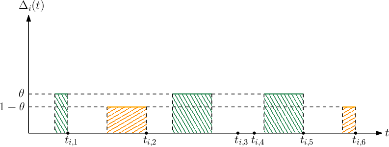
An estimation error happens when the actual infection status of the $i$th person, $x_{i}(t)$, is different than the estimate of the health care provider, $\hat{x}_{i}(t)$, at time $t$. This could happen in two ways: when $x_{i}(t)=1$ and $\hat{x}_{i}(t)=0$, i.e., when the $i$th person is sick, but it has not been detected by the health care provider, and when $x_{i}(t)=0$ and $\hat{x}_{i}(t)=1$, i.e., when the $i$th person has recovered, but the health care provider does not know that the $i$th person has recovered.

We denote the error caused by the former case, i.e., when $x_{i}(t)=1$ and $\hat{x}_{i}(t)=0$, by $\Delta_{i1}(t)$ (green areas in Fig. 2(b)),

and we denote the error caused by the latter case, i.e., when $x_{i}(t)=0$ and $\hat{x}_{i}(t)=1$, by $\Delta_{i2}(t)$ (orange areas in Fig. 2(b)),

Then, the total estimation error for the $i$th person $\Delta_{i}(t)$ is

where $\theta$ is the importance factor in $[0,1]$. A large $\theta$ gives more importance to the detection of infected people, and a small $\theta$ gives more importance to the detection of recovered people.

We define the long-term weighted average difference between $x_{i}(t)$ and $\hat{x}_{i}(t)$ as

Then, the overall average difference of all people $\Delta$ is

Our aim is to track the infection status of all people. Due to limited resources, there is a total test rate constraint $\sum_{i=1}^{n}s_{i}+\sum_{i=1}^{n}c_{i}\leq C$. Thus, our aim is to find the optimal test rates $s_{i}$ and $c_{i}$ to minimize $\Delta$ in (7) while satisfying this total test rate constraint. We formulate the following problem,

In the next section, we find the total average difference $\Delta$.

We first find analytical expressions for $\Delta_{i1}(t)$ in (3) and $\Delta_{i2}(t)$ in (4) when $s_{i}>0$ and $c_{i}>0$. We note that $\Delta_{i1}(t)$ can be equal to $1$ when $\hat{x}_{i}(t)=0$ and is always equal to $0$ when $\hat{x}_{i}(t)=1$. Assume that at time $0$, both $x_{i}(0)$ and $\hat{x}_{i}(0)$ are 0. After an exponentially distributed time with rate $\lambda_{i}$, which is denoted by $W_{i}$, the $i$th person is infected, and thus $x_{i}(t)$ becomes $1$. At that time, since $\hat{x}_{i}(t)=0$, $\Delta_{i1}(t)$ becomes $1$. $\Delta_{i1}(t)$ will be equal to 0 again either when the $i$th person recovers from the disease which happens after $R_{i}$ which is exponentially distributed with rate $\mu_{i}$ or when the health care provider performs a test on the $i$th person after $D_{i}$ which is exponentially distributed with rate $s_{i}$. We define $T_{m}(i)$ as the earliest time at which one of these two cases happens, i.e., $T_{m}(i)=\min\{R_{i},D_{i}\}$. We note that $T_{m}(i)$ is also exponentially distributed with rate $\mu_{i}+s_{i}$, and we have $\mathbb{P}(T_{m}(i)=R_{i})=\frac{\mu_{i}}{\mu_{i}+s_{i}}$ and $\mathbb{P}(T_{m}(i)=D_{i})=\frac{s_{i}}{\mu_{i}+s_{i}}$. If the $i$th person recovers from the disease before testing, we return to the initial case where both $x_{i}(t)$ and $\hat{x}_{i}(t)$ are equal to $0$ again. In this case, this cycle repeats itself, i.e., the $i$th person becomes sick again after $W_{i}$ and $\Delta_{i1}(t)$ remains as 1 until either the person recovers or the health care provider performs a test which takes another $T_{m}(i)$ duration. If the health care provider performs a test before the person recovers, then $\hat{x}_{i}(t)$ becomes $1$. We denote the time interval for which $\hat{x}_{i}(t)$ stays at 0 as $I_{i1}$ which is given by

where $K_{1}$ is geometric with rate $\mathbb{P}(T_{m}(i)=D_{i})=\frac{s_{i}}{\mu_{i}+s_{i}}$. Due to [103, Prob. 9.4.1], $\sum_{\ell=1}^{K_{1}}T_{m}(i,\ell)$ and $\sum_{\ell=1}^{K_{1}}W_{i}(\ell)$ are exponentially distributed with rates $s_{i}$ and $\frac{\lambda_{i}s_{i}}{\mu_{i}+s_{i}}$, respectively. As $\mathbb{E}[I_{i1}]=\mathbb{E}[\sum_{\ell=1}^{K_{1}}T_{m}(i,\ell)]+\mathbb{E}[\sum_{\ell=1}^{K_{1}}W_{i}(\ell)]$, we have

When $\hat{x}_{i}(t)=1$, the health care provider marks the $i$th person as infected. The $i$th person recovers from the virus after $R_{i}$. After the $i$th person recovers, either the health care provider performs a test after $Z_{i}$ which is exponentially distributed with rate $c_{i}$ or the $i$th person is reinfected with the virus which takes $W_{i}$ time. We define $T_{u}(i)$ as the earliest time at which one of these two cases happens, i.e., $T_{u}(i)=\min\{W_{i},Z_{i}\}$. Similarly, we note that $T_{u}(i)$ is exponentially distributed with rate $\lambda_{i}+c_{i}$, and we have $\mathbb{P}(T_{u}(i)=W_{i})=\frac{\lambda_{i}}{\lambda_{i}+c_{i}}$ and $\mathbb{P}(T_{u}(i)=Z_{i})=\frac{c_{i}}{\lambda_{i}+c_{i}}$. If the person is reinfected with the virus before a test is applied, this cycle repeats itself, i.e., the $i$th person recovers after another $R_{i}$, and then either a test is applied to the $i$th person, or the person is infected again which takes another $T_{u}(i)$. If the health care provider performs a test to the $i$th person before the person is reinfected, the health care provider marks the $i$th person as healthy again, i.e., $\hat{x}_{i}(t)$ becomes 0. We denote the time interval that $\hat{x}_{i}(t)$ is equal to 1 as $I_{i2}$ which is given by

where $K_{2}$ is geometric with rate $\mathbb{P}(T_{u}(i)=Z_{i})=\frac{c_{i}}{\lambda_{i}+c_{i}}$. Similarly, $\sum_{\ell=1}^{K_{2}}T_{u}(i,\ell)$ and $\sum_{\ell=1}^{K_{2}}R_{i}(\ell)$ are exponentially distributed with rates $c_{i}$ and $\frac{c_{i}\mu_{i}}{\lambda_{i}+c_{i}}$, respectively. As $\mathbb{E}[I_{i2}]=\mathbb{E}[\sum_{\ell=1}^{K_{2}}T_{u}(i,\ell)]+\mathbb{E}[\sum_{\ell=1}^{K_{2}}R_{i}(\ell)]$, we have

We denote the time interval between the $j$th and $(j+1)$th times that $\hat{x}_{i}(t)$ changes from 1 to 0 as the $j$th cycle $I_{i}(j)$ where $I_{i}(j)=I_{i1}(j)+I_{i2}(j)$. We note that $\Delta_{i1}(t)$ is always equal to 0 during $I_{i2}(j)$, i.e., $\hat{x}_{i}(t)=1$, and $\Delta_{i1}(t)$ is equal to 1 when $x_{i}(t)=1$ in $I_{i1}(j)$. We denote the total time duration when $\Delta_{i1}(t)$ is equal to 1 as $T_{e,1}(i,j)$ during the $j$th cycle where $T_{e,1}(i,j)=\sum_{\ell=1}^{K_{1}}T_{m}(i,\ell)$. Thus, we have $\mathbb{E}[T_{e,1}(i)]=\frac{1}{s_{i}}$. Then, using ergodicity, similar to [80], $\Delta_{i1}$ is equal to

Thus, we have

Next, we find $\Delta_{i2}$. We note that $\Delta_{i2}(t)$ is equal to 1 when $x_{i}(t)=0$ in $I_{i2}(j)$ and is always equal to 0 during $I_{i1}(j)$. Similarly, we denote the total time duration where $\Delta_{i2}(t)$ is equal to 1 in the $j$th cycle $I_{i}(j)$ as $T_{e,2}(i,j)$ which is equal to $T_{e,2}(i,j)=\sum_{\ell=1}^{K_{2}}T_{u}(i,\ell)$. Thus, we have $\mathbb{E}[T_{e,2}(i)]=\frac{1}{c_{i}}$. Then, similar to $\Delta_{i1}$ in (13), $\Delta_{i2}$ is equal to

By using (5), (14), and (15), we obtain $\Delta_{i}$ as

Then, by inserting (16) in (7), we obtain $\Delta$. In the next section, we solve the optimization problem in (II).

In this section, we solve the optimization problem in (II). Using $\Delta_{i}$ in (16) in (7), we rewrite (II) as

We define the Lagrangian function [104] for (IV) as

where $\beta\geq 0$, $\nu_{i}\geq 0$, and $\eta_{i}\geq 0$. The KKT conditions are

for all $i$. The complementary slackness conditions are

First, we find $s_{i}$. From (19), we have

When $\theta(c_{i}+\lambda_{i})\geq(1-\theta)\mu_{i}$, we solve (22) for $s_{i}$ as

where we used the fact that we either have $s_{i}>0$ and $\nu_{i}=0$, or $s_{i}=0$ and $\nu_{i}\geq 0$, due to (21). Here, $(\cdot)^{+}=\max(\cdot,0)$. On the other hand, when $\theta(c_{i}+\lambda_{i})<(1-\theta)\mu_{i}$, we have $\frac{\partial\Delta_{i}}{\partial s_{i}}>0$, and thus it is optimal to choose $s_{i}=0$ as our aim is to minimize $\Delta$ in (7). In this case, when $s_{i}=0$, we have $\Delta_{i}=\frac{\theta\lambda_{i}}{\mu_{i}+\lambda_{i}}$ which is independent of the value of $c_{i}$. As we obtain the same $\Delta_{i}$ for all values of $c_{i}$, and the total update rate is limited, i.e., $\sum_{i=1}^{n}s_{i}+c_{i}\leq C$, in this case, it is optimal to choose $c_{i}=0$ as well (i.e., when $s_{i}=0$).

Next, we find $c_{i}$. From (20), we have

When $(1-\theta)(\mu_{i}+s_{i})\geq\theta\lambda_{i}$, we solve (24) for $c_{i}$ as

where we used the fact that we either have $c_{i}>0$ and $\eta_{i}=0$, or $c_{i}=0$ and $\eta_{i}\geq 0$, due to (21). Similarly, when $(1-\theta)(s_{i}+\mu_{i})<\theta\lambda_{i}$, we have $\frac{\partial\Delta_{i}}{\partial c_{i}}>0$. Thus, in this case, it is optimal to choose $c_{i}=0$. When $c_{i}=0$, we have $\Delta_{i}=\frac{(1-\theta)\mu_{i}}{\mu_{i}+\lambda_{i}}$ which is independent of the value of $s_{i}$. Thus, it is optimal to choose $s_{i}=0$ when $c_{i}=0$.

From (23), if $\frac{1}{\mu_{i}c_{i}}\frac{\lambda_{i}}{\mu_{i}+\lambda_{i}}(\theta(c_{i}+\lambda_{i})-(1-\theta)\mu_{i})\leq\beta$, we must have $s_{i}=0$. Thus, for a given $c_{i}$, the optimal test rate allocation policy for $s_{i}$ is a threshold policy where $s_{i}$’s with small $\frac{1}{\mu_{i}c_{i}}\frac{\lambda_{i}}{\mu_{i}+\lambda_{i}}(\theta(c_{i}+\lambda_{i})-(1-\theta)\mu_{i})$ are equal to zero. Similarly, from (25), if $\frac{1}{\lambda_{i}s_{i}}\frac{\mu_{i}}{\mu_{i}+\lambda_{i}}\left((1-\theta)(s_{i}+\mu_{i})-\theta\lambda_{i}\right)\leq\beta$, we must have $c_{i}=0$. Thus, for a given $s_{i}$, the optimal policy to determine $c_{i}$ is a threshold policy where $c_{i}$’s with small $\frac{1}{\lambda_{i}s_{i}}\frac{\mu_{i}}{\mu_{i}+\lambda_{i}}((1-\theta)(s_{i}+\mu_{i})-\theta\lambda_{i})$ are equal to zero.

Next, we show that in the optimal policy, if $s_{i}>0$ and $c_{i}>0$ for some $i$, then the total test rate constraint must be satisfied with equality, i.e., $\sum_{i=1}^{n}s_{i}+c_{i}=C$.

Next, we propose an alternating minimization based algorithm for finding $s_{i}$ and $c_{i}$. For this purpose, for given initial $(s_{i},c_{i})$ pairs, we define $\phi_{i}$ as

Then, we define $u_{i}$ as

From (23) and (25), $s_{i}=u_{i}$ and $c_{i}=u_{n+i}$, for $i=1,\dots,n$.

Next, we find $s_{i}$ and $c_{i}$ by determining $\beta$ in (29). First, assume that, in the optimal policy, there is an $i$ such that $s_{i}>0$ and $c_{i}>0$. Thus, by Lemma 1, we must have $\sum_{i=1}^{n}s_{i}+c_{i}=C$. We initially take random $(s_{i},c_{i})$ pairs such that $\sum_{i=1}^{n}s_{i}+c_{i}=C$. Then, given the initial $(s_{i},c_{i})$ pairs, we immediately choose $u_{i}=0$ for $\phi_{i}<0$. For the remaining $u_{i}$ with $\phi_{i}\geq 0$, we apply a solution method similar to that in [80]. By assuming $\phi_{i}\geq\beta$, i.e., by disregarding $(\cdot)^{+}$ in (29), we solve $\sum_{i=1}^{2n}u_{i}=C$ for $\beta$. Then, we compare the smallest $\phi_{i}$ which is larger than zero in (28) with $\beta$. If we have $\phi_{i}\geq\beta$, then it implies that $u_{i}\geq 0$ for all remaining $i$. Thus, we have obtained $u_{i}$ values for given initial ($s_{i},c_{i}$) pairs. If the smallest $\phi_{i}$ which is larger than zero is smaller than $\beta$, then the corresponding $u_{i}$ is negative and we should choose $u_{i}=0$ for the smallest non-negative $\phi_{i}$. Then, we repeat this procedure until the smallest non-negative $\phi_{i}$ is larger than $\beta$. After determining all $u_{i}$, we obtain $s_{i}=u_{i}$ and $c_{i}=u_{n+i}$ for $i=1,\dots,n$. Then, with the updated values of $(s_{i},c_{i})$ pairs, we keep finding $u_{i}$’s until the KKT conditions in (19) and (20) are satisfied.

We note that for indices (persons) $i$ for which $(s_{i},c_{i})$ are zero, the health care provider does not perform any tests, and maps these people as either always infected, i.e., $\hat{x}_{i}(t)=1$ for all $t$, or always healthy, i.e., $\hat{x}_{i}(t)=0$. If $\hat{x}_{i}(t)=0$ for all $t$, $\Delta_{i}=\frac{\theta\lambda_{i}}{\mu_{i}+\lambda_{i}}$, and if $\hat{x}_{i}(t)=1$ for all $t$, $\Delta_{i}=\frac{(1-\theta)\mu_{i}}{\mu_{i}+\lambda_{i}}$. Thus, for such $i$, the health care provider should choose $\hat{x}_{i}(t)=0$ for all $t$, if $\frac{\theta\lambda_{i}}{\mu_{i}+\lambda_{i}}<\frac{(1-\theta)\mu_{i}}{\mu_{i}+\lambda_{i}}$, and should choose $\hat{x}_{i}(t)=1$ for all $t$, otherwise, without performing any tests.

Finally, we note that the problem in (IV) is not a convex optimization problem as the objective function is not jointly convex in $s_{i}$ and $c_{i}$. Therefore, the solutions obtained via the proposed method may not be globally optimal. For that reason, we choose different initial starting points and apply the proposed alternating minimization based algorithm and choose the solution that achieves the smallest $\Delta$ in (7).

In the next section, we first provide an alternative way to find the average difference $\Delta$ in (6) and then characterize the average difference for the erroneous test measurements.

We note that the infection status of the $i$th person and its estimate at the health care provider form a continuous time Markov chain [105, Section 7.5] with the states $(x_{i}(t),\hat{x}_{i}(t))\in\{(0,0),\\ (0,1),(1,0),(1,1)\}$. In this section, by finding the steady-state distribution for $(x_{i}(t),\hat{x}_{i}(t))$, we provide an alternative method to find $\Delta$ in (6). Then, we consider the case with erroneous test measurements. For this case, we characterize the long-term average difference for the $i$th person denoted by $\Delta_{i}^{e}$.

References

- [1] S. K. Kaul, R. D. Yates, and M. Gruteser, “Real-time status: How often should one update?,” in IEEE Infocom, March 2012.
- [2] I. Kadota, A. Sinha, E. Uysal-Biyikoglu, R. Singh, and E. Modiano, “Scheduling policies for minimizing age of information in broadcast wireless networks,” IEEE/ACM Transactions on Networking, vol. 26, no. 6, pp. 2637–2650, December 2018.
- [3] C. Kam, S. Kompella, G. D. Nguyen, J. E. Wieselthier, and A. Ephremides, “Age of information with a packet deadline,” in IEEE ISIT, July 2016.
- [4] Y. Sun, E. Uysal-Biyikoglu, R. D. Yates, C. E. Koksal, and N. B. Shroff, “Update or wait: How to keep your data fresh,” IEEE Transactions on Information Theory, vol. 63, no. 11, pp. 7492–7508, November 2017.
- [5] E. Najm and E. Telatar, “Status updates in a multi-stream M/G/1/1 preemptive queue,” in IEEE Infocom, April 2018.
- [6] A. Soysal and S. Ulukus, “Age of information in G/G/1/1 systems: Age expressions, bounds, special cases, and optimization,” IEEE Transactions on Information Theory, vol. 67, pp. 7477–7489, July 2021.
- [7] B. Buyukates and S. Ulukus, “Age of information with Gilbert-Elliot servers and samplers,” in CISS, March 2020.
- [8] R. D. Yates, “The age of information in networks: Moments, distributions, and sampling,” IEEE Transactions on Information Theory, vol. 66, pp. 5712–5728, May 2020.
- [9] R. Talak, S. Karaman, and E. Modiano, “Minimizing age-of-information in multi-hop wireless networks,” in Allerton Conference, October 2017.
- [10] V. Tripathi and S. Moharir, “Age of information in multi-source systems,” in IEEE Globecom, December 2017.
- [11] A. M. Bedewy, Y. Sun, and N. B. Shroff, “The age of information in multihop networks,” IEEE/ACM Transactions on Networking, vol. 27, pp. 1248–1257, June 2019.
- [12] J. Zhong, R. D. Yates, and E. Soljanin, “Multicast with prioritized delivery: How fresh is your data?,” in IEEE SPAWC, June 2018.
- [13] B. Buyukates, A. Soysal, and S. Ulukus, “Age of information in two-hop multicast networks,” in Asilomar Conference, October 2018.
- [14] B. Buyukates, A. Soysal, and S. Ulukus, “Age of information in multihop multicast networks,” Journal of Communications and Networks, vol. 21, no. 3, pp. 256–267, July 2019.
- [15] B. Buyukates, A. Soysal, and S. Ulukus, “Age of information in multicast networks with multiple update streams,” in Asilomar Conference, November 2019.
- [16] K. S. A. Krishnan and V. Sharma, “Minimizing age of information in a multihop wireless network,” in IEEE ICC, June 2020.
- [17] S. Farazi, A. G. Klein, and D. R. Brown III, “Fundamental bounds on the age of information in multi-hop global status update networks,” Journal of Communications and Networks, vol. 21, no. 3, pp. 268–279, July 2019.
- [18] S. Ioannidis, A. Chaintreau, and L. Massoulie, “Optimal and scalable distribution of content updates over a mobile social network,” in IEEE Infocom, April 2009.
- [19] M. Wang, W. Chen, and A. Ephremides, “Reconstruction of counting process in real-time: The freshness of information through queues,” in IEEE ICC, July 2019.
- [20] Y. Sun, Y. Polyanskiy, and E. Uysal-Biyikoglu, “Remote estimation of the Wiener process over a channel with random delay,” in IEEE ISIT, June 2017.
- [21] Y. Sun and B. Cyr, “Information aging through queues: A mutual information perspective,” in IEEE SPAWC, June 2018.
- [22] J. Chakravorty and A. Mahajan, “Remote estimation over a packet-drop channel with Markovian state,” IEEE Transactions on Automatic Control, vol. 65, pp. 2016–2031, July 2020.
- [23] C. Kam, S. Kompella, and A. Ephremides, “Age of incorrect information for remote estimation of a binary Markov source,” in IEEE Infocom, July 2020.
- [24] A. Arafa, K. Banawan, K. G. Seddik, and H. V. Poor, “Sample, quantize and encode: Timely estimation over noisy channels,” IEEE Transactions on Communications, 2021. To appear. Available on arXiv:2007.10200.
- [25] M. Bastopcu and S. Ulukus, “Who should Google Scholar update more often?,” in IEEE Infocom, July 2020.
- [26] B. T. Bacinoglu, Y. Sun, E. Uysal-Biyikoglu, and V. Mutlu, “Achieving the age-energy trade-off with a finite-battery energy harvesting source,” in IEEE ISIT, June 2018.
- [27] A. Baknina, O. Ozel, J. Yang, S. Ulukus, and A. Yener, “Sending information through status updates,” in IEEE ISIT, June 2018.
- [28] A. Baknina and S. Ulukus, “Coded status updates in an energy harvesting erasure channel,” in CISS, March 2018.
- [29] X. Wu, J. Yang, and J. Wu, “Optimal status update for age of information minimization with an energy harvesting source,” IEEE Transactions on Green Communications and Networking, vol. 2, no. 1, pp. 193–204, March 2018.
- [30] S. Feng and J. Yang, “Optimal status updating for an energy harvesting sensor with a noisy channel,” in IEEE Infocom, April 2018.
- [31] S. Feng and J. Yang, “Minimizing age of information for an energy harvesting source with updating failures,” in IEEE ISIT, June 2018.
- [32] A. Arafa, J. Yang, S. Ulukus, and H. V. Poor, “Age-minimal online policies for energy harvesting sensors with incremental battery recharges,” in UCSD ITA, February 2018.
- [33] A. Arafa, J. Yang, and S. Ulukus, “Age-minimal online policies for energy harvesting sensors with random battery recharges,” in IEEE ICC, May 2018.
- [34] A. Arafa, J. Yang, S. Ulukus, and H. V. Poor, “Age-minimal transmission for energy harvesting sensors with finite batteries: online policies,” IEEE Transactions on Information Theory, vol. 66, pp. 534–556, January 2020.
- [35] A. Arafa, J. Yang, S. Ulukus, and H. V. Poor, “Online timely status updates with erasures for energy harvesting sensors,” in Allerton Conference, October 2018.
- [36] A. Arafa, J. Yang, S. Ulukus, and H. V. Poor, “Using erasure feedback for online timely updating with an energy harvesting sensor,” in IEEE ISIT, July 2019.
- [37] A. Arafa, J. Yang, S. Ulukus, and H. V. Poor, “Timely status updating over erasure channels using an energy harvesting sensor: Single and multiple sources,” IEEE Transactions on Green Communications and Networking, vol. 6, pp. 6–19, March 2022.
- [38] S. Farazi, A. G. Klein, and D. R. Brown III, “Average age of information for status update systems with an energy harvesting server,” in IEEE Infocom, April 2018.
- [39] S. Leng and A. Yener, “Age of information minimization for an energy harvesting cognitive radio,” IEEE Transactions on Cognitive Communications and Networking, vol. 5, no. 2, pp. 427–439, June 2019.
- [40] Z. Chen, N. Pappas, E. Bjornson, and E. G. Larsson, “Age of information in a multiple access channel with heterogeneous traffic and an energy harvesting node,” in IEEE Infocom, April 2019.
- [41] R. V. Bhat, R. Vaze, and M. Motani, “Throughput maximization with an average age of information constraint in fading channels,” IEEE Transactions on Wireless Communications, vol. 20, pp. 481–494, January 2021.
- [42] J. Ostman, R. Devassy, G. Durisi, and E. Uysal, “Peak-age violation guarantees for the transmission of short packets over fading channels,” in IEEE Infocom, April 2019.
- [43] M. Bastopcu and S. Ulukus, “Age of information with soft updates,” in Allerton Conference, October 2018.
- [44] M. Bastopcu and S. Ulukus, “Minimizing age of information with soft updates,” Journal of Communications and Networks, vol. 21, no. 3, pp. 233–243, July 2019.
- [45] B. Buyukates, A. Soysal, and S. Ulukus, “Age of information scaling in large networks,” in IEEE ICC, May 2019.
- [46] B. Buyukates, A. Soysal, and S. Ulukus, “Age of information scaling in large networks with hierarchical cooperation,” in IEEE Globecom, December 2019.
- [47] B. Buyukates, A. Soysal, and S. Ulukus, “Scaling laws for age of information in wireless networks,” IEEE Transactions on Wireless Communications, vol. 20, pp. 2413–2427, April 2021.
- [48] J. Zhong, R. D. Yates, and E. Soljanin, “Minimizing content staleness in dynamo-style replicated storage systems,” in IEEE Infocom, April 2018.
- [49] N. Rajaraman, R. Vaze, and G. Reddy, “Not just age but age and quality of information,” IEEE Journal on Selected Areas in Communications, vol. 39, pp. 1325–1338, May 2021.
- [50] Z. Liu and B. Ji, “Towards the tradeoff between service performance and information freshness,” in IEEE ICC, May 2019.
- [51] A. Maatouk, M. Assaad, and A. Ephremides, “The age of incorrect information: an enabler of semantics-empowered communication,” December 2020. Available on arXiv:2012.13214.
- [52] E. Uysal, O. Kaya, A. Ephremides, J. Gross, M. Codreanu, P. Popovski, M. Assaad, G. Liva, A. Munari, T. Soleymani, B. Soret, and K. H. Johansson, “Semantic communications in networked systems,” March 2021. Available on arXiv:2103.05391.
- [53] O. Ayan, M. Vilgelm, M. Kluge, S. Hirche, and W. Kellerer, “Age-of-information vs. value-of-information scheduling for cellular networked control systems,” in ACM/IEEE ICCPS, April 2019.
- [54] M. Bastopcu and S. Ulukus, “Timely group updating,” in CISS, March 2021.
- [55] S. Banerjee, R. Bhattacharjee, and A. Sinha, “Fundamental limits of age-of-information in stationary and non-stationary environments,” in IEEE ISIT, June 2020.
- [56] J. Zhong and R. D. Yates, “Timeliness in lossless block coding,” in IEEE DCC, March 2016.
- [57] J. Zhong, R. D. Yates, and E. Soljanin, “Timely lossless source coding for randomly arriving symbols,” in IEEE ITW, November 2018.
- [58] P. Mayekar, P. Parag, and H. Tyagi, “Optimal lossless source codes for timely updates,” in IEEE ISIT, June 2018.
- [59] P. Mayekar, P. Parag, and H. Tyagi, “Optimal source codes for timely updates,” IEEE Transactions on Information Theory, vol. 66, pp. 3714–3731, March 2020.
- [60] M. Bastopcu, B. Buyukates, and S. Ulukus, “Optimal selective encoding for timely updates,” in CISS, March 2020.
- [61] B. Buyukates, M. Bastopcu, and S. Ulukus, “Optimal selective encoding for timely updates with empty symbol,” in IEEE ISIT, June 2020.
- [62] M. Bastopcu, B. Buyukates, and S. Ulukus, “Selective encoding policies for maximizing information freshness,” IEEE Transactions on Communications, vol. 69, pp. 5714–5726, September 2021.
- [63] D. Ramirez, E. Erkip, and H. V. Poor, “Age of information with finite horizon and partial updates,” in IEEE ICASSP, May 2020.
- [64] A. Arafa, K. Banawan, K. G. Seddik, and H. V. Poor, “On timely channel coding with hybrid ARQ,” in IEEE Globecom, December 2019.
- [65] A. Arafa and R. D. Wesel, “Timely transmissions using optimized variable length coding,” in IEEE Infocom, May 2021.
- [66] M. Bastopcu and S. Ulukus, “Partial updates: Losing information for freshness,” in IEEE ISIT, June 2020.
- [67] M. A. Abd-Elmagid and H. S. Dhillon, “Average peak age-of-information minimization in UAV-assisted IoT networks,” IEEE Transactions on Vehicular Technology, vol. 68, no. 2, pp. 2003–2008, February 2019.
- [68] J. Liu, X. Wang, and H. Dai, “Age-optimal trajectory planning for UAV-assisted data collection,” in IEEE Infocom, April 2018.
- [69] M. A. Abd-Elmagid, N. Pappas, and H. S. Dhillon, “On the role of age of information in the internet of things,” IEEE Communications Magazine, vol. 57, no. 12, pp. 72–77, December 2019.
- [70] A. Alabbasi and V. Aggarwal, “Joint information freshness and completion time optimization for vehicular networks,” IEEE Transactions on Services Computing, pp. 1–14, March 2020.
- [71] W. Gao, G. Cao, M. Srivatsa, and A. Iyengar, “Distributed maintenance of cache freshness in opportunistic mobile networks,” in IEEE ICDCS, June 2012.
- [72] R. D. Yates, P. Ciblat, A. Yener, and M. Wigger, “Age-optimal constrained cache updating,” in IEEE ISIT, June 2017.
- [73] C. Kam, S. Kompella, G. D. Nguyen, J. E. Wieselthier, and A. Ephremides, “Information freshness and popularity in mobile caching,” in IEEE ISIT, June 2017.
- [74] S. Zhang, J. Li, H. Luo, J. Gao, L. Zhao, and X. S. Shen, “Towards fresh and low-latency content delivery in vehicular networks: An edge caching aspect,” in IEEE WCSP, October 2018.
- [75] H. Tang, P. Ciblat, J. Wang, M. Wigger, and R. Yates, “Age of information aware cache updating with file- and age-dependent update durations,” in IEEE WiOpt, June 2020.
- [76] J. Zhong, R. D. Yates, and E. Soljanin, “Two freshness metrics for local cache refresh,” in IEEE ISIT, June 2018.
- [77] L. Yang, Y. Zhong, F. Zheng, and S. Jin, “Edge caching with real-time guarantees,” December 2019. Available on arXiv:1912.11847.
- [78] M. Bastopcu and S. Ulukus, “Maximizing information freshness in caching systems with limited cache storage capacity,” in Asilomar Conference, November 2020.
- [79] M. Bastopcu and S. Ulukus, “Cache freshness in information updating systems,” in CISS, March 2021.
- [80] M. Bastopcu and S. Ulukus, “Information freshness in cache updating systems,” IEEE Transactions on Wireless Communications, vol. 20, pp. 1861–1874, March 2021.
- [81] P. Kaswan, M. Bastopcu, and S. Ulukus, “Freshness based cache updating in parallel relay networks,” in IEEE ISIT, July 2021.
- [82] Y. Gu, Q. Wang, H. Chen, Y. Li, and B. Vucetic, “Optimizing information freshness in two-hop status update systems under a resource constraint,” IEEE Journal on Selected Areas in Communications, vol. 39, pp. 1380–1392, May 2021.
- [83] Q. Kuang, J. Gong, X. Chen, and X. Ma, “Age-of-information for computation-intensive messages in mobile edge computing,” January 2019. Available on arXiv: 1901.01854.
- [84] J. Gong, Q. Kuang, X. Chen, and X. Ma, “Reducing age-of-information for computation-intensive messages via packet replacement,” in IEEE WCSP, October 2019.
- [85] P. Zou, O. Ozel, and S. Subramaniam, “Trading off computation with transmission in status update systems,” in IEEE PIMRC, September 2019.
- [86] M. Bastopcu and S. Ulukus, “Age of information for updates with distortion,” in IEEE ITW, August 2019.
- [87] M. Bastopcu and S. Ulukus, “Age of information for updates with distortion: Constant and age-dependent distortion constraints,” IEEE/ACM Transactions on Networking, vol. 29, pp. 2425–2438, December 2021.
- [88] B. Buyukates and S. Ulukus, “Timely updates in distributed computation systems with stragglers,” in Asilomar Conference, November 2020.
- [89] B. Buyukates and S. Ulukus, “Timely distributed computation with stragglers,” IEEE Transactions on Communications, vol. 68, pp. 5273–5282, September 2020.
- [90] P. Zou, O. Ozel, and S. Subramaniam, “Optimizing information freshness through computation–transmission tradeoff and queue management in edge computing,” IEEE/ACM Transactions on Networking, vol. 29, pp. 949–963, April 2021.
- [91] B. Buyukates and S. Ulukus, “Timely communication in federated learning,” in IEEE Infocom, May 2021.
- [92] E. Ozfatura, B. Buyukates, D. Gunduz, and S. Ulukus, “Age-based coded computation for bias reduction in distributed learning,” in IEEE Globecom, December 2020.
- [93] E. T. Ceran, D. Gündüz, and A. György, “A reinforcement learning approach to age of information in multi-user networks with HARQ,” IEEE Journal on Selected Areas in Communications, vol. 39, pp. 1412–1426, May 2021.
- [94] R. D. Yates, “The age of gossip in networks,” in IEEE ISIT, July 2021.
- [95] B. Buyukates, M. Bastopcu, and S. Ulukus, “Age of gossip in networks with community structure,” in IEEE SPAWC, September 2021.
- [96] M. Bastopcu, B. Buyukates, and S. Ulukus, “Gossiping with binary freshness metric,” in IEEE Globecom, December 2021.
- [97] P. Kaswan and S. Ulukus, “Timely gossiping with file slicing and network coding,” February 2022. Available on arXiv:2202.00649.
- [98] A. Kosta, N. Pappas, and V. Angelakis, “Age of information: A new concept, metric, and tool,” Foundations and Trends in Networking, vol. 12, pp. 162–259, November 2017.
- [99] Y. Sun, I. Kadota, R. Talak, and E. Modiano, “Age of information: A new metric for information freshness,” Synthesis Lectures on Communication Networks, vol. 12, pp. 1–224, December 2019.
- [100] R. D. Yates, Y. Sun, D. R. Brown III, S. K. Kaul, E. Modiano, and S. Ulukus, “Age of information: An introduction and survey,” IEEE Journal on Selected Areas in Communications, vol. 39, pp. 1183–1210, May 2021.
- [101] J. Yun, C. Joo, and A. Eryilmaz, “Optimal real-time monitoring of an information source under communication costs,” in IEEE CDC, December 2018.
- [102] A. Maatouk, S. Kriouile, M. Assaad, and A. Ephremides, “The age of incorrect information: A new performance metric for status updates,” IEEE/ACM Transactions on Networking, vol. 28, pp. 2215–2228, July 2020.
- [103] R. D. Yates and D. J. Goodman, Probability and Stochastic Processes. Wiley, 2014.
- [104] S. P. Boyd and L. Vandenberghe, Convex Optimization. Cambridge University Press, 2004.
- [105] D. P. Bertsekas and J. N. Tsitsiklis, Introduction to Probability. Athena Scientific, 2008.
- [106] Y. C. Chen, P. E. Lu, C. S. Chang, and T. H. Liu, “A time-dependent SIR model for covid-19 with undetectable infected persons,” IEEE Transactions on Network Science and Engineering, vol. 7, no. 4, pp. 3279–3294, 2020.
- [107] S. Y. Olmez, J. Mori, E. Miehling, T. Başar, R. L. Smith, M. West, and P. G. Mehta, “A data-informed approach for analysis, validation, and identification of covid-19 models,” in IEEE ACC, May 2021.