Real-space Bell inequalities in de Sitter

Here we summarise the proposal made in Ref. [40] to cast two-point measurements of a quantum field in terms of a quantum bipartite system. Only the main arguments and results are given, while further details can be found in Ref. [40]. Let $\phi(\vec{x})$ be a real scalar quantum field (since all measurements are performed at the same time, the time argument is omitted for notation convenience) and $\pi(\vec{x})$ its conjugated momentum. We define the field coarse-grained at a location $\vec{x}$ over a radius $R$ as

with a similar expression for $\pi_{R}(\vec{x})$. In this formula, $a$ is the scale factor of the universe, such that space is labelled by comoving coordinates,¹¹ 1 This is to make the formalism directly applicable to cosmology in Sec. 4. Otherwise, in flat space-time, one may simply set $a=1$ and use physical coordinates, as in Sec. 3. and $W$ is a window function that asymptotes a constant at small arguments and decays at large arguments. It is normalised such that $\int_{0}^{\infty}z^{2}W(z)\differential z=1/(4\pi)$, i.e. such that a uniform field is left invariant by the coarse-graining procedure. Moreover, in order for the field and its momentum to commute when coarse-grained around distant spatial locations, the support of $W$ must be taken as compact. In practice, we assume that $W(z)=0$ for $z\geq 1+\delta$, i.e. $\delta$ is a parameter that controls the size of the support of $W$ [see Eq. (2.18) below]. Let us then consider two spatial points $\vec{x}_{1}$ and $\vec{x}_{2}$ distant by $d\equiv a|\vec{x}_{1}-\vec{x}_{2}|>2R(1+\delta)$ (the situation is summarised in Fig. 1). One has $[\phi_{R}(\vec{x}_{1}),\phi_{R}(\vec{x}_{2})]=[\pi_{R}(\vec{x}_{1}),\pi_{R}(\vec{x}_{2})]=0$, while thanks to the compactness of $W$, the canonical commutation relation $[\phi(\vec{x}),\pi(\vec{y})]=i\delta(\vec{x}-\vec{y})$ ensures that

which defines the parameter $G$, and where the prefactor is arranged such that $G=1$ for a constant window function with $\delta=0$. As a consequence, canonical commutation relations for the coarse-grained fields are recovered only after rescaling the fields according to

The coarse-grained rescaled fields thus describe a bipartite system with canonical commutation relations, which was the goal of this subsection.

Our next task is to introduce pseudo-spin operators for the continuous variables describing those coarse-grained rescaled fields. The construction of spin operators out of continuous variables can be addressed in several ways, see Ref. [20] for various proposals. Here, for expliciteness, we consider the so-called Gour-Khanna-Mann-Revzen (GKMR) pseudo-spin operators [32, 28], although another set of spin operators will be discussed in Sec. 5.

GKMR operators are built from the eigenstates $\ket{\tilde{\phi}_{R}(\vec{x})}$ of the coarse-grained field configuration. Let us first introduce the auxiliary states

in terms of which the GKMR operators are defined as

One can check that those operators are indeed pseudo-spin operators, i.e. they are such that $\hat{\mathcal{S}}_{x}^{2}=\hat{\mathcal{S}}_{y}^{2}=\hat{\mathcal{S}}_{z}^{2}=1$ and they satisfy the SU(2) commutation relations $[\hat{\mathcal{S}}_{x},\hat{\mathcal{S}}_{y}]=2i\hat{\mathcal{S}}_{z}$, $[\hat{\mathcal{S}}_{y},\hat{\mathcal{S}}_{z}]=2i\hat{\mathcal{S}}_{x}$ and $[\hat{\mathcal{S}}_{z},\hat{\mathcal{S}}_{x}]=2i\hat{\mathcal{S}}_{y}$. Note also that since $\hat{\mathcal{S}}_{z}$ is diagonal in the field eigenvector basis, it involves the field operator only. On the contrary, $\hat{\mathcal{S}}_{x}$ and $\hat{\mathcal{S}}_{y}$ are not diagonal, hence they also rely on the momentum operator. As mentioned in Sec. 1, in a cosmological context, it implies that their measurement requires access to the decaying mode, which is technically challenging.

In order to perform explicit calculations, let us assume that the quantum field is placed in a Gaussian state. This case is particularly relevant for cosmology, since at linear order in cosmological perturbation theory, cosmological perturbations are indeed placed in such a state. Gaussian states are easy to represent in phase space, since their Wigner function is simply given by a Gaussian function

where we have arranged the bipartite phase-space variables into the vector ${\bm{q}}=(\tilde{\phi}_{R}(\vec{x}_{1}),\tilde{\pi}_{R}(\vec{x}_{1}),\allowbreak\tilde{\phi}_{R}(\vec{x}_{2}),\tilde{\pi}_{R}(\vec{x}_{2}))^{\mathrm{T}}$. Let us recall that the Wigner function is constructed from the density matrix of the state via a Wigner-Weyl transform [41, 42, 43]

It is a phase-space function that gives a full representation of the quantum state (given that the density matrix can be recovered from the Wigner function by an inverse Wigner-Weyl transform). This representation is particularly convenient for Gaussian states given its simple form (2.7), and we choose to work with it since it makes the following calculations technically much simpler.

In Eq. (2.7), ${\bm{\gamma}}$ is the covariance matrix of the system, i.e. it is such that [36]²² 2 Note that there is a factor $2$ difference in the definition of the covariance matrix with respect to Ref. [36].

where $\{\hat{A},\hat{B}\}\equiv(\hat{A}\hat{B}+\hat{B}\hat{A})/2$ denotes the anticommutator. The second expression above casts the result in terms of the Fourier transform of the window function $\widetilde{W}(z)\equiv 4z^{-3}\allowbreak\int_{0}^{\infty}W(u/z)u\sin u\,\differential u$, and in terms of the reduced power spectra of the field and its momentum, defined as $\langle\{\hat{\phi}_{\vec{k}}^{\dagger},\hat{\phi}_{\vec{k}^{\prime}}\}\rangle=2\pi^{2}k^{-3}\mathcal{P}_{\phi\phi}(k)\delta(\vec{k}-\vec{k}^{\prime})$ with similar expressions for $\mathcal{P}_{\phi\pi}$ and $\mathcal{P}_{\pi\pi}$. Here, the Fourier transform is defined as $\hat{\phi}(\vec{x})=(2\pi)^{-3/2}\int\differential\vec{k}e^{-i\vec{k}\cdot\vec{x}}\hat{\phi}(\vec{k})$ with a similar expression for $\hat{\pi}(x)$, and the above definition of the power spectrum assumes that the field is placed in a quantum state that is invariant under spatial translations and rotations, which is the case in cosmology.

Since the covariance matrix is symmetric, only the upper triangular part has been written explicitly. The invariance of the setup under exchanging subsystems 1 and 2 also leads to an additional symmetry of the covariance matrix, such that there are only $6$ independent entries, namely $\gamma_{11}$, $\gamma_{12}$, $\gamma_{22}$, $\gamma_{13}$, $\gamma_{14}$ and $\gamma_{24}$ (if the two coarse-graining radii are different at $\vec{x}_{1}$ and $\vec{x}_{2}$ then that symmetry is lost, but the present formalism can still be used, see Ref. [36]).

It is important to stress that even if the quantum state of the field is pure, the state of the bipartite system we consider is, in general, mixed. This can be seen by computing the purity parameter

which equals one for a pure state but is smaller than one otherwise, and where the second expression is valid for Gaussian states. By considering the configuration of the field in a subset of real space only (namely within a distance $R$ of either $\vec{x}_{1}$ or $\vec{x}_{2}$), our bipartite system is implicitly constructed by tracing over its configuration at every other location. By doing so, since the field is correlated in real space, one effectively obtains a mixed state, which explains why $\mathfrak{p}<1$. This “effective decoherence” mechanism [36, 40] has the potential to blur the presence of a genuine quantum signal. In Refs. [36, 40], its effect of quantum discord was investigated, while the goal of the present work is to study how it affects Bell-inequality violations.

Let us also note that the tracing-out procedure in the Hilbert space is equivalent to phase-space marginalisation (see Appendix D of Ref. [44]). As a consequence, the quantum state of the sub-system 1, which describes the field configuration around the location $\vec{x}_{1}$, can be alternatively obtained by (i) tracing the density matrix of the full bipartite system over the sub-system 2 or (ii) integrating the Wigner function (2.7) over $q_{3}$ and $q_{4}$. By following this second route, one still obtains a Gaussian Wigner function, the covariance matrix of which is simply given by the upper-left two-by-two sub-block of Eq. (2.9). This makes the phase-space representation of Gaussian states particularly convenient.

The Wigner-Weyl transform (2.8) can be written for any operator $\hat{O}$, which it hereby translates into a phase-space function $W_{\hat{O}}$. In the Wigner representation, its quantum expectation value is given by

The evaluation of the spin correlators $E(a,b)$ thus requires to first compute the Wigner-Weyl transform of the GKMR operators, and then to integrate it against the Wigner function (2.7). In each subspace, one finds [20]

where $\mathcal{P}$ denotes the principal part. Since $\hat{\mathcal{S}}_{i}(\vec{x}_{1})$ and $\hat{\mathcal{S}}_{j}(\vec{x}_{2})$ act on two separate sectors of the full Hilbert space, where $i$, $j=x$, $y$ or $z$, the Wigner-Weyl transform of their product is simply given by the product of their Wigner-Weyl transforms, i.e.

From the above expressions, one can thus readily compute the spin correlators in the state (2.7).

In general, one is free to set the directions of the spin measurements in an arbitrary way. It is however common practice to consider the case where $\hat{\mathcal{S}}_{a}=\hat{\mathcal{S}}_{z}$, $\hat{\mathcal{S}}_{a^{\prime}}=\hat{\mathcal{S}}_{x}$, and $\hat{\mathcal{S}}_{b}$ and $\hat{\mathcal{S}}_{b^{\prime}}$ are set in the $(xz)$ plane, i.e. $\hat{\mathcal{S}}_{b}=\sin\theta\hat{\mathcal{S}}_{x}+\cos\theta\hat{\mathcal{S}}_{z}$ and $\hat{\mathcal{S}}_{b^{\prime}}=\sin\theta^{\prime}\hat{\mathcal{S}}_{x}+\cos\theta^{\prime}\hat{\mathcal{S}}_{z}$. Since $\braket{\hat{\mathcal{S}}_{x}(\vec{x}_{1})\hat{\mathcal{S}}_{z}(\vec{x}_{2})}=0$ (see Appendix A), upon optimising the polar angles $\theta$ and $\theta^{\prime}$ such as to get a maximal value for $B$, one obtains

We are thus left with two spin correlators to compute. The details of this computation, which essentially boils down to performing Gaussian integrals, are deferred to Appendix A. One finds

where one recovers the purity parameter introduced in Eq. (2.10). This already indicates that the “effective decoherence” mechanism mentioned above leads to a suppression of the expectation value of the Bell operator, since $B=2\sqrt{\mathfrak{p}^{2}+\braket{\hat{\mathcal{S}}_{x}(\vec{x}_{1})\hat{\mathcal{S}}_{x}(\vec{x}_{2})}^{2}}$. One also has

where $a_{11}$, $a_{12}$ and $a_{22}$ are the entries of the symmetric two-by-two matrix

In this expression, the two overscripts indicate a restriction of the ${\bm{\gamma}}^{-1}$ matrix to the lines labelled by the first index, and to the columns labelled by the second index (see Appendix A for further details).

Before applying this formalism to concrete examples in Secs. 3 and 4, a last word is in order regarding the window function. As mentioned above, it needs to be compact for the phase-space operators at two different locations to commute, and the simplest choice is therefore to consider a Heaviside function. However, as pointed out in Refs. [36, 40], such a sharp window function sometimes creates divergences in some of the intermediate quantities being computed, and it is more convenient to consider a continuous window function that is made of a constant piece and of a linear piece:

where ${\mathcal{F}}(\delta)=(\delta+2)(\delta^{2}+2\delta+2)/4$ is such that the normalisation condition mentioned above is satisfied. With that expression, the Fourier transform of the window function is given by $\widetilde{W}(z)=3\{z\sin(z)-(1+\delta)z\sin\left[(1+\delta)z\right]+2\cos(z)-2\cos\left[(1+\delta)z\right]\}/[\delta\mathcal{F}(\delta)z^{4}]$, and one has $G(\delta)=8(\delta^{3}+5\delta^{2}+10\delta+10)/[5(\delta+2)^{2}(\delta^{2}+2\delta+2)^{2}]$.

After expanding the field into independent Fourier modes, the mode functions in the vacuum state are given by $\phi_{\vec{k}}=e^{-ikt}/\sqrt{2k}$ and $\pi_{\vec{k}}=\dot{\phi}_{\vec{k}}=-i\sqrt{k/2}e^{-ikt}$, which give rise to the reduced power spectra $\mathcal{P}_{\phi\phi}=k^{2}/(4\pi^{2})$, $\mathcal{P}_{\pi\pi}=k^{4}/(4\pi^{2})$ and $\mathcal{P}_{\phi\pi}=0$. Plugging those expressions into Eq. (2.9), the entries of the covariance matrix can be computed and are given by

where we have introduced the integrals

which depend on the parameter

This parameter measures the distance between the two patches in units of the patch radius, and as explained in Sec. 2.1, it needs to be larger than $2(1+\delta)$ for the two patches not to overlap. By plugging the expression for $\widetilde{W}$ given below Eq. (2.18) into Eq. (3.2), those integrals can be performed analytically, and the corresponding expressions can be found in Ref. [36]. We do not reproduce them here since they are not particularly insightful at this stage.

Let us now evaluate the GKMR spin correlators following the method outlined in Sec. 2.4. Since the field-momentum correlators vanish, namely $\gamma_{12}=\gamma_{14}=0$, one can show that it is also true for the inverse covariance matrix, i.e. $({\bm{\gamma}}^{-1})^{\phi\pi}={\bm{0}}$. As a consequence, Eq. (2.17) leads to

so Eqs. (2.16) and (2.15) give rise to

where the result is also given in terms of the integrals introduced in Eq. (3.2).

By plugging those expressions into Eq. (2.14), one obtains an explicit formula for the expectation value of the Bell operator in terms of the two parameter $\alpha$ and $\beta$. The result is displayed in the left panel of Fig. 2 for $\delta=0.01$ and as a function of $\alpha$. One can see that $B(\vec{x}_{1},\vec{x}_{2})$ decreases with $\alpha$ and reaches an asymptotic value at large distances between the two patches. This can be understood by expanding the above formulas in the limit where $\delta$ is small but $\alpha$ is large, which gives rise to

Together with Eq. (2.14), this leads to

which is displayed as the orange dashed line in Fig. 2. One can check that, when $\alpha\gg 1$, it provides a good fit to the full result indeed. At large $\alpha$, $B$ reaches a constant that is given by the first term of Eq. (3.7) and which is controlled by the purity of the state. It is displayed with the green dotted line. Note that the case $\delta=0$ is singular, and leads to $B\simeq 16/(9\pi\alpha^{2})$ at large $\alpha$ (so the asymptotic value vanishes).

Since $B$ is maximal when $\alpha$ is minimal, in the right panel of Fig. 2 we set $\alpha$ to its minimal value and let $\delta$ vary, so as to optimise the expectation value of the Bell operator. One can see that $B$ increases with $\delta$,³³ 3 When $\delta\to 0$, $\alpha_{\mathrm{min}}\to 2$ and one has $\mathcal{L}_{1}=3(13-16\ln 2)/20$, $\mathcal{L}_{3}=3(\ln 2-1)/2$, $\mathcal{K}_{1}=9/4$ and $\mathcal{K}_{3}$ diverges logarithmically with $\delta$. This leads to $B\simeq 0.16$, which corresponds to the lower asymptotic value in the right panel of Fig. 2 that would be reached if the horizontal axis extended to large enough negative values. and reaches an asymptotic value at large $\delta$ of order $1.6$. This is therefore the largest value one can obtain in this setup, and since it is smaller than $2$, we conclude that GKMR Bell inequalities are never violated in flat space time.

We thus conclude this section by reporting no real-space Bell-inequality violation with the GKMR pseudo-spin operators in the Minkowski vacuum state. This may be expected from the fact that no entangled particle are being created in that setup. However, as mentioned above, in Ref. [36] it was pointed out that quantum discord does not vanish in the case under consideration. As a consequence, a non-vanishing discord does not seem to be necessarily related to Bell inequality violations, at least in this setup and with the spin operators considered here (see Sec. 5 for a generalisation to a larger class of spin operators). This is because, when performing measurements of a quantum field in real space, one effectively deals with a mixed system, for which the interpretation of quantum discord is less clear.

Let us finally note that, in Ref. [36], it was found that quantum discord decays as $\alpha^{-4}$ at large distances. The behaviour of quantum discord as a function of $\alpha$ is therefore the same as for the Bell expectation value, and in that sense, it may be seen as a useful tracer for identifying the configurations that are most likely to yield quantum effects. However, as we shall now see, this is not always true, since this behaviour similarity is lost in de-Sitter space times.

The reduced power spectra associated to the mode functions (4.2) read

The covariance matrix is then obtained by plugging these expressions into Eq. (2.9), and this leads to

It depends on four parameters, namely $HR$, $\alpha$, $\beta$ and $\delta$. The parameters $\alpha$ and $\delta$ have already been introduced in Sec. 3, and we recall that they respectively correspond to the distance between the two patches in units of their radius, see Eq. (3.3), and to the smoothing parameter of the window function, see Eq. (2.18). The parameter $HR$ corresponds to the ratio between the size of the patches and the Hubble radius, which is the typical distance that characterises the curvature of space time. The parameter $\beta$ is defined as the ratio between the size of the observed patches and the size of the entire observable universe, i.e. the size of the region over which observations are performed,

Indeed, in practice, cosmological perturbations are measured as fluctuations away from an average configuration, where the average is computed as a mean value over a finite part of the universe, the size of which is denoted $R_{\mathrm{obs}}$. This implies that, in Eq. (2.9), the window function needs to be replaced according to $\widetilde{W}(kR/a)\to\widetilde{W}(kR/a)-\widetilde{W}(kR_{\mathrm{obs}}/a)$. This can be simply modelled by imposing an infra-red cutoff $k>\beta a/R$ in the integral of Eq. (2.9), see Ref. [40] for further details. The integrals $\mathcal{K}$ and $\mathcal{L}$ are thus defined in a similar way as in Eq. (3.2) but with $\beta$ as a lower bound, namely

These integrals can be computed analytically in terms of the cosine integral function. The relevant formulas can be found in Appendix A of Ref. [40], where a systematic expansion in the regime $\beta\ll 1$, $\delta\ll 1$ and $\alpha\gg 1$ is also performed. Let us finally note that, in the limit where $H=0$ (i.e. static space time), Eq. (4.4) boils down to the Minkowski formula (3.1), as it should.

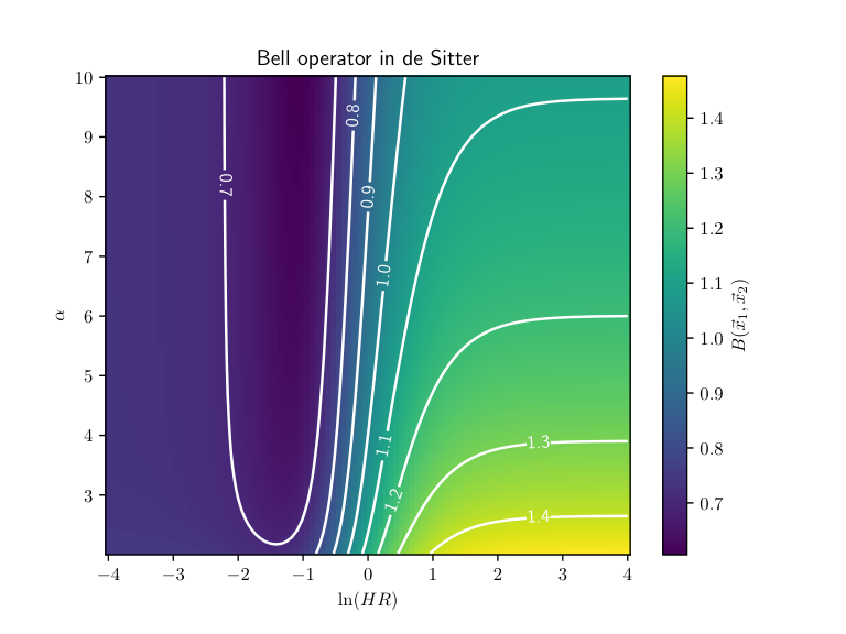
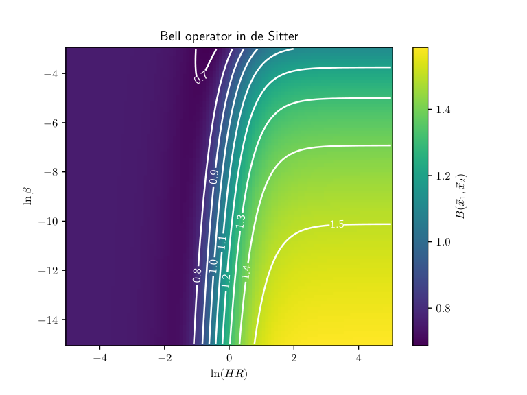
By plugging the covariance matrix (4.4) into the formulas of Sec. 2.4, the expectation value of the Bell operator can be computed, and the result is displayed in Fig. 3. In that figure, the UV and IR regulators have been respectively set to $\delta=10^{-2}$ and $\beta=10^{-4}$. Since there is at most a logarithmic dependence of the result on these parameters, they do not play a crucial role, and Fig. 3 rather shows how the result depends on $HR$ and $\alpha$ (see however Appendix C for figures displaying the dependence of $B$ on $\delta$ and $\beta$). One can see that two regimes need clearly to be distinguished, depending on whether $HR\ll 1$ (i.e. the size of the patches is smaller than the Hubble radius) or $HR\gg 1$ (i.e. the patches are larger than the Hubble radius).

When $HR\ll 1$, the result seems to carry little dependence on $\alpha$, and coincides with the values obtained in the left panel of Fig. 2 in the Minkowski vacuum. This is because, when $HR\ll 1/\alpha$, all distances involved in the problem (namely $R$ and $d$) are smaller than the Hubble radius, hence the setup is equivalent to a local Minkowski background. This is why the results of Sec. 3 are recovered in this regime, which can be formally verified by expanding the above formulas in $HR$ and then in $\alpha^{-1}$, leading to

In these expressions, $\gamma_{\mathrm{E}}$ is Euler’s constant, and the result is further expanded in $\delta$ and $\beta$. One thus recovers Eq. (3.6), with corrections suppressed by $(HR)^{2}$.

If $1/\alpha\ll HR\ll 1$, $R$ is smaller than the Hubble radius but not $d$, hence the flat space-time result may be modified a priori. However, this regime cannot be seen in Fig. 3 since it does not display large-enough values of $\alpha$. This is why, in Fig. 4, the expectation value of the Bell operator is shown as a function of $\alpha$, where $\beta$ and $\delta$ are fixed to the same value as in Fig. 3, and where we have set $HR=10^{-2}$. For comparison, the flat space-time result is also displayed. No strong deviation from the de-Sitter result can be observed, even when $d$ is larger than the Hubble radius. In any case, one can see that $B$ decreases with $\alpha$. Therefore, when $HR\ll 1$, $B$ is maximal in the Minkowski limit, where we have already shown that there is no Bell-inequality violation.

When $HR\gg 1$, one can see in Fig. 3 that an asymptotic value is also reached, which decreases with $\alpha$. This can be understood analytically by performing a large $HR$, large $\alpha$ expansion of the above formulas, which leads to

The conclusion of this analysis is that the configuration leading to the maximum expectation value for the Bell operator is the one where $HR$ is large and $\alpha$ is close to its minimum value. This corresponds to the situation where the coarse-graining scale $R$ is large compared to the Hubble radius, and the two patches are almost adjacent. In Appendix C, we further show that decreasing $\delta$ and $\beta$ make $B$ larger. This allows us to derive an upper bound on $B$ as follows. Formally, when $\beta\to 0$, the integrals $\mathcal{K}_{-1}$ and $\mathcal{L}_{-1}$ logarithmically diverge, and in the limit $\delta\to 0$, $\mathcal{K}_{3}$ logarithmically diverges too. This behaviour is such that $\mathfrak{p}=\braket{\hat{\mathcal{S}}_{z}(\vec{x}_{1})\hat{\mathcal{S}}_{z}(\vec{x}_{2})}\propto 1/\ln(\beta\delta)\to 0$ in this limit, and such that the argument of the $\arctan$ function in Eq. (2.16) goes to a finite constant (that only depends on $\alpha$ if one further lets $HR\to\infty)$. This proves that $\braket{\hat{\mathcal{S}}_{z}(\vec{x}_{1})\hat{\mathcal{S}}_{z}(\vec{x}_{2})}<1$ in this limit, hence $B<2$, see Eq. (2.14), which therefore applies to the whole parameter space.

References

- [1] J.S. Bell, On the Einstein-Podolsky-Rosen paradox, Physics Physique Fizika 1 (1964) 195.
- [2] S.J. Freedman and J.F. Clauser, Experimental Test of Local Hidden-Variable Theories, Phys. Rev. Lett. 28 (1972) 938.
- [3] A.A. Starobinsky, Spectrum of relict gravitational radiation and the early state of the universe, JETP Lett. 30 (1979) 682.
- [4] V.F. Mukhanov and G.V. Chibisov, Quantum Fluctuations and a Nonsingular Universe, JETP Lett. 33 (1981) 532.
- [5] S.W. Hawking, The Development of Irregularities in a Single Bubble Inflationary Universe, Phys. Lett. B115 (1982) 295.
- [6] A.A. Starobinsky, Dynamics of Phase Transition in the New Inflationary Universe Scenario and Generation of Perturbations, Phys. Lett. B117 (1982) 175.
- [7] A.H. Guth and S.Y. Pi, Fluctuations in the New Inflationary Universe, Phys. Rev. Lett. 49 (1982) 1110.
- [8] J.M. Bardeen, P.J. Steinhardt and M.S. Turner, Spontaneous Creation of Almost Scale - Free Density Perturbations in an Inflationary Universe, Phys. Rev. D28 (1983) 679.
- [9] A.A. Starobinsky, A New Type of Isotropic Cosmological Models Without Singularity, Phys. Lett. B91 (1980) 99.
- [10] K. Sato, First Order Phase Transition of a Vacuum and Expansion of the Universe, Mon. Not. Roy. Astron. Soc. 195 (1981) 467.
- [11] A.H. Guth, The Inflationary Universe: A Possible Solution to the Horizon and Flatness Problems, Phys. Rev. D23 (1981) 347.
- [12] A.D. Linde, A New Inflationary Universe Scenario: A Possible Solution of the Horizon, Flatness, Homogeneity, Isotropy and Primordial Monopole Problems, Phys. Lett. B108 (1982) 389.
- [13] A. Albrecht and P.J. Steinhardt, Cosmology for Grand Unified Theories with Radiatively Induced Symmetry Breaking, Phys. Rev. Lett. 48 (1982) 1220.
- [14] A.D. Linde, Chaotic Inflation, Phys. Lett. B129 (1983) 177.
- [15] Planck collaboration, Planck 2018 results. X. Constraints on inflation, 1807.06211.
- [16] D. Campo and R. Parentani, Inflationary spectra and violations of Bell inequalities, Phys. Rev. D 74 (2006) 025001 [astro-ph/0505376].
- [17] J. Maldacena, A model with cosmological Bell inequalities, Fortsch. Phys. 64 (2016) 10 [1508.01082].
- [18] S. Choudhury, S. Panda and R. Singh, Bell violation in the Sky, Eur. Phys. J. C 77 (2017) 60 [1607.00237].
- [19] J. Martin and V. Vennin, Bell inequalities for continuous-variable systems in generic squeezed states, Phys. Rev. A 93 (2016) 062117 [1605.02944].
- [20] J. Martin and V. Vennin, Obstructions to Bell CMB Experiments, Phys. Rev. D 96 (2017) 063501 [1706.05001].
- [21] S. Kanno and J. Soda, Infinite violation of Bell inequalities in inflation, Phys. Rev. D 96 (2017) 083501 [1705.06199].
- [22] L. Henderson and V. Vedral, Classical, quantum and total correlations, 0105028.
- [23] H. Ollivier and W.H. Zurek, Quantum Discord: A Measure of the Quantumness of Correlations, Phys. Rev. Lett. 88 (2001) 017901.
- [24] E.A. Lim, Quantum information of cosmological correlations, Phys. Rev. D 91 (2015) 083522 [1410.5508].
- [25] J. Martin and V. Vennin, Quantum Discord of Cosmic Inflation: Can we Show that CMB Anisotropies are of Quantum-Mechanical Origin?, Phys. Rev. D 93 (2016) 023505 [1510.04038].
- [26] T.J. Hollowood and J.I. McDonald, Decoherence, discord and the quantum master equation for cosmological perturbations, Phys. Rev. D 95 (2017) 103521 [1701.02235].
- [27] J. Martin, A. Micheli and V. Vennin, Discord and Decoherence, 2112.05037.
- [28] M. Revzen, P.A. Mello, A. Mann and L.M. Johansen, Bell’s inequality violation with non-negative Wigner functions, Phys. Rev. A 71 (2005) 022103 [quant-ph/0405100].
- [29] J. Martin, Cosmic Inflation, Quantum Information and the Pioneering Role of John S Bell in Cosmology, Universe 5 (2019) 92 [1904.00083].
- [30] K. Banaszek and K. Wódkiewicz, Testing quantum nonlocality in phase space, Phys. Rev. Lett. 82 (1999) 2009.
- [31] Z.-B. Chen, J.-W. Pan, G. Hou and Y.-D. Zhang, Maximal violation of bell’s inequalities for continuous variable systems, Phys. Rev. Lett. 88 (2002) 040406.
- [32] G. Gour, F.C. Khanna, A. Mann and M. Revzen, Optimization of Bell’s inequality violation for continuous variable systems, Physics Letters A 324 (2004) 415 [quant-ph/0308063].
- [33] J.-Å. Larsson, Bell inequalities for position measurements, Phys. Rev. A 70 (2004) 022102 [quant-ph/0310140].
- [34] L. Espinosa-Portalés and J. García-Bellido, Entanglement entropy of Primordial Black Holes after inflation, Phys. Rev. D 101 (2020) 043514 [1907.07601].
- [35] L. Espinosa-Portalés and J. García-Bellido, Long-range enhanced mutual information from inflation, Phys. Rev. D 103 (2021) 043537 [2007.02828].
- [36] J. Martin and V. Vennin, Real-space entanglement of quantum fields, Phys. Rev. D 104 (2021) 085012 [2106.14575].
- [37] P. Giorda and M.G.A. Paris, Gaussian Quantum Discord, Phys. Rev. Lett. 105 (2010) 020503 [1003.3207].
- [38] M.J.P. Morse, Statistical Bounds on CMB Bell Violation, 2003.13562.
- [39] J.F. Clauser, M.A. Horne, A. Shimony and R.A. Holt, Proposed experiment to test local hidden variable theories, Phys. Rev. Lett. 23 (1969) 880.
- [40] J. Martin and V. Vennin, Real-space entanglement in the Cosmic Microwave Background, 2106.15100.
- [41] H. Weyl, Quantenmechanik und Gruppentheorie, Zeitschrift fur Physik 46 (1927) 1.
- [42] H.J. Groenewold, On the principles of elementary quantum mechanics, Physica 12 (1946) 405.
- [43] J.E. Moyal and M.S. Bartlett, Quantum mechanics as a statistical theory, Proceedings of the Cambridge Philosophical Society 45 (1949) 99.
- [44] T. Colas, J. Grain and V. Vennin, Four-mode squeezed states: two-field quantum systems and the symplectic group , Eur. Phys. J. C 82 (2022) 6 [2104.14942].
- [45] H. Kodama and M. Sasaki, Cosmological Perturbation Theory, Prog. Theor. Phys. Suppl. 78 (1984) 1.
- [46] T.S. Bunch and P.C.W. Davies, Quantum Field Theory in de Sitter Space: Renormalization by Point Splitting, Proc. Roy. Soc. Lond. A 360 (1978) 117.
- [47] Planck collaboration, Planck 2018 results. X. Constraints on inflation, Astron. Astrophys. 641 (2020) A10 [1807.06211].
- [48] M.M. Dorantes and J.L. Lucio M, Generalizations of the pseudospin operator to test the Bell inequality for the TMSV state, Journal of Physics A Mathematical General 42 (2009) 285309.
- [49] J.P. Paz and G. Mahler, Proposed test for temporal Bell inequalities, Physical Review Letters 71 (1993) 3235.
- [50] C. Brukner, S. Taylor, S. Cheung and V. Vedral, Quantum Entanglement in Time, arXiv e-prints (2004) quant [quant-ph/0402127].
- [51] T. Fritz, Quantum correlations in the temporal Clauser-Horne-Shimony-Holt (CHSH) scenario, New Journal of Physics 12 (2010) 083055 [1005.3421].
- [52] A.J. Leggett and A. Garg, Quantum mechanics versus macroscopic realism: Is the flux there when nobody looks?, Phys. Rev. Lett. 54 (1985) 857.
- [53] J.S. Bell, EPR Correlations and EPW Distributions, Annals of the New York Academy of Sciences 480 (1986) 263.
- [54] J. Martin and V. Vennin, Leggett-Garg Inequalities for Squeezed States, Phys. Rev. A 94 (2016) 052135 [1611.01785].
- [55] K. Ando and V. Vennin, Bipartite temporal Bell inequalities for two-mode squeezed states, Phys. Rev. A 102 (2020) 052213 [2007.00458].
- [56] D. Green and R.A. Porto, Signals of a Quantum Universe, Phys. Rev. Lett. 124 (2020) 251302 [2001.09149].
- [57] R. Howl, V. Vedral, D. Naik, M. Christodoulou, C. Rovelli and A. Iyer, Non-Gaussianity as a signature of a quantum theory of gravity, PRX Quantum 2 (2021) 010325 [2004.01189].