Gravitomagnetic interaction of a Kerr black hole with a magnetic field as the source of the jetted GeV radiation of gamma-ray bursts
Abstract
We show that the gravitomagnetic interaction of a Kerr black hole (BH) with a surrounding magnetic field induces an electric field that accelerates charged particles to ultra-relativistic energies in the vicinity of the BH. Along the BH rotation axis, these electrons/protons can reach energies of even thousands of PeV, so stellar-mass BHs in long gamma-ray bursts (GRBs) and supermassive BHs in active galactic nuclei (AGN) can contribute to the ultrahigh-energy cosmic rays (UHECRs) thorough this mechanism. At off-axis latitudes, the particles accelerate to energies of hundreds of GeV and emit synchrotron radiation at GeV energies. This process occurs within around the BH rotation axis, and due to the equatorial-symmetry, it forms a double-cone emission. We outline the theoretical framework describing these acceleration and radiation processes, how they extract the rotational energy of the Kerr BH and the consequences for the astrophysics of GRBs.
Keywords:
gamma-ray bursts: general – black hole physics – pulsars: general – magnetic fieldsI Introduction
In the absence of any observational evidence, the process of gravitational collapse was studied in the simplest possible mathematical solution of the Einstein equations, i.e., for a spherically symmetric and vacuum spacetime (Oppenheimer & Snyder 1939; Finkelstein 1958; Kruskal 1960). The renaissance of the physics of general relativity started with the new era of relativistic astrophysics heralded by three discoveries:
- 1.
On June , , the first evidence of an X-ray source outside the solar system, Sco X1 (Giacconi et al. 1962), whose nature as a binary system was then identified by Shklovskii 1968. This was the first source of a long number of binary X-ray sources later discovered (Giacconi & Ruffini 1978, see, e.g.,). The identification of the detailed nature of Sco X1 stills today represents an open problem (Jia et al. 2020, see, e.g.,).
- 2.
On July , , the discovery by Kerr 1963 of an algebraically-special metric, among the solutions of the Einstein field equations in vacuum, that describes the gravitational field of a spinning mass. The Kerr solution introduced a theoretical formalism of unprecedented complexity in general relativity to describe the effect of the rotation in the black hole (BH) geometry. From an observational point of view, the Kerr metric offered, in principle, since 1971 (see below) an unprecedented energy source for an astrophysical system, alternative, e.g., to nuclear energy sources.
- 3.
On March , , the epochal discovery of the quasar nature of the radio source 3C 273 by Schmidt 1963, at , i.e., at a distance of about Mpc, implying energies of erg originating from the nuclear region of a galaxy. The explanation of the energy source in terms of the rotational energy of the BH is among the leading open astrophysical problems still today, and gaining additional crucial observations from closer AGN as M87 at (Bird et al. 2010) and IC 310 at (Bernardi et al. 2002).
The authentic shock of the pulsar discovery, the very quick identification of its nature as the first observed gravitationally collapsed object, and the long awaited explanation of the nature of the supernova (SN), marked the real birth of relativistic astrophysics and of the physics of gravitational collapse. The discovery of the Crab Nebula pulsar by Hewish et al. 1968 allowed:
- 1.
The first, unequivocal observational identification of a pulsar as a rapidly rotating NS (Gold 1968; Pacini 1968; Finzi & Wolf 1969).
- 2.
The possibility to confirm the hypothesis of Baade & Zwicky 1934 that NSs originate in SNe. In this case, the Crab pulsar had originated in the SN observed by Chinese astronomers in the year (Shklovskii 1953; Shklovskij 1969).
- 3.
To conceptually realize that, the process of gravitational collapse leading to NS formation is not an isolated event in time, but followed by a long-lasting emission of thousands of years. The conceptual role of this prolonged emission, traditionally neglected, is now acquiring a special role in the context of gamma-ray bursts (GRBs), where both the collapse to a NS and to a BH are observed daily with a long lasting X-ray and GeV emission (see Ruffini et al. 2021, references therein, and Eqs. 1–2 in this article).
In Princeton, John A. Wheeler’s group proceeded ahead in the study of BHs adopting as a background the geometry of the Kerr solution. This research program soon materialized in three steps:
- 1.
The introduction in of the effective potential technique to determine the properties of co-rotating and counter-rotating orbits, including the often quoted last stable circular orbits in the Kerr metric (see Ruffini & Wheeler in §104 of Landau & Lifshitz 1975).
- 2.
The identification, among these trajectories, of the ones corresponding to reversible and irreversible transformations presented in Christodoulou 1970. The derivation by Demetrios Christodoulou of the mass-energy formula of a Kerr BH was made possible by introducing the concept of irreducible mass (from the Italian “irriducibile”) following the definition of ergosphere introduced in Christodoulou 1970 by Ruffini and Wheeler. The further relation between the irreducible mass and the horizon area was soon shown in Christodoulou & Ruffini 1971 and Hawking 1971. These results were obtained practicing on the gedanken “Penrose process”, see Fig. in Christodoulou 1970, which we found to be physically not implementable, as confirmed later by Penrose & Floyd 197111 1 The negative results on the “Penrose process” have in no way affected the derivation of the irreducible mass, uniquely based on the reversible and irreversible transformations, which never attracted Penrose’s attention..
- 3.
The publication of “Introducing the black hole” (Ruffini & Wheeler 1971a), where the BH was introduced as a physical system characterized by three parameters, the total mass, , the angular momentum, , and the irreducible mass, , with the geometry given by the Kerr metric.
A first step in this novel domain established the absolute upper limit to the value of the critical mass of a non-rotating NS, , generalizing the first established value of by Oppenheimer & Volkoff 1939. The result was obtained, out of first principles, imposing the non-violation of causality, a fiducial nuclear density, and adopting the validity of general relativity (Rhoades & Ruffini 1974). A second step was the discovery of the first BH in our galaxy, Cygnus X1 (Leach & Ruffini 1973; Ruffini 1974; Giacconi 2003), using X-ray and optical data and imposing the above critical mass limit for BH formation. Nevertheless, the discovery of such a Galactic object, although of great interest, did not offer any evidence for the new physics of the irreducible mass. It was clear that a binary X-ray source evolves on a timescale of yr, so we initially thought that we would have to wait for too long to see what occurs next in their evolution. But this was a big mistake. The gravitational collapse releases about erg, so such an event would be visible from any place in the Universe, and from the number of binary X-ray sources, that would lead to the observation of these events almost everyday. We had to wait a third gigantic step following the launch of Beppo-Sax and the discovery of the extragalactic origin of GRBs (Costa et al. 1997; van Paradijs et al. 1997). It was then started an unprecedented experimental effort of observing these most unique sources in the vastest range of wavelengths, from the radio to the keV, to the MeV, to the GeV, to the TeV, to the ultrahigh-energy cosmic rays (UHECRs). As a result, we have the opportunity to observe these sources up to high values of the cosmological redshift, e.g. , allowing us to witness on a daily basis the birth of NSs and BHs. This new unprecedented condition allows us, for the first time, to submit also our own theoretical analysis to the scrutiny of direct observations and to verify which one of our theoretical assumptions, introduced years ago, were made just for the sake of simplicity or mathematical convenience.
In parallel, a novel path of theoretical research was gaining attention, diverging from a pure gravitational analysis of an isolated BH, in vacuum and stationary. Interest was called on the electrodynamics and magneto-hydrodynamics around BHs and on BH gravito-hydrodynamics (see Punsly 2009, and references therein). The BH theory based on the above theoretical developments and on the vastest multiwavelength observations has been started to be constructed,¡ with necessary changes of paradigm, and new ones that we infer in this article.
This article is dedicated to the development of the theoretical framework of the “inner engine” originating the GeV radiation of GRBs within the binary-driven hypernova (BdHN) scenario (see Ruffini et al. 2019b, references therein, and Sec. II for details). It emphasizes the special role of the interaction of the gravitomagnetic field of a Kerr BH with a uniform, asymptotically aligned background test magnetic field, following the mathematical solution of the Einstein-Maxwell equations by Papapetrou 1966 and Wald 1974, hereafter referred to as the Papapetrou-Wald solution (see Secs. III–VI for details). As we shall shown, the above leads to a mechanism of particle acceleration and radiation in the BH vicinity, leading to UHECRs along the BH rotation axis, and to GeV radiation at off-axis latitudes within of the polar axis, with equatorial symmetry, i.e. there is a double-cone emission structure. The theory equations and their solution describing the particle acceleration and radiation processes, how they extract the rotational energy of the Kerr BH, as well as the consequences for the astrophysics of GRBs and AGN are here outlined.
The article is organized as follows. In Sec. II, we outline the observational features of the formation of a Kerr BH in a BdHN of type I, using GRB 190114C as a prototype. Section III describes the structure of the electromagnetic field of the Papapetrou-Wald solution. In Sec. III, we present the general relativistic equations of motion for charged particles including radiation losses. We show in Sec. IV specific results of the numerical integration of the equations of motion. In Sec. V, we analyze the properties of the photon four-momentum observed at infinity to infer the properties of the observed radiation. Section VI is devoted to give quantitative estimates of the radiation power and the spectrum. Finally, we present in Sec. VII our conclusions.
II Black hole formation in a BdHN I: GRB 190114C as a prototype
Prior to the year , GRBs were traditionally considered as single objects originating their energy from a Kerr BH (Rees & Meszaros 1992; Woosley 1993; Piran 1999, see, e.g.,). Since then, a new scenario has been gradually developing in which GRBs originate in binary systems leading to their classification in nine GRB subclasses (Ruffini et al. 2016; Wang et al. 2019; Rueda et al. 2020, see, e.g.). What has become clear is that a BH is generated only in some short GRBs originating in NS-NS mergers, and only in some long GRBs originating in binaries composed of a carbon-oxygen (CO) star and a NS companion in tight orbit.
We now focus on the latter special subclass of long GRBs that originate in short-period CO-NS binaries. The GRB ignition works as follows. As the CO star gravitationally collapses, it gives origin to a SN explosion and to a new NS (hereafter NS) at its center. The ejected matter in the SN produces a hypercritical (i.e. highly super-Eddington) accretion process both onto the NS (via matter fallback) and onto the companion NS. For short orbital periods of the order of a few minutes, the accretion process onto the NS companion is sufficiently massive to lead it to the critical mass, hence forming a BH (see Fig. 1). We have called these systems BdHN of type I (Wang et al. 2019, see, e.g.,). Until now, of BdHN I have been identified, with their evolution following a precise sequence of episodes, which we now indicate using GRB 190114C as a prototype (Moradi et al. 2021b; Moradi et al. 2021a).


The time coincides with the trigger of GRB 190114C given by the Fermi satellite. The progenitor is a CO-NS binary with an inferred orbital period of min (Rueda et al. 2020). The appearance of the NS, hereafter NS-rise (formerly called SN-rise), following the CO star core-collapse, occurs between s and s in the rest-frame of the source. The NS-rise triggers the entire BdHN I evolution. In the SN explosion, as usual, a NS is created, which operates in addition to the binary companion NS (see Fig. 1). The spectrum of the NS-rise, observed in the gamma-rays by the Fermi-GBM detector, is shown in Fig. 2 (upper left panel). The energy of the NS-rise in GRB 190114C is erg (Ruffini et al. 2021).
The SN ejecta now accrete at hypercritical rates onto the binary companion NS. At s, the NS companion reaches its critical mass and collapses creating a Kerr BH, highlighted by the onset of the GeV emission (see Fig. 2; lower left panel). Between s and s in the source rest-frame, the ultrarelativistic prompt emission (UPE) occurs, characterized by a cutoff power-law plus blackbody (CPL + BB) spectrum and the energetics reported in Fig. 2 (upper right panel). The energy released observed in the UPE phase is erg (Moradi et al. 2021b).
At s, the turn on of the Neil Gehrels Swift satellite occurs and allows to perform the observations of the ongoing emission of the X-ray afterglow. One of the major successes of the BdHN I theory has been the identification in the SN accretion onto the rapidly rotating NS, with a spinning period of ms (Rueda et al. 2020), the energy source of the afterglow of GRB 190114C (see Fig. 2; lower right panel). The observations of GRB 190114C and of its “twin” source GRB 180427A have further allowed to explain the observed spectra of the afterglow characterized by the synchrotron emission originating from the rapidly rotating NS, interacting with the SN ejecta. Further examples of afterglows fulfilling this approach and leading to the determination of the NS rotation period have been the cases of GRB 180728A with a NS spin of ms, GRB 130427A with ms, GRB 160625B with ms, GRB 160509A with ms, and GRB 090926A with ms (Rueda et al. 2020).
A most significant result has been that all identified BdHN I have an afterglow characterised by a decreasing luminosity with time, that expressed in the rest frame of the source is well fitted by a power-law function
| (1) |
which for GRB 190114C erg s-1 and (Ruffini et al. 2021). The observed energy released in the X-ray emission is erg.
We have identified above the role of the SN in creating a magnetized rapidly rotating NS, as well as its role in producing a hypercritical accretion process onto the NS which helps to power the X-ray afterglow. There are three main conclusions on the afterglow:
- 1.
The initial rotational energy of the NS with the observed power-law luminosity given by Eq. (1) may well justify an afterglow emission occurring for an infinite time.
- 2.
These results open a new scenario with respect to the usually assumed ultrarelativistic blastwaves in the traditional GRB model, which has been shown to contradict model-independent constraints (Ruffini et al. 2018) and implying unacceptable energetic requirements for the system.
- 3.
The presence of a rapidly spinning NS in the afterglow can lead to the possibility of relating NS “glitches” to the emission of TeV emission, e.g. in GRB 180720B (Moradi, et al., submitted).
At s, at the end of the UPE phase, the GeV radiation observed by LAT is emitted following a decreasing power-law luminosity (see Fig. 2; lower left panel)
| (2) |
with erg s-1 and . The energy of the GeV emission is erg (Moradi et al. 2021a).
The existence of the above mentioned power-laws in the X-ray emission observed by the Swift satellite, originating from the rotational energy extraction from a spinning NS, see Eq. (1), and the analogous one in the GeV observed by the Fermi-LAT satellite, originating from the rotational energy extraction Kerr BH, see Eq. (2), are the two conceptually new observables characterizing GRBs. Every gravitational collapse episode occurring within a GRB, either leading to a rotating NS or to a rotating BH, is not an isolated event in space and time. On the contrary, it is the beginning of a process characterized by a decreasing power-law luminosity that, in principle, may last the entire life of the Universe. What is clear is that, currently, we are observing all alive Kerr BHs and not dead Schwarzschild BHs. The crucial characterization of this difference resides in the jetted emission and the possible presence of trapped surface and of shadows cannot be meaningfully addressed on the ground of this physics.
In order to approach in the following sections the physics of the inner engine, we have first to introduce three main new paradigms:
- 1.
The rotational energy extraction from a Kerr BH and the associated acceleration process originates in the gravitomagnetic interaction of the Kerr BH with a uniform background magnetic field (Ruffini et al. 2019b). Necessarily, the conditions of stationarity of the Kerr solution, as well as assuming such a solution in vacuum and all the considerations of the geodesics of uncharged particles have to be superseded, see Sec. III.
- 2.
The geodesic equations of motion of massive particles around a Kerr BH (Ruffini & Wheeler 1971b; Ruffini & Wheeler 1971a) are superseded by the equation of motion of positively and negatively charged particles in the field of a Papapetrou-Wald solution, taking into due account the radiation reaction forces; see Secs. IV and V, as well as Appendix A–C.
- 3.
III The electromagnetic field structure
The inner engine of the high-energy emission of long GRBs was presented in Ruffini et al. 2019b, and applied there to GRB 130427A. It is composed of a Kerr BH (Boyer & Lindquist 1967; Carter 1968), embedded in a test, asymptotically aligned magnetic field, described by the Papapetrou-Wald (Papapetrou 1966; Wald 1974) solution of the Einstein-Maxwell equations.
We here present a full (numerical) integration of the equations of motion of a charged particle in the electromagnetic field of the Papapetrou-Wald solution, accounting for radiation in the background of the Kerr metric. We use geometric units , unless otherwise specified.
Denoting by and , respectively the time-like and space-like Killing vectors for the Kerr metric (see Appendix A), the electromagnetic four-potential is given by (Wald 1974)
| (3) |
where is the asymptotic value of the magnetic field strength. Because of and , the non-vanishing components of the four-potential, in the Boyer-Lindquist coordinate basis of the Kerr metric (see Appendix A), read
| (4) | ||||
| (5) |
As in Damour et al. 1978, we introduce a local Lorentz observer, specifically a locally non-rotating (LNR) observer (Bardeen 1970; Bardeen et al. 1972), in order to analyze the electromagnetic field properties and the equations of motion.
The LNR observer carries a tetrad basis with vectors ; see Appendix A for details on the tetrad and related framework of the subsequent calculations. We use a hat to distinguish components (projections) in the LNR frame from the ones in coordinate frame. Latin alphabet (e.g. ) and Greek indexes (e.g. ) run over the spacetime coordinates, i.e. from to (, , , and ), while Latin indexes (e.g. ) run only over the spatial coordinates.
In the LNR frame, the electric and magnetic field components are given by
| (6a) | ||||
| (6b) | ||||
where is the electromagnetic field tensor in the coordinate basis. Expressed in Boyer-Lindquist coordinates, the electric and magnetic field are (Damour et al. 1978)
| (7a) | ||||
| (7b) | ||||
| (8a) | ||||
| (8b) | ||||
For completeness, we give the expressions of the electric and magnetic field in the Boyer-Lindquist coordinate basis (see Eqs. B2)
| (9a) | ||||
| (9b) | ||||
Figures 3 and 4 show the electric and magnetic field lines as seen by the LNR observer, in the - plane in Kerr-Schild coordinates (see Appendix A). We describe now the physical situation in the northern hemisphere since because of the equatorial symmetry, the situation in southern hemisphere will be exactly the same. Electrons move outwardly where the electric field is inwardly directed. Clearly, the opposite happens for protons, they move outwardly where the electric field is outwardly directed. In Fig. 3, we show the case of an asymptotically parallel magnetic field to the BH spin. The electric field is inwardly directed in the cone of semi-aperture angle from the polar axis. Therefore, in this situation we have a polar electronic jet. At , the electric field vanishes and reverse direction, i.e. the electric field becomes outwardly directed. In Fig. 4, we show the case of an asymptotically antiparallel magnetic field to the BH spin. In this case, the electric field is outwardly directed in the cone of semi-aperture angle from the polar axis, creating a polar electronic jet.

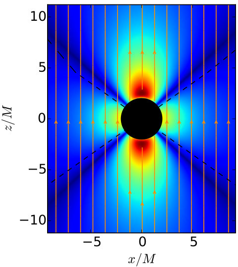
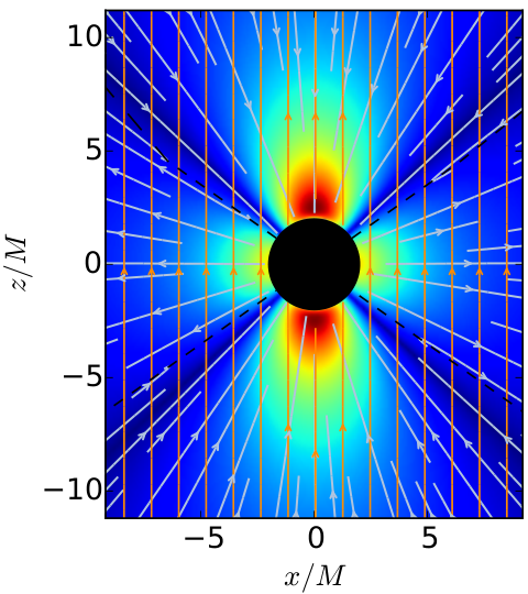


For moderate spin values (i.e. ), the electric and magnetic fields are accurately represented by the lowest order of their expansions in the dimensionless spin parameter , i.e. up to first order we have
| (10a) | ||||
| (10b) | ||||
| (10c) | ||||
| (10d) | ||||
We can see that within this approximation, the electric field reverses sign at , i.e. , in agreement with the full numerical result. It can be checked that the magnetic field is asymptotically directed along the -direction. Evaluating the Kerr-Schild components (see Appendix B), e.g. on the plane , we obtain
| (11a) | ||||
| (11b) | ||||
| (11c) | ||||
It is then clear that for radial distances , we have , , and . The dominance of the z-component actually occurs everywhere and for any value of the BH spin parameter , as it can be seen from Fig. 3 which shows the electric and magnetic field lines without any approximation.
The electric field (7) is induced by interaction of the magnetic field and the BH gravitomagnetic field. In fact, it is easy to check that it vanishes for . As we have seen in Figs. 3 and 4, the electric field has a quadrupolar nature. Thus, although the BH has a zero net charge, we can think of this field as produced by a quadrupolar distribution of charges of surface density (Thorne et al. 1986)
| (12) |
that in the slow rotation approximation becomes
| (13) |
From this expression it is clear that it equals , where the electric field is given by Eq. (10), as expected. From this expression, we have that the surface charge vanishes at , which leads to , consistent with the value already obtained directly from the electric field expression and shown in Figs. 3 and 4.
By introducing the dimensionless radius and the spin parameter in units of , it can be seen that the surface charge does not depend explicitly on , but only on and . Figure 5 shows the surface charge (12) as a function of , for a BH spin parameter , the same used in Fig. 3. This surface charge in fact agrees with the electric field lines in the upper row plots of Fig. 3. In the first patch, (the angle is measured clockwise from the polar axis), the electric field lines are inwardly directed as expected from ; the electric field lines in the region point outward in agreement with . A similar analysis for the other patches confirm the self-consistency of the scenario. The angle is the one for which vanishes. For this numerical example, .
We can compute the charge induced on a surface patch of the horizon as
| (14) |
where is the induced metric on the horizon, , being , and , obtained by taking constant slices and in the Kerr metric (A3). Therefore, Eq. (14) becomes
| (15) |
where we have already performed the integral over taking advantage of the axial symmetry and denotes the angular region subtended by two spherical polar angles. The integral in Eq. (15) from to vanishes, so the net charge of the BH is zero. In the example of Fig. 5, the charge of the negatively charged patches is obtained by summing the integrals in the regions and , while the positively charged one is obtained from the integral in the region . For the case of , we obtain
| (16) |
and therefore, , as expected.
We can obtain an analytic expression of the patch charge in the slow-rotation regime. By replacing given by Eq. (13) into Eq. (15), we obtain the charge on any patch
| (17) |
We can now evaluate the total negative and positive charge as we proceeded before, which leads us to
| (18) |
where in the last equality we have used the BH angular momentum via the relation . Turning to the previous numerical example, i.e. , Eq. (18) gives , which is pretty close to the value given by Eq. (16), validating once more the accuracy of the slow-rotation approximation.
IV Equations of motion
In the LNR frame, the particle equations of motion can be written as
| (19) |
where and and are, respectively, the components of the particle’s four-velocity and the electromagnetic field tensor, projected onto the observer’s tetrad, see Eqs. (B6) and (B5), is the particle’s proper time along its worldline, and are the spin coefficients given by Eqs. (B14) The last term on the right-hand side are the components of the radiation-reaction “force” (Landau & Lifshitz 1975, see, e.g.,) per unit mass, projected onto the LNR frame, i.e.
| (20) |
where in the last term the covariant derivative of the electromagnetic tensor in the LNR frame can be computed via Eq. (B12).
The radiation reaction force (IV) is largely dominated by the first term, hence
| (21) |
where we have defined the radiated off power
| (22) |
We can work in the slow-rotation regime which provides sufficient accuracy for our purpose. Within this approximation, Eqs. (19) become
| (23) |
and
| (25) |
where , and are given by their corresponding slow-regime expressions given by Eqs. (10).
It is worth to assess the relative importance of the purely gravitational terms in the dynamics of the particle. It is clear than the contribution of the square brackets on the right-hand side of Eq. (IV) is dominated by the first term inside them. Then, because of , the order of magnitude of the ratio between the electric field term and the gravitational one is given by , where is the so-called gyration angular frequency. Therefore, since the largest value of the spin parameter is , the largest value that the electric to gravitational contributions ratio can attain is , that becomes of the order of unity only for an extremely weak magnetic field of the order of G. This implies that, for a magnetic field G, the electric field term is bigger than the gravitational one. Only in the limit , the gravitational attraction can play some role against such a huge electric force. Therefore, we expect the evolution of to be dictated only by the first term on the right-hand side of Eq. (IV). A similar analysis can be done for the evolution of the spatial velocity, which we therefore expect to be fully dominated by the terms in the first row of Eq. (IV).
IV.1 A specific numerical solution
We turn now to show specific examples of numerical solutions to the equations of motion (IV) and (IV), for inner engine parameters: , , G (so rad s-1).
Figure 6 shows an example of the trajectory of an electron initially located at , , . The initial values of the electron’s velocity components were, in this specific example, were set to have a spiraling electron motion, that is setting up an initially dominating azimuthal velocity, in particular we have chosen , and , with . The trajectory is shown at times , when the spiraling behavior is better appreciated. At longer times, the electron follows closely the magnetic-field lines which are nearly -directed (see Fig. 3), so the z-component of the velocity becomes dominant (see also Fig. 7).
In Fig. 6, the position displacements in the and direction are in units of and the one in the direction in units of . Indeed, a dimensionless proper time corresponds to s, so the observer measures a displacement cm, for the chosen BH mass. The displacements in the - plane are smaller since the particle’s velocity is dominated by the -component.
Figure 7 shows the evolution of the position and velocity components of an electron located at , (upper row), (lower row) and . The electron has been set initially at rest, i.e. , so . This figure shows that, in general, the motion along the -direction is dominant, and it is even more pronounced for small spherical polar angles (motion nearly attached to the BH rotation axis).
V Photon four-momentum measured at infinity
We refer the reader to App. B for the general equations between the four-momentum measured by the observer at rest at infinity, the LNR observer and the comoving observer. We can gain some (analytical) insight into the features of the photon emission by assuming , and . In this one-dimensional approximation of motion, Eqs. (C6) reduce to
| (26a) | ||||
| (26b) | ||||
which in the slow-rotation regime can be written as
| (27a) | ||||
| (27b) | ||||
| (27c) | ||||
| (27d) | ||||
where we have introduced the notation . We have also parametrized the spatial components of the photon four-momentum in the orthonormal comoving frame as
| (28) |
where and are spherical polar and azimuth angles measured by this local observer. This choice satisfies , which derives from .
Thus, by assigning values to these angles in their corresponding range, i.e. and , we can compute from Eqs. (27) the corresponding normalized components of the photon four-momentum in the coordinate frame. Figure 8 compare and contrast the photon four-momentum components calculated with the general equations (C6) with the ones obtained from the approximate equations (27). In this example, the photons are emitted from the two positions of Fig. 7, and make angles and as measured by the comoving observer.
Table 1 shows the photon four-momentum components as measured by the observer at rest at infinity, i.e. , for photons emitted in the plane of the comoving observer (i.e. -), and in the plane (i.e. -), in the directions , , and .
| : plane - | : plane - | |||||
|---|---|---|---|---|---|---|
| 0 | 0 | 0 | ||||
| + | ||||||
It can be seen from the above equations (see also their summary in Table 1) that
- 1.
There is a purely general relativistic effect: the azimuthal photon four-momentum component, , has a contribution from the angular velocity associated with the frame-dragging effect. This contribution vanishes only for photons emitted by electrons accelerated along the BH rotation axis (). For off-axis motion, it does not vanish and it can be even larger than the polar component, (see Table 1 and Fig. 8).
- 2.
The above implies that relativistic aberration by which photons are measured at infinity as confined within an angle around the direction of motion of the emitter (Landau & Lifshitz 1975, see e.g.), strictly holds only along the BH rotation axis. However, the radial component of the four-momentum is still dominant and the traditional relativistic aberration can be assumed for practical purposes.
VI Radiation power and spectrum
The above result allows us to estimate the radiation by acceleration using known results from special relativity. Most of the synchrotron power is radiated around the peak of the spectrum which occurs near the characteristic angular frequency (Landau & Lifshitz 1975)
| (29) |
where is the relativistic curvature radius
| (30) |
The left panel of Fig. 9 shows electron Lorentz factor as a function of the dimensionless proper time, and the right panel the characteristic photon energy, . We show the results for three different initial conditions; the electron starts its motion at rest at , where , , and (blue curves), (green curves), and .
The electron reaches an asymptotic value when acceleration and radiation losses balance each other. At small values of the spherical polar angle, the electron experiences less radiation losses reaching a higher Lorentz factor and higher photon energy. Furthermore, the photon characteristic energy falls in the GeV regime at the asymptotic Lorentz factor. Therefore, most of the radiation is emitted at GeV energies.
We now turn to the energy distribution of the radiation. The synchrotron power radiated by an electron, per unit angular frequency , and integrated over the solid angle is (Landau & Lifshitz 1975, see, e.g.,)
| (31) |
where , and is the modified Bessel function of the second kind.
We plot in Fig. 10 the (bolometric) power radiated off at infinity (left panel), , as a function of dimensionless proper time. The obtained power per electrons shows that to emit, for instance, a luminosity of erg s-1, we must accelerate about electrons. Since the acceleration occurs in the proximity of the BH horizon, these electrons occupy a volume cm3, implying a number density cm-3. In fact, for the LNR observer the inner engine can accelerate the following number of electrons per unit volume
| (32) |
where is given by Eqs. (7). The electric field near the horizon is , where , so Eq. (32) gives . For the present quantitative example, so using (see Fig. 9), Eq. (32) gives cm-3, as expected from our previous estimate. The number of electrons around the Kerr BH can be either lower and higher than this value, but the inner engine can accelerate at most the above number of electrons. The density in the cavity created around the Kerr BH formed from the gravitational collapse of the NS in a BdHN is of the same order as the above value (see Becerra et al. 2019; Ruffini et al. 2019a, for numerical simulations). This implies that the inner engine in BdHNe works efficiently using its full energy reservoir.
The right panel of Fig. 10 shows the spectrum density, i.e. the radiated power per unit volume, , as a function of the photon energy (calculated as ). Here, is given by Eq. (32). This plot confirms that most of the energy is emitted in the GeV domain, and the above-mentioned value of the electron density of particles that can be accelerated, in fact erg s-1 cm-3.
Summarizing, the gravitomagnetic interaction of the Kerr BH with the surrounding magnetic field efficiently accelerate electrons from the ionized environment in the BH vicinity. This acceleration and radiation process emits photons in the GeV regime for magnetic fields in the – G and stellar-mass Kerr BHs. The emission originates in proximity of the BH horizon and within from the BH rotation axis with equatorial symmetry, hence generating a double-cone “jetted” high-energy (GeV) emission.
VII The black hole energy extraction
It is clear that the energy radiated off to infinity must necessarily come from the BH extractable energy
| (33) |
where the total mass is given by the BH mass-energy formula (Christodoulou 1970; Christodoulou & Ruffini 1971; Hawking 1971)
| (34) |
where , , are respectively the angular momentum and the mass of the BH.
In order to understand better how the BH rotational energy is extracted, it is useful to recall the inner engine operation:
- 1.
- 2.
The induced electric field accelerates electrons outwardly. The number of electrons that can be accelerated is set by the energy of the electric field
(35) where we have used Eq. (10).
- 3.
The maximum possible electron acceleration/energy is set by the electric potential energy difference from the horizon to infinity
(36) - 4.
Along the polar axis, radiation losses by acceleration are absent because the electric and magnetic fields are parallel. Therefore, electrons accelerated on the BH rotation axis can gain the full potential energy difference (36).
- 5.
At off-axis latitudes, the accelerated electrons emit synchrotron radiation. In order to explain the observed luminosity, , the radiation timescale, , must fulfill
(37) where is given by Eq. (35), and we assume most of this energy is radiated off in high-energy photons, as we have shown in Sec. VI. We take here into account that the energy reservoir is the rotational energy of the BH, therefore, the extractable energy must satisfy
(38) where is given by Eq. (33) and is the energy observed at high-energies, i.e.:
(39) - 6.
Once the energy has been emitted, the BH is left with new values of mass and angular momentum which have been reduced by amounts and , respectively. The change in the BH mass is
(40) According to the BH mass-energy formula (34), if in the energy extraction process the irreducible mass is kept constant, the change in the BH angular momentum is
(41) - 7.
The above steps are repeated, with the same efficiency, if the density of plasma is sufficient, namely if the number of the particles is enough to cover the new electric energy. Therefore, the inner engine evolves in a sequence of elementary processes, each emitting a well-defined, precise amount of BH rotational energy.
Therefore, the total fractional changes of mass and angular momentum in the whole emission process are
| (42) | ||||
| (43) |
where we have used Eqs. (34), (40), (41), and the relation between the BH irreducible mass and the horizon:
| (44) |
As a quantitative example, let us use our present fiducial parameters G, and . In this case, the electric energy is erg. The radiated luminosity is set by the timescale at which is radiated off. Figures 9 and 10 show that electrons reach a Lorentz factor , so an energy of nearly erg, which is then radiated off at a rate erg s-1, leading to a radiation timescale
| (45) |
of the order of s. We recall that is the four-momentum of the particle measure by an observer at rest at infinity and is the time-like Killing vector. This estimate of the timescale is confirmed by Fig. 11 which shows the time evolution of . This radiation timescale implies that the system radiates off with a power erg s-1. This energy is mainly radiated at photon of energies of the order of GeV (see right panels of Figs. 9 and 10).
For these parameters, in each elementary emission, the BH mass and angular momentum experience fractional changes , and , respectively. The BH irreducible mass can be readily obtained from Eq. (44), i.e. . Therefore, the total extractable energy is erg. If is emitted, the total fractional changes in the BH mass and angular momentum will be, respectively, and .
VIII Discussion and Conclusions
Summarizing, all BdHN I are powered by three independent sources of energy:
- 1.
The BdHN I is triggered by the NS-rise produced in the core-collapse of the CO star generating a NS at its center. The NS rotational energy powers the synchrotron emission from the expanding SN that originates the X-ray afterglow (see Rueda et al. 2020, and references therein).
- 2.
The hypercritical accretion of the SN material onto the binary companion NS leads to the formation of the BH when it reaches the critical mass for gravitational collapse (Becerra et al. 2016; Becerra et al. 2019, see, e.g.). This “smooth” accretion leading to BH formation does not emit any detectable signal of gravitational waves and is alternative to the direct gravitational collapse of a massive star (collapsar).
- 3.
The gravitomagnetic interaction of the Kerr BH with the surrounding magnetic field, in presence of ionized matter of the SN ejecta, leads to the process of extraction of the BH rotational energy, generating the “jetted” high-energy (GeV) emission. We have here shown that this radiation is emitted in the vicinity of the BH horizon within from the BH rotation axis (see Secs. II and VI).
We have focused in this article on the inner engine of the high-energy emission, which as we have shown drives a new paradigm in the theory of GRBs:
- 1.
There is no need for bulk motion. The traditional GRB model uses the gravitational pull to accelerate matter in bulk up to very large distances – cm, where the ultrarelativistic blastwave becomes transparent to high-energy photons. The inner engine, instead, radiates at horizon scales the kinetic energy rapidly gained by single-particle acceleration (Secs. III–VI). As shown in Moradi et al. 2021a; Ruffini et al. 2019b, the radiated high-energy photons are transparent to magnetic pair production, likely the most important opacity source of this system.
- 2.
There is no need of massive accretion. The density of ionized matter needed for the inner engine to explain the GeV emission of a long GRB is much lower than the corresponding one requested by traditional matter accretion. For example, an accretion disk produces a luminosity , where is a parameter accounting for the efficiency in converting gravitational energy into radiation. Adopting a fiducial value , in order to get a luminosity of erg s-1, the BH must accrete matter at a rate s-1. This implies a consumption of protons by the BH at a rate of s-1, or a proton number density rate cm-3 s-1. Clearly, smaller values of require larger accretion rates. The inner engine, instead, produces the same luminosity by accelerating electrons with a rate s-1, i.e. s-1 (for fully ionized matter), or an electron density of cm-3 s-1; see discussion of Eq. (32) in Sec. VI for further details. This implies that the geodesic equations of motion of massive particles around a Kerr BH, traditionally applied to the problem of gravitational matter accretion, are superseded by the equation of motion of charged particles, accounting for the radiation reaction, accelerated in the electromagnetic field of the Papapetrou-Wald solution (see Secs. IV–VI).
- 3.
The BH is responsible only for the high-energy radiation. During the acceleration region, the electrons radiate mainly at high-energies, e.g. GeV (see Sec. VI). The fundamental role of the reversible transformations holds. Indeed, the energy budget is paid by the BH extractable energy (Rueda & Ruffini 2020), and the irreducible mass of the BH mediates the energy extraction process (see Sec. VII).
References
- Baade & Zwicky (1934) Baade, W., & Zwicky, F. 1934, Physical Review, 46, 76, doi: 10.1103/PhysRev.46.76.2
- Bardeen (1970) Bardeen, J. M. 1970, ApJ, 162, 71, doi: 10.1086/150635
- Bardeen et al. (1972) Bardeen, J. M., Press, W. H., & Teukolsky, S. A. 1972, ApJ, 178, 347, doi: 10.1086/151796
- Becerra et al. (2016) Becerra, L., Bianco, C. L., Fryer, C. L., Rueda, J. A., & Ruffini, R. 2016, ApJ, 833, 107, doi: 10.3847/1538-4357/833/1/107
- Becerra et al. (2019) Becerra, L., Ellinger, C. L., Fryer, C. L., Rueda, J. A., & Ruffini, R. 2019, ApJ, 871, 14, doi: 10.3847/1538-4357/aaf6b3
- Bernardi et al. (2002) Bernardi, M., Alonso, M. V., da Costa, L. N., et al. 2002, AJ, 123, 2990, doi: 10.1086/340463
- Bird et al. (2010) Bird, S., Harris, W. E., Blakeslee, J. P., & Flynn, C. 2010, A&A, 524, A71, doi: 10.1051/0004-6361/201014876
- Boyer & Lindquist (1967) Boyer, R. H., & Lindquist, R. W. 1967, Journal of Mathematical Physics, 8, 265, doi: 10.1063/1.1705193
- Carter (1968) Carter, B. 1968, Physical Review, 174, 1559, doi: 10.1103/PhysRev.174.1559
- Christodoulou (1970) Christodoulou, D. 1970, Phys. Rev. Lett., 25, 1596, doi: 10.1103/PhysRevLett.25.1596
- Christodoulou & Ruffini (1971) Christodoulou, D., & Ruffini, R. 1971, Phys. Rev. D, 4, 3552, doi: 10.1103/PhysRevD.4.3552
- Costa et al. (1997) Costa, E., Frontera, F., Heise, J., et al. 1997, Nature, 387, 783, doi: 10.1038/42885
- Damour et al. (1978) Damour, T., Hanni, R. S., Ruffini, R., & Wilson, J. R. 1978, Phys. Rev. D, 17, 1518, doi: 10.1103/PhysRevD.17.1518
- Finkelstein (1958) Finkelstein, D. 1958, Physical Review, 110, 965, doi: 10.1103/PhysRev.110.965
- Finzi & Wolf (1969) Finzi, A., & Wolf, R. A. 1969, ApJ, 155, L107, doi: 10.1086/180312
- Giacconi (2003) Giacconi, R. 2003, Reviews of Modern Physics, 75, 995, doi: 10.1103/RevModPhys.75.995
- Giacconi et al. (1962) Giacconi, R., Gursky, H., Paolini, F. R., & Rossi, B. B. 1962, Phys. Rev. Lett., 9, 439, doi: 10.1103/PhysRevLett.9.439
- Giacconi & Ruffini (1978) Giacconi, R., & Ruffini, R., eds. 1978, Physics and astrophysics of neutron stars and black holes
- Gold (1968) Gold, T. 1968, Nature, 218, 731, doi: 10.1038/218731a0
- Hawking (1971) Hawking, S. W. 1971, Physical Review Letters, 26, 1344, doi: 10.1103/PhysRevLett.26.1344
- Hewish et al. (1968) Hewish, A., Bell, S. J., Pilkington, J. D. H., Scott, P. F., & Collins, R. A. 1968, Nature, 217, 709, doi: 10.1038/217709a0
- Jia et al. (2020) Jia, S. M., Bu, Q. C., Qu, J. L., et al. 2020, Journal of High Energy Astrophysics, 25, 1, doi: 10.1016/j.jheap.2019.11.001
- Kerr (1963) Kerr, R. P. 1963, Phys. Rev. Lett., 11, 237, doi: 10.1103/PhysRevLett.11.237
- Kerr (2007) —. 2007, arXiv e-prints, arXiv:0706.1109. https://arxiv.org/abs/0706.1109
- Kruskal (1960) Kruskal, M. D. 1960, Physical Review, 119, 1743, doi: 10.1103/PhysRev.119.1743
- Landau & Lifshitz (1975) Landau, L. D., & Lifshitz, E. M. 1975, The classical theory of fields
- Leach & Ruffini (1973) Leach, R. W., & Ruffini, R. 1973, ApJ, 180, L15, doi: 10.1086/181143
- Moradi et al. (2021a) Moradi, R., Rueda, J. A., Ruffini, R., & Wang, Y. 2021a, A&A, 649, A75, doi: 10.1051/0004-6361/201937135
- Moradi et al. (2021b) Moradi, R., Rueda, J. A., Ruffini, R., et al. 2021b, Phys. Rev. D, 104, 063043, doi: 10.1103/PhysRevD.104.063043
- Oppenheimer & Snyder (1939) Oppenheimer, J. R., & Snyder, H. 1939, Physical Review, 56, 455, doi: 10.1103/PhysRev.56.455
- Oppenheimer & Volkoff (1939) Oppenheimer, J. R., & Volkoff, G. M. 1939, Physical Review, 55, 374, doi: 10.1103/PhysRev.55.374
- Pacini (1968) Pacini, F. 1968, Nature, 219, 145, doi: 10.1038/219145a0
- Papapetrou (1966) Papapetrou, A. 1966, Annales de L’Institut Henri Poincare Section (A) Physique Theorique, 4, 83
- Penrose & Floyd (1971) Penrose, R., & Floyd, R. M. 1971, Nature Physical Science, 229, 177, doi: 10.1038/physci229177a0
- Piran (1999) Piran, T. 1999, Phys. Rep., 314, 575, doi: 10.1016/S0370-1573(98)00127-6
- Punsly (2009) Punsly, B. 2009, Black Hole Gravitohydromagnetics (Springer Berlin Heidelberg), doi: 10.1007/978-3-540-76957-6. https://doi.org/10.1007%2F978-3-540-76957-6
- Rees & Meszaros (1992) Rees, M. J., & Meszaros, P. 1992, MNRAS, 258, 41P, doi: 10.1093/mnras/258.1.41P
- Rhoades & Ruffini (1974) Rhoades, C. E., & Ruffini, R. 1974, Phys. Rev. Lett., 32, 324, doi: 10.1103/PhysRevLett.32.324
- Rueda & Ruffini (2020) Rueda, J. A., & Ruffini, R. 2020, European Physical Journal C, 80, 300, doi: 10.1140/epjc/s10052-020-7868-z
- Rueda et al. (2020) Rueda, J. A., Ruffini, R., Karlica, M., Moradi, R., & Wang, Y. 2020, ApJ, 893, 148, doi: 10.3847/1538-4357/ab80b9
- Ruffini (1974) Ruffini, R. 1974, in Astrophysics and Gravitation, 349–424
- Ruffini et al. (2019a) Ruffini, R., Melon Fuksman, J. D., & Vereshchagin, G. V. 2019a, ApJ, 883, 191, doi: 10.3847/1538-4357/ab3c51
- Ruffini & Wheeler (1971a) Ruffini, R., & Wheeler, J. A. 1971a, Physics Today, 24, 30, doi: 10.1063/1.3022513
- Ruffini & Wheeler (1971b) —. 1971b, ESRO, 52, 45
- Ruffini et al. (2016) Ruffini, R., Rueda, J. A., Muccino, M., et al. 2016, ApJ, 832, 136, doi: 10.3847/0004-637X/832/2/136
- Ruffini et al. (2018) Ruffini, R., Wang, Y., Aimuratov, Y., et al. 2018, ApJ, 852, 53, doi: 10.3847/1538-4357/aa9e8b
- Ruffini et al. (2019b) Ruffini, R., Moradi, R., Rueda, J. A., et al. 2019b, ApJ, 886, 82, doi: 10.3847/1538-4357/ab4ce6
- Ruffini et al. (2021) —. 2021, MNRAS, 504, 5301, doi: 10.1093/mnras/stab724
- Schmidt (1963) Schmidt, M. 1963, Nature, 197, 1040, doi: 10.1038/1971040a0
- Shklovskii (1953) Shklovskii, I. S. 1953, Akademiia Nauk SSSR Doklady, 90, 983
- Shklovskii (1968) —. 1968, Soviet Ast., 11, 749
- Shklovskij (1969) Shklovskij, I. S. 1969, Supernovae.
- Thorne et al. (1986) Thorne, K. S., Price, R. H., & MacDonald, D. A. 1986, Black holes: The membrane paradigm
- van Paradijs et al. (1997) van Paradijs, J., Groot, P. J., Galama, T., et al. 1997, Nature, 386, 686, doi: 10.1038/386686a0
- Wald (1974) Wald, R. M. 1974, Phys. Rev. D, 10, 1680, doi: 10.1103/PhysRevD.10.1680
- Wang et al. (2019) Wang, Y., Rueda, J. A., Ruffini, R., et al. 2019, ApJ, 874, 39, doi: 10.3847/1538-4357/ab04f8
- Wiltshire et al. (2009) Wiltshire, D. L., Visser, M., & Scott, S. M. 2009, The Kerr Spacetime
- Woosley (1993) Woosley, S. E. 1993, ApJ, 405, 273, doi: 10.1086/172359
Appendix A The Kerr metric
A.1 The original Kerr metric and the Boyer-Lindquist coordinates form
The Kerr spacetime metric, which is stationary and axially symmetric, describes the exterior field of a rotating BH. In Eddington-Finkelstein-like coordinates , it reads
| (A1) |
where , , and , with and , respectively, the BH mass and angular momentum per unit mass. This form of the Kerr metric differs from the original one presented by Kerr 1963, in the signs of the coordinate and of the BH spin parameter (see Kerr 2007 in Wiltshire et al. 2009, for details).
The current most used form of the Kerr metric uses the “spheroidal” Boyer-Lindquist coordinates (Boyer & Lindquist 1967), which is obtained via the coordinate transformation (Carter 1968; Kerr 2007)
| (A2) |
while and hold the same. In these coordinates, the Kerr metric reads (Carter 1968; Kerr 2007):
| (A3) |
and the (outer) event horizon is located at .
Computations are facilitated by writing the metric in the general form of an asymptotically flat, stationary, axisymmetric metric, which using the notation of Bardeen 1970; Bardeen et al. 1972 reads
| (A4) |
where
| (A5) |
A.2 Kerr-Schild coordinates
The Kerr metric was also presented by Kerr 1963 in Kerr-Schild spacetime coordinates which are related to the Boyer-Lindquist ones by (see Kerr 1963; Kerr 2007, for details)
| (A6) |
whose inverse transformation can be written as
| (A7) |
where , and we have given the expressions for and in terms of functions which give the right angle sign on any quadrant. In these coordinates, the Kerr metric reads (Kerr 1963)
| (A8) |
which explicitly show the “quasi-Minkowskian” character of the metric (see Kerr 2007, for details).
Appendix B Locally non-rotating observers
B.1 Observer’s frame using the Boyer-Lindquist coordinate basis
We denote coordinate basis vectors by , and dual one-form basis vectors by . Thus, the tetrad carried by the LNR observer (Bardeen 1970; Bardeen et al. 1972) has the following dual 1-form basis vectors
| (B1) |
which are naturally identified from the metric (A4), and tetrad vectors given by
| (B2) |
where in the second equality of each covector and vector, we have used the definitions (A5).
It is also useful to write the coordinate basis 1-forms in terms of the observer’s basis ones, i.e.
| (B3) |
and the corresponding relation among basis vectors
| (B4) |
For the formulation of the equations of motion in the LNR frame, we must know the components of the involved four-vectors and tensors projected onto the observer’s tetrad. The covariant (contravariant) components of a vector and a tensor in the observer’s frame are given by
| (B5) |
where we recall the Greek indexes label the components in the coordinate frame. Thus, the four-velocity velocity of a particle with respect to the observer’s frame is
| (B6) |
and the spatial components
| (B7) |
so we can write the velocity four-vector of the particle as , where is the Lorentz factor of the particle measured by the LNR observer. The four-velocity of the LNR observer, , with respect to an observer at rest at infinity can be written as
| (B8) |
where
| (B9) |
In the slow rotation regime, at first-order in the spin parameter, the spatial velocity of the observer becomes
| (B10) |
This expression is much accurate than expected, indeed, for a spin parameter , it overestimates the full expression by less than for radial distances and for any polar angle. Of course, the expression increases the accuracy for the lower spin values and for the larger distances.
The spatial velocity of the LNR observer, as seen by a locally static observer, is instead given by
| (B11) |
where the last approximation corresponds to the slow rotation regime. The tetrad basis carried by this observer is not used in this article, hence it is not here presented.
In a non-coordinate frame, the covariant derivative of a tensor is given by
| (B12) |
where the spin connection coefficients, , play the role of the affine connection coefficients. For the present LNR observer, the spin coefficients can be obtained directly from the rotation vectors (Bardeen et al. 1972)
| (B13) |
where
| (B14a) | ||||
| (B14b) | ||||
| (B14c) | ||||
| (B14d) | ||||
| (B14e) | ||||
| (B14f) | ||||
| (B14g) | ||||
with the colon notation , and we have used the antisymmetric property .
B.2 Observer’s frame using the Kerr-Schild coordinate basis
The relation between the spatial coordinate basis vectors in Boyer-Lindquist and coordinates is therefore given by
| (B15a) | ||||
| (B15b) | ||||
| (B15c) | ||||
while the vectors of the inverse transformation are
| (B16a) | ||||
| (B16b) | ||||
| (B16c) | ||||
In the limit , or in the weak-field limit (so ), the above transformation reduce to the ones from traditional spherical to coordinates:
| (B17a) | ||||
| (B17b) | ||||
| (B17c) | ||||
and
| (B18a) | ||||
| (B18b) | ||||
| (B18c) | ||||
Appendix C Photon four-momentum measured by different observers
We are interested in determining the photon four-momentum measured by an observer at rest at infinity. To do so, we have to express it in terms of the four-momentum measured by an observer comoving with the emitter (i.e. the radiating electron), which sees an isotropic radiation field.
First, we relate the comoving and the LNR frames via a Lorentz boost:
| (C1) |
where the components of the Lorentz boost are
| (C2) |
where we denote vector components in the comoving frame with round brackets, and we recall is the Lorentz factor of the emitter measured by the LNR observer.
The tetrad basis of the LNR frame is related to the one of the coordinate frame by
| (C3) |
where the transformation components are given by Eqs. (B2).
Therefore, the relations between the comoving tetrad basis and the basis of the observer at rest at infinity are
| (C4) |
where can be obtained from Eq. (C2) by changing the sign of the velocity components, i.e. , and the transformation components are given by Eqs. (B1).
The photon four-momentum in the coordinate frame, , is therefore related to the photon four-momentum in the comoving frame, , by
| (C5) |
and we recall that for photons the above four-momenta satisfy, respectively, and . Thus, the four-momenta are related by
| (C6a) | ||||
| (C6b) | ||||
| (C6c) | ||||
| (C6d) | ||||
where we have introduced the normalized four-momenta by and . We recall that the Lorentz factor measured by the comoving and the observer at rest at infinity are related by:
| (C7) |
For the sake of completeness, we also present the components of the inverse relation
| (C8) |
which leads to the explicit components
| (C9a) | ||||
| (C9b) | ||||
| (C9c) | ||||
| (C9d) | ||||