跳到论文正文
W Papers独立论文阅读器 arXiv:2203.03407 论文正文 计算阅读时间 · 0%
引用这篇论文根据当前论文元数据生成,正式投稿前建议核对。


License: arXiv.org perpetual non-exclusive license
arXiv:2203.03407v3 [math.NA] 26 Mar 2023

Convergence of physics-informed neural networks applied to linear second-order elliptic interface problems

Sidi Wu Address: State Key Laboratory of Scientific and Engineering Computing, National Center for Mathematics and Interdisciplinary Sciences, Academy of Mathematics and Systems Science, Chinese Academy of Sciences, Beijing 100190, China Address: School of Mathematical Sciences, University of Chinese Academy of Sciences, Beijing 100049, China    Aiqing Zhu Address: State Key Laboratory of Scientific and Engineering Computing, National Center for Mathematics and Interdisciplinary Sciences, Academy of Mathematics and Systems Science, Chinese Academy of Sciences, Beijing 100190, China Address: School of Mathematical Sciences, University of Chinese Academy of Sciences, Beijing 100049, China    Yifa Tang Address: State Key Laboratory of Scientific and Engineering Computing, National Center for Mathematics and Interdisciplinary Sciences, Academy of Mathematics and Systems Science, Chinese Academy of Sciences, Beijing 100190, China Address: School of Mathematical Sciences, University of Chinese Academy of Sciences, Beijing 100049, China    Benzhuo Lu Corresponding author: Corresponding author: bzlu@lsec.cc.ac.cn (Benzhuo Lu) Address: State Key Laboratory of Scientific and Engineering Computing, National Center for Mathematics and Interdisciplinary Sciences, Academy of Mathematics and Systems Science, Chinese Academy of Sciences, Beijing 100190, China Address: School of Mathematical Sciences, University of Chinese Academy of Sciences, Beijing 100049, China
Abstract

With the remarkable empirical success of neural networks across diverse scientific disciplines, rigorous error and convergence analysis are also being developed and enriched. However, there has been little theoretical work focusing on neural networks in solving interface problems. In this paper, we perform a convergence analysis of physics-informed neural networks (PINNs) for solving second-order elliptic interface problems. Specifically, we consider PINNs with domain decomposition technologies and introduce gradient-enhanced strategies on the interfaces to deal with boundary and interface jump conditions. It is shown that the neural network sequence obtained by minimizing a Lipschitz regularized loss function converges to the unique solution to the interface problem in H2H^{2} as the number of samples increases. Numerical experiments are provided to demonstrate our theoretical analysis.

Keywords: 
Elliptic interface problems; Generalization errors; Convergence analysis; Neural networks.

1 Introduction

Deep learning in the form of deep neural networks (DNNs) has been effectively used in diverse scientific disciplines beyond its traditional applications. In particular, thanks to their potential nonlinear approximation power [1, 2, 3], DNNs are being exploited to construct alternative approaches for solving partial differential equations (PDEs), e.g., the deep Ritz method (DRM) [4] and physics-informed neural networks (PINNs) [5]. The key idea of these methods is to reformulate the solution to a PDE with a closed-form expression in the form of a neural network, the parameters of which are obtained by minimizing a physics-informed loss given by the corresponding PDE. The original works on the use of neural networks to solve PDEs were proposed in the 1990​s1990s [6, 7], and this idea has recently been revisited with the renaissance of neural networks and the development of deep learning techniques; see e.g., [8, 9, 10, 11, 12] and references therein.

Elliptic interface problems are a widespread class of problems in scientific computing with many applications across diverse fields; see e.g. [13, 14, 15, 16]. There are many accurate and efficient numerical methods in the literature for interface problems, such as the finite element method (FEM) [17, 18], the discontinuous Galerkin method (DG) [19, 20], the immersed interface method (IIM) [21, 22], the immersed boundary method (IBM) [23], the boundary element method (BEM) [14], and the voronoi interface method (VIM) [24]. In the last few decades, the numerical methods for solving interface problems have reached a certain maturity and made satisfactory progress. However, the above-mentioned methods usually require either a body-fitted or unfitted mesh to treat the interface problems, and the main difficulty lies in the body-fitted mesh generation or in the technique designed to dissect the intersecting geometry of the interface and properly discretize interface conditions. Interface problems are still challenging due to the low global regularity and irregular geometry of interfaces.

In recent years, many efforts have been made to use neural networks to solve interface problems since these methods are meshfree and can take advantage of deep learning techniques such as automatic differentiation and GPU acceleration. In particular, neural network-based approaches exhibit notable advantages in treating high-dimensional problems, inverse problems, and simultaneously solving parametric PDE problems that involve learning the solution operator (operator learning), which issues also exist in interface problems. In addition, the use of multiple neural networks based on the domain decomposition method (DDM) has attracted increasing attention as they are more accurate and flexible in dealing with the interface and have shown remarkable success in various interface problems [25, 26, 27, 28]. This idea is further studied from the numerical aspect in our previous work [28], where the proposed interfaced neural networks are able to balance the interplay between different terms in the composite loss function and improve the performance in terms of accuracy and robustness. The above-mentioned works focus on obtaining empirical results, whereas we focus on theoretical aspects such as the convergence of PINNs for solving interface problems in this paper.

Along with the remarkable empirical achievements of deep learning methods, rigorous error and convergence analysis are also being developed and enriched. In previous work [29], the Hölder continuity constant was used to obtain the generalization analysis of PINNs in the case of linear second-order elliptic and parabolic type PDEs. [30, 31] used quadrature points in the formulation of the loss and carried out an a-posteriori-type generalization error analysis of PINNs for both forward and inverse problems. [32] studied linear PDEs and proved both a priori and posterior estimates for PINNs and variational PINNs in Sobolev spaces. [33] provided a theoretical understanding of the generalization abilities of PINNs and Extended PINNs (XPINNs) [25]. [34] derived an a priori generalization estimate for a class of second-order linear PDEs in the context of two-layer neural networks by assuming that the exact solutions of PDEs belong to a Barron-type space [35]. [36] provided a nonasymptotic convergence rate of PINNs with ReLU3\text{ReLU}^{3} networks for the second linear elliptic equation. For high-dimensional PDEs, [37] derived a priori and dimension explicit generalization error estimates for the DRM under the assumption that the solutions of the PDEs lie in the spectral Barron space, and [38] provided an analysis of the generalization error for linear Kolmogorov equations by using tools from statistical learning theory and covering number estimates of neural network hypothesis classes.

However, the majority of existing theoretical works are limited to differential equations with continuous coefficients; much less is known about the convergence of PINNs in solving interface problems, where the interaction at the interface introduces additional analytical challenges. In particular, it is reasonable to make the assumption that the network satisfies the boundary conditions for elliptic problems (see, for example, Theorem 3.4 in [29]), since there are several approaches [7, 39] to forcing neural networks to obey the boundary conditions intrinsically. But such approaches cannot be applied to interface jump conditions. When considering the convergence of interface problems, we are inevitably faced with the challenge of estimating errors caused by interface losses.

By extending the convergence results in [29] to elliptic interface problems, we provide a convergence theory for DDM-based PINNs to solve linear second-order elliptic interface problems. In this work, to deal with the error caused by the non-zero interface and boundary losses, we introduce a gradient enhancement strategy on interfaces inspired by [40], where the gradient information from the residual of the boundary and interface jump conditions is embedded into the loss function. Following the work of Shin e​t​a​l.et\ al. [29], we construct a specific Lipschitz regularization loss tailored for elliptic interface problems to quantify the generalization of PINN. Finally, we prove that the sequence of minimizers of the designed regularized loss function converges to the unique solution to the interface problem in H2H^{2} under some reasonable assumptions. To the best of our knowledge, this is the first theoretical work that proves the convergence of neural network methods for solving elliptic interface problems. The main contributions of our work can be summarized as follows:

  • 1.

    We introduce gradient-enhanced strategies on interfaces to estimate the error caused by non-zero interface and boundary losses.

  • 2.

    We first provide the convergence analysis of PINNs in solving elliptic interface problems.

  • 3.

    We present several numerical experiments to validate the theoretical analysis.

The rest of this paper is organized as follows. In Section 2, some preliminaries, including notations and background knowledge of neural networks and interface problems, are introduced. In Section 3, we briefly introduce the algorithm of PINN for solving elliptic interface problems and present the gradient-enhanced strategies on the interfaces. In Section 4, we present a convergence analysis, the proof of which is presented in Section 6. Numerical experiments are performed in Section 5 to validate the theoretical analysis. Finally, we conclude the paper in Section 7.

2 Preliminaries

2.1 Notations

We first introduce some notations. Let 𝐱=(x1,…,xd)\mathbf{x}=(x_{1},\ldots,x_{d}) be a point in ℝd\mathbb{R}^{d} (d≥2d\geq 2) and 𝒰⊂ℝd\mathcal{U}\subset\mathbb{R}^{d} be an open set. Let C(𝒰)={f:𝒰→ℝd′|f is continuous}C(\mathcal{U})=\left\{f:\mathcal{U}\to\mathbb{R}^{d^{\prime}}|f\text{ is continuous}\right\} denotes the space of continuous functions. Let ℤ+d\mathbb{Z}_{+}^{d} denotes the lattice of dd-dimensional nonnegative integers. For 𝐤=(k1,…,kd)∈ℤ+d\mathbf{k}=(k_{1},\dots,k_{d})\in\mathbb{Z}_{+}^{d}, we set |𝐤|:=k1+⋯+kd|\mathbf{k}|:=k_{1}+\dots+k_{d}, and

D𝐤=∂|𝐤|∂x1k1​…​∂xdkd.D^{\mathbf{k}}\>=\frac{\partial^{|\mathbf{k}|}}{\partial x_{1}^{k_{1}}\dots\partial x_{d}^{k_{d}}}.

For a positive integer kk, we define

Ck​(𝒰):={f:D𝐤​f∈C⁡(𝒰)​ for all​|𝐤|≤k}.C^{k}(\mathcal{U}):=\{f:D^{\mathbf{k}}f\in C(\mathcal{U})\text{ for all}\ |\mathbf{k}|\leq k\}.

Subsequently, we denote [μ]𝒰\big[\mu\big]_{\mathcal{U}} to be the Lipshcitz constant of μ\mu on 𝒰\mathcal{U}, i.e.,

[μ]𝒰=sup𝐱,𝐲∈𝒰,𝐱≠𝐲‖μ⁡(𝐱)−μ⁡(𝐲)‖∞‖𝐱−𝐲‖∞.\big[\mu\big]_{\mathcal{U}}=\sup_{\mathbf{x},\mathbf{y}\in\mathcal{U},\mathbf{x}\neq\mathbf{y}}\frac{\left\lVert\mu(\mathbf{x})-\mu(\mathbf{y})\right\rVert_{\infty}}{\left\lVert\mathbf{x}-\mathbf{y}\right\rVert_{\infty}}.

In order to distinguish from the kk-times continuously differentiable function space CkC^{k}, we denote Ck,L​(𝒰)C^{k,L}(\mathcal{U}) to be the collection of functions in CkC^{k} whose derivatives of order kk are Lipschitz continuous.

Following [41], we present the definition of Hs​(E)H^{s}(E) on the boundary EE. Here, we suppose EE is a (d−1)(d-1)-dimensional smooth manifold, i.e., there exists a collection of charts {(𝒱i,ϕi)|i∈I}\{(\mathcal{V}_{i},\phi_{i})\ |\ i\in I\} such that {𝒱i}i∈I\{\mathcal{V}_{i}\}_{i\in I} is a collection of open sets on EE and covers EE (i.e., E=∪i∈I𝒱iE=\cup_{i\in I}\mathcal{V}_{i}), and such that ϕi\phi_{i} is homeomorphism from 𝒱i\mathcal{V}_{i} to an open subset 𝒱i′:=ϕi​(𝒱i)\mathcal{V}_{i}^{\prime}:=\phi_{i}(\mathcal{V}_{i}) of ℝd−1\mathbb{R}^{d-1} for all i∈Ii\in I and the transition map ϕi∘ϕj−1:ϕj​(𝒱i∩𝒱j)→ϕi​(𝒱i∩𝒱j)\phi_{i}\circ\phi_{j}^{-1}:\phi_{j}(\mathcal{V}_{i}\cap\mathcal{V}_{j})\rightarrow\phi_{i}(\mathcal{V}_{i}\cap\mathcal{V}_{j}) is an infinitely differentiable mapping when 𝒱i∩𝒱j≠∅\mathcal{V}_{i}\cap\mathcal{V}_{j}\neq\emptyset for all i,j∈Ii,j\in I . Let {ηi}i∈I\{\eta_{i}\}_{i\in I} be a partition of unity on EE with compact support in 𝒱i\mathcal{V}_{i} such that ∑iηi​(𝐱)=1\sum_{i}\eta_{i}(\mathbf{x})=1 for all 𝐱∈E\mathbf{x}\in E and ηi\eta_{i} are infinitely differentiable. Then, if uu is a function on EE, we can decompose u=∑i(ηi​u)u=\sum_{i}(\eta_{i}u), and define

ϕi∗​(ηi​u)​(𝝃)=(ηi​u)​(ϕi−1​(𝝃)),𝝃∈𝒱i′.\phi_{i}^{*}(\eta_{i}u)(\bm{\xi})=(\eta_{i}u)(\phi_{i}^{-1}(\bm{\xi})),\ \bm{\xi}\in\mathcal{V}_{i}^{\prime}.

Finally, we define

Hs(E)={u|ϕi∗(ηiu)∈Hs(𝒱i′),∀i∈I},H^{s}(E)=\{u\ |\ \phi_{i}^{*}(\eta_{i}u)\in H^{s}(\mathcal{V}^{\prime}_{i}),\forall i\in I\},

with norm

‖u‖Hs​(E)=(∑i‖ϕi∗​(ηi​u)‖Hs​(𝒱i′)2)12.\left\lVert u\right\rVert_{H^{s}(E)}=\left(\sum_{i}\left\lVert\phi_{i}^{*}(\eta_{i}u)\right\rVert^{2}_{H^{s}(\mathcal{V}^{\prime}_{i})}\right)^{\frac{1}{2}}. (1)

It is easy to verify that Hs​(E)H^{s}(E) is a Hilbert space and that the different norms (1) are equivalent. We refer the readers to [41] for more details.

For given {𝒱i,ϕi,ηi}i∈I\{\mathcal{V}_{i},\phi_{i},\eta_{i}\}_{i\in I} and f∈C2​(E)f\in C^{2}(E), we define that if dimension d=2d=2,

DE​f=∑i∂ϕi∗​(ηi​u)∂ξ1,DE2​f=∑i∂2ϕi∗​(ηi​u)∂ξ12,D_{E}f=\sum_{i}\frac{\partial\phi_{i}^{*}(\eta_{i}u)}{\partial\xi_{1}},\quad D_{E}^{2}f=\sum_{i}\frac{\partial^{2}\phi_{i}^{*}(\eta_{i}u)}{\partial\xi_{1}^{2}},

and if dimension d=3d=3,

DE​f=(∑i∂ϕi∗​(ηi​u)∂ξ1,∑i∂ϕi∗​(ηi​u)∂ξ2),DE2​f=(∑i∂2ϕi∗​(ηi​u)∂ξ12,∑i∂2ϕi∗​(ηi​u)∂ξ1​∂ξ2,∑i∂2ϕi∗​(ηi​u)∂ξ22),D_{E}f=\left(\sum_{i}\frac{\partial\phi_{i}^{*}(\eta_{i}u)}{\partial\xi_{1}},\sum_{i}\frac{\partial\phi_{i}^{*}(\eta_{i}u)}{\partial\xi_{2}}\right),D_{E}^{2}f=\left(\sum_{i}\frac{\partial^{2}\phi_{i}^{*}(\eta_{i}u)}{\partial\xi_{1}^{2}},\sum_{i}\frac{\partial^{2}\phi_{i}^{*}(\eta_{i}u)}{\partial\xi_{1}\partial\xi_{2}},\sum_{i}\frac{\partial^{2}\phi_{i}^{*}(\eta_{i}u)}{\partial\xi_{2}^{2}}\right),

where ξj\xi_{j} is the jj-th component of 𝝃\bm{\xi}.

2.2 Neural networks

In addition, we introduce the employed network architecture, i.e., the feed-forward neural network (FNN), in this paper. Mathematically, an NN-layer FNN is a nested composition of sequential linear functions and nonlinear activation functions, which takes the form

𝐬i=fi(𝐬i−1):=σ(𝐖i𝐬i−1+𝐛i),fori=1,⋯,N−1,\displaystyle\mathbf{s}_{i}=f_{i}(\mathbf{s}_{i-1}):=\sigma(\mathbf{W}_{i}\mathbf{s}_{i-1}+\mathbf{b}_{i}),\ \text{for}\ i=1,\cdots,N-1,
𝐬N=fN​(𝐬N−1):=𝐖N​𝐬N−1+𝐛N,\displaystyle\mathbf{s}_{N}=f_{N}(\mathbf{s}_{N-1}):=\mathbf{W}_{N}\mathbf{s}_{N-1}+\mathbf{b}_{N},

where 𝐬0=𝐱∈ℝdi​n\mathbf{s}_{0}=\mathbf{x}\in\mathbb{R}^{d_{in}} is the input variable, 𝐬i∈ℝdi\mathbf{s}_{i}\in\mathbb{R}^{d_{i}} denotes the output of the ii-th hidden layer, 𝐬N∈ℝdo​u​t\mathbf{s}_{N}\in\mathbb{R}^{d_{out}} is the corresponding output, and 𝐖i∈ℝdi+1×di\mathbf{W}_{i}\in\mathbb{R}^{d_{i+1}\times d_{i}} and 𝐛i∈ℝdi+1\mathbf{b}_{i}\in\mathbb{R}^{d_{i+1}} are trainable parameters. σ:ℝ→ℝ\sigma:\mathbb{R}\rightarrow\mathbb{R} is the nonlinear activation function applied element-wise to a vector. Popular examples include the rectified linear unit (ReLU) ReLU​(z)=max⁡(0,z)\text{ReLU}(z)=\max(0,z), the logistic sigmoid Sig​(z)=1/(1+e−z)\text{Sig}(z)=1/(1+e^{-z}) and the hyperbolic tangent tanh​(z)=(ez−e−z)/(ez+e−z)\text{tanh}(z)=(e^{z}-e^{-z})/(e^{z}+e^{-z}). Equipped with those definitions, the FNN representation of a continuous function can be viewed as

𝒩𝒩(𝐱)=fN∘⋯∘f1(𝐱).\mathcal{NN}(\mathbf{x})=f_{N}\circ\cdots\circ f_{1}(\mathbf{x}). (2)

Furthermore, we denote all the trainable parameters (e.g., 𝐖i\mathbf{W}_{i}, 𝐛i\mathbf{b}_{i}) in (2) as 𝜽∈Θ\bm{\theta}\in\Theta, where 𝜽\bm{\theta} is a high-dimensional vector and Θ\Theta is the space of 𝜽\bm{\theta}. Given a network architecture 𝒏→\bm{\overrightarrow{n}} (e.g., the number of layers and the width of each hidden layer), we denote the set of all expressible functions (hypothesis space) as

ℋ𝒏→NN={𝒩𝒩(⋅;𝒏→,𝜽):ℝdi​n→ℝdo​u​t|𝜽∈Θ}.\mathcal{H}_{\bm{\overrightarrow{n}}}^{\text{NN}}=\{\mathcal{NN}(\cdot;\bm{\overrightarrow{n}},\bm{\theta}):\mathbb{R}^{d_{in}}\rightarrow\mathbb{R}^{d_{out}}\big|\bm{\theta}\in\Theta\}. (3)

2.3 Elliptic interface problems

Let Ω=Ω1∪Ω2\Omega=\Omega_{1}\cup\Omega_{2} be a bounded domain in ℝd\mathbb{R}^{d} with smooth boundary ∂Ω\partial\Omega. Let Ω1⊂Ω\Omega_{1}\subset\Omega be an open domain with smooth boundary Γ=∂Ω1⊂Ω\Gamma=\partial\Omega_{1}\subset\Omega and Ω2=Ω∖Ω1\Omega_{2}=\Omega\setminus\Omega_{1} (see Fig. 1 for an illustration). We consider the following linear second-order elliptic interface problem

−∇⋅(ai∇u)+biu\displaystyle-\nabla\cdot(a_{i}\nabla u)+b_{i}u =fi,in​Ωi,i=1,2,\displaystyle=f_{i},\quad\text{in}\ \Omega_{i},\ i=1,2, (4a)
⟦a∇u⋅𝐧⟧\displaystyle\llbracket a\nabla u\cdot\mathbf{n}\rrbracket =ψ,on​Γ,\displaystyle=\psi,\quad\text{on}\ \Gamma, (4b)
⟦u⟧\displaystyle\llbracket u\rrbracket =φ,on​Γ,\displaystyle=\varphi,\quad\text{on}\ \Gamma, (4c)
u\displaystyle u =g,on​∂Ω,\displaystyle=g,\quad\text{on}\ \partial\Omega, (4d)

where ⟦μ⟧:=μ|Ω2−μ|Ω1\llbracket\mu\rrbracket:=\mu|_{\Omega_{2}}-\mu|_{\Omega_{1}} denotes the jump of a quantity μ\mu across Γ\Gamma, and 𝐧\mathbf{n} denotes the unit outward normal of Ω1\Omega_{1}. The coefficients

a(𝐱)={a1​(𝐱),if​𝐱∈Ω1a2​(𝐱),if​𝐱∈Ω2,b(𝐱)={b1​(𝐱),if​𝐱∈Ω1b2​(𝐱),if​𝐱∈Ω2a(\mathbf{x})=\left\{\begin{aligned} &a_{1}(\mathbf{x}),\quad\text{if}\ \mathbf{x}\in\Omega_{1}\\ &a_{2}(\mathbf{x}),\quad\text{if}\ \mathbf{x}\in\Omega_{2}\\ \end{aligned}\right.,\quad b(\mathbf{x})=\left\{\begin{aligned} &b_{1}(\mathbf{x}),\quad\text{if}\ \mathbf{x}\in\Omega_{1}\\ &b_{2}(\mathbf{x}),\quad\text{if}\ \mathbf{x}\in\Omega_{2}\\ \end{aligned}\right.

are piecewise spatial functions. The unknown part of this problem is the exact solution u∗u^{*}, while others are given in advance.

Refer to caption
Figure 1: A schematic view of the geometry description.

3 Neural network methods for linear second-order elliptic interface problems

In this section, we present a brief overview of physics-informed neural networks (PINNs) [5] for solving linear second-order elliptic interface problems. Since the physical solutions to elliptic interface problems are usually non-smooth or even discontinuous across the interface, it is natural to use domain decomposition methods (DDMs) in the PINN framework [25, 26, 27, 28]. In the context of DDM-based deep learning methods, the computational domain is decomposed into several disjoint subdomains according to the interface, and the solution to the interface problem is the combination and ensemble of multiple local networks, where each of them is responsible for prediction in one subdomain.

Under the PINN framework, we approximate the latent solution to interface problems by two FNNs, i.e., u1​(𝐱,𝜽1)|Ω1u_{1}(\mathbf{x},\bm{\theta}_{1})\big|_{\Omega_{1}} and u2​(𝐱,𝜽2)|Ω2u_{2}(\mathbf{x},\bm{\theta}_{2})\big|_{\Omega_{2}}. Let 𝜽=(𝜽1,𝜽2)\bm{\theta}=(\bm{\theta}_{1},\bm{\theta}_{2}) denotes all tunable parameters of the networks (e.g., weights and biases). We then use the constraints implied by Eq. (4) and the boundary and interface jump conditions to train the networks. Let us denote the number of training data points by 𝒎=(mr1,mr2,mΓ,mb)\bm{m}=(m_{r_{1}},m_{r_{2}},m_{\Gamma},m_{b}), where mr1,mr2,mΓm_{r_{1}},m_{r_{2}},m_{\Gamma} and mbm_{b} represent the number of training samples in Ω1\Omega_{1}, Ω2\Omega_{2}, Γ\Gamma and ∂Ω\partial\Omega, respectively. Then, a physics-informed model can be trained by minimizing the following composite empirical loss function

Loss𝒎PINN​(u1,u2,𝝀):=\displaystyle\text{Loss}^{\text{PINN}}_{\bm{m}}(u_{1},u_{2};\bm{\lambda}):= λr1​ℳΩ1+λr2​ℳΩ2+λb​ℳb+λΓD​ℳΓD+λΓN​ℳΓN,\displaystyle\lambda_{r_{1}}\mathcal{M}_{\Omega_{1}}+\lambda_{r_{2}}\mathcal{M}_{\Omega_{2}}+\lambda_{b}\mathcal{M}_{b}+\lambda_{\Gamma_{D}}\mathcal{M}_{\Gamma_{D}}+\lambda_{\Gamma_{N}}\mathcal{M}_{\Gamma_{N}}, (5)

where 𝝀=(λr1,λr2,λΓ,λb)≥0\bm{\lambda}=(\lambda_{r_{1}},\lambda_{r_{2}},\lambda_{\Gamma},\lambda_{b})\geq 0 (element-wise inequality), the loss terms ℳΩ1\mathcal{M}_{\Omega_{1}} and ℳΩ2\mathcal{M}_{\Omega_{2}} correspond to the PDE residuals (4a) in Ω1\Omega_{1} and Ω2\Omega_{2}, ℳb\mathcal{M}_{b}, ℳΓD\mathcal{M}_{\Gamma_{D}} and ℳΓN\mathcal{M}_{\Gamma_{N}} enforce the boundary condition (4d), interface jump conditions (4c) and (4b), respectively. For a typical interface problem (4), we define

ℒi[ui]=−∇⋅(ai∇ui)+biui,with i=1,2,ℬ[u2]=u2,\displaystyle\mathcal{L}_{i}[u_{i}]=-\nabla\cdot(a_{i}\nabla u_{i})+b_{i}u_{i},\text{with }i=1,2,\quad\mathcal{B}[u_{2}]=u_{2},
ℐD[u1,u2]=u2−u1,ℐN[u1,u2]=a2∇u2⋅𝐧−a1∇u1⋅𝐧,\displaystyle\mathcal{I}_{D}[u_{1},u_{2}]=u_{2}-u_{1},\quad\mathcal{I}_{N}[u_{1},u_{2}]=a_{2}\nabla u_{2}\cdot\mathbf{n}-a_{1}\nabla u_{1}\cdot\mathbf{n},

which can be derived by automatic differentiation [42]. Then, the loss terms in Loss𝐦PINN\text{Loss}_{\mathbf{m}}^{\text{PINN}} (5) would take the specific form

ℳΩ1=1mr1∑i=1mr1|ℒ1[u1](𝐱r1i)−f1(𝐱r1i)|2,ℳΩ2=1mr2∑i=1mr2|ℒ2[u2](𝐱r2i)−f2(𝐱r2i)|2,\displaystyle\mathcal{M}_{\Omega_{1}}=\frac{1}{m_{r_{1}}}\sum_{i=1}^{m_{r_{1}}}\left|\mathcal{L}_{1}[u_{1}](\mathbf{x}_{r_{1}}^{i})-f_{1}(\mathbf{x}_{r_{1}}^{i})\right|^{2},\ \mathcal{M}_{\Omega_{2}}=\frac{1}{m_{r_{2}}}\sum_{i=1}^{m_{r_{2}}}\left|\mathcal{L}_{2}[u_{2}](\mathbf{x}_{r_{2}}^{i})-f_{2}(\mathbf{x}_{r_{2}}^{i})\right|^{2},
ℳb=1mb∑i=1mb‖ℬ[u2](𝐱bi)−g(𝐱bi)‖22,ℳΓD=1mΓ∑i=1mΓ‖ℐD[u1,u2](𝐱Γi)−φ(𝐱Γi)‖22,\displaystyle\mathcal{M}_{b}=\frac{1}{m_{b}}\sum_{i=1}^{m_{b}}\left\lVert\mathcal{B}[u_{2}](\mathbf{x}_{b}^{i})-g(\mathbf{x}_{b}^{i})\right\rVert_{2}^{2},\ \mathcal{M}_{\Gamma_{D}}=\frac{1}{m_{\Gamma}}\sum_{i=1}^{m_{\Gamma}}\left\lVert\mathcal{I}_{D}[u_{1},u_{2}](\mathbf{x}_{\Gamma}^{i})-\varphi(\mathbf{x}_{\Gamma}^{i})\right\rVert_{2}^{2},
ℳΓN=1mΓ​∑i=1mΓ‖ℐN​[u1,u2]​(𝐱Γi)−ψ⁡(𝐱Γi)‖22,\displaystyle\mathcal{M}_{\Gamma_{N}}=\frac{1}{m_{\Gamma}}\sum_{i=1}^{m_{\Gamma}}\left\lVert\mathcal{I}_{N}[u_{1},u_{2}](\mathbf{x}_{\Gamma}^{i})-\psi(\mathbf{x}_{\Gamma}^{i})\right\rVert_{2}^{2},

where {𝐱bi}i=1mb:=𝒯bmb\{\mathbf{x}_{b}^{i}\}_{i=1}^{m_{b}}:=\mathcal{T}_{b}^{m_{b}} denotes the boundary data points, {𝐱Γi}i=1mΓ:=𝒯ΓmΓ\{\mathbf{x}_{\Gamma}^{i}\}_{i=1}^{m_{\Gamma}}:=\mathcal{T}_{\Gamma}^{m_{\Gamma}} denotes the interface data points, and {𝐱rji}i=1mrj:=𝒯rjmrj\{\mathbf{x}_{r_{j}}^{i}\}_{i=1}^{m_{r_{j}}}:=\mathcal{T}_{r_{j}}^{m_{r_{j}}} denotes the training data points that are randomly placed insider the subdomain Ωj\Omega_{j} with j=1,2j=1,2. Here, we suppose these four types of data sets are independently and identically (iid) sampled from probability distributions μr1\mu_{r_{1}}, μr2\mu_{r_{2}}, μΓ\mu_{\Gamma} and μb\mu_{b}, respectively.

In PINNs, we only enforce the residual of boundary and interface jump conditions to be zero, while in this work, we introduce gradient-enhanced strategies to the PINN framework to estimate the error caused by non-zero boundary and interface losses. Specifically, the high-order gradient information of the interface(s) is embedded into the loss function by redefining the following loss terms,

ℳb=1mb∑i=1mb‖ℬ[u2](𝐱bi)−𝒈(𝐱bi)‖22,ℳΓD=1mΓ∑i=1mΓ‖ℐD[u1,u2](𝐱Γi)−𝝋(𝐱Γi)‖22,\displaystyle\mathcal{M}_{b}=\frac{1}{m_{b}}\sum_{i=1}^{m_{b}}\left\lVert\mathcal{B}[u_{2}](\mathbf{x}_{b}^{i})-\bm{g}(\mathbf{x}_{b}^{i})\right\rVert_{2}^{2},\ \mathcal{M}_{\Gamma_{D}}=\frac{1}{m_{\Gamma}}\sum_{i=1}^{m_{\Gamma}}\left\lVert\mathcal{I}_{D}[u_{1},u_{2}](\mathbf{x}_{\Gamma}^{i})-\bm{\varphi}(\mathbf{x}_{\Gamma}^{i})\right\rVert_{2}^{2},
ℳΓN=1mΓ​∑i=1mΓ‖ℐN​[u1,u2]​(𝐱Γi)−𝝍⁡(𝐱Γi)‖22,\displaystyle\mathcal{M}_{\Gamma_{N}}=\frac{1}{m_{\Gamma}}\sum_{i=1}^{m_{\Gamma}}\left\lVert\mathcal{I}_{N}[u_{1},u_{2}](\mathbf{x}_{\Gamma}^{i})-\bm{\psi}(\mathbf{x}_{\Gamma}^{i})\right\rVert_{2}^{2},

where

ℬ[u2]=(u2,D∂Ωu2,D∂Ω2u2),ℐD[u1,u2]=(u2−u1,DΓ(u2−u1),DΓ2(u2−u1)),\displaystyle\mathcal{B}[u_{2}]=(u_{2},D_{\partial\Omega}u_{2},D_{\partial\Omega}^{2}u_{2}),\quad\mathcal{I}_{D}[u_{1},u_{2}]=(u_{2}-u_{1},D_{\Gamma}(u_{2}-u_{1}),D_{\Gamma}^{2}(u_{2}-u_{1})),
ℐN[u1,u2]=(a2∇u2⋅𝐧−a1∇u1⋅𝐧,DΓ(a2∇u2⋅𝐧−a1∇u1⋅𝐧)),\displaystyle\mathcal{I}_{N}[u_{1},u_{2}]=(a_{2}\nabla u_{2}\cdot\mathbf{n}-a_{1}\nabla u_{1}\cdot\mathbf{n},D_{\Gamma}(a_{2}\nabla u_{2}\cdot\mathbf{n}-a_{1}\nabla u_{1}\cdot\mathbf{n})),

and

𝝋=(φ,DΓ​φ,DΓ2​φ),𝝍=(ψ,DΓ​ψ),𝒈=(g,D∂Ω​g,D∂Ω2​g).\bm{\varphi}=(\varphi,D_{\Gamma}\varphi,D_{\Gamma}^{2}\varphi),\quad\bm{\psi}=(\psi,D_{\Gamma}\psi),\quad\bm{g}=(g,D_{\partial\Omega}g,D_{\partial\Omega}^{2}g).

Note that since u∗​(𝐱)−g⁡(𝐱)=0u^{*}(\mathbf{x})-g(\mathbf{x})=0 for any 𝐱\mathbf{x} on the boundary, we know that for any positive integer kk, the derivative D∂Ωk​(u∗−g)D_{\partial\Omega}^{k}(u^{*}-g) is zero. The same is true for the interface residuals. Hence, it is acceptable for us to enforce the derivatives of the residual of interface(s) to be zero. Obviously, the gradient-enhanced empirical PINN loss is an upper bound for vanilla empirical PINN loss. Unless otherwise stated, the rest of the paper discusses gradient-enhanced empirical PINN loss Loss𝐦PINN\text{Loss}_{\mathbf{m}}^{\text{PINN}} (5). In addition, motivated by the upper bound [29], we consider the Lipschitz regularized loss function

Loss𝒎​(u1,u2,𝝀,𝝀R):=\displaystyle\text{Loss}_{\bm{m}}(u_{1},u_{2};\bm{\lambda},\bm{\lambda}^{R}):= Loss𝒎PINN​(u1,u2,𝝀)+λr1R​Rr1​(u1)+λr2R​Rr2​(u2)\displaystyle\text{Loss}^{\text{PINN}}_{\bm{m}}(u_{1},u_{2};\bm{\lambda})+\lambda_{r_{1}}^{R}R_{r_{1}}(u_{1})+\lambda_{r_{2}}^{R}R_{r_{2}}(u_{2}) (6)
+λbR​Rb​(u2)+λΓDR​RΓD​(u1,u2)+λΓNR​RΓN​(u1,u2),\displaystyle+\lambda_{b}^{R}R_{b}(u_{2})+\lambda_{\Gamma_{D}}^{R}R_{\Gamma_{D}}(u_{1},u_{2})+\lambda_{\Gamma_{N}}^{R}R_{\Gamma_{N}}(u_{1},u_{2}),

where 𝝀R=(λr1R,λr2R,λΓR,λbR)≥0\bm{\lambda}^{R}=(\lambda_{r_{1}}^{R},\lambda_{r_{2}}^{R},\lambda_{\Gamma}^{R},\lambda_{b}^{R})\geq 0 (element-wise inequality), and Rr1R_{r_{1}}, Rr2R_{r_{2}}, RbR_{b}, RΓDR_{\Gamma_{D}}, RΓNR_{\Gamma_{N}} are regularization functionals. Specifically,

Rr1(u1)=[ℒ1[u1]]2Ω1,Rr2(u2)=[ℒ2[u2]]2Ω2,Rb(u2)=[ℬ[u2]]∂Ω2,\displaystyle R_{r_{1}}(u_{1})=\big[\mathcal{L}_{1}[u_{1}]\big]^{2}_{\Omega_{1}},\quad R_{r_{2}}(u_{2})=\big[\mathcal{L}_{2}[u_{2}]\big]^{2}_{\Omega_{2}},\quad R_{b}(u_{2})=\big[\mathcal{B}[u_{2}]\big]_{\partial\Omega}^{2},
RΓD(u1,u2)=[ℐD[u1,u2]]Γ2,RΓN(u1,u2)=[ℐN[u1,u2]]Γ2.\displaystyle R_{\Gamma_{D}}(u_{1},u_{2})=\big[\mathcal{I}_{D}[u_{1},u_{2}]\big]_{\Gamma}^{2},\quad R_{\Gamma_{N}}(u_{1},u_{2})=\big[\mathcal{I}_{N}[u_{1},u_{2}]\big]_{\Gamma}^{2}.

For the convenience of following analysis, we denote the expected loss of Eq. (4) (when 𝝀R=0\bm{\lambda}^{R}=0) by LossPINN​(u1,u2,𝝀)\text{Loss}^{\text{PINN}}(u_{1},u_{2};\bm{\lambda}). More precisely,

LossPINN​(u1,u2,𝝀)=\displaystyle\text{Loss}^{\text{PINN}}(u_{1},u_{2};\bm{\lambda})= λr1​‖ℒ1​[u1]−f1‖L2​(Ω1,μr1)2+λr2​‖ℒ2​[u2]−f2‖L2​(Ω2,μr2)2\displaystyle\lambda_{r_{1}}\left\lVert\mathcal{L}_{1}[u_{1}]-f_{1}\right\rVert^{2}_{L^{2}(\Omega_{1};\mu_{r_{1}})}+\lambda_{r_{2}}\left\lVert\mathcal{L}_{2}[u_{2}]-f_{2}\right\rVert^{2}_{L^{2}(\Omega_{2};\mu_{r_{2}})} (7)
+λb​‖ℬ⁡[u2]−𝒈‖L2​(∂Ω,μb)2+λΓD​‖ℐD​[u1,u2]−𝝋‖L2​(Γ,μΓ)2\displaystyle+\lambda_{b}\left\lVert\mathcal{B}[u_{2}]-\bm{g}\right\rVert^{2}_{L^{2}(\partial\Omega;\mu_{b})}+\lambda_{\Gamma_{D}}\left\lVert\mathcal{I}_{D}[u_{1},u_{2}]-\bm{\varphi}\right\rVert^{2}_{L^{2}(\Gamma;\mu_{\Gamma})}
+λΓN​‖ℐN​[u1,u2]−𝝍‖L2​(Γ,μΓ)2.\displaystyle+\lambda_{\Gamma_{N}}\left\lVert\mathcal{I}_{N}[u_{1},u_{2}]-\bm{\psi}\right\rVert^{2}_{L^{2}(\Gamma;\mu_{\Gamma})}.
Remark 1.

It is noted that the use of the gradient-enhanced strategy and Lipschitz regularization is for the convergence analysis. We will numerically verify that such technologies do not affect performance.

Remark 2.

The present paper only considers the high regularity setting and that point-wise evaluations are well-defined. Specifically, it is required that ℒi​[ui]∈C⁡(Ωi)\mathcal{L}_{i}[u_{i}]\in C(\Omega_{i}) for i=1,2i=1,2, ℐD​[u1,u2]∈C⁡(Γ)\mathcal{I}_{D}[u_{1},u_{2}]\in C(\Gamma), ℐN​[u1,u2]∈C⁡(Γ)\mathcal{I}_{N}[u_{1},u_{2}]\in C(\Gamma), and ℬ⁡[u2]∈C⁡(∂Ω)\mathcal{B}[u_{2}]\in C(\partial\Omega) for all (u1,u2)∈(ℋ1,𝐦,ℋ2,𝐦)(u_{1},u_{2})\in(\mathcal{H}_{1,\bm{m}},\mathcal{H}_{2,\bm{m}}), and fi∈C⁡(Ωi)f_{i}\in C(\Omega_{i}) for i=1,2i=1,2, 𝛙∈C⁡(Γ)\bm{\psi}\in C(\Gamma), 𝛗∈C⁡(Γ)\bm{\varphi}\in C(\Gamma) and 𝐠∈C⁡(∂Ω)\bm{g}\in C(\partial\Omega).

4 Main results

We first present assumptions on the training data distributions based on the probability space filling arguments [43] to guarantee that random samples drawn from probability distributions can fill up both the interior of the domains Ω1\Omega_{1} and Ω2\Omega_{2} as well as the boundary ∂Ω\partial\Omega and interface Γ\Gamma.

Assumption 4.1 (Random sampling).

For the interface problem (4), let μr1\mu_{r_{1}}, μr2\mu_{r_{2}}, μΓ\mu_{\Gamma} and μb\mu_{b} be probability distributions defined on Ω1\Omega_{1}, Ω2\Omega_{2}, Γ\Gamma and ∂Ω\partial\Omega, respectively. Let ρr1​(ρr2)\rho_{r_{1}}(\rho_{r_{2}}) be the probability density of μr1​(μr2)\mu_{r_{1}}(\mu_{r_{2}}) with respect to dd-dimensional Lebesgue measure on Ω1​(Ω2)\Omega_{1}(\Omega_{2}). Let ρΓ​(ρb)\rho_{\Gamma}(\rho_{b}) be the probability density of μΓ​(μb)\mu_{\Gamma}(\mu_{b}) with respect to the (d−1)(d-1)-dimensional Hausdorff measure on Γ⁡(∂Ω)\Gamma(\partial\Omega).

  1. 1.

    ρr1\rho_{r_{1}}, ρr2\rho_{r_{2}}, ρΓ\rho_{\Gamma} and ρb\rho_{b} are supported on Ω¯1\overline{\Omega}_{1}, Ω¯2\overline{\Omega}_{2}, Γ\Gamma and ∂Ω\partial\Omega, respectively. Also, infΩ1ρr1>0\inf_{\Omega_{1}}\rho_{r_{1}}>0, infΩ2ρr2>0\inf_{\Omega_{2}}\rho_{r_{2}}>0, infΓρΓ>0\inf_{\Gamma}\rho_{\Gamma}>0, and inf∂Ωρb>0\inf_{\partial\Omega}\rho_{b}>0.

  2. 2.

    For ϵ>0\epsilon>0, there exists partitions of Ω1\Omega_{1}, Ω2\Omega_{2}, Γ\Gamma and ∂Ω\partial\Omega, {Ω1,jϵ}j=1Kr1\{\Omega_{1,j}^{\epsilon}\}_{j=1}^{K_{r_{1}}}, {Ω2,jϵ}j=1Kr2\{\Omega_{2,j}^{\epsilon}\}_{j=1}^{K_{r_{2}}}, {Γjϵ}j=1KΓ\{\Gamma_{j}^{\epsilon}\}_{j=1}^{K_{\Gamma}} and {∂Ωjϵ}j=1Kb\{\partial\Omega_{j}^{\epsilon}\}_{j=1}^{K_{b}} that depend on ϵ\epsilon such that for each jj, there are cubes Hϵ​(𝐳jr1)H_{\epsilon}(\mathbf{z}_{j}^{r_{1}}), Hϵ​(𝐳jr2)H_{\epsilon}(\mathbf{z}_{j}^{r_{2}}), Hϵ​(𝐳jΓ)H_{\epsilon}(\mathbf{z}_{j}^{\Gamma}) and Hϵ​(𝐳jb)H_{\epsilon}(\mathbf{z}_{j}^{b}) of side length ϵ\epsilon centered at 𝐳jr1∈Ω1,jϵ\mathbf{z}_{j}^{r_{1}}\in\Omega_{1,j}^{\epsilon}, 𝐳jr2∈Ω2,jϵ\mathbf{z}_{j}^{r_{2}}\in\Omega_{2,j}^{\epsilon}, 𝐳jΓ∈Γjϵ\mathbf{z}_{j}^{\Gamma}\in\Gamma_{j}^{\epsilon} and 𝐳jb∈∂Ωjϵ\mathbf{z}_{j}^{b}\in\partial\Omega_{j}^{\epsilon}, respectively, satisfying Ω1,jϵ⊂Hϵ​(𝐳jr1)\Omega_{1,j}^{\epsilon}\subset H_{\epsilon}(\mathbf{z}_{j}^{r_{1}}), Ω2,jϵ⊂Hϵ​(𝐳jr2)\Omega_{2,j}^{\epsilon}\subset H_{\epsilon}(\mathbf{z}_{j}^{r_{2}}), Γjϵ⊂Hϵ​(𝐳jΓ)\Gamma_{j}^{\epsilon}\subset H_{\epsilon}(\mathbf{z}_{j}^{\Gamma}) and ∂Ωjϵ⊂Hϵ​(𝐳jb)\partial\Omega_{j}^{\epsilon}\subset H_{\epsilon}(\mathbf{z}_{j}^{b}).

  3. 3.

    There exists positive constants cr1,cr2,cΓ,cbc_{r_{1}},c_{r_{2}},c_{\Gamma},c_{b} such that ∀ϵ>0\forall\epsilon>0, the partitions from the above satisfy cr1​ϵd≤μr1​(Ω1,jϵ)c_{r_{1}}\epsilon^{d}\leq\mu_{r_{1}}(\Omega_{1,j}^{\epsilon}), cr2​ϵd≤μr2​(Ω2,jϵ)c_{r_{2}}\epsilon^{d}\leq\mu_{r_{2}}(\Omega_{2,j}^{\epsilon}), cΓ​ϵd−1≤μΓ​(Γjϵ)c_{\Gamma}\epsilon^{d-1}\leq\mu_{\Gamma}(\Gamma_{j}^{\epsilon}) and cb​ϵd−1≤μb​(∂Ωjϵ)c_{b}\epsilon^{d-1}\leq\mu_{b}(\partial\Omega_{j}^{\epsilon}) for all jj.

    There exists positive constants Cr1,Cr2,CΓ,CbC_{r_{1}},C_{r_{2}},C_{\Gamma},C_{b} such that for ∀𝐱r1∈Ω1\forall\mathbf{x}_{r_{1}}\in\Omega_{1}, 𝐱r2∈Ω2\mathbf{x}_{r_{2}}\in\Omega_{2}, 𝐱Γ∈Γ\mathbf{x}_{\Gamma}\in\Gamma and 𝐱b∈∂Ω\mathbf{x}_{b}\in\partial\Omega, we have μr1​(Bϵ​(𝐱r1)∩Ω1)≤Cr1​ϵd\mu_{r_{1}}(B_{\epsilon}(\mathbf{x}_{r_{1}})\cap\Omega_{1})\leq C_{r_{1}}\epsilon^{d}, μr2​(Bϵ​(𝐱r2)∩Ω2)≤Cr2​ϵd\mu_{r_{2}}(B_{\epsilon}(\mathbf{x}_{r_{2}})\cap\Omega_{2})\leq C_{r_{2}}\epsilon^{d}, μΓ​(Bϵ​(𝐱Γ)∩Γ)≤CΓ​ϵd−1\mu_{\Gamma}(B_{\epsilon}(\mathbf{x}_{\Gamma})\cap\Gamma)\leq C_{\Gamma}\epsilon^{d-1} and μb​(Bϵ​(𝐱b)∩∂Ω)≤Cb​ϵd−1\mu_{b}(B_{\epsilon}(\mathbf{x}_{b})\cap\partial\Omega)\leq C_{b}\epsilon^{d-1} where Bϵ​(x)B_{\epsilon}(x) is a closed ball of radius ϵ\epsilon centered at xx.

    Here Cr1,cr1C_{r_{1}},c_{r_{1}} depend only on (Ω1,μr1)(\Omega_{1},\mu_{r_{1}}), Cr2,cr2C_{r_{2}},c_{r_{2}} depend only on (Ω2,μr2)(\Omega_{2},\mu_{r_{2}}), CΓ,cΓC_{\Gamma},c_{\Gamma} depend only on (Γ,μΓ)(\Gamma,\mu_{\Gamma}) and Cb,cbC_{b},c_{b} depend only on (∂Ω,μb)(\partial\Omega,\mu_{b}).

In contrast to the traditional applications of deep learning, such as image classification and natural language processing, where the data distributions are unknown and data sampling is very expensive, the aforementioned assumptions are mild and easy to satisfy when solving interface problems, as the computation domain and interface are given and the data distribution is known (e.g., the uniform probability distribution).

In addition, for the loss function (6) to be well-defined, we have to make some assumptions about the interface problem (4) and the hypothesis space of neural networks. Here, the network architecture 𝒏→\bm{\overrightarrow{n}} is expected to grow proportionally to the number of training samples 𝒎\bm{m}, thus we rewrite ℋ𝒏→NN\mathcal{H}_{\bm{\overrightarrow{n}}}^{\text{NN}} as ℋ𝒎\mathcal{H}_{\bm{m}} for simplicity.

Assumption 4.2 (Interface problem and hypothesis space).

Let ℋ1,𝐦\mathcal{H}_{1,\bm{m}} and ℋ2,𝐦\mathcal{H}_{2,\bm{m}} be the class of neural networks defined on Ω¯1\overline{\Omega}_{1} and Ω¯2\overline{\Omega}_{2}, respectively.

  1. 1.

    Let f1∈C0,L​(Ω1)f_{1}\in C^{0,L}(\Omega_{1}), f2∈C0,L​(Ω2)f_{2}\in C^{0,L}(\Omega_{2}), ψ∈C1,L​(Γ)\psi\in C^{1,L}(\Gamma), φ∈C2,L​(Γ)\varphi\in C^{2,L}(\Gamma) and g∈C2,L​(∂Ω)g\in C^{2,L}(\partial\Omega).

  2. 2.

    For each 𝒎\bm{m}, ℋ1,𝒎⊂C2,L​(Ω¯1)\mathcal{H}_{1,\bm{m}}\subset C^{2,L}(\overline{\Omega}_{1}), ℋ2,𝒎⊂C2,L​(Ω¯2)\mathcal{H}_{2,\bm{m}}\subset C^{2,L}(\overline{\Omega}_{2}) such that for any (u1,u2)∈(ℋ1,𝒎,ℋ2,𝒎)(u_{1},u_{2})\in(\mathcal{H}_{1,\bm{m}},\mathcal{H}_{2,\bm{m}}), ℒ1​[u1]∈C0,L​(Ω1)\mathcal{L}_{1}[u_{1}]\in C^{0,L}(\Omega_{1}), ℒ2​[u2]∈C0,L​(Ω2)\mathcal{L}_{2}[u_{2}]\in C^{0,L}(\Omega_{2}), ℐΓD​[u1,u2]∈C0,L​(Γ)\mathcal{I}_{\Gamma_{D}}[u_{1},u_{2}]\in C^{0,L}(\Gamma), ℐΓN​[u1,u2]∈C0,L​(Γ)\mathcal{I}_{\Gamma_{N}}[u_{1},u_{2}]\in C^{0,L}(\Gamma) and ℬ⁡[u2]∈C0,L​(Γ)\mathcal{B}[u_{2}]\in C^{0,L}(\Gamma).

  3. 3.

    For each 𝒎\bm{m}, ℋ1,𝒎\mathcal{H}_{1,\bm{m}}(ℋ2,𝒎\mathcal{H}_{2,\bm{m}}) contains a network u^1,𝒎\hat{u}_{1,\bm{m}}(u^2,𝒎\hat{u}_{2,\bm{m}}) satisfying

    Loss𝒎PINN​(u^1,𝒎,u^2,𝒎,𝝀)=𝒪⁡(max⁡{mr1,mr2,mΓdd−1,mbdd−1}−12−1d),\text{Loss}_{\bm{m}}^{\text{PINN}}(\hat{u}_{1,\bm{m}},\hat{u}_{2,\bm{m}};\bm{\lambda})=\mathcal{O}(\max\{m_{r_{1}},m_{r_{2}},m_{\Gamma}^{\frac{d}{d-1}},m_{b}^{\frac{d}{d-1}}\}^{-\frac{1}{2}-\frac{1}{d}}),
  4. 4.

    and

    sup𝒎[ℒ1[u^1,𝒎]]Ω1<∞,sup𝒎[ℒ2[u^2,𝒎]]Ω2<∞,sup𝒎[ℬ[u^2,𝒎]]∂Ω<∞,\displaystyle\sup_{\bm{m}}\big[\mathcal{L}_{1}[\hat{u}_{1,\bm{m}}]\big]_{\Omega_{1}}<\infty,\quad\sup_{\bm{m}}\big[\mathcal{L}_{2}[\hat{u}_{2,\bm{m}}]\big]_{\Omega_{2}}<\infty,\quad\sup_{\bm{m}}\big[\mathcal{B}[\hat{u}_{2,\bm{m}}]\big]_{\partial\Omega}<\infty,
    sup𝒎[ℐΓD[u^1,𝒎,u^2,𝒎]]Γ<∞,sup𝒎[ℐΓN[u^1,𝒎,u^2,𝒎]]Γ<∞.\displaystyle\sup_{\bm{m}}\big[\mathcal{I}_{\Gamma_{D}}[\hat{u}_{1,\bm{m}},\hat{u}_{2,\bm{m}}]\big]_{\Gamma}<\infty,\quad\sup_{\bm{m}}\big[\mathcal{I}_{\Gamma_{N}}[\hat{u}_{1,\bm{m}},\hat{u}_{2,\bm{m}}]\big]_{\Gamma}<\infty.

Popular activation functions, such as sigmoid Sig​(z)\text{Sig}(z) and tanh​(z)\text{tanh}(z), could satisfy the Lipschitz condition. It is known that FNNs can simultaneously and uniformly approximate a continuous function and various of its partial derivatives [1, 44, 45, 46, 47, 48]. In particular, standard multi-layer FNNs with a tanh activation function are capable of approximating arbitrary functions from the Sobolev space, provided sufficiently many hidden units are available [46]. Thus, the third term in Assumption 4.2 can be attained.

With these assumptions, the main result is presented as follows.

Theorem 4.1.

Suppose Assumptions 4.1 and 4.2 hold. Let mr1m_{r_{1}}, mr2m_{r_{2}}, mbm_{b} and mΓm_{\Gamma} be the number of iid samples from μr1\mu_{r_{1}}, μr2\mu_{r_{2}}, μb\mu_{b} and μΓ\mu_{\Gamma}, respectively, and mr2=𝒪⁡(mr1)m_{r_{2}}=\mathcal{O}(m_{r_{1}}), mΓ=𝒪⁡(mr1d−1d)m_{\Gamma}=\mathcal{O}(m_{r_{1}}^{\frac{d-1}{d}}), mb=𝒪⁡(mr1d−1d)m_{b}=\mathcal{O}(m_{r_{1}}^{\frac{d-1}{d}}). Let

C𝒎=3​max⁡{κr1​dd​mr112,κr2​dd​mr212,κb​dd−1​mb12,κΓ​dd−1​mΓ12},C_{\bm{m}}=3\max\{\kappa_{r_{1}}\sqrt{d}^{d}m_{r_{1}}^{\frac{1}{2}},\kappa_{r_{2}}\sqrt{d}^{d}m_{r_{2}}^{\frac{1}{2}},\kappa_{b}\sqrt{d}^{d-1}m_{b}^{\frac{1}{2}},\kappa_{\Gamma}\sqrt{d}^{d-1}m_{\Gamma}^{\frac{1}{2}}\},

where κr1=Cr1cr1\kappa_{r_{1}}=\frac{C_{r_{1}}}{c_{r_{1}}}, κr2=Cr2cr2\kappa_{r_{2}}=\frac{C_{r_{2}}}{c_{r_{2}}}, κb=Cbcb\kappa_{b}=\frac{C_{b}}{c_{b}}, κΓ=CΓcΓ\kappa_{\Gamma}=\frac{C_{\Gamma}}{c_{\Gamma}}. Let 𝛌^𝐦R=(λ^r1,𝐦R,λ^r2,𝐦R,λ^b,𝐦R,λ^ΓD,𝐦R,λ^ΓN,𝐦R)\bm{\hat{\lambda}}_{\bm{m}}^{R}=(\hat{\lambda}_{r_{1},\bm{m}}^{R},\hat{\lambda}_{r_{2},\bm{m}}^{R},\hat{\lambda}_{b,\bm{m}}^{R},\hat{\lambda}_{\Gamma_{D},\bm{m}}^{R},\hat{\lambda}_{\Gamma_{N},\bm{m}}^{R}) be a vector where

λ^r1,𝒎R=3​λr1​d​cr1−2dC𝒎⋅mr1−1d,λ^r2,𝒎R=3​λr2​d​cr2−2dC𝒎⋅mr2−1d,λ^b,𝒎R=3​λb​d​cb−2d−1C𝒎⋅mb−1d−1,\displaystyle\hat{\lambda}_{r_{1},\bm{m}}^{R}=\frac{3\lambda_{r_{1}}dc_{r_{1}}^{-\frac{2}{d}}}{C_{\bm{m}}}\cdot m_{r_{1}}^{-\frac{1}{d}},\quad\hat{\lambda}_{r_{2},\bm{m}}^{R}=\frac{3\lambda_{r_{2}}dc_{r_{2}}^{-\frac{2}{d}}}{C_{\bm{m}}}\cdot m_{r_{2}}^{-\frac{1}{d}},\quad\hat{\lambda}_{b,\bm{m}}^{R}=\frac{3\lambda_{b}dc_{b}^{-\frac{2}{d-1}}}{C_{\bm{m}}}\cdot m_{b}^{-\frac{1}{d-1}},
λ^ΓD,𝒎R=3​λΓD​d​cΓ−2d−1C𝒎⋅mΓ−1d−1,λ^ΓN,𝒎R=3​λΓN​d​cΓ−2d−1C𝒎⋅mΓ−1d−1.\displaystyle\hat{\lambda}_{\Gamma_{D},\bm{m}}^{R}=\frac{3\lambda_{\Gamma_{D}}dc_{\Gamma}^{-\frac{2}{d-1}}}{C_{\bm{m}}}\cdot m_{\Gamma}^{-\frac{1}{d-1}},\quad\hat{\lambda}_{\Gamma_{N},\bm{m}}^{R}=\frac{3\lambda_{\Gamma_{N}}dc_{\Gamma}^{-\frac{2}{d-1}}}{C_{\bm{m}}}\cdot m_{\Gamma}^{-\frac{1}{d-1}}.

Let 𝛌𝐦R\bm{\lambda}_{\bm{m}}^{R} be a vector satisfying

𝝀𝒎R≥𝝀^𝒎R,‖𝝀𝒎R‖∞=𝒪⁡(‖𝝀^𝒎R‖∞).\bm{\lambda}_{\bm{m}}^{R}\geq\bm{\hat{\lambda}}_{\bm{m}}^{R},\qquad\left\lVert\bm{\lambda}_{\bm{m}}^{R}\right\rVert_{\infty}=\mathcal{O}(\left\lVert\bm{\hat{\lambda}}_{\bm{m}}^{R}\right\rVert_{\infty}).

Let (u1,𝐦,u2,𝐦)∈(ℋ1,𝐦,ℋ2,𝐦)(u_{1,\bm{m}},u_{2,\bm{m}})\in(\mathcal{H}_{1,\bm{m}},\mathcal{H}_{2,\bm{m}}) be a minimizer of the Lipschitz regularized loss Loss𝐦​(⋅,𝛌,𝛌𝐦R)\text{Loss}_{\bm{m}}(\cdot;\bm{\lambda},\bm{\lambda}_{\bm{m}}^{R}) (6). Then the following holds,

  • 1.

    The interface problem (4) has a unique solution u∗∈H2​(Ω1)∩H2​(Ω2)u^{*}\in H^{2}(\Omega_{1})\cap H^{2}(\Omega_{2}).

  • 2.

    With probability 1 over iid samples,

    limmr1→∞u1,𝒎=u∗​in ​H2​(Ω1),limmr1→∞u2,𝒎=u∗​in ​H2​(Ω2).\lim_{m_{r_{1}}\to\infty}u_{1,\bm{m}}=u^{*}\ \text{in }H^{2}(\Omega_{1}),\quad\lim_{m_{r_{1}}\to\infty}u_{2,\bm{m}}=u^{*}\ \text{in }H^{2}(\Omega_{2}).

Theorem 4.1 shows that the minimizers of the Lipschitz regularized empirical losses (6) converge to the unique solution to the interface problem (4) in H2H^{2} as the number of samples increases. The proof is postponed to Section 6.

Remark 3.

That (u1,𝐦,u2,𝐦)∈(ℋ1,𝐦,ℋ2,𝐦)(u_{1,\bm{m}},u_{2,\bm{m}})\in(\mathcal{H}_{1,\bm{m}},\mathcal{H}_{2,\bm{m}}) is a minimizer means

Loss𝒎​(u1,𝒎,u2,𝒎,𝝀,𝝀𝒎R)≤Loss𝒎​(u1,u2,𝝀,𝝀𝒎R), for ​∀(u1,u2)∈(ℋ1,𝒎,ℋ2,𝒎).\text{Loss}_{\bm{m}}(u_{1,\bm{m}},u_{2,\bm{m}};\bm{\lambda},\bm{\lambda}_{\bm{m}}^{R})\\ \leq\text{Loss}_{\bm{m}}(u_{1},u_{2};\bm{\lambda},\bm{\lambda}_{\bm{m}}^{R}),\text{ for }\forall(u_{1},u_{2})\in(\mathcal{H}_{1,\bm{m}},\mathcal{H}_{2,\bm{m}}).

We remark that this condition can be relaxed to

Loss𝒎​(u1,𝒎,u2,𝒎,𝝀,𝝀𝒎R)≤Loss𝒎​(u^1,𝒎,u^2,𝒎,𝝀,𝝀𝒎R), for u^1,𝒎, u^2,𝒎 given in Assumption 4.2.\text{Loss}_{\bm{m}}(u_{1,\bm{m}},u_{2,\bm{m}};\bm{\lambda},\bm{\lambda}_{\bm{m}}^{R})\\ \leq\text{Loss}_{\bm{m}}(\hat{u}_{1,\bm{m}},\hat{u}_{2,\bm{m}};\bm{\lambda},\bm{\lambda}_{\bm{m}}^{R}),\text{ for $\hat{u}_{1,\bm{m}}$, $\hat{u}_{2,\bm{m}}$ given in Assumption \ref{assumption:convergence}.}

5 Numerical experiments

In this section, we present numerical evidence to verify our analysis. We limit ourselves to the idealized setting considered for the theoretical analysis and to two-dimensional (2D) interface problems for the sake of illustration. For simplicity, we refer to the results obtained by minimizing the empirical loss Loss𝒎PINN​(u1,u2,𝝀=𝟏)\text{Loss}^{\text{PINN}}_{\bm{m}}(u_{1},u_{2};\bm{\lambda}=\bm{1}) (5) without gradient enhancement on boundary and interface, i.e., the original PINN loss [5], as “PINN", to the results obtained by minimizing the gradient-enhanced PINN empirical loss (5) as “PINN-GE", and to the results obtained by minimizing the loss (6) as “LIPR-GE". Throughout all benchmarks, we show the L2L^{2} and H2H^{2} convergence of the trained neural networks obtained by LIPR-GE as the number of training data increases. Note that the values of b1=b2=0b_{1}=b_{2}=0 (in Eq. (4)) are used for all the test examples except Example 5.5, where the non-zero values are mentioned. All code and data accompanying this manuscript are publicly available at https://github.com/bzlu-Group/ConvergencePINNInterface.

5.1 Settings

Network architecture. The feed-forward tanh-neural networks of depth 5 and width 200 are employed for all experiments.

Training data. The training points are randomly drawn from the corresponding domains. Specially, taking mr=10,30,50,100,300,⋯,10000m_{r}=10,30,50,100,300,\cdots,10000, we randomly sample the training data points {𝐱ri}i=1mr\{\mathbf{x}_{r}^{i}\}_{i=1}^{m_{r}} inside the domain Ω\Omega and then divided them into two parts, i.e., {𝐱r1i}i=1mr1\{\mathbf{x}_{r_{1}}^{i}\}_{i=1}^{m_{r_{1}}} and {𝐱r2i}i=1mr2\{\mathbf{x}_{r_{2}}^{i}\}_{i=1}^{m_{r_{2}}}, according to the interface. In addition, taking mb=mΓ=10​⌊mr1/2⌋m_{b}=m_{\Gamma}=10\lfloor m_{r}^{1/2}\rfloor, we randomly sample the training data points {𝐱bi}i=1mb\{\mathbf{x}_{b}^{i}\}_{i=1}^{m_{b}} and {𝐱Γi}i=1mΓ\{\mathbf{x}_{\Gamma}^{i}\}_{i=1}^{m_{\Gamma}} on the boundary and interface, respectively, see Fig. 2 (left) for an illustration. Note that this strategy satisfies the conditions stated in Theorem 4.1, i.e., mr2=𝒪⁡(mr1)m_{r_{2}}=\mathcal{O}(m_{r_{1}}), mΓ=𝒪⁡(mr1d−1d)m_{\Gamma}=\mathcal{O}(m_{r_{1}}^{\frac{d-1}{d}}), mb=𝒪⁡(mr1d−1d)m_{b}=\mathcal{O}(m_{r_{1}}^{\frac{d-1}{d}}).

Gradient enhancement. The boundary and interface are parameterized by ϑ\vartheta, i.e., 𝐱=(x1​(ϑ),x2​(ϑ))\mathbf{x}=(x_{1}(\vartheta),x_{2}(\vartheta)), and the gradients of the functions defined on the boundary or interface are derived by the related parameterized functions.

Optimization. We train the networks for 10,000 stochastic gradient descent steps by minimizing the loss using the Adam optimizer [49]. The initial learning rate is 1×10⁻³¹\times 10^{-3}, halved every 1000 iterations; and full-batch training is employed.

Regularization. For the Lipschitz regularized terms in loss function (6), we use the maximum of the sup norm of the derivative over the set of training data points to estimate the Lipschitz constant, more precisely,

[ℒ1[u1]]2Ω1=max1≤j≤mr1‖∇ℒ1[u1](𝐱r1j)‖∞2,[ℒ2[u2]]2Ω2=max1≤j≤mr2‖∇ℒ2[u2](𝐱r2j)‖∞2,\displaystyle\big[\mathcal{L}_{1}[u_{1}]\big]^{2}_{\Omega_{1}}=\max_{1\leq j\leq m_{r_{1}}}\left\lVert\nabla\mathcal{L}_{1}[u_{1}](\mathbf{x}_{r_{1}}^{j})\right\rVert_{\infty}^{2},\ \big[\mathcal{L}_{2}[u_{2}]\big]^{2}_{\Omega_{2}}=\max_{1\leq j\leq m_{r_{2}}}\left\lVert\nabla\mathcal{L}_{2}[u_{2}](\mathbf{x}_{r_{2}}^{j})\right\rVert_{\infty}^{2},
[ℬ[u2]]∂Ω2=max1≤j≤mb‖∇ℬ[u2](𝐱bj)‖∞2,[ℐD[u1,u2]]Γ2=max1≤j≤mΓ‖∇ℐD[u1,u2](𝐱Γj)‖∞2,\displaystyle\big[\mathcal{B}[u_{2}]\big]_{\partial\Omega}^{2}=\max_{1\leq j\leq m_{b}}\left\lVert\nabla\mathcal{B}[u_{2}](\mathbf{x}_{b}^{j})\right\rVert_{\infty}^{2},\ \big[\mathcal{I}_{D}[u_{1},u_{2}]\big]_{\Gamma}^{2}=\max_{1\leq j\leq m_{\Gamma}}\left\lVert\nabla\mathcal{I}_{D}[u_{1},u_{2}](\mathbf{x}_{\Gamma}^{j})\right\rVert_{\infty}^{2},
[ℐN​[u1,u2]]Γ2=max1≤j≤mΓ⁡‖∇ℐN​[u1,u2]​(𝐱Γj)‖∞2.\displaystyle\big[\mathcal{I}_{N}[u_{1},u_{2}]\big]_{\Gamma}^{2}=\max_{1\leq j\leq m_{\Gamma}}\left\lVert\nabla\mathcal{I}_{N}[u_{1},u_{2}](\mathbf{x}_{\Gamma}^{j})\right\rVert_{\infty}^{2}.

The weights in loss function (6) are set as 𝝀=(λr1,λr2,λb,λΓD,λΓN)=𝟏\bm{\lambda}=(\lambda_{r_{1}},\lambda_{r_{2}},\lambda_{b},\lambda_{\Gamma_{D}},\lambda_{\Gamma_{N}})=\bm{1}, λr1R=λr2R=1mr\lambda_{r_{1}}^{R}=\lambda_{r_{2}}^{R}=\frac{1}{m_{r}}, and λΓDR=λΓNR=1mΓ​mr\lambda_{\Gamma_{D}}^{R}=\lambda_{\Gamma_{N}}^{R}=\frac{1}{m_{\Gamma}\sqrt{m_{r}}}, λbR=1mb​mr\lambda_{b}^{R}=\frac{1}{m_{b}\sqrt{m_{r}}}, which satisfy the conditions stated in Theorem 4.1.

Figure 2: An illustration of the train and test data points. Left: These dots represent the training data points, which are randomly sampled in related regions. Right: An illustration of the equidistant test data points in the computational domain.

Test. After training, the L2L^{2} error between the reference solution u∗u^{*} and the obtained neural network solution u^\hat{u} is measured as

εL2=‖u−u^‖L2:=1N​∑i=1N|u∗​(𝐱i)−u^​(𝐱i)|2,\varepsilon_{L^{2}}=\left\lVert u-\hat{u}\right\rVert_{L^{2}}:=\sqrt{\frac{1}{N}\sum_{i=1}^{N}\left|u^{*}(\mathbf{x}_{i})-\hat{u}(\mathbf{x}_{i})\right|^{2}},

where NN denotes the total number of test points in the computational domain, see Fig. 2 (right) for an illustration. The H2H^{2} error between u∗u^{*} and u^\hat{u} is measured as

εH2={∑|𝝉|≤2‖D𝝉​(u∗−u^)‖L22}12.\varepsilon_{H^{2}}=\left\{\sum_{|\bm{\tau}|\leq 2}\left\lVert D^{\bm{\tau}}(u^{*}-\hat{u})\right\rVert^{2}_{L^{2}}\right\}^{\frac{1}{2}}.

5.2 An elliptic interface problem with constant coefficients

In this case, we consider Eq. (4) with a circle interface, which is given as (x1​(ϑ),x2​(ϑ))=(1+cos⁡(ϑ),1+sin⁡(ϑ))(x_{1}(\vartheta),x_{2}(\vartheta))=(1+\cos(\vartheta),1+\sin(\vartheta)), where ϑ∈[0,2​π]\vartheta\in[0,2\pi]. The computational domain in this problem is a closed disk with a radius of two and centered at (1,1)(1,1). The discontinuous coefficient aa is given as

a(x1,x2)={1,in​Ω1,2,in​Ω2.a(x_{1},x_{2})=\left\{\begin{aligned} &1,\ &\text{in}\ \Omega_{1},\\ &2,\ &\text{in}\ \Omega_{2}.\\ \end{aligned}\right.

The exact solution to this equation is given by

u∗(x1,x2)={2​tanh⁡(x1+x2),in​Ω1,tanh⁡(x1+x2),in​Ω2.u^{*}(x_{1},x_{2})=\left\{\begin{aligned} &2\tanh(x_{1}+x_{2}),\ &\text{in}\ \Omega_{1},\\ &\tanh(x_{1}+x_{2}),\ &\text{in}\ \Omega_{2}.\\ \end{aligned}\right.

Note that this solution can be exactly represented by the neural network we employed in this case. The corresponding source term is f(x1,x2)=8tanh(x1+x2)−8tanh(x1+x2)3f(x_{1},x_{2})=8\tanh(x_{1}+x_{2})-8\tanh(x_{1}+x_{2})^{3} and the boundary and jump conditions can be found by using the exact solution.

Refer to caption
Figure 3: The numerical solution and point-wise errors for Example 5.2. The first row gives the numerical results of PINN whereas the second row gives that of LIPR-GE. Here, the number of training data points mr=10000m_{r}=10000.
Figure 4: The L2L^{2} and H2H^{2} convergence of the errors of Example 5.2 with respect to the number of training data points. The shaded regions are the one-standard-derivation from five runs with different training data and network initialization. Here, the number of test data points in Ω1\Omega_{1} and Ω2\Omega_{2} are N1=7833N_{1}=7833 and N2=23584N_{2}=23584, respectively.

In Fig. 3, we compare the numerical solution obtained by LIPR-GE with that obtained by PINN. It can be seen from this figure that both two numerical solutions have small L2L^{2} and H2H^{2} errors, while the result of LIPR-GE performs better than that of PINN. Numerical results indicate that PINN with gradient enhancement is acceptable in practice as it does not affect the performance of vanilla PINN.

In Fig. 4, we show the L2L^{2} and the H2H^{2} errors of the results obtained by LIPR-GE with respect to the number of interior points mrm_{r}. Note that the number of points on the boundary and on the interface increases as mrm_{r} increases. To show the convergence trend, we construct a univariate linear regression, i.e., log10⁡ε=α​log10​mr+β\log_{10}\varepsilon=\alpha\log_{10}m_{r}+\beta, for the logarithm of the numerical solution error log10⁡ε\log_{10}\varepsilon (i.e., log10⁡εL2\log_{10}\varepsilon_{L^{2}} or log10⁡εH2\log_{10}\varepsilon_{H^{2}}) versus log10⁡mr\log_{10}m_{r}, and estimate the parameters α\alpha and β\beta using the linear least square algorithm. The dash lines here are the results of the regression. As expected by Theorem 4.1, the L2L^{2} and H2H^{2} errors decrease as mrm_{r} increases, implying the L2L^{2}- and H2H^{2}-convergence.

5.3 An elliptic interface problem with high contrast coefficients

Next, we consider Eq. (4) in the case of a large contrast in discontinuous coefficient aa. Here, the computational domain Ω\Omega is a disk with a radius of one, centered at the origin. The interface is defined as (x1,x2)=(r0​cos⁡(ϑ),r0​sin⁡(ϑ))(x_{1},x_{2})=(r_{0}\cos(\vartheta),r_{0}\sin(\vartheta)), where r0=0.5r_{0}=0.5. This exact solution [50] (in the polar coordinate) of this example is expressed as

u∗(r,θ)={r31000,r<r0,r3−9991000​r03,r≥r0,u^{*}(r,\theta)=\left\{\begin{aligned} &\frac{r^{3}}{1000},\ &r<r_{0},\\ &r^{3}-\frac{999}{1000}r^{3}_{0},\ &r\geq r_{0},\end{aligned}\right.

where r=x12+x22r=\sqrt{x_{1}^{2}+x_{2}^{2}} and the discontinuous coefficient is stated as

a(x1,x2)={1000,r<r0,1,r≥r0.a(x_{1},x_{2})=\left\{\begin{aligned} &1000,\ &&r<r_{0},\\ &1,\ &&r\geq r_{0}.\end{aligned}\right.

Source terms, boundary and interface jump conditions are calculated from the above exact solution.

Refer to caption
Figure 5: The numerical solution and point-wise errors for Example 5.3. The first row gives the numerical results of PINN whereas the second row gives that of LIPR-GE. Here, the number of training data points mr=10000m_{r}=10000.
Figure 6: The L2L^{2} and H2H^{2} convergence of the errors of Example 5.3 with respect to the number of training data points. The shaded regions are the one-standard-derivation from five runs with different training data and network initialization. Here, the number of test data points in Ω1\Omega_{1} and Ω2\Omega_{2} are N1=7829N_{1}=7829 and N2=23588N_{2}=23588, respectively.

We first investigate the effect of gradient-enhanced strategies on the interfaces and depict the numerical results obtained by LIPR-GE and those obtained by PINN in Fig. 5. It can be observed that the auxiliary loss terms do not affect performance but also significantly reduce the absolute point-wise error at the interface and boundary. In addition, we continue testing the convergence. In Fig. 6, we show the L2L^{2} and H2H^{2} errors obtained by LIPR-GE with respect to the number of training data. We see that the rate of convergence is at least 𝒪⁡(mr−0.50)\mathcal{O}(m_{r}^{-0.50}). The results in this figure clearly demonstrate the convergence trend of L2L^{2}-error and H2H^{2}-error.

5.4 An elliptic interface problem with variable coefficients

In this case, we consider Eq. (4) with variable coefficients. Here, the computational domain is a closed disk placed at the origin with a radius of two, and the interface is circular with a radius of one and centered at the origin. The interface points can be obtained via (x1,x2)=(cos⁡(ϑ),sin⁡(ϑ))(x_{1},x_{2})=(\cos(\vartheta),\sin(\vartheta)), where ϑ∈[0,2​π)\vartheta\in[0,2\pi). The coefficient aa is defined to be

a(x1,x2)={cos⁡(x1+x2)+2,in​Ω1,sin⁡(x1+x2)+2,in​Ω2.a(x_{1},x_{2})=\left\{\begin{aligned} &\cos(x_{1}+x_{2})+2,\ &\text{in}\ \Omega_{1},\\ &\sin(x_{1}+x_{2})+2,\ &\text{in}\ \Omega_{2}.\\ \end{aligned}\right.

The exact solution to this problem is given by [22]

u∗(x1,x2)={sin⁡(x1+x2),in​Ω1,ln⁡(x12+x22),in​Ω2,u^{*}(x_{1},x_{2})=\left\{\begin{aligned} &\sin(x_{1}+x_{2}),\ &\text{in}\ \Omega_{1},\\ &\ln(x_{1}^{2}+x_{2}^{2}),\ &\text{in}\ \Omega_{2},\\ \end{aligned}\right.

and the corresponding source term is

f(x1,x2)={4​(cos⁡(x1+x2)+1)​sin⁡(x1+x2),in​Ω1,−2​cos⁡(x1+x2)​x1+x2x12+x22,in​Ω2.f(x_{1},x_{2})=\left\{\begin{aligned} &4\left(\cos(x_{1}+x_{2})+1\right)\sin(x_{1}+x_{2}),\ &\text{in}\ \Omega_{1},\\ &-2\cos(x_{1}+x_{2})\frac{x_{1}+x_{2}}{x_{1}^{2}+x_{2}^{2}},\ &\text{in}\ \Omega_{2}.\\ \end{aligned}\right.
Refer to caption
Figure 7: The numerical solution and point-wise errors for Example 5.4. The first row gives the numerical results of PINN whereas the second row gives that of LIPR-GE. Here, the number of training data points mr=10000m_{r}=10000.
Figure 8: The L2L^{2} and H2H^{2} convergence of the errors of Example 5.4 with respect to the number of training data points. The shaded regions are the one-standard-derivation from five runs with different training data and network initialization. Here, the number of test data points in Ω1\Omega_{1} and Ω2\Omega_{2} are N1=7829N_{1}=7829 and N2=23556N_{2}=23556, respectively.

Numerical results for Example 5.4 are displayed in Fig. 7 and Fig. 8. In Fig. 7, we first present a comparison between the exact and the numerical solution obtained using PINN or LIPR-GE. It can be observed that the solution obtained by LIPR-GE is in good agreement with that of PINN. As expected, the accuracy of LIPR-GE is not affected by the gradient enhancement and Lipschitz regularization. Furthermore, Fig. 8 shows the L2L^{2}- and H2H^{2}- convergence for neural network solutions in subdomains Ω1\Omega_{1} (left) and Ω2\Omega_{2} (right). Again, we observe that the errors in both subdomains decreases rapidly as the number of training data points mrm_{r} increases. The theoretical results in Theorem 4.1 are still valid in solving elliptic interface problems with variable coefficients.

5.5 An elliptic interface problem with irregular geometry

In this case, we consider Eq. (4) with a complicated interface Γ\Gamma (see Fig. 9 left), which consists of both convex and concave curves and is expressed with the following parametric equations

x1(ϑ)=rcos(ϑ),x2(ϑ)=rsin(ϑ),\displaystyle x_{1}(\vartheta)=r\cos(\vartheta),\ x_{2}(\vartheta)=r\sin(\vartheta),

where r=1+0.36​sin⁡(3​ϑ)+0.16​cos⁡(2​ϑ)+0.4​cos⁡(5​ϑ)r=1+0.36\sin(3\vartheta)+0.16\cos(2\vartheta)+0.4\cos(5\vartheta), ϑ∈[0,2​π]\vartheta\in[0,2\pi]. Computational domain is shown in Fig. 9. The boundary points (in polar coordinates) are obtained as x1=1.5​r​cos⁡(ϑ)x_{1}=1.5r\cos(\vartheta) and x2=1.5​r​sin⁡(ϑ)x_{2}=1.5r\sin(\vartheta), where r=1.5+0.14​sin⁡(4​ϑ)+0.12​cos⁡(6​ϑ)+0.09​cos⁡(5​ϑ)r=1.5+0.14\sin(4\vartheta)+0.12\cos(6\vartheta)+0.09\cos(5\vartheta), ϑ∈[0,2​π)\vartheta\in[0,2\pi). The coefficient b1=b2=−1b_{1}=b_{2}=-1, and the discontinuous coefficient aa is defined to be

a(x,y)={x1​x2,in​Ω1,x12+x22,in​Ω2.a(x,y)=\left\{\begin{aligned} &x_{1}x_{2},\ &\text{in}\ \Omega_{1},\\ &x_{1}^{2}+x_{2}^{2},\ &\text{in}\ \Omega_{2}.\\ \end{aligned}\right.

The exact solution is set to be

u∗(x1,x2)={sin⁡(x1+x2),in​Ω1,cos⁡(x1+x2),in​Ω2.u^{*}(x_{1},x_{2})=\left\{\begin{aligned} &\sin(x_{1}+x_{2}),\ &\text{in}\ \Omega_{1},\\ &\cos(x_{1}+x_{2}),\ &\text{in}\ \Omega_{2}.\\ \end{aligned}\right.

The necessary source terms, boundary and interface jump conditions can be derived from this exact solution.
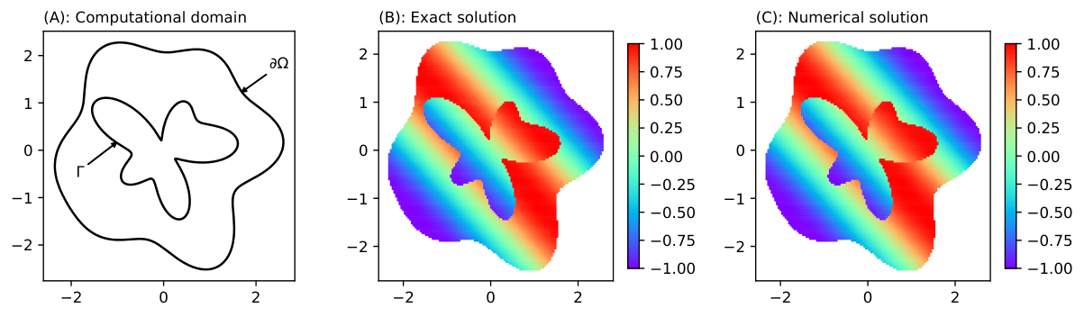
Refer to caption
Figure 9: The computational domain, exact and numerical solutions for Example 5.5. Here, the number of training data points mr=10000m_{r}=10000.
Refer to caption
Figure 10: Point-wise errors for Example 5.5. The errors of PINN, PINN-GE, and LIPR-GE are placed in the first, second, and third columns, respectively. Here, the number of training data points mr=10000m_{r}=10000.
Figure 11: The L2L^{2} and H2H^{2} convergence of the errors of Example 5.5 with respect to the number of training data points. The shaded regions are the one-standard-derivation from five runs with different training data and network initialization. Here, the number of test data points in Ω1\Omega_{1} and Ω2\Omega_{2} are N1=4044N_{1}=4044 and N2=13787N_{2}=13787, respectively.

The computational domain, the exact solution of Example (5.5), and the numerical solution obtained by LIPR-GE are shown in Fig. 9. And the point-wise L2L^{2} and H2H^{2} errors in the whole domain for PINN, PINN-GE, and LIPR-GE are presented in Fig. 10. It is observed that LIPR-GE is less accurate than Vanilla PINN and PINN-GE. One explanation is that the additional auxiliary loss terms, especially the Lipschitz regularization, make it difficult for the optimization to find the minimizer. However, our following results clearly demonstrate that LIPR-GE can still recover the exact solution up to O⁡(10−3)O(10^{-3}) accuracy in L2L^{2} and O⁡(10−2)O(10^{-2}) accuracy in H2H^{2}. Fig. 11 summarizes the convergent evolution of the L2L^{2} and H2H^{2} errors obtained by LIPR-GE with respect to the number of training data points. Clearly, the numerical results demonstrate both the L2L^{2} and H2H^{2}-convergence of the errors, which are consistent to the theoretical analysis of this paper.

6 Proofs

We present the proof of Theorem 4.1 in this section. The technique used in the following proof is similar to that used in the proof of Theorem 3 of [29]. However, our Theorem 4.1 applies to elliptic interface problems without a zero-loss assumption of interface and boundary conditions. This prevents direct use of the result from [29], which applies only to elliptic PDEs with a network solution obeying the boundary conditions exactly. Throughout this section, we assume that Assumptions 4.1 and 4.2 hold. Among the crucial technical tools used here are some Sobolev inequality and probability space filling arguments [43]. We start with the following auxiliary lemma:

Lemma 6.1.

Suppose Assumption 4.1 holds. For training data 𝒯r1mr1={𝐱r1i}i=1mr1\mathcal{T}_{r_{1}}^{m_{r_{1}}}=\{\mathbf{x}_{r_{1}}^{i}\}_{i=1}^{m_{r_{1}}}, 𝒯r2mr2={𝐱r2i}i=1mr2\mathcal{T}_{r_{2}}^{m_{r_{2}}}=\{\mathbf{x}_{r_{2}}^{i}\}_{i=1}^{m_{r_{2}}}, 𝒯bmb={𝐱bi}i=1mb\mathcal{T}_{b}^{m_{b}}=\{\mathbf{x}_{b}^{i}\}_{i=1}^{m_{b}} and 𝒯ΓmΓ={𝐱Γi}i=1mΓ\mathcal{T}_{\Gamma}^{m_{\Gamma}}=\{\mathbf{x}_{\Gamma}^{i}\}_{i=1}^{m_{\Gamma}}, if mr1m_{r_{1}}, mr2m_{r_{2}}, mbm_{b} and mΓm_{\Gamma} are large enough to satisfy that there exists 𝐱r1′∈𝒯r1\mathbf{x}_{r_{1}}^{\prime}\in\mathcal{T}_{r_{1}}, 𝐱r2′∈𝒯r2\mathbf{x}_{r_{2}}^{\prime}\in\mathcal{T}_{r_{2}}, 𝐱b′∈𝒯b\mathbf{x}_{b}^{\prime}\in\mathcal{T}_{b} and 𝐱Γ′∈𝒯Γ\mathbf{x}_{\Gamma}^{\prime}\in\mathcal{T}_{\Gamma} such that ‖𝐱r1−𝐱r1′‖2≤ϵr1\left\lVert\mathbf{x}_{r_{1}}-\mathbf{x}_{r_{1}}^{\prime}\right\rVert_{2}\leq\epsilon_{r_{1}}, ‖𝐱r2−𝐱r2′‖2≤ϵr2\left\lVert\mathbf{x}_{r_{2}}-\mathbf{x}_{r_{2}}^{\prime}\right\rVert_{2}\leq\epsilon_{r_{2}}, ‖𝐱b−𝐱b′‖2≤ϵb\left\lVert\mathbf{x}_{b}-\mathbf{x}_{b}^{\prime}\right\rVert_{2}\leq\epsilon_{b} and ‖𝐱Γ−𝐱Γ′‖2≤ϵΓ\left\lVert\mathbf{x}_{\Gamma}-\mathbf{x}_{\Gamma}^{\prime}\right\rVert_{2}\leq\epsilon_{\Gamma} for any 𝐱r1∈Ω1\mathbf{x}_{r_{1}}\in\Omega_{1}, 𝐱r2∈Ω2\mathbf{x}_{r_{2}}\in\Omega_{2}, 𝐱b∈∂Ω\mathbf{x}_{b}\in\partial\Omega and 𝐱Γ∈Γ\mathbf{x}_{\Gamma}\in\Gamma, then, we have

LossPINN​(u1,u2,𝝀)≤\displaystyle\text{Loss}^{\text{PINN}}(u_{1},u_{2};\bm{\lambda})\leq C𝒎⋅Loss𝒎PINN​(u1,u2,𝝀)+3​λr1​ϵr12​([ℒ1​[u1]]Ω12+[f1]Ω12)\displaystyle C_{\bm{m}}\cdot\text{Loss}_{\bm{m}}^{\text{PINN}}(u_{1},u_{2};\bm{\lambda})+3\lambda_{r_{1}}\epsilon_{r_{1}}^{2}\left(\big[\mathcal{L}_{1}[u_{1}]\big]_{\Omega_{1}}^{2}+\big[f_{1}\big]_{\Omega_{1}}^{2}\right)
+3​λr2​ϵr22​([ℒ2​[u2]]Ω22+[f2]Ω22)+3​λb​ϵb2​([ℬ⁡[u2]]∂Ω2+[𝒈]∂Ω2)\displaystyle+3\lambda_{r_{2}}\epsilon_{r_{2}}^{2}\left(\big[\mathcal{L}_{2}[u_{2}]\big]_{\Omega_{2}}^{2}+\big[f_{2}\big]_{\Omega_{2}}^{2}\right)+3\lambda_{b}\epsilon_{b}^{2}\left(\big[\mathcal{B}[u_{2}]\big]_{\partial\Omega}^{2}+\big[\bm{g}\big]_{\partial\Omega}^{2}\right)
+3​λΓD​ϵΓ2​([ℐD​[u1,u2]]Γ2+[𝝋]Γ2)+3​λΓN​ϵΓ2​([ℐN​[u1,u2]]Γ2+[𝝍]Γ2),\displaystyle+3\lambda_{\Gamma_{D}}\epsilon_{\Gamma}^{2}\left(\big[\mathcal{I}_{D}[u_{1},u_{2}]\big]_{\Gamma}^{2}+\big[\bm{\varphi}\big]_{\Gamma}^{2}\right)+3\lambda_{\Gamma_{N}}\epsilon_{\Gamma}^{2}\left(\big[\mathcal{I}_{N}[u_{1},u_{2}]\big]_{\Gamma}^{2}+\big[\bm{\psi}\big]_{\Gamma}^{2}\right),

where Cr1C_{r_{1}}, Cr2C_{r_{2}}, CbC_{b}, CΓC_{\Gamma} are those defined in Assumption 4.1 and

C𝒎=3​max⁡{Cr1​mr1​ϵr1d,Cr2​mr2​ϵr2d,Cb​mb​ϵbd−1,CΓ​mΓ​ϵΓd−1}.C_{\bm{m}}=3\max\{C_{r_{1}}m_{r_{1}}\epsilon_{r_{1}}^{d},C_{r_{2}}m_{r_{2}}\epsilon_{r_{2}}^{d},C_{b}m_{b}\epsilon_{b}^{d-1},C_{\Gamma}m_{\Gamma}\epsilon_{\Gamma}^{d-1}\}.
Proof.

As a consequence of Cauchy’s inequality, i.e., ‖𝐱+𝐲+𝐳‖22≤3​(‖𝐱‖22+‖𝐲‖22+‖𝐳‖22)\left\lVert\mathbf{x}+\mathbf{y}+\mathbf{z}\right\rVert_{2}^{2}\leq 3(\left\lVert\mathbf{x}\right\rVert_{2}^{2}+\left\lVert\mathbf{y}\right\rVert_{2}^{2}+\left\lVert\mathbf{z}\right\rVert_{2}^{2}) for any three vectors 𝐱,𝐲,𝐳\mathbf{x},\mathbf{y},\mathbf{z}, we deduce that for 𝐱ri,𝐱ri′∈Ωi,i=1,2\mathbf{x}_{r_{i}},\mathbf{x}_{r_{i}}^{\prime}\in\Omega_{i},i=1,2,

|ℒi​[ui]​(𝐱ri)−fi​(𝐱ri)|2≤3​(|ℒi​[ui]​(𝐱ri)−ℒi​[ui]​(𝐱ri′)|2+|ℒi​[ui]​(𝐱ri′)−fi​(𝐱ri′)|2+|fi​(𝐱ri′)−fi​(𝐱ri)|2).\displaystyle\left|\mathcal{L}_{i}[u_{i}](\mathbf{x}_{r_{i}})-f_{i}(\mathbf{x}_{r_{i}})\right|^{2}\leq 3\left(\left|\mathcal{L}_{i}[u_{i}](\mathbf{x}_{r_{i}})-\mathcal{L}_{i}[u_{i}](\mathbf{x}_{r_{i}}^{\prime})\right|^{2}+\left|\mathcal{L}_{i}[u_{i}](\mathbf{x}_{r_{i}}^{\prime})-f_{i}(\mathbf{x}_{r_{i}}^{\prime})\right|^{2}+\left|f_{i}(\mathbf{x}_{r_{i}}^{\prime})-f_{i}(\mathbf{x}_{r_{i}})\right|^{2}\right).

Similarly, for 𝐱b,𝐱b′∈∂Ω\mathbf{x}_{b},\mathbf{x}_{b}^{\prime}\in\partial\Omega, we have

‖ℬ⁡[u2]​(𝐱b)−𝒈⁡(𝐱b)‖22≤3​(‖ℬ⁡[u2]​(𝐱b)−ℬ⁡[u2]​(𝐱b′)‖22+‖ℬ⁡[u2]​(𝐱b′)−𝒈⁡(𝐱b′)‖22+‖𝒈⁡(𝐱b′)−𝒈⁡(𝐱b)‖22),\left\lVert\mathcal{B}[u_{2}](\mathbf{x}_{b})-\bm{g}(\mathbf{x}_{b})\right\rVert_{2}^{2}\leq 3\left(\left\lVert\mathcal{B}[u_{2}](\mathbf{x}_{b})-\mathcal{B}[u_{2}](\mathbf{x}_{b}^{\prime})\right\rVert_{2}^{2}+\left\lVert\mathcal{B}[u_{2}](\mathbf{x}_{b}^{\prime})-\bm{g}(\mathbf{x}_{b}^{\prime})\right\rVert_{2}^{2}+\left\lVert\bm{g}(\mathbf{x}_{b}^{\prime})-\bm{g}(\mathbf{x}_{b})\right\rVert_{2}^{2}\right),

and for 𝐱Γ,𝐱Γ′∈Γ\mathbf{x}_{\Gamma},\mathbf{x}_{\Gamma}^{\prime}\in\Gamma, we have

‖ℐD​[u1,u2]​(𝐱Γ)−𝝋⁡(𝐱Γ)‖22≤3​(CLOSE\displaystyle\left\lVert\mathcal{I}_{D}[u_{1},u_{2}](\mathbf{x}_{\Gamma})-\bm{\varphi}(\mathbf{x}_{\Gamma})\right\rVert_{2}^{2}\leq 3\big( ‖ℐD​[u1,u2]​(𝐱Γ)−ℐD​[u1,u2]​(𝐱Γ′)‖22+‖ℐD​[u1,u2]​(𝐱Γ′)−𝝋⁡(𝐱Γ′)‖22\displaystyle\left\lVert\mathcal{I}_{D}[u_{1},u_{2}](\mathbf{x}_{\Gamma})-\mathcal{I}_{D}[u_{1},u_{2}](\mathbf{x}_{\Gamma}^{\prime})\right\rVert_{2}^{2}+\left\lVert\mathcal{I}_{D}[u_{1},u_{2}](\mathbf{x}_{\Gamma}^{\prime})-\bm{\varphi}(\mathbf{x}_{\Gamma}^{\prime})\right\rVert_{2}^{2}
OPEN+‖𝝋⁡(𝐱Γ)−𝝋⁡(𝐱Γ′)‖22),\displaystyle+\left\lVert\bm{\varphi}(\mathbf{x}_{\Gamma})-\bm{\varphi}(\mathbf{x}_{\Gamma}^{\prime})\right\rVert_{2}^{2}\big),
‖ℐN​[u1,u2]​(𝐱Γ)−𝝋⁡(𝐱Γ)‖22≤3​(CLOSE\displaystyle\left\lVert\mathcal{I}_{N}[u_{1},u_{2}](\mathbf{x}_{\Gamma})-\bm{\varphi}(\mathbf{x}_{\Gamma})\right\rVert_{2}^{2}\leq 3\big( ‖ℐN​[u1,u2]​(𝐱Γ)−ℐN​[u1,u2]​(𝐱Γ′)‖22+‖ℐN​[u1,u2]​(𝐱Γ′)−𝝍⁡(𝐱Γ′)‖22\displaystyle\left\lVert\mathcal{I}_{N}[u_{1},u_{2}](\mathbf{x}_{\Gamma})-\mathcal{I}_{N}[u_{1},u_{2}](\mathbf{x}_{\Gamma}^{\prime})\right\rVert_{2}^{2}+\left\lVert\mathcal{I}_{N}[u_{1},u_{2}](\mathbf{x}_{\Gamma}^{\prime})-\bm{\psi}(\mathbf{x}_{\Gamma}^{\prime})\right\rVert_{2}^{2}
OPEN+‖𝝍⁡(𝐱Γ)−𝝍⁡(𝐱Γ′)‖22).\displaystyle+\left\lVert\bm{\psi}(\mathbf{x}_{\Gamma})-\bm{\psi}(\mathbf{x}_{\Gamma}^{\prime})\right\rVert_{2}^{2}\big).

In addition, by the conditions, for ∀𝐱r1∈Ω1\forall\mathbf{x}_{r_{1}}\in\Omega_{1}, ∀𝐱r2∈Ω2\forall\mathbf{x}_{r_{2}}\in\Omega_{2}, ∀𝐱b∈∂Ω\forall\mathbf{x}_{b}\in\partial\Omega and ∀𝐱Γ∈Γ\forall\mathbf{x}_{\Gamma}\in\Gamma, there exist 𝐱r1′∈𝒯r1mr1\mathbf{x}_{r_{1}}^{\prime}\in\mathcal{T}_{r_{1}}^{m_{r_{1}}}, 𝐱r2′∈𝒯r2mr2\mathbf{x}_{r_{2}}^{\prime}\in\mathcal{T}_{r_{2}}^{m_{r_{2}}}, 𝐱b′∈𝒯bmb\mathbf{x}_{b}^{\prime}\in\mathcal{T}_{b}^{m_{b}} and 𝐱Γ′∈𝒯ΓmΓ\mathbf{x}_{\Gamma}^{\prime}\in\mathcal{T}_{\Gamma}^{m_{\Gamma}} such that ‖𝐱r1−𝐱r1′‖2≤ϵr1\left\lVert\mathbf{x}_{r_{1}}-\mathbf{x}_{r_{1}}^{\prime}\right\rVert_{2}\leq\epsilon_{r_{1}}, ‖𝐱r2−𝐱r2′‖2≤ϵr2\left\lVert\mathbf{x}_{r_{2}}-\mathbf{x}_{r_{2}}^{\prime}\right\rVert_{2}\leq\epsilon_{r_{2}}, ‖𝐱b−𝐱b′‖2≤ϵb\left\lVert\mathbf{x}_{b}-\mathbf{x}_{b}^{\prime}\right\rVert_{2}\leq\epsilon_{b} and ‖𝐱Γ−𝐱Γ′‖2≤ϵΓ\left\lVert\mathbf{x}_{\Gamma}-\mathbf{x}_{\Gamma}^{\prime}\right\rVert_{2}\leq\epsilon_{\Gamma}. Taking

𝐋⁡(𝐱r1,𝐱r2,𝐱b,𝐱Γ,u1,u2,𝝀,𝟎)=\displaystyle\mathbf{L}(\mathbf{x}_{r_{1}},\mathbf{x}_{r_{2}},\mathbf{x}_{b},\mathbf{x}_{\Gamma};u_{1},u_{2},\bm{\lambda},\bm{0})= λr1​|ℒ1​[u1]​(𝐱r1)−f1​(𝐱r1)|2+λr2​|ℒ2​[u2]​(𝐱r2)−f2​(𝐱r2)|2\displaystyle\lambda_{r_{1}}\left|\mathcal{L}_{1}[u_{1}](\mathbf{x}_{r_{1}})-f_{1}(\mathbf{x}_{r_{1}})\right|^{2}+\lambda_{r_{2}}\left|\mathcal{L}_{2}[u_{2}](\mathbf{x}_{r_{2}})-f_{2}(\mathbf{x}_{r_{2}})\right|^{2}
+λb​‖ℬ⁡[u2]​(𝐱b)−𝒈⁡(𝐱b)‖22+λΓD​‖ℐD​[u1,u2]​(𝐱Γ)−𝝋⁡(𝐱Γ)‖22\displaystyle+\lambda_{b}\left\lVert\mathcal{B}[u_{2}](\mathbf{x}_{b})-\bm{g}(\mathbf{x}_{b})\right\rVert_{2}^{2}+\lambda_{\Gamma_{D}}\left\lVert\mathcal{I}_{D}[u_{1},u_{2}](\mathbf{x}_{\Gamma})-\bm{\varphi}(\mathbf{x}_{\Gamma})\right\rVert_{2}^{2}
+λΓN​‖ℐN​[u1,u2]​(𝐱Γ)−𝝍⁡(𝐱Γ)‖22,\displaystyle+\lambda_{\Gamma_{N}}\left\lVert\mathcal{I}_{N}[u_{1},u_{2}](\mathbf{x}_{\Gamma})-\bm{\psi}(\mathbf{x}_{\Gamma})\right\rVert_{2}^{2},

we have that

𝐋⁡(𝐱r1,𝐱r2,𝐱b,𝐱Γ,u1,u2,𝝀,𝟎)\displaystyle\mathbf{L}(\mathbf{x}_{r_{1}},\mathbf{x}_{r_{2}},\mathbf{x}_{b},\mathbf{x}_{\Gamma};u_{1},u_{2},\bm{\lambda},\bm{0})
≤\displaystyle\leq 3​𝐋​(𝐱r1′,𝐱r2′,𝐱b′,𝐱Γ′,u1,u2,𝝀,𝟎)+3​λr1​(|ℒ1​[u1]​(𝐱r1)−ℒ1​[u1]​(𝐱r1′)|2+|f1​(𝐱r1)−f1​(𝐱r1′)|2)\displaystyle 3\mathbf{L}(\mathbf{x}_{r_{1}}^{\prime},\mathbf{x}_{r_{2}}^{\prime},\mathbf{x}_{b}^{\prime},\mathbf{x}_{\Gamma}^{\prime};u_{1},u_{2},\bm{\lambda},\bm{0})+3\lambda_{r_{1}}\left(\left|\mathcal{L}_{1}[u_{1}](\mathbf{x}_{r_{1}})-\mathcal{L}_{1}[u_{1}](\mathbf{x}_{r_{1}}^{\prime})\right|^{2}+\left|f_{1}(\mathbf{x}_{r_{1}})-f_{1}(\mathbf{x}_{r_{1}}^{\prime})\right|^{2}\right)
+3​λr2​(|ℒ2​[u2]​(𝐱r2)−ℒ2​[u2]​(𝐱r2′)|2+|f2​(𝐱r2)−f2​(𝐱r2′)|2)\displaystyle+3\lambda_{r_{2}}\left(\left|\mathcal{L}_{2}[u_{2}](\mathbf{x}_{r_{2}})-\mathcal{L}_{2}[u_{2}](\mathbf{x}_{r_{2}}^{\prime})\right|^{2}+\left|f_{2}(\mathbf{x}_{r_{2}})-f_{2}(\mathbf{x}_{r_{2}}^{\prime})\right|^{2}\right)
+3​λb​(‖ℬ⁡[u2]​(𝐱b)−ℬ⁡[u2]​(𝐱b′)‖22+‖𝒈⁡(𝐱b′)−𝒈⁡(𝐱b)‖22)\displaystyle+3\lambda_{b}\left(\left\lVert\mathcal{B}[u_{2}](\mathbf{x}_{b})-\mathcal{B}[u_{2}](\mathbf{x}_{b}^{\prime})\right\rVert_{2}^{2}+\left\lVert\bm{g}(\mathbf{x}_{b}^{\prime})-\bm{g}(\mathbf{x}_{b})\right\rVert_{2}^{2}\right)
+3​λΓD​(‖ℐD​[u1,u2]​(𝐱Γ)−ℐD​[u1,u2]​(𝐱Γ′)‖22+‖𝝋⁡(𝐱Γ)−𝝋⁡(𝐱Γ′)‖22)\displaystyle+3\lambda_{\Gamma_{D}}\left(\left\lVert\mathcal{I}_{D}[u_{1},u_{2}](\mathbf{x}_{\Gamma})-\mathcal{I}_{D}[u_{1},u_{2}](\mathbf{x}_{\Gamma}^{\prime})\right\rVert_{2}^{2}+\left\lVert\bm{\varphi}(\mathbf{x}_{\Gamma})-\bm{\varphi}(\mathbf{x}_{\Gamma}^{\prime})\right\rVert_{2}^{2}\right)
+3​λΓN​(‖ℐN​[u1,u2]​(𝐱Γ)−ℐN​[u1,u2]​(𝐱Γ′)‖22+‖𝝍⁡(𝐱Γ)−𝝍⁡(𝐱Γ′)‖22)\displaystyle+3\lambda_{\Gamma_{N}}\left(\left\lVert\mathcal{I}_{N}[u_{1},u_{2}](\mathbf{x}_{\Gamma})-\mathcal{I}_{N}[u_{1},u_{2}](\mathbf{x}_{\Gamma}^{\prime})\right\rVert_{2}^{2}+\left\lVert\bm{\psi}(\mathbf{x}_{\Gamma})-\bm{\psi}(\mathbf{x}_{\Gamma}^{\prime})\right\rVert_{2}^{2}\right)
≤\displaystyle\leq 3​𝐋​(𝐱r1′,𝐱r2′,𝐱b′,𝐱Γ′,u1,u2,𝝀,𝟎)+3​λr1​ϵr12​([ℒ1​[u1]]Ω12+[f1]Ω12)+3​λr2​ϵr22​([ℒ2​[u2]]Ω22+[f2]Ω22)\displaystyle 3\mathbf{L}(\mathbf{x}_{r_{1}}^{\prime},\mathbf{x}_{r_{2}}^{\prime},\mathbf{x}_{b}^{\prime},\mathbf{x}_{\Gamma}^{\prime};u_{1},u_{2},\bm{\lambda},\bm{0})+3\lambda_{r_{1}}\epsilon_{r_{1}}^{2}\left(\big[\mathcal{L}_{1}[u_{1}]\big]_{\Omega_{1}}^{2}+\big[f_{1}\big]_{\Omega_{1}}^{2}\right)+3\lambda_{r_{2}}\epsilon_{r_{2}}^{2}\left(\big[\mathcal{L}_{2}[u_{2}]\big]_{\Omega_{2}}^{2}+\big[f_{2}\big]_{\Omega_{2}}^{2}\right)
+3​λb​ϵb2​([ℬ⁡[u2]]∂Ω2+[𝒈]∂Ω2)+3​λΓD​ϵΓ2​([ℐD​[u1,u2]]Γ2+[𝝋]Γ2)+3​λΓN​ϵΓ2​([ℐN​[u1,u2]]Γ2+[𝝍]Γ2).\displaystyle+3\lambda_{b}\epsilon_{b}^{2}\left(\big[\mathcal{B}[u_{2}]\big]_{\partial\Omega}^{2}+\big[\bm{g}\big]_{\partial\Omega}^{2}\right)+3\lambda_{\Gamma_{D}}\epsilon_{\Gamma}^{2}\left(\big[\mathcal{I}_{D}[u_{1},u_{2}]\big]_{\Gamma}^{2}+\big[\bm{\varphi}\big]_{\Gamma}^{2}\right)+3\lambda_{\Gamma_{N}}\epsilon_{\Gamma}^{2}\left(\big[\mathcal{I}_{N}[u_{1},u_{2}]\big]_{\Gamma}^{2}+\big[\bm{\psi}\big]_{\Gamma}^{2}\right).

For 𝐱r1i∈𝒯r1mr1\mathbf{x}_{r_{1}}^{i}\in\mathcal{T}_{r_{1}}^{m_{r_{1}}}, 𝐱r2i∈𝒯r2mr2\mathbf{x}_{r_{2}}^{i}\in\mathcal{T}_{r_{2}}^{m_{r_{2}}}, 𝐱bi∈𝒯bmb\mathbf{x}^{i}_{b}\in\mathcal{T}_{b}^{m_{b}} and 𝐱Γi∈𝒯ΓmΓ\mathbf{x}^{i}_{\Gamma}\in\mathcal{T}_{\Gamma}^{m_{\Gamma}}, we denote the Voronoi cell associated with 𝐱r1i\mathbf{x}_{r_{1}}^{i}, 𝐱r2i\mathbf{x}_{r_{2}}^{i}, 𝐱bi\mathbf{x}_{b}^{i}, 𝐱Γi\mathbf{x}_{\Gamma}^{i} as A𝐱r1iA_{\mathbf{x}_{r_{1}}^{i}}, A𝐱r2iA_{\mathbf{x}_{r_{2}}^{i}}, A𝐱biA_{\mathbf{x}_{b}^{i}} and A𝐱ΓiA_{\mathbf{x}_{\Gamma}^{i}} , respectively, i.e.,

A𝐱r1i={𝐱∈Ω1|‖𝐱−𝐱r1i‖2=min𝐱′∈𝒯r1mr1‖𝐱−𝐱′‖2},A𝐱r2i={x∈Ω2|‖𝐱−𝐱r2i‖2=min𝐱′∈𝒯r2mr2‖𝐱−𝐱′‖2},\displaystyle A_{\mathbf{x}_{r_{1}}^{i}}=\{\mathbf{x}\in\Omega_{1}\ \big|\ \left\lVert\mathbf{x}-\mathbf{x}_{r_{1}}^{i}\right\rVert_{2}=\min_{\mathbf{x}^{\prime}\in\mathcal{T}_{r_{1}}^{m_{r_{1}}}}\left\lVert\mathbf{x}-\mathbf{x}^{\prime}\right\rVert_{2}\},\quad A_{\mathbf{x}_{r_{2}}^{i}}=\{x\in\Omega_{2}\ \big|\ \left\lVert\mathbf{x}-\mathbf{x}_{r_{2}}^{i}\right\rVert_{2}=\min_{\mathbf{x}^{\prime}\in\mathcal{T}_{r_{2}}^{m_{r_{2}}}}\left\lVert\mathbf{x}-\mathbf{x}^{\prime}\right\rVert_{2}\},
A𝐱bi={𝐱∈∂Ω|‖x−𝐱ib‖2=minx′∈𝒯bmb‖𝐱−𝐱′‖2},A𝐱Γi={𝐱∈Γ|‖𝐱−𝐱iΓ‖2=minx′∈𝒯ΓmΓ‖𝐱−𝐱′‖2},\displaystyle A_{\mathbf{x}^{i}_{b}}=\{\mathbf{x}\in\partial\Omega\ \big|\ \left\lVert x-\mathbf{x}^{i}_{b}\right\rVert_{2}=\min_{x^{\prime}\in\mathcal{T}_{b}^{m_{b}}}\left\lVert\mathbf{x}-\mathbf{x}^{\prime}\right\rVert_{2}\},\quad A_{\mathbf{x}^{i}_{\Gamma}}=\{\mathbf{x}\in\Gamma\ \big|\ \left\lVert\mathbf{x}-\mathbf{x}^{i}_{\Gamma}\right\rVert_{2}=\min_{x^{\prime}\in\mathcal{T}_{\Gamma}^{m_{\Gamma}}}\left\lVert\mathbf{x}-\mathbf{x}^{\prime}\right\rVert_{2}\},

and let ωr1i=μr1​(A𝐱r1i)\omega^{i}_{r_{1}}=\mu_{r_{1}}(A_{\mathbf{x}^{i}_{r_{1}}}) , ωr2i=μr2​(A𝐱r2i)\omega^{i}_{r_{2}}=\mu_{r_{2}}(A_{\mathbf{x}^{i}_{r_{2}}}), ωbi=μb​(A𝐱bi)\omega^{i}_{b}=\mu_{b}(A_{\mathbf{x}^{i}_{b}}) and ωΓi=μΓ​(A𝐱Γi)\omega^{i}_{\Gamma}=\mu_{\Gamma}(A_{\mathbf{x}^{i}_{\Gamma}}). By taking the expectation with respect to (𝐱r1,𝐱r2,𝐱b,𝐱Γ)∼μ=μr1×μr2×μb×μΓ(\mathbf{x}_{r_{1}},\mathbf{x}_{r_{2}},\mathbf{x}_{b},\mathbf{x}_{\Gamma})\sim\mu=\mu_{r_{1}}\times\mu_{r_{2}}\times\mu_{b}\times\mu_{\Gamma}, we obtain that

𝔼μ​[𝐋⁡(𝐱r1,𝐱r2,𝐱b,𝐱Γ,u1,u2,𝝀,𝟎)]\displaystyle\mathbb{E}_{\mu}[\mathbf{L}(\mathbf{x}_{r_{1}},\mathbf{x}_{r_{2}},\mathbf{x}_{b},\mathbf{x}_{\Gamma};u_{1},u_{2},\bm{\lambda},\bm{0})]
=\displaystyle= ∑i=1mΓ∑j=1mb∑k=1mr1∑l=1mr2∫A𝐱Γi∫A𝐱bj∫A𝐱r1k∫A𝐱r2l𝐋⁡(𝐱r1,𝐱r2,𝐱b,𝐱Γ,u1,u2,𝝀,𝟎)​𝑑μ\displaystyle\sum_{i=1}^{m_{\Gamma}}\sum_{j=1}^{m_{b}}\sum_{k=1}^{m_{r_{1}}}\sum_{l=1}^{m_{r_{2}}}\int_{A_{\mathbf{x}_{\Gamma}^{i}}}\int_{A_{\mathbf{x}_{b}^{j}}}\int_{A_{\mathbf{x}_{r_{1}}^{k}}}\int_{A_{\mathbf{x}_{r_{2}}^{l}}}\mathbf{L}(\mathbf{x}_{r_{1}},\mathbf{x}_{r_{2}},\mathbf{x}_{b},\mathbf{x}_{\Gamma};u_{1},u_{2},\bm{\lambda},\bm{0})d\mu
≤\displaystyle\leq 3​∑i=1mΓ∑j=1mb∑k=1mr1∑l=1mr2ωΓi​ωbj​ωr1k​ωr2l​𝐋​(𝐱r1k,𝐱r2l,𝐱bj,𝐱Γi,u1,u2,𝝀,𝟎)+3​λr1​ϵr12​([ℒ1​[u1]]Ω12+[f1]Ω12)\displaystyle 3\sum_{i=1}^{m_{\Gamma}}\sum_{j=1}^{m_{b}}\sum_{k=1}^{m_{r_{1}}}\sum_{l=1}^{m_{r_{2}}}\omega_{\Gamma}^{i}\omega_{b}^{j}\omega_{r_{1}}^{k}\omega_{r_{2}}^{l}\mathbf{L}(\mathbf{x}_{r_{1}}^{k},\mathbf{x}_{r_{2}}^{l},\mathbf{x}_{b}^{j},\mathbf{x}_{\Gamma}^{i};u_{1},u_{2},\bm{\lambda},\bm{0})+3\lambda_{r_{1}}\epsilon_{r_{1}}^{2}\left(\big[\mathcal{L}_{1}[u_{1}]\big]_{\Omega_{1}}^{2}+\big[f_{1}\big]_{\Omega_{1}}^{2}\right)
+3​λr2​ϵr22​([ℒ2​[u2]]Ω22+[f2]Ω22)+3​λb​ϵb2​([ℬ⁡[u2]]∂Ω2+[𝒈]∂Ω2)\displaystyle+3\lambda_{r_{2}}\epsilon_{r_{2}}^{2}\left(\big[\mathcal{L}_{2}[u_{2}]\big]_{\Omega_{2}}^{2}+\big[f_{2}\big]_{\Omega_{2}}^{2}\right)+3\lambda_{b}\epsilon_{b}^{2}\left(\big[\mathcal{B}[u_{2}]\big]_{\partial\Omega}^{2}+\big[\bm{g}\big]_{\partial\Omega}^{2}\right)
+3​λΓD​ϵΓ2​([ℐD​[u1,u2]]Γ2+[𝝋]Γ2)+3​λΓN​ϵΓ2​([ℐN​[u1,u2]]Γ2+[𝝍]Γ2),\displaystyle+3\lambda_{\Gamma_{D}}\epsilon_{\Gamma}^{2}\left(\big[\mathcal{I}_{D}[u_{1},u_{2}]\big]_{\Gamma}^{2}+\big[\bm{\varphi}\big]_{\Gamma}^{2}\right)+3\lambda_{\Gamma_{N}}\epsilon_{\Gamma}^{2}\left(\big[\mathcal{I}_{N}[u_{1},u_{2}]\big]_{\Gamma}^{2}+\big[\bm{\psi}\big]_{\Gamma}^{2}\right),

where we have used the fact that ∑i=1mr1ωr1i=1\sum_{i=1}^{m_{r_{1}}}\omega^{i}_{r_{1}}=1, ∑i=1mr2ωr2i=1\sum_{i=1}^{m_{r_{2}}}\omega^{i}_{r_{2}}=1, ∑i=1mbωbi=1\sum_{i=1}^{m_{b}}\omega^{i}_{b}=1 and ∑i=1mΓωΓi=1\sum_{i=1}^{m_{\Gamma}}\omega^{i}_{\Gamma}=1.

Next, we give the estimation of the first term on the right. Taking ωr1mr1,∗=maxi⁡ωr1i\omega_{r_{1}}^{m_{r_{1}},*}=\max_{i}\omega_{r_{1}}^{i}, ωr2mr2,∗=maxi⁡ωr2i\omega_{r_{2}}^{m_{r_{2}},*}=\max_{i}\omega_{r_{2}}^{i}, ωbmb,∗=maxi⁡ωbi\omega_{b}^{m_{b},*}=\max_{i}\omega^{i}_{b} and ωΓmΓ,∗=maxi⁡ωΓi\omega_{\Gamma}^{m_{\Gamma},*}=\max_{i}\omega^{i}_{\Gamma}, yields that

3​∑i=1mΓ∑j=1mb∑k=1mr1∑l=1mr2ωΓi​ωbj​ωr1k​ωr2l​𝐋​(𝐱r1k,𝐱r2l,𝐱bj,𝐱Γi,u1,u2,𝝀,𝟎)\displaystyle 3\sum_{i=1}^{m_{\Gamma}}\sum_{j=1}^{m_{b}}\sum_{k=1}^{m_{r_{1}}}\sum_{l=1}^{m_{r_{2}}}\omega_{\Gamma}^{i}\omega_{b}^{j}\omega_{r_{1}}^{k}\omega_{r_{2}}^{l}\mathbf{L}(\mathbf{x}_{r_{1}}^{k},\mathbf{x}_{r_{2}}^{l},\mathbf{x}_{b}^{j},\mathbf{x}_{\Gamma}^{i};u_{1},u_{2},\bm{\lambda},\bm{0}) (8)
≤\displaystyle\leq 3mr1ωr1mr1,∗⋅λr1mr1∑i=1mr1|ℒ1[u1](𝐱r1i)−f1(𝐱r1i)|2+3mr2ωr2mr2,∗⋅λr2mr2∑i=1mr2|ℒ2[u2](𝐱r2i)−f2(𝐱r2i)|2\displaystyle 3m_{r_{1}}\omega_{r_{1}}^{m_{r_{1}},*}\cdot\frac{\lambda_{r_{1}}}{m_{r_{1}}}\sum_{i=1}^{m_{r_{1}}}\left|\mathcal{L}_{1}[u_{1}](\mathbf{x}_{r_{1}}^{i})-f_{1}(\mathbf{x}_{r_{1}}^{i})\right|^{2}+3m_{r_{2}}\omega_{r_{2}}^{m_{r_{2}},*}\cdot\frac{\lambda_{r_{2}}}{m_{r_{2}}}\sum_{i=1}^{m_{r_{2}}}\left|\mathcal{L}_{2}[u_{2}](\mathbf{x}_{r_{2}}^{i})-f_{2}(\mathbf{x}_{r_{2}}^{i})\right|^{2}
+3mΓωΓmΓ,∗⋅(λΓDmΓ∑i=1mΓ‖ℐD[u1,u2](𝐱Γi)−𝝋(𝐱Γi)‖22+λΓNmΓ∑i=1mΓ‖ℐN[u1,u2](𝐱Γi)−𝝍(𝐱Γi)‖22)\displaystyle+3m_{\Gamma}\omega_{\Gamma}^{m_{\Gamma},*}\cdot\left(\frac{\lambda_{\Gamma_{D}}}{m_{\Gamma}}\sum_{i=1}^{m_{\Gamma}}\left\lVert\mathcal{I}_{D}[u_{1},u_{2}](\mathbf{x}_{\Gamma}^{i})-\bm{\varphi}(\mathbf{x}_{\Gamma}^{i})\right\rVert_{2}^{2}+\frac{\lambda_{\Gamma_{N}}}{m_{\Gamma}}\sum_{i=1}^{m_{\Gamma}}\left\lVert\mathcal{I}_{N}[u_{1},u_{2}](\mathbf{x}_{\Gamma}^{i})-\bm{\psi}(\mathbf{x}_{\Gamma}^{i})\right\rVert_{2}^{2}\right)
+3mbωbmb,∗⋅λbmb∑i=1mb‖ℬ[u2](𝐱bi)−𝒈(𝐱bi)‖22,\displaystyle+3m_{b}\omega_{b}^{m_{b},*}\cdot\frac{\lambda_{b}}{m_{b}}\sum_{i=1}^{m_{b}}\left\lVert\mathcal{B}[u_{2}](\mathbf{x}_{b}^{i})-\bm{g}(\mathbf{x}_{b}^{i})\right\rVert_{2}^{2},

where we have used the fact that mr1​ωr1mr1,∗,mr2​ωr2mr2,∗,mb​ωbmb,∗,mΓ​ωΓmΓ,∗≥1m_{r_{1}}\omega_{r_{1}}^{m_{r_{1}},*},m_{r_{2}}\omega_{r_{2}}^{m_{r_{2}},*},m_{b}\omega_{b}^{m_{b},*},m_{\Gamma}\omega_{\Gamma}^{m_{\Gamma},*}\geq 1.

Let Bϵ​(𝐱)B_{\epsilon}(\mathbf{x}) be a closed ball centered at 𝐱\mathbf{x} with radius ϵ\epsilon. Let Pr1∗=max𝐱∈Ω1⁡μr1​(Bϵr1​(𝐱)∩Ω1)P_{r_{1}}^{*}=\max_{\mathbf{x}\in\Omega_{1}}\mu_{r_{1}}(B_{\epsilon_{r_{1}}}(\mathbf{x})\cap\Omega_{1}), Pr2∗=max𝐱∈Ω2⁡μr2​(Bϵr2​(𝐱)∩Ω2)P_{r_{2}}^{*}=\max_{\mathbf{x}\in\Omega_{2}}\mu_{r_{2}}(B_{\epsilon_{r_{2}}}(\mathbf{x})\cap\Omega_{2}), Pb∗=max𝐱∈∂Ω⁡μb​(Bϵb​(𝐱)∩∂Ω)P_{b}^{*}=\max_{\mathbf{x}\in\partial\Omega}\mu_{b}(B_{\epsilon_{b}}(\mathbf{x})\cap\partial\Omega) and PΓ∗=max𝐱∈Γ⁡μΓ​(BϵΓ​(𝐱)∩Γ)P_{\Gamma}^{*}=\max_{\mathbf{x}\in\Gamma}\mu_{\Gamma}(B_{\epsilon_{\Gamma}}(\mathbf{x})\cap\Gamma). Then for any 𝐱r1∈Ω1\mathbf{x}_{r_{1}}\in\Omega_{1}, 𝐱r2∈Ω2\mathbf{x}_{r_{2}}\in\Omega_{2}, 𝐱b∈∂Ω\mathbf{x}_{b}\in\partial\Omega and 𝐱Γ∈Γ\mathbf{x}_{\Gamma}\in\Gamma, there exists 𝐱r1′∈𝒯r1\mathbf{x}_{r_{1}}^{\prime}\in\mathcal{T}_{r_{1}}, 𝐱r2′∈𝒯r2\mathbf{x}_{r_{2}}^{\prime}\in\mathcal{T}_{r_{2}}, 𝐱b′∈𝒯b\mathbf{x}_{b}^{\prime}\in\mathcal{T}_{b} and 𝐱Γ′∈𝒯Γ\mathbf{x}_{\Gamma}^{\prime}\in\mathcal{T}_{\Gamma} such that ‖𝐱r1−𝐱r1′‖2≤ϵr1\left\lVert\mathbf{x}_{r_{1}}-\mathbf{x}_{r_{1}}^{\prime}\right\rVert_{2}\leq\epsilon_{r_{1}}, ‖𝐱r2−𝐱r2′‖2≤ϵr2\left\lVert\mathbf{x}_{r_{2}}-\mathbf{x}_{r_{2}}^{\prime}\right\rVert_{2}\leq\epsilon_{r_{2}}, ‖𝐱b−𝐱b′‖2≤ϵb\left\lVert\mathbf{x}_{b}-\mathbf{x}_{b}^{\prime}\right\rVert_{2}\leq\epsilon_{b} and ‖𝐱Γ−𝐱Γ′‖2≤ϵΓ\left\lVert\mathbf{x}_{\Gamma}-\mathbf{x}_{\Gamma}^{\prime}\right\rVert_{2}\leq\epsilon_{\Gamma} for each ii, there are closed balls Bϵr1B_{\epsilon_{r_{1}}}, Bϵr2B_{\epsilon_{r_{2}}}, BϵbB_{\epsilon_{b}} and BϵΓB_{\epsilon_{\Gamma}} that include A𝐱r1iA_{\mathbf{x}_{r_{1}}^{i}}, A𝐱r2iA_{\mathbf{x}_{r_{2}}^{i}}, A𝐱biA_{\mathbf{x}_{b}^{i}} and A𝐱ΓiA_{\mathbf{x}_{\Gamma}^{i}}, respectively. These facts, together with Assumption 4.1 imply that

ωr1mr1,∗≤Pr1∗≤Cr1​ϵr1d,ωr2mr2,∗≤Pr2∗≤Cr2​ϵr2d,ωbmb,∗≤Pb∗≤Cb​ϵbd−1,ωΓmΓ,∗≤PΓ∗≤CΓ​ϵΓd−1.\omega_{r_{1}}^{m_{r_{1}},*}\leq P_{r_{1}}^{*}\leq C_{r_{1}}\epsilon_{r_{1}}^{d},\ \omega_{r_{2}}^{m_{r_{2}},*}\leq P_{r_{2}}^{*}\leq C_{r_{2}}\epsilon_{r_{2}}^{d},\ \omega_{b}^{m_{b},*}\leq P_{b}^{*}\leq C_{b}\epsilon_{b}^{d-1},\ \omega_{\Gamma}^{m_{\Gamma},*}\leq P_{\Gamma}^{*}\leq C_{\Gamma}\epsilon_{\Gamma}^{d-1}. (9)

With the estimations (8) and (9), we obtain that

𝔼μ​[𝐋⁡(𝐱r1,𝐱r2,𝐱b,𝐱Γ,u1,u2,𝝀,𝟎)]\displaystyle\mathbb{E}_{\mu}[\mathbf{L}(\mathbf{x}_{r_{1}},\mathbf{x}_{r_{2}},\mathbf{x}_{b},\mathbf{x}_{\Gamma};u_{1},u_{2},\bm{\lambda},\bm{0})]
≤\displaystyle\leq 3Cr1mr1ϵr1d⋅λr1mr1∑i=1mr1|ℒ1[u1](𝐱r1i)−f1(𝐱r1i)|2+3Cr2mr2ϵr2d⋅λr2mr2∑i=1mr2|ℒ2[u2](𝐱r2i)−f2(𝐱r2i)|2\displaystyle 3C_{r_{1}}m_{r_{1}}\epsilon_{r_{1}}^{d}\cdot\frac{\lambda_{r_{1}}}{m_{r_{1}}}\sum_{i=1}^{m_{r_{1}}}\left|\mathcal{L}_{1}[u_{1}](\mathbf{x}_{r_{1}}^{i})-f_{1}(\mathbf{x}_{r_{1}}^{i})\right|^{2}+3C_{r_{2}}m_{r_{2}}\epsilon_{r_{2}}^{d}\cdot\frac{\lambda_{r_{2}}}{m_{r_{2}}}\sum_{i=1}^{m_{r_{2}}}\left|\mathcal{L}_{2}[u_{2}](\mathbf{x}_{r_{2}}^{i})-f_{2}(\mathbf{x}_{r_{2}}^{i})\right|^{2}
+3CΓmΓϵΓd−1⋅(λΓDmΓ∑i=1mΓ‖ℐD[u1,u2](𝐱Γi)−𝝋(𝐱Γi)‖22+λΓNmΓ∑i=1mΓ‖ℐN[u1,u2](𝐱Γi)−𝝍(𝐱Γi)‖22)\displaystyle+3C_{\Gamma}m_{\Gamma}\epsilon_{\Gamma}^{d-1}\cdot\left(\frac{\lambda_{\Gamma_{D}}}{m_{\Gamma}}\sum_{i=1}^{m_{\Gamma}}\left\lVert\mathcal{I}_{D}[u_{1},u_{2}](\mathbf{x}_{\Gamma}^{i})-\bm{\varphi}(\mathbf{x}_{\Gamma}^{i})\right\rVert_{2}^{2}+\frac{\lambda_{\Gamma_{N}}}{m_{\Gamma}}\sum_{i=1}^{m_{\Gamma}}\left\lVert\mathcal{I}_{N}[u_{1},u_{2}](\mathbf{x}_{\Gamma}^{i})-\bm{\psi}(\mathbf{x}_{\Gamma}^{i})\right\rVert_{2}^{2}\right)
+3Cbmbϵbd−1⋅λbmb∑j=1mb‖ℬ[u2](𝐱bj)−𝒈(𝐱bj)‖22+3λr1ϵr12([ℒ1[u1]]Ω12+[f1]Ω12)\displaystyle+3C_{b}m_{b}\epsilon_{b}^{d-1}\cdot\frac{\lambda_{b}}{m_{b}}\sum_{j=1}^{m_{b}}\left\lVert\mathcal{B}[u_{2}](\mathbf{x}_{b}^{j})-\bm{g}(\mathbf{x}_{b}^{j})\right\rVert_{2}^{2}+3\lambda_{r_{1}}\epsilon_{r_{1}}^{2}\left(\big[\mathcal{L}_{1}[u_{1}]\big]_{\Omega_{1}}^{2}+\big[f_{1}\big]_{\Omega_{1}}^{2}\right)
+3​λr2​ϵr22​([ℒ2​[u2]]Ω22+[f2]Ω22)+3​λb​ϵb2​([ℬ⁡[u2]]∂Ω2+[𝒈]∂Ω2)\displaystyle+3\lambda_{r_{2}}\epsilon_{r_{2}}^{2}\left(\big[\mathcal{L}_{2}[u_{2}]\big]_{\Omega_{2}}^{2}+\big[f_{2}\big]_{\Omega_{2}}^{2}\right)+3\lambda_{b}\epsilon_{b}^{2}\left(\big[\mathcal{B}[u_{2}]\big]_{\partial\Omega}^{2}+\big[\bm{g}\big]_{\partial\Omega}^{2}\right)
+3​λΓD​ϵΓ2​([ℐD​[u1,u2]]Γ2+[𝝋]Γ2)+3​λΓN​ϵΓ2​([ℐN​[u1,u2]]Γ2+[𝝍]Γ2).\displaystyle+3\lambda_{\Gamma_{D}}\epsilon_{\Gamma}^{2}\left(\big[\mathcal{I}_{D}[u_{1},u_{2}]\big]_{\Gamma}^{2}+\big[\bm{\varphi}\big]_{\Gamma}^{2}\right)+3\lambda_{\Gamma_{N}}\epsilon_{\Gamma}^{2}\left(\big[\mathcal{I}_{N}[u_{1},u_{2}]\big]_{\Gamma}^{2}+\big[\bm{\psi}\big]_{\Gamma}^{2}\right).

Finally, we conclude the proof by taking C𝒎=3​max⁡{Cr1​mr1​ϵr1d,Cr2​mr2​ϵr2d,Cb​mb​ϵbd−1,CΓ​mΓ​ϵΓd−1}C_{\bm{m}}=3\max\{C_{r_{1}}m_{r_{1}}\epsilon_{r_{1}}^{d},C_{r_{2}}m_{r_{2}}\epsilon_{r_{2}}^{d},C_{b}m_{b}\epsilon_{b}^{d-1},C_{\Gamma}m_{\Gamma}\epsilon_{\Gamma}^{d-1}\}. ∎

With Lemma 6.1 and Assumption 4.1, we are able to quantify the generalization error and provide an upper bound of the expected unregularized PINN loss (7).

Lemma 6.2.

Suppose Assumption 4.1 holds. Suppose that u1,u2u_{1},u_{2} satisfy

Rr1​(u1)<∞,Rr2​(u2)<∞,Rb​(u2)<∞,RΓD​(u1,u2)<∞,RΓN​(u1,u2)<∞,R_{r_{1}}(u_{1})<\infty,\ R_{r_{2}}(u_{2})<\infty,\ R_{b}(u_{2})<\infty,\ R_{\Gamma_{D}}(u_{1},u_{2})<\infty,\ R_{\Gamma_{N}}(u_{1},u_{2})<\infty,

and f1,f2,𝛙,𝛗,𝐠f_{1},f_{2},\bm{\psi},\bm{\varphi},\bm{g} satisfy

[f1]Ω1,[f2]Ω2,[𝒈]∂Ω,[𝝋]Γ,[𝝍]Γ<∞.\big[f_{1}\big]_{\Omega_{1}},\ \big[f_{2}\big]_{\Omega_{2}},\ \big[\bm{g}\big]_{\partial\Omega},\ \big[\bm{\varphi}\big]_{\Gamma},\ \big[\bm{\psi}\big]_{\Gamma}<\infty.

Let mr1m_{r_{1}}, mr2m_{r_{2}}, mbm_{b} and mΓm_{\Gamma} be the number of iid samples from μr1\mu_{r_{1}}, μr2\mu_{r_{2}}, μb\mu_{b} and μΓ\mu_{\Gamma}, respectively. Let 𝛌=(λr1,λr2,λb,λΓD,λΓN)\bm{\lambda}=(\lambda_{r_{1}},\lambda_{r_{2}},\lambda_{b},\lambda_{\Gamma_{D}},\lambda_{\Gamma_{N}}) be a fixed vector. Then, with probability at least,

P=P⁡(mr1)​P​(mr2)​P​(mb)​P​(mΓ),where ​P​(m)=(1−m​(1−1/m)m),P=P(m_{r_{1}})P(m_{r_{2}})P(m_{b})P(m_{\Gamma}),\quad\text{where }P(m)=(1-\sqrt{m}(1-1/\sqrt{m})^{m}),

we have

LossPINN​(u1,u2,𝝀)≤C𝒎⋅Loss𝒎​(u1,u2,𝝀,𝝀^𝒎R)+C′​(mr1−1d+mr2−1d+mb−1d−1+mΓ−1d−1).\text{Loss}^{\text{PINN}}(u_{1},u_{2};\bm{\lambda})\leq C_{\bm{m}}\cdot\text{Loss}_{\bm{m}}(u_{1},u_{2};\bm{\lambda},\bm{\hat{\lambda}}_{\bm{m}}^{R})+C^{\prime}(m_{r_{1}}^{-\frac{1}{d}}+m_{r_{2}}^{-\frac{1}{d}}+m_{b}^{-\frac{1}{d-1}}+m_{\Gamma}^{-\frac{1}{d-1}}).

Here, 𝛌^𝐦R=(λ^r1,𝐦R,λ^r2,𝐦R,λ^b,𝐦R,λ^ΓD,𝐦R,λ^ΓN,𝐦R)\bm{\hat{\lambda}}_{\bm{m}}^{R}=(\hat{\lambda}_{r_{1},\bm{m}}^{R},\hat{\lambda}_{r_{2},\bm{m}}^{R},\hat{\lambda}_{b,\bm{m}}^{R},\hat{\lambda}_{\Gamma_{D},\bm{m}}^{R},\hat{\lambda}_{\Gamma_{N},\bm{m}}^{R}). Specifically,

λ^r1,𝒎R=3​λr1​d​cr1−2dC𝒎⋅mr1−1d,λ^r2,𝒎R=3​λr2​d​cr2−2dC𝒎⋅mr2−1d,λ^b,𝒎R=3​λb​d​cb−2d−1C𝒎⋅mb−1d−1,\displaystyle\hat{\lambda}_{r_{1},\bm{m}}^{R}=\frac{3\lambda_{r_{1}}dc_{r_{1}}^{-\frac{2}{d}}}{C_{\bm{m}}}\cdot m_{r_{1}}^{-\frac{1}{d}},\quad\hat{\lambda}_{r_{2},\bm{m}}^{R}=\frac{3\lambda_{r_{2}}dc_{r_{2}}^{-\frac{2}{d}}}{C_{\bm{m}}}\cdot m_{r_{2}}^{-\frac{1}{d}},\quad\hat{\lambda}_{b,\bm{m}}^{R}=\frac{3\lambda_{b}dc_{b}^{-\frac{2}{d-1}}}{C_{\bm{m}}}\cdot m_{b}^{-\frac{1}{d-1}},
λ^ΓD,𝒎R=3​λΓD​d​cΓ−2d−1C𝒎⋅mΓ−1d−1,λ^ΓN,𝒎R=3​λΓN​d​cΓ−2d−1C𝒎⋅mΓ−1d−1.\displaystyle\hat{\lambda}_{\Gamma_{D},\bm{m}}^{R}=\frac{3\lambda_{\Gamma_{D}}dc_{\Gamma}^{-\frac{2}{d-1}}}{C_{\bm{m}}}\cdot m_{\Gamma}^{-\frac{1}{d-1}},\quad\hat{\lambda}_{\Gamma_{N},\bm{m}}^{R}=\frac{3\lambda_{\Gamma_{N}}dc_{\Gamma}^{-\frac{2}{d-1}}}{C_{\bm{m}}}\cdot m_{\Gamma}^{-\frac{1}{d-1}}.

C𝒎=3​max⁡{κr1​dd​mr112,κr2​dd​mr212,κb​dd−1​mb12,κΓ​dd−1​mΓ12}C_{\bm{m}}=3\max\{\kappa_{r_{1}}\sqrt{d}^{d}m_{r_{1}}^{\frac{1}{2}},\kappa_{r_{2}}\sqrt{d}^{d}m_{r_{2}}^{\frac{1}{2}},\kappa_{b}\sqrt{d}^{d-1}m_{b}^{\frac{1}{2}},\kappa_{\Gamma}\sqrt{d}^{d-1}m_{\Gamma}^{\frac{1}{2}}\} where κr1=Cr1cr1\kappa_{r_{1}}=\frac{C_{r_{1}}}{c_{r_{1}}}, κr2=Cr2cr2\kappa_{r_{2}}=\frac{C_{r_{2}}}{c_{r_{2}}}, κb=Cbcb\kappa_{b}=\frac{C_{b}}{c_{b}}, κΓ=CΓcΓ\kappa_{\Gamma}=\frac{C_{\Gamma}}{c_{\Gamma}}. And C′C^{\prime} is a constant that depends only on 𝛌\bm{\lambda}, dd, cr1c_{r_{1}}, cr2c_{r_{2}}, cbc_{b}, cΓc_{\Gamma}, f1f_{1}, f2f_{2}, 𝐠\bm{g}, 𝛗\bm{\varphi}, 𝛙\bm{\psi}.

Proof.

Since 𝒯r1={𝐱r1i}i=1mr1\mathcal{T}_{r_{1}}=\{\mathbf{x}_{r_{1}}^{i}\}_{i=1}^{m_{r_{1}}} be iid samples from μr1\mu_{r_{1}} on Ω1\Omega_{1}, 𝒯r2={𝐱r2i}i=1mr2\mathcal{T}_{r_{2}}=\{\mathbf{x}_{r_{2}}^{i}\}_{i=1}^{m_{r_{2}}} be iid samples from μr2\mu_{r_{2}} on Ω2\Omega_{2}, 𝒯b={𝐱bi}i=1mb\mathcal{T}_{b}=\{\mathbf{x}_{b}^{i}\}_{i=1}^{m_{b}} be iid samples from μb\mu_{b} on ∂Ω\partial\Omega and 𝒯Γ={𝐱Γi}i=1mΓ\mathcal{T}_{\Gamma}=\{\mathbf{x}_{\Gamma}^{i}\}_{i=1}^{m_{\Gamma}} be iid samples from μΓ\mu_{\Gamma} on Γ\Gamma, respectively, therefore, by Lemma B.2 in [29], with probability at least

P=P⁡(mr1)​P​(mr2)​P​(mb)​P​(mΓ),where ​P​(m)=(1−m​(1−1/m)m),P=P(m_{r_{1}})P(m_{r_{2}})P(m_{b})P(m_{\Gamma}),\quad\text{where }P(m)=(1-\sqrt{m}(1-1/\sqrt{m})^{m}), (10)

for ∀𝐱r1∈Ω1\forall\mathbf{x}_{r_{1}}\in\Omega_{1}, ∀𝐱r2∈Ω2\forall\mathbf{x}_{r_{2}}\in\Omega_{2}, ∀𝐱b∈∂Ω\forall\mathbf{x}_{b}\in\partial\Omega and ∀𝐱Γ∈Γ\forall\mathbf{x}_{\Gamma}\in\Gamma, there exists 𝐱r1′∈𝒯r1mr1\mathbf{x}_{r_{1}}^{\prime}\in\mathcal{T}_{r_{1}}^{m_{r_{1}}}, 𝐱r2′∈𝒯r2mr2\mathbf{x}_{r_{2}}^{\prime}\in\mathcal{T}_{r_{2}}^{m_{r_{2}}}, 𝐱b′∈𝒯bmb\mathbf{x}_{b}^{\prime}\in\mathcal{T}_{b}^{m_{b}} and 𝐱Γ′∈𝒯ΓmΓ\mathbf{x}_{\Gamma}^{\prime}\in\mathcal{T}_{\Gamma}^{m_{\Gamma}} such that ‖𝐱r1−𝐱r1′‖2≤d​cr1−1d​mr1−12​d\left\lVert\mathbf{x}_{r_{1}}-\mathbf{x}_{r_{1}}^{\prime}\right\rVert_{2}\leq\sqrt{d}c_{r_{1}}^{-\frac{1}{d}}m_{r_{1}}^{-\frac{1}{2d}}, ‖𝐱r2−𝐱r2′‖2≤d​cr2−1d​mr2−12​d\left\lVert\mathbf{x}_{r_{2}}-\mathbf{x}_{r_{2}}^{\prime}\right\rVert_{2}\leq\sqrt{d}c_{r_{2}}^{-\frac{1}{d}}m_{r_{2}}^{-\frac{1}{2d}}, ‖𝐱b−𝐱b′‖2≤d​cb−1d−1​mb−12​(d−1)\left\lVert\mathbf{x}_{b}-\mathbf{x}_{b}^{\prime}\right\rVert_{2}\leq\sqrt{d}c^{-\frac{1}{d-1}}_{b}m_{b}^{-\frac{1}{2(d-1)}} and ‖𝐱Γ−𝐱Γ′‖2≤d​cΓ−1d−1​mΓ−12​(d−1)\left\lVert\mathbf{x}_{\Gamma}-\mathbf{x}_{\Gamma}^{\prime}\right\rVert_{2}\leq\sqrt{d}c^{-\frac{1}{d-1}}_{\Gamma}m_{\Gamma}^{-\frac{1}{2(d-1)}}.

Using Lemma 6.1, together with taking ϵr1=d​cr1−1d​mr1−12​d\epsilon_{r_{1}}=\sqrt{d}c_{r_{1}}^{-\frac{1}{d}}m_{r_{1}}^{-\frac{1}{2d}}, ϵr2=d​cr2−1d​mr2−12​d\epsilon_{r_{2}}=\sqrt{d}c_{r_{2}}^{-\frac{1}{d}}m_{r_{2}}^{-\frac{1}{2d}}, ϵb=d​cb−1d−1​mb−12​(d−1)\epsilon_{b}=\sqrt{d}c^{-\frac{1}{d-1}}_{b}m_{b}^{-\frac{1}{2(d-1)}} and ϵΓ=d​cΓ−1d−1​mΓ−12​(d−1)\epsilon_{\Gamma}=\sqrt{d}c^{-\frac{1}{d-1}}_{\Gamma}m_{\Gamma}^{-\frac{1}{2(d-1)}}, implies that with probability at least (10),

LossPINN​(u1,u2,𝝀)≤\displaystyle\text{Loss}^{\text{PINN}}(u_{1},u_{2};\bm{\lambda})\leq C𝒎⋅Loss𝒎PINN​(u1,u2,𝝀)+Q\displaystyle C_{\bm{m}}\cdot\text{Loss}_{\bm{m}}^{\text{PINN}}(u_{1},u_{2};\bm{\lambda})+Q
+C𝒎⋅[λ^r1,𝒎R⋅[ℒ1[u1]]Ω12+λ^r2,𝒎R⋅[ℒ2[u2]]Ω22+λ^b,𝒎R⋅[ℬ[u2]]∂Ω2]\displaystyle+C_{\bm{m}}\cdot\left[\hat{\lambda}_{r_{1},\bm{m}}^{R}\cdot\big[\mathcal{L}_{1}[u_{1}]\big]_{\Omega_{1}}^{2}+\hat{\lambda}_{r_{2},\bm{m}}^{R}\cdot\big[\mathcal{L}_{2}[u_{2}]\big]_{\Omega_{2}}^{2}+\hat{\lambda}_{b,\bm{m}}^{R}\cdot\big[\mathcal{B}[u_{2}]\big]_{\partial\Omega}^{2}\right]
+C𝒎⋅[λ^ΓD,𝒎R⋅[ℐD[u1,u2]]Γ2+λ^ΓN,𝒎R⋅[ℐN[u1,u2]]Γ2],\displaystyle+C_{\bm{m}}\cdot\left[\hat{\lambda}_{\Gamma_{D},\bm{m}}^{R}\cdot\big[\mathcal{I}_{D}[u_{1},u_{2}]\big]_{\Gamma}^{2}+\hat{\lambda}_{\Gamma_{N},\bm{m}}^{R}\cdot\big[\mathcal{I}_{N}[u_{1},u_{2}]\big]_{\Gamma}^{2}\right],

where

Q=\displaystyle Q= 3​λr1​d​cr1−2d​mr1−1d​[f1]Ω12+3​λr2​d​cr2−2d​mr2−1d​[f2]Ω22+3​λb​d​cb−2d−1​mb−1d−1​[𝒈]∂Ω2\displaystyle 3\lambda_{r_{1}}dc_{r_{1}}^{-\frac{2}{d}}m_{r_{1}}^{-\frac{1}{d}}\big[f_{1}\big]_{\Omega_{1}}^{2}+3\lambda_{r_{2}}dc_{r_{2}}^{-\frac{2}{d}}m_{r_{2}}^{-\frac{1}{d}}\big[f_{2}\big]_{\Omega_{2}}^{2}+3\lambda_{b}dc_{b}^{-\frac{2}{d-1}}m_{b}^{-\frac{1}{d-1}}\big[\bm{g}\big]_{\partial\Omega}^{2}
+3​d​cΓ−2d−1​mΓ−1d−1​(λΓD​[𝝋]Γ2+λΓN​[𝝍]Γ2),\displaystyle+3dc_{\Gamma}^{-\frac{2}{d-1}}m_{\Gamma}^{-\frac{1}{d-1}}\left(\lambda_{\Gamma_{D}}\big[\bm{\varphi}\big]_{\Gamma}^{2}+\lambda_{\Gamma_{N}}\big[\bm{\psi}\big]_{\Gamma}^{2}\right),

and

C𝒎=3​max⁡{Cr1cr1​dd​mr112,Cr2cr2​dd​mr212,Cbcb​dd−1​mb12,CΓcΓ​dd−1​mΓ12},\displaystyle C_{\bm{m}}=3\max\{\frac{C_{r_{1}}}{c_{r_{1}}}\sqrt{d}^{d}m_{r_{1}}^{\frac{1}{2}},\frac{C_{r_{2}}}{c_{r_{2}}}\sqrt{d}^{d}m_{r_{2}}^{\frac{1}{2}},\frac{C_{b}}{c_{b}}\sqrt{d}^{d-1}m_{b}^{\frac{1}{2}},\frac{C_{\Gamma}}{c_{\Gamma}}\sqrt{d}^{d-1}m_{\Gamma}^{\frac{1}{2}}\},
λ^r1,𝒎R=3​λr1​d​cr1−2dC𝒎⋅mr1−1d,λ^r2,𝒎R=3​λr2​d​cr2−2dC𝒎⋅mr2−1d,λ^b,𝒎R=3​λb​d​cb−2d−1C𝒎⋅mb−1d−1,\displaystyle\hat{\lambda}_{r_{1},\bm{m}}^{R}=\frac{3\lambda_{r_{1}}dc_{r_{1}}^{-\frac{2}{d}}}{C_{\bm{m}}}\cdot m_{r_{1}}^{-\frac{1}{d}},\quad\hat{\lambda}_{r_{2},\bm{m}}^{R}=\frac{3\lambda_{r_{2}}dc_{r_{2}}^{-\frac{2}{d}}}{C_{\bm{m}}}\cdot m_{r_{2}}^{-\frac{1}{d}},\quad\hat{\lambda}_{b,\bm{m}}^{R}=\frac{3\lambda_{b}dc_{b}^{-\frac{2}{d-1}}}{C_{\bm{m}}}\cdot m_{b}^{-\frac{1}{d-1}},
λ^ΓD,𝒎R=3​λΓD​d​cΓ−2d−1C𝒎⋅mΓ−1d−1,λ^ΓN,𝒎R=3​λΓN​d​cΓ−2d−1C𝒎⋅mΓ−1d−1.\displaystyle\hat{\lambda}_{\Gamma_{D},\bm{m}}^{R}=\frac{3\lambda_{\Gamma_{D}}dc_{\Gamma}^{-\frac{2}{d-1}}}{C_{\bm{m}}}\cdot m_{\Gamma}^{-\frac{1}{d-1}},\quad\hat{\lambda}_{\Gamma_{N},\bm{m}}^{R}=\frac{3\lambda_{\Gamma_{N}}dc_{\Gamma}^{-\frac{2}{d-1}}}{C_{\bm{m}}}\cdot m_{\Gamma}^{-\frac{1}{d-1}}.

By taking

C′=3​max\displaystyle C^{\prime}=3\max {λr1​d​cr1−2d​[f1]Ω12,λr2​d​cr2−2d​[f2]Ω22,λb​d​cb−2d−1​[𝒈]∂Ω2,d​cΓ−2d−1​(λΓD​[𝝋]Γ2+λΓN​[𝝍]Γ2)},\displaystyle\{\lambda_{r_{1}}dc_{r_{1}}^{-\frac{2}{d}}\big[f_{1}\big]_{\Omega_{1}}^{2},\lambda_{r_{2}}dc_{r_{2}}^{-\frac{2}{d}}\big[f_{2}\big]_{\Omega_{2}}^{2},\lambda_{b}dc_{b}^{-\frac{2}{d-1}}\big[\bm{g}\big]_{\partial\Omega}^{2},dc_{\Gamma}^{-\frac{2}{d-1}}\left(\lambda_{\Gamma_{D}}\big[\bm{\varphi}\big]_{\Gamma}^{2}+\lambda_{\Gamma_{N}}\big[\bm{\psi}\big]_{\Gamma}^{2}\right)\},

we conclude that

LossPINN​(u1,u2,𝝀)≤C𝒎⋅Loss𝒎​(u1,u2,𝝀,𝝀^𝒎R)+C′​(mr1−1d+mr2−1d+mb−1d−1+mΓ−1d−1),\text{Loss}^{\text{PINN}}(u_{1},u_{2};\bm{\lambda})\leq C_{\bm{m}}\cdot\text{Loss}_{\bm{m}}(u_{1},u_{2};\bm{\lambda},\bm{\hat{\lambda}}_{\bm{m}}^{R})+C^{\prime}(m_{r_{1}}^{-\frac{1}{d}}+m_{r_{2}}^{-\frac{1}{d}}+m_{b}^{-\frac{1}{d-1}}+m_{\Gamma}^{-\frac{1}{d-1}}),

where 𝝀^𝒎R=(λ^r1,𝒎R,λ^r2,𝒎R,λ^b,𝒎R,λ^ΓD,𝒎R,λ^ΓN,𝒎R)\bm{\hat{\lambda}}_{\bm{m}}^{R}=(\hat{\lambda}_{r_{1},\bm{m}}^{R},\hat{\lambda}_{r_{2},\bm{m}}^{R},\hat{\lambda}_{b,\bm{m}}^{R},\hat{\lambda}_{\Gamma_{D},\bm{m}}^{R},\hat{\lambda}_{\Gamma_{N},\bm{m}}^{R}). The proof is completed. ∎

Using Lemma 6.2, we will show that the expected PINN loss (7) at the minimizers of the Lipschitz regularized empirical loss (6) converges to zero according to Assumptions 4.2.

Lemma 6.3.

Suppose Assumptions 4.1 and 4.2 hold. Let mr1m_{r_{1}}, mr2m_{r_{2}}, mΓm_{\Gamma} and mbm_{b} be the number of iid samples from μr1\mu_{r_{1}}, μr2\mu_{r_{2}}, μΓ\mu_{\Gamma} and μb\mu_{b}, respectively, and satisfy mr2=𝒪⁡(mr1)m_{r_{2}}=\mathcal{O}(m_{r_{1}}), mΓ=𝒪⁡(mr1d−1d)m_{\Gamma}=\mathcal{O}(m_{r_{1}}^{\frac{d-1}{d}}), mb=𝒪⁡(mr1d−1d)m_{b}=\mathcal{O}(m_{r_{1}}^{\frac{d-1}{d}}). Let 𝛌𝐦R\bm{\lambda}_{\bm{m}}^{R} be a vector satisfying

𝝀𝒎R≥𝝀^𝒎R,‖𝝀𝒎R‖∞=𝒪⁡(‖𝝀^𝒎R‖∞),\bm{\lambda}_{\bm{m}}^{R}\geq\bm{\hat{\lambda}}_{\bm{m}}^{R},\qquad\left\lVert\bm{\lambda}_{\bm{m}}^{R}\right\rVert_{\infty}=\mathcal{O}(\left\lVert\bm{\hat{\lambda}}_{\bm{m}}^{R}\right\rVert_{\infty}),

where 𝛌^𝐦R=(λ^r1,𝐦R,λ^r2,𝐦R,λ^b,𝐦R,λ^ΓD,𝐦R,λ^ΓN,𝐦R)\bm{\hat{\lambda}}_{\bm{m}}^{R}=(\hat{\lambda}_{r_{1},\bm{m}}^{R},\ \hat{\lambda}_{r_{2},\bm{m}}^{R},\ \hat{\lambda}_{b,\bm{m}}^{R},\ \hat{\lambda}_{\Gamma_{D},\bm{m}}^{R},\ \hat{\lambda}_{\Gamma_{N},\bm{m}}^{R}) are defined in Lemma 6.2. Let (u1,𝐦,u2,𝐦)∈(ℋ1,𝐦,ℋ2,𝐦)(u_{1,\bm{m}},u_{2,\bm{m}})\in(\mathcal{H}_{1,\bm{m}},\mathcal{H}_{2,\bm{m}}) be a minimizer of the Lipschitz regularized empirical loss Lossm​(⋅,𝛌,𝛌𝐦R)\text{Loss}_{m}(\cdot;\bm{\lambda},\bm{\lambda}_{\bm{m}}^{R}) (6). Then the following holds:

  • 1.

    With probability at least

    P=P⁡(mr1)​P​(mr2)​P​(mb)​P​(mΓ),where ​P​(m)=(1−m​(1−1/m)m)P=P(m_{r_{1}})P(m_{r_{2}})P(m_{b})P(m_{\Gamma}),\quad\text{where }P(m)=(1-\sqrt{m}(1-1/\sqrt{m})^{m})

    over iid samples,

    LossPINN​(u1,𝒎,u2,𝒎,𝝀)=𝒪⁡(mr1−1d).\text{Loss}^{\text{PINN}}(u_{1,\bm{m}},u_{2,\bm{m}};\bm{\lambda})=\mathcal{O}(m_{r_{1}}^{-\frac{1}{d}}).
  • 2.

    With probability 1 over iid samples,

    \displaystyle limmr1→∞ℒ[u1,𝒎]=f1 in L2(Ω1),limmr1→∞ℒ[u2,𝒎]=f2 in L2(Ω2),limmr1→∞ℬ[u2,𝒎]=𝒈 in L2(∂Ω),\displaystyle\lim_{m_{r_{1}}\to\infty}\mathcal{L}[u_{1,\bm{m}}]=f_{1}\text{ in }L^{2}(\Omega_{1}),\quad\lim_{m_{r_{1}}\to\infty}\mathcal{L}[u_{2,\bm{m}}]=f_{2}\text{ in }L^{2}(\Omega_{2}),\quad\lim_{m_{r_{1}}\to\infty}\mathcal{B}[u_{2,\bm{m}}]=\bm{g}\text{ in }L^{2}(\partial\Omega),
    limmr1→∞ℐD[u1,𝒎,u2,𝒎]=𝝋 in L2(Γ),limmr1→∞ℐN[u1,𝒎,u2,𝒎]=𝝍 in L2(Γ).\displaystyle\lim_{m_{r_{1}}\to\infty}\mathcal{I}_{D}[u_{1,\bm{m}},u_{2,\bm{m}}]=\bm{\varphi}\text{ in }L^{2}(\Gamma),\quad\lim_{m_{r_{1}}\to\infty}\mathcal{I}_{N}[u_{1,\bm{m}},u_{2,\bm{m}}]=\bm{\psi}\text{ in }L^{2}(\Gamma).
Proof.

Since mr1=𝒪⁡(mr2)=𝒪⁡(mbdd−1)=𝒪⁡(mΓdd−1)m_{r_{1}}=\mathcal{O}(m_{r_{2}})=\mathcal{O}(m_{b}^{\frac{d}{d-1}})=\mathcal{O}(m_{\Gamma}^{\frac{d}{d-1}}), we have

λ^r1,𝒎R,λ^r2,𝒎R,λ^b,𝒎R,λ^ΓD,𝒎R,λ^ΓN,𝒎R=𝒪⁡(mr1−12−1d),\hat{\lambda}_{r_{1},\bm{m}}^{R},\ \hat{\lambda}_{r_{2},\bm{m}}^{R},\ \hat{\lambda}_{b,\bm{m}}^{R},\ \hat{\lambda}_{\Gamma_{D},\bm{m}}^{R},\ \hat{\lambda}_{\Gamma_{N},\bm{m}}^{R}=\mathcal{O}(m_{r_{1}}^{-\frac{1}{2}-\frac{1}{d}}),

where λ^r1,𝒎R,λ^r2,𝒎R,λ^b,𝒎R,λ^ΓD,𝒎R,λ^ΓN,𝒎R\hat{\lambda}_{r_{1},\bm{m}}^{R},\ \hat{\lambda}_{r_{2},\bm{m}}^{R},\ \hat{\lambda}_{b,\bm{m}}^{R},\ \hat{\lambda}_{\Gamma_{D},\bm{m}}^{R},\ \hat{\lambda}_{\Gamma_{N},\bm{m}}^{R} are defined in Lemma 6.2. Let 𝝀\bm{\lambda} be a vector independent of 𝒎\bm{m} and 𝝀𝒎R=(λr1,𝒎R,λr2,𝒎R,λb,𝒎R,λΓD,𝒎R,λΓN,𝒎R)\bm{\lambda}_{\bm{m}}^{R}=(\lambda_{r_{1},\bm{m}}^{R},\ \lambda_{r_{2},\bm{m}}^{R},\ \lambda_{b,\bm{m}}^{R},\ \lambda_{\Gamma_{D},\bm{m}}^{R},\ \lambda_{\Gamma_{N},\bm{m}}^{R}) be a vector satisfying

𝝀𝒎R≥𝝀^𝒎R,‖𝝀𝒎R‖∞=𝒪⁡(‖𝝀^𝒎R‖∞),\bm{\lambda}_{\bm{m}}^{R}\geq\bm{\hat{\lambda}}_{\bm{m}}^{R},\qquad\left\lVert\bm{\lambda}_{\bm{m}}^{R}\right\rVert_{\infty}=\mathcal{O}\left(\left\lVert\bm{\hat{\lambda}}_{\bm{m}}^{R}\right\rVert_{\infty}\right),

where 𝝀^𝒎R=(λ^r1,𝒎R,λ^r2,𝒎R,λ^b,𝒎R,λ^ΓD,𝒎R,λ^ΓN,𝒎R)\bm{\hat{\lambda}}_{\bm{m}}^{R}=(\hat{\lambda}_{r_{1},\bm{m}}^{R},\ \hat{\lambda}_{r_{2},\bm{m}}^{R},\ \hat{\lambda}_{b,\bm{m}}^{R},\ \hat{\lambda}_{\Gamma_{D},\bm{m}}^{R},\ \hat{\lambda}_{\Gamma_{N},\bm{m}}^{R}). Let (u1,𝒎,u2,𝒎)∈(ℋ1,𝒎,ℋ2,𝒎)(u_{1,\bm{m}},u_{2,\bm{m}})\in(\mathcal{H}_{1,\bm{m}},\mathcal{H}_{2,\bm{m}}) minimizes the Lipschitz regularized loss Lossm​(⋅,𝝀,𝝀𝒎R)\text{Loss}_{m}(\cdot;\bm{\lambda},\bm{\lambda}_{\bm{m}}^{R}) (6). Let (u^1,𝒎,u^2,𝒎)(\hat{u}_{1,\bm{m}},\hat{u}_{2,\bm{m}}) be the neural networks defined in the third term of Assumption 4.2, i.e., they satisfy Loss𝒎PINN​(u^1,𝒎,u^2,𝒎,𝝀)=𝒪⁡(mr1−12−1d)\text{Loss}_{\bm{m}}^{\text{PINN}}(\hat{u}_{1,\bm{m}},\hat{u}_{2,\bm{m}};\bm{\lambda})=\mathcal{O}(m_{r_{1}}^{-\frac{1}{2}-\frac{1}{d}}).

Then, we have

Loss𝒎​(u1,𝒎,u2,𝒎,𝝀,𝝀𝒎R)≤\displaystyle\text{Loss}_{\bm{m}}(u_{1,\bm{m}},u_{2,\bm{m}};\bm{\lambda},\bm{\lambda}_{\bm{m}}^{R})\leq Loss𝒎​(u^1,𝒎,u^2,𝒎,𝝀,𝝀𝒎R)\displaystyle\text{Loss}_{\bm{m}}(\hat{u}_{1,\bm{m}},\hat{u}_{2,\bm{m}};\bm{\lambda},\bm{\lambda}_{\bm{m}}^{R})
≤\displaystyle\leq ‖𝝀𝒎R‖∞​(Rr1​(u^1,𝒎)+Rr2​(u^2,𝒎)+RΓD​(u^2,𝒎,u^1,𝒎)+RΓN​(u^2,𝒎,u^1,𝒎)CLOSE\displaystyle\left\lVert\bm{\lambda}_{\bm{m}}^{R}\right\rVert_{\infty}\big(R_{r_{1}}(\hat{u}_{1,\bm{m}})+R_{r_{2}}(\hat{u}_{2,\bm{m}})+R_{\Gamma_{D}}(\hat{u}_{2,\bm{m}},\hat{u}_{1,\bm{m}})+R_{\Gamma_{N}}(\hat{u}_{2,\bm{m}},\hat{u}_{1,\bm{m}})
OPEN+Rb​(u2,𝒎))+Loss𝒎​(u^1,𝒎,u^2,𝒎,𝝀,0).\displaystyle+R_{b}(u_{2,\bm{m}})\big)+\text{Loss}_{\bm{m}}(\hat{u}_{1,\bm{m}},\hat{u}_{2,\bm{m}};\bm{\lambda},0).

Let

R^=sup𝒎(Rr1​(u^1,𝒎)+Rr2​(u^2,𝒎)+RΓD​(u^1,𝒎,u^2,𝒎)+RΓN​(u^1,𝒎,u^2,𝒎)+Rb​(u^2,𝒎)).\hat{R}=\sup_{\bm{m}}\left(R_{r_{1}}(\hat{u}_{1,\bm{m}})+R_{r_{2}}(\hat{u}_{2,\bm{m}})+R_{\Gamma_{D}}(\hat{u}_{1,\bm{m}},\hat{u}_{2,\bm{m}})+R_{\Gamma_{N}}(\hat{u}_{1,\bm{m}},\hat{u}_{2,\bm{m}})+R_{b}(\hat{u}_{2,\bm{m}})\right).

Note that Loss𝒎PINN​(u^1,𝒎,u^2,𝒎,𝝀)=Loss𝒎​(u^1,𝒎,u^2,𝒎,𝝀,0)\text{Loss}_{\bm{m}}^{\text{PINN}}(\hat{u}_{1,\bm{m}},\hat{u}_{2,\bm{m}};\bm{\lambda})=\text{Loss}_{\bm{m}}(\hat{u}_{1,\bm{m}},\hat{u}_{2,\bm{m}};\bm{\lambda},0) and ‖𝝀𝒎R‖∞=𝒪⁡(‖𝝀^𝒎R‖∞)=𝒪⁡(mr1−12−1d)\left\lVert\bm{\lambda}_{\bm{m}}^{R}\right\rVert_{\infty}=\mathcal{O}(\left\lVert\bm{\hat{\lambda}}_{\bm{m}}^{R}\right\rVert_{\infty})=\mathcal{O}(m_{r_{1}}^{-\frac{1}{2}-\frac{1}{d}}). By the last term in Assumption 4.2, we have R^<∞\hat{R}<\infty. Therefore,

Loss𝒎​(u1,𝒎,u2,𝒎,𝝀,𝝀𝒎R)=𝒪⁡(mr1−12−1d).\text{Loss}_{\bm{m}}(u_{1,\bm{m}},u_{2,\bm{m}};\bm{\lambda},\bm{\lambda}_{\bm{m}}^{R})=\mathcal{O}(m_{r_{1}}^{-\frac{1}{2}-\frac{1}{d}}).

According to Lemma 6.2, with probability at least

P=P⁡(mr1)​P​(mr2)​P​(mb)​P​(mΓ),where ​P​(m)=(1−m​(1−1/m)m),P=P(m_{r_{1}})P(m_{r_{2}})P(m_{b})P(m_{\Gamma}),\quad\text{where }P(m)=(1-\sqrt{m}(1-1/\sqrt{m})^{m}),

we have that

LossPINN​(u1,𝒎,u2,𝒎,𝝀)≤\displaystyle\text{Loss}^{\text{PINN}}(u_{1,\bm{m}},u_{2,\bm{m}};\bm{\lambda})\leq C𝒎⋅Loss𝒎​(u1,𝒎,u2,𝒎,𝝀,𝝀^𝒎R)+C′​(mr1−1d+mr2−1d+mb−1d−1+mΓ−1d−1)=𝒪⁡(mr1−1d),\displaystyle C_{\bm{m}}\cdot\text{Loss}_{\bm{m}}(u_{1,\bm{m}},u_{2,\bm{m}};\bm{\lambda},\bm{\hat{\lambda}}_{\bm{m}}^{R})+C^{\prime}(m_{r_{1}}^{-\frac{1}{d}}+m_{r_{2}}^{-\frac{1}{d}}+m_{b}^{-\frac{1}{d-1}}+m_{\Gamma}^{-\frac{1}{d-1}})=\mathcal{O}(m_{r_{1}}^{-\frac{1}{d}}),

which completes the first part of the proof. Here, we have used the fact that mr2=𝒪⁡(mr1)m_{r_{2}}=\mathcal{O}(m_{r_{1}}), mΓ=𝒪⁡(mr1d−1d)m_{\Gamma}=\mathcal{O}(m_{r_{1}}^{\frac{d-1}{d}}), mb=𝒪⁡(mr1d−1d)m_{b}=\mathcal{O}(m_{r_{1}}^{\frac{d-1}{d}}) and C𝒎=𝒪⁡(mr112)C_{\bm{m}}=\mathcal{O}(m_{r_{1}}^{\frac{1}{2}}).

In addition, by the first part of the Lemma, we have that the probability of

limmr1→∞Loss​(u1,𝒎,u2,𝒎,𝝀,𝟎)=0\lim_{m_{r_{1}}\to\infty}\text{Loss}(u_{1,\bm{m}},u_{2,\bm{m}};\bm{\lambda},\bm{0})=0

is one. Consequently, with probability one over iid samples,

0\displaystyle 0 =limmr1→∞Loss​(u1,𝒎,u2,𝒎,𝝀,𝟎)\displaystyle=\lim_{m_{r_{1}}\to\infty}\text{Loss}(u_{1,\bm{m}},u_{2,\bm{m}};\bm{\lambda},\bm{0})
=limmr1→∞(λr1​∫Ω1|ℒ1​[u1,𝒎]​(𝐱r1)−f1​(𝐱r1)|2​d​μr1​(𝐱r1)+λr2​∫Ω2|ℒ2​[u2,𝒎]​(𝐱r2)−f2​(𝐱r2)|2​d​μr2​(𝐱r2)CLOSE\displaystyle=\lim_{m_{r_{1}}\to\infty}\Big(\lambda_{r_{1}}\int_{\Omega_{1}}\left|\mathcal{L}_{1}[u_{1,{\bm{m}}}](\mathbf{x}_{r_{1}})-f_{1}(\mathbf{x}_{r_{1}})\right|^{2}d\mu_{r_{1}}(\mathbf{x}_{r_{1}})+\lambda_{r_{2}}\int_{\Omega_{2}}\left|\mathcal{L}_{2}[u_{2,{\bm{m}}}](\mathbf{x}_{r_{2}})-f_{2}(\mathbf{x}_{r_{2}})\right|^{2}d\mu_{r_{2}}(\mathbf{x}_{r_{2}})
+λb∫∂Ω‖ℬ[u2,𝒎](𝐱b)−𝒈(𝐱b)‖22dμb(𝐱b)+λΓD∫Γ‖ℐD[u1,𝒎,u2,𝒎](𝐱Γ)−𝝋(𝐱Γ)‖22dμΓ(𝐱Γ)\displaystyle\qquad\quad+\lambda_{b}\int_{\partial\Omega}\left\lVert\mathcal{B}[u_{2,\bm{m}}](\mathbf{x}_{b})-\bm{g}(\mathbf{x}_{b})\right\rVert_{2}^{2}d\mu_{b}(\mathbf{x}_{b})+\lambda_{\Gamma_{D}}\int_{\Gamma}\left\lVert\mathcal{I}_{D}[u_{1,\bm{m}},u_{2,\bm{m}}](\mathbf{x}_{\Gamma})-\bm{\varphi}(\mathbf{x}_{\Gamma})\right\rVert_{2}^{2}d\mu_{\Gamma}(\mathbf{x}_{\Gamma})
+λΓN∫Γ‖ℐN[u1,𝒎,u2,𝒎](𝐱Γ)−𝝍(𝐱Γ)‖22dμΓ(𝐱Γ)).\displaystyle\qquad\quad+\lambda_{\Gamma_{N}}\int_{\Gamma}\left\lVert\mathcal{I}_{N}[u_{1,\bm{m}},u_{2,\bm{m}}](\mathbf{x}_{\Gamma})-\bm{\psi}(\mathbf{x}_{\Gamma})\right\rVert_{2}^{2}d\mu_{\Gamma}(\mathbf{x}_{\Gamma})\Big).

Since 𝝀=(λr1,λr2,λb,λΓD,λΓN)≥0\bm{\lambda}=(\lambda_{r_{1}},\lambda_{r_{2}},\lambda_{b},\lambda_{\Gamma_{D}},\lambda_{\Gamma_{N}})\geq 0, we obtain that

limmr1→∞∫Ω1|ℒ1[u1,𝒎](𝐱r1)−f1(𝐱r1)|2dμr1(𝐱r1)=0,limmr1→∞∫Ω2|ℒ2[u2,𝒎](𝐱r2)−f2(𝐱r2)|2dμr2(𝐱r2)=0,\displaystyle\lim_{m_{r_{1}}\to\infty}\int_{\Omega_{1}}\left|\mathcal{L}_{1}[u_{1,{\bm{m}}}](\mathbf{x}_{r_{1}})-f_{1}(\mathbf{x}_{r_{1}})\right|^{2}d\mu_{r_{1}}(\mathbf{x}_{r_{1}})=0,\ \lim_{m_{r_{1}}\to\infty}\int_{\Omega_{2}}\left|\mathcal{L}_{2}[u_{2,{\bm{m}}}](\mathbf{x}_{r_{2}})-f_{2}(\mathbf{x}_{r_{2}})\right|^{2}d\mu_{r_{2}}(\mathbf{x}_{r_{2}})=0,
limmr1→∞∫∂Ω‖ℬ[u2,𝒎](𝐱b)−𝒈(𝐱b)‖22dμb(𝐱b)=0,limmr1→∞∫Γ‖ℐD[u1,𝒎,u2,𝒎](𝐱Γ)−𝝋(𝐱Γ)‖22dμΓ(𝐱Γ)=0,\displaystyle\lim_{m_{r_{1}}\to\infty}\int_{\partial\Omega}\left\lVert\mathcal{B}[u_{2,\bm{m}}](\mathbf{x}_{b})-\bm{g}(\mathbf{x}_{b})\right\rVert_{2}^{2}d\mu_{b}(\mathbf{x}_{b})=0,\ \lim_{m_{r_{1}}\to\infty}\int_{\Gamma}\left\lVert\mathcal{I}_{D}[u_{1,\bm{m}},u_{2,\bm{m}}](\mathbf{x}_{\Gamma})-\bm{\varphi}(\mathbf{x}_{\Gamma})\right\rVert_{2}^{2}d\mu_{\Gamma}(\mathbf{x}_{\Gamma})=0,
limmr1→∞∫Γ‖ℐN​[u1,𝒎,u2,𝒎]​(𝐱Γ)−𝝍⁡(𝐱Γ)‖22​d​μΓ​(𝐱Γ)=0.\displaystyle\lim_{m_{r_{1}}\to\infty}\int_{\Gamma}\left\lVert\mathcal{I}_{N}[u_{1,\bm{m}},u_{2,\bm{m}}](\mathbf{x}_{\Gamma})-\bm{\psi}(\mathbf{x}_{\Gamma})\right\rVert_{2}^{2}d\mu_{\Gamma}(\mathbf{x}_{\Gamma})=0.

Therefore, we conclude that ℒ1​[u1,m]→f1\mathcal{L}_{1}[u_{1,m}]\to f_{1} in L2​(Ω1,μr1)L^{2}(\Omega_{1};\mu_{r_{1}}), ℒ2​[u2,m]→f2\mathcal{L}_{2}[u_{2,m}]\to f_{2} in L2​(Ω2,μr2)L^{2}(\Omega_{2};\mu_{r_{2}}), ℬ⁡[u2,m]→𝒈\mathcal{B}[u_{2,m}]\to\bm{g} in L2​(∂Ω,μb)L^{2}(\partial\Omega;\mu_{b}), ℐD​[u1,m,u2,m]→𝝋\mathcal{I}_{D}[u_{1,m},u_{2,m}]\to\bm{\varphi} in L2​(Γ,μΓ)L^{2}(\Gamma;\mu_{\Gamma}) and ℐN​[u1,m,u2,m]→𝝍\mathcal{I}_{N}[u_{1,m},u_{2,m}]\to\bm{\psi} in L2​(Γ,μΓ)L^{2}(\Gamma;\mu_{\Gamma}) as mr1→∞m_{r_{1}}\to\infty. ∎

Finally, to complete the proof, it is sufficient to present the following estimate for the interface problem (4). For convenience, we denote X=H2​(Ω1)∩H2​(Ω2)X=H^{2}(\Omega_{1})\cap H^{2}(\Omega_{2}) and define

‖u‖X=‖u‖H2​(Ω1)+‖u‖H2​(Ω2),∀u∈X.\left\lVert u\right\rVert_{X}=\left\lVert u\right\rVert_{H^{2}(\Omega_{1})}+\left\lVert u\right\rVert_{H^{2}(\Omega_{2})},\ \forall u\in\ X.
Lemma 6.4.

Assume that φ∈H2​(Γ)\varphi\in H^{2}(\Gamma), ψ∈H1​(Γ)\ \psi\in H^{1}(\Gamma), g∈H2​(∂Ω)g\ \in H^{2}(\partial\Omega), fi∈L2(Ω),i=1,2f_{i}\in L^{2}(\Omega),\ i=1,2. Then the problem (4) has a unique solution u∈Xu\in X and uu satisfies the estimate:

‖u‖X≤C⁡(‖f‖L2​(Ω)+‖g‖H2​(∂Ω)+‖φ‖H2​(Γ)+‖ψ‖H1​(Γ)).\left\lVert u\right\rVert_{X}\leq C\left(\left\lVert f\right\rVert_{L^{2}(\Omega)}+\left\lVert g\right\rVert_{H^{2}(\partial\Omega)}+\left\lVert\varphi\right\rVert_{H^{2}(\Gamma)}+\left\lVert\psi\right\rVert_{H^{1}(\Gamma)}\right).
Proof.

Let u~1\tilde{u}_{1} solve

−Δ​u~1=0,in​Ω1,\displaystyle-\Delta\tilde{u}_{1}=0,\ \text{in}\ \Omega_{1},
u~1=−φ​on​Γ.\displaystyle\ \tilde{u}_{1}=-\varphi\ \text{on}\ \Gamma.

We know u~1\tilde{u}_{1} exists and u~1∈H2​(Ω1)\tilde{u}_{1}\in H^{2}(\Omega_{1}) satisfying (cf. Grisvard [51])

‖u~1‖H2​(Ω1)≤c​‖φ‖H3/2​(Γ).\left\lVert\tilde{u}_{1}\right\rVert_{H^{2}(\Omega_{1})}\leq c\left\lVert\varphi\right\rVert_{H^{3/2}(\Gamma)}.

Let u~2\tilde{u}_{2} solve

−Δ2​u~2=0,in​Ω2,\displaystyle-\Delta^{2}\tilde{u}_{2}=0,\ \text{in}\ \Omega_{2},
u~2=0,∂u~2∂n=a1a2∂u~1∂n+ψa2onΓ,\displaystyle\tilde{u}_{2}=0,\ \frac{\partial\tilde{u}_{2}}{\partial n}=\frac{a_{1}}{a_{2}}\frac{\partial\tilde{u}_{1}}{\partial n}+\frac{\psi}{a_{2}}\ \text{on}\ \Gamma,
u~2=g,∂u~2∂ν=0on∂Ω.\displaystyle\tilde{u}_{2}=g,\ \frac{\partial\tilde{u}_{2}}{\partial\nu}=0\ \text{on}\ \partial\Omega.

We know u~2\tilde{u}_{2} exists and u~2∈H2​(Ω2)\tilde{u}_{2}\in H^{2}(\Omega_{2}) satisfying (cf. Girault-Raviart [52], pp.15-17)

‖u~2‖H2​(Ω2)≤\displaystyle\left\lVert\tilde{u}_{2}\right\rVert_{H^{2}(\Omega_{2})}\leq C⁡(‖g‖H3/2​(∂Ω)+‖∂u~1∂n‖H1/2​(Γ)+‖ψ‖H1/2​(Γ))\displaystyle C\left(\left\lVert g\right\rVert_{H^{3/2}(\partial\Omega)}+\left\lVert\frac{\partial\tilde{u}_{1}}{\partial n}\right\rVert_{H^{1/2}(\Gamma)}+\left\lVert\psi\right\rVert_{H^{1/2}(\Gamma)}\right)
≤\displaystyle\leq C⁡(‖g‖H3/2​(∂Ω)+‖u~1‖H2​(Ω1)+‖ψ‖H1/2​(Γ))\displaystyle C\left(\left\lVert g\right\rVert_{H^{3/2}(\partial\Omega)}+\left\lVert\tilde{u}_{1}\right\rVert_{H^{2}(\Omega_{1})}+\left\lVert\psi\right\rVert_{H^{1/2}(\Gamma)}\right)
≤\displaystyle\leq C⁡(‖g‖H3/2​(∂Ω)+‖φ‖H3/2​(Γ)+‖ψ‖H1/2​(Γ)),\displaystyle C\left(\left\lVert g\right\rVert_{H^{3/2}(\partial\Omega)}+\left\lVert\varphi\right\rVert_{H^{3/2}(\Gamma)}+\left\lVert\psi\right\rVert_{H^{1/2}(\Gamma)}\right),

where CC is a generic constant that depends on Ω,a1,a2\Omega,a_{1},a_{2}. Let

u~(x)={u~1​(x),x∈Ω1,u~2​(x),x∈Ω2.\tilde{u}(x)=\left\{\begin{aligned} &\tilde{u}_{1}(x),\ x\in\Omega_{1},\\ &\tilde{u}_{2}(x),\ x\in\Omega_{2}.\\ \end{aligned}\right.

Obviously, u~​(x)∈X\tilde{u}(x)\in X. In addition, by [53, 54] we know that the equation

−∇⋅(ai∇v)+biv\displaystyle-\nabla\cdot(a_{i}\nabla v)+b_{i}v =fi+∇⋅(ai∇u~i)−biu~i,inΩi,i=1,2,\displaystyle=f_{i}+\nabla\cdot(a_{i}\nabla\tilde{u}_{i})-b_{i}\tilde{u}_{i},\quad\text{in}\ \Omega_{i},\ i=1,2,
⟦a∇v⋅𝐧⟧\displaystyle\llbracket a\nabla v\cdot\mathbf{n}\rrbracket =0,on​Γ,\displaystyle=0,\quad\text{on}\ \Gamma,
⟦v⟧\displaystyle\llbracket v\rrbracket =0,on​Γ,\displaystyle=0,\quad\text{on}\ \Gamma,
v\displaystyle v =0,on​∂Ω,\displaystyle=0,\quad\text{on}\ \partial\Omega,

has a unique solution v∈Xv\in X and vv satisfies the estimate

‖v‖X≤\displaystyle\left\lVert v\right\rVert_{X}\leq C(‖f1+∇⋅(a1∇u~1)−b1u~1‖L2​(Ω1)+‖f2+∇⋅(a2∇u~2)−b2u~2‖L2​(Ω2))\displaystyle C\left(\left\lVert f_{1}+\nabla\cdot(a_{1}\nabla\tilde{u}_{1})-b_{1}\tilde{u}_{1}\right\rVert_{L^{2}(\Omega_{1})}+\left\lVert f_{2}+\nabla\cdot(a_{2}\nabla\tilde{u}_{2})-b_{2}\tilde{u}_{2}\right\rVert_{L^{2}(\Omega_{2})}\right)
≤\displaystyle\leq C⁡(‖f1‖L2​(Ω1)+‖f2‖L2​(Ω2)+‖u~1‖H2​(Ω1)+‖u~2‖H2​(Ω2)).\displaystyle C\left(\left\lVert f_{1}\right\rVert_{L^{2}(\Omega_{1})}+\left\lVert f_{2}\right\rVert_{L^{2}(\Omega_{2})}+\left\lVert\tilde{u}_{1}\right\rVert_{H^{2}(\Omega_{1})}+\left\lVert\tilde{u}_{2}\right\rVert_{H^{2}(\Omega_{2})}\right).

Finally, we obtain that u=v+u~u=v+\tilde{u} solves the problem (4) and that

‖u‖X≤\displaystyle\left\lVert u\right\rVert_{X}\leq ‖v‖X+‖u~‖X\displaystyle\left\lVert v\right\rVert_{X}+\left\lVert\tilde{u}\right\rVert_{X}
≤\displaystyle\leq C⁡(‖f1‖L2​(Ω1)+‖f2‖L2​(Ω2)+‖u~‖X)\displaystyle C\left(\left\lVert f_{1}\right\rVert_{L^{2}(\Omega_{1})}+\left\lVert f_{2}\right\rVert_{L^{2}(\Omega_{2})}+\left\lVert\tilde{u}\right\rVert_{X}\right)
≤\displaystyle\leq C⁡(‖f1‖L2​(Ω1)+‖f2‖L2​(Ω2)+‖g‖H3/2​(∂Ω)+‖φ‖H3/2​(Γ)+‖ψ‖H1/2​(Γ))\displaystyle C\left(\left\lVert f_{1}\right\rVert_{L^{2}(\Omega_{1})}+\left\lVert f_{2}\right\rVert_{L^{2}(\Omega_{2})}+\left\lVert g\right\rVert_{H^{3/2}(\partial\Omega)}+\left\lVert\varphi\right\rVert_{H^{3/2}(\Gamma)}+\left\lVert\psi\right\rVert_{H^{1/2}(\Gamma)}\right)
≤\displaystyle\leq C⁡(‖f1‖L2​(Ω1)+‖f2‖L2​(Ω2)+‖g‖H2​(∂Ω)+‖φ‖H2​(Γ)+‖ψ‖H1​(Γ)),\displaystyle C\left(\left\lVert f_{1}\right\rVert_{L^{2}(\Omega_{1})}+\left\lVert f_{2}\right\rVert_{L^{2}(\Omega_{2})}+\left\lVert g\right\rVert_{H^{2}(\partial\Omega)}+\left\lVert\varphi\right\rVert_{H^{2}(\Gamma)}+\left\lVert\psi\right\rVert_{H^{1}(\Gamma)}\right),

where CC is a generic constant. The proof is completed. ∎

With these results, we are able to provide the proof of Theorem 4.1.

proof of Theorem 4.1.

Lemma 6.4 implies the existence and the uniqueness of solution u∗u^{*}. Let

(u1,𝒎,u2,𝒎)∈(ℋ1,𝒎,ℋ2,𝒎)(u_{1,\bm{m}},u_{2,\bm{m}})\in(\mathcal{H}_{1,\bm{m}},\mathcal{H}_{2,\bm{m}})

be a minimizer of the Lipschitz regularized loss Loss𝒎​(⋅,𝝀,𝝀𝒎R)\text{Loss}_{\bm{m}}(\cdot;\bm{\lambda},\bm{\lambda}_{\bm{m}}^{R}) (6). Again, by Lemma 6.4, we have that

‖u1,𝒎−u∗‖H2​(Ω1)+‖u2,𝒎−u∗‖H2​(Ω2)≤C⁡(CLOSE\displaystyle\left\lVert u_{1,\bm{m}}-u^{*}\right\rVert_{H^{2}(\Omega_{1})}+\left\lVert u_{2,\bm{m}}-u^{*}\right\rVert_{H^{2}(\Omega_{2})}\leq C\Big( ‖ℒ1​[u1,m]−f1‖L2​(Ω1)+‖ℒ2​[u2,m]−f2‖L2​(Ω2)\displaystyle\left\lVert\mathcal{L}_{1}[u_{1,m}]-f_{1}\right\rVert_{L^{2}(\Omega_{1})}+\left\lVert\mathcal{L}_{2}[u_{2,m}]-f_{2}\right\rVert_{L^{2}(\Omega_{2})}
+‖u2,m−g‖H2​(∂Ω)+‖u2,𝒎−u1,𝒎−φ‖H2​(Γ)\displaystyle+\left\lVert u_{2,m}-g\right\rVert_{H^{2}(\partial\Omega)}+\left\lVert u_{2,\bm{m}}-u_{1,\bm{m}}-\varphi\right\rVert_{H^{2}(\Gamma)}
+‖a∇u2,𝒎⋅𝐧−a∇u1,𝒎⋅𝐧−ψ‖H2​(Γ)).\displaystyle+\left\lVert a\nabla u_{2,\bm{m}}\cdot\mathbf{n}-a\nabla u_{1,\bm{m}}\cdot\mathbf{n}-\psi\right\rVert_{H^{2}(\Gamma)}\Big).

Finally, by the second term of Lemma 6.3, we conclude that with probability one over iid samples,

limmr1→∞u1,𝒎=u∗,in ​H2​(Ω1),limmr1→∞u2,𝒎=u∗,in ​H2​(Ω2),\lim_{m_{r_{1}}\to\infty}u_{1,\bm{m}}=u^{*},\quad\text{in }H^{2}(\Omega_{1}),\qquad\lim_{m_{r_{1}}\to\infty}u_{2,\bm{m}}=u^{*},\quad\text{in }H^{2}(\Omega_{2}),

which completes the proof. ∎

7 Summary

The main contribution of this paper is to perform the convergence analysis of the neural network method for solving linear second-order elliptic interface problems. It is proved that the neural network sequence converges to the unique solution to the interface problem in H2H^{2}. Numerical results are presented to show agreement with the theoretical findings. This result advanced the mathematical foundations of the deep learning-based solver of PDEs.

To complete the proof, we first derive a Lipschitz regularized empirical loss from the probabilistic space filling arguments [43] to bound the expected PINN loss and then show that the expected PINN loss at the minimizers of the Lipschitz regularized empirical loss converges to zero. Finally, we demonstrate that the minimizers of the Lipschitz regularized empirical losses converge to the solution to the interface problem uniformly as the number of training samples grows in H2H^{2} and conclude the main theorem.

There are several interesting further research directions. The landscape of non-convex objective functions and the stochastic gradient optimization process remain open. We would like to further investigate such problems and quantify the optimization error of solving elliptic interface problems using neural networks in the future. In addition, further error analysis to provide a more restrictive error bound is another interesting direction.

Acknowledgments

The author would like to thank Professor Hehu Xie for valuable discussions. This work was supported by the National Natural Science Foundation of China (Grant Nos. 11771435, 22073110 and 12171466).

References

  • [1] A. Pinkus, Approximation theory of the mlp model in neural networks, Acta numerica 8 (1999) 143–195.
  • [2] J. Darbon, T. Meng, On some neural network architectures that can represent viscosity solutions of certain high dimensional hamilton–jacobi partial differential equations, Journal of Computational Physics 425 (2021) 109907.
  • [3] A. Zhu, P. Jin, Y. Tang, Approximation capabilities of measure-preserving neural networks, Neural Networks 147 (2022) 72–80.
  • [4] E. Weinan, J. Han, A. Jentzen, Deep learning-based numerical methods for high-dimensional parabolic partial differential equations and backward stochastic differential equations, Communications in Mathematics and Statistics 5 (4) (2017) 349–380.
  • [5] M. Raissi, P. Perdikaris, G. E. Karniadakis, Physics-informed neural networks: A deep learning framework for solving forward and inverse problems involving nonlinear partial differential equations, Journal of Computational Physics 378 (2019) 686–707.
  • [6] H. Lee, I. S. Kang, Neural algorithm for solving differential equations, Journal of Computational Physics 91 (1) (1990) 110–131.
  • [7] I. E. Lagaris, A. Likas, D. I. Fotiadis, Artificial neural networks for solving ordinary and partial differential equations, IEEE transactions on neural networks 9 (5) (1998) 987–1000.
  • [8] K. Rudd, S. Ferrari, A constrained integration (cint) approach to solving partial differential equations using artificial neural networks, Neurocomputing 155 (2015) 277–285.
  • [9] G. Pang, L. Lu, G. E. Karniadakis, fPINNs: Fractional physics-informed neural networks, SIAM Journal on Scientific Computing 41 (4) (2019) A2603–A2626.
  • [10] Y. Zang, G. Bao, X. Ye, H. Zhou, Weak adversarial networks for high-dimensional partial differential equations, Journal of Computational Physics 411 (2020) 109409.
  • [11] S. Wang, H. Wang, P. Perdikaris, Learning the solution operator of parametric partial differential equations with physics-informed deeponets, Science Advances 7 (40) (2021) eabi8605.
  • [12] Y. Zhu, N. Zabaras, P.-S. Koutsourelakis, P. Perdikaris, Physics-constrained deep learning for high-dimensional surrogate modeling and uncertainty quantification without labeled data, Journal of Computational Physics 394 (2019) 56–81.
  • [13] T. Y. Hou, Z. Li, S. Osher, H. Zhao, A hybrid method for moving interface problems with application to the Hele–Shaw flow, Journal of Computational Physics 134 (2) (1997) 236–252.
  • [14] B. Lu, Y. Zhou, M. Holst, J. McCammon, Recent progress in numerical methods for the poisson-boltzmann equation in biophysical applications, Commun Comput Phys 3 (5) (2008) 973–1009.
  • [15] Y. Liu, M. Sussman, Y. Lian, M. Y. Hussaini, A moment-of-fluid method for diffusion equations on irregular domains in multi-material systems, Journal of Computational Physics 402 (2020) 109017.
  • [16] L. Wang, H. Zheng, X. Lu, L. Shi, A Petrov-Galerkin finite element interface method for interface problems with Bloch-periodic boundary conditions and its application in phononic crystals, Journal of Computational Physics 393 (2019) 117–138.
  • [17] Y. Chen, S. Hou, X. Zhang, A bilinear partially penalized immersed finite element method for elliptic interface problems with multi-domain and triple-junction points, Results in Applied Mathematics 8 (2020) 100100.
  • [18] N. Ji, T. Liu, J. Xu, L. Q. Shen, B. Lu, A finite element solution of lateral periodic Poisson–Boltzmann model for membrane channel proteins, International journal of molecular sciences 19 (3) (2018) 695.
  • [19] R. Massjung, An unfitted discontinuous Galerkin method applied to elliptic interface problems, SIAM Journal on Numerical Analysis 50 (6) (2012) 3134–3162.
  • [20] R. I. Saye, Efficient multigrid solution of elliptic interface problems using viscosity-upwinded local discontinuous Galerkin methods, Communications in Applied Mathematics and Computational Science 14 (2) (2019) 247–283.
  • [21] R. J. LeVeque, Z. Li, The immersed interface method for elliptic equations with discontinuous coefficients and singular sources, SIAM Journal on Numerical Analysis 31 (4) (1994) 1019–1044.
  • [22] S. Hou, X.-D. Liu, A numerical method for solving variable coefficient elliptic equation with interfaces, Journal of Computational Physics 202 (2) (2005) 411–445.
  • [23] C. S. Peskin, The immersed boundary method, Acta numerica 11 (2002) 479–517.
  • [24] A. Guittet, M. Lepilliez, S. Tanguy, F. Gibou, Solving elliptic problems with discontinuities on irregular domains–the voronoi interface method, Journal of Computational Physics 298 (2015) 747–765.
  • [25] A. D. Jagtap, G. E. Karniadakis, Extended physics-informed neural networks (xpinns): A generalized space-time domain decomposition based deep learning framework for nonlinear partial differential equations, Communications in Computational Physics 28 (5) (2020) 2002–2041.
  • [26] W. Li, X. Xiang, Y. Xu, Deep domain decomposition method: Elliptic problems, in: Mathematical and Scientific Machine Learning, PMLR, 2020, pp. 269–286.
  • [27] C. He, X. Hu, L. Mu, A mesh-free method using piecewise deep neural network for elliptic interface problems, arXiv preprint arXiv:2005.04847.
  • [28] S. Wu, B. Lu, INN: Interfaced neural networks as an accessible meshless approach for solving interface pde problems, Journal of Computational Physics 470 (2022) 111588.
  • [29] Y. Shin, J. Darbon, G. Em Karniadakis, On the convergence of physics informed neural networks for linear second-order elliptic and parabolic type PDEs, Communications in Computational Physics 28 (5) (2020) 2042–2074.
  • [30] S. Mishra, R. Molinaro, Estimates on the generalization error of physics-informed neural networks for approximating a class of inverse problems for PDEs, IMA Journal of Numerical Analysis.
  • [31] S. Mishra, R. Molinaro, Estimates on the generalization error of physics-informed neural networks for approximating PDEs, IMA Journal of Numerical Analysis.
  • [32] Y. Shin, Z. Zhang, G. E. Karniadakis, Error estimates of residual minimization using neural networks for linear PDEs, arXiv preprint arXiv:2010.08019.
  • [33] Z. Hu, A. D. Jagtap, G. E. Karniadakis, K. Kawaguchi, When do extended physics-informed neural networks (XPINNs) improve generalization?, arXiv preprint arXiv:2109.09444.
  • [34] T. Luo, H. Yang, Two-layer neural networks for partial differential equations: Optimization and generalization theory, arXiv preprint arXiv:2006.15733.
  • [35] A. R. Barron, Universal approximation bounds for superpositions of a sigmoidal function, IEEE Transactions on Information theory 39 (3) (1993) 930–945.
  • [36] Y. Jiao, Y. Lai, D. Li, X. Lu, Y. Wang, J. Z. Yang, Convergence analysis for the PINNs, arXiv preprint arXiv:2109.01780.
  • [37] Y. Lu, J. Lu, M. Wang, A priori generalization analysis of the deep ritz method for solving high dimensional elliptic partial differential equations, in: Conference on Learning Theory, PMLR, 2021, pp. 3196–3241.
  • [38] J. Berner, P. Grohs, A. Jentzen, Analysis of the generalization error: Empirical risk minimization over deep artificial neural networks overcomes the curse of dimensionality in the numerical approximation of black–scholes partial differential equations, SIAM Journal on Mathematics of Data Science 2 (3) (2020) 631–657.
  • [39] P. L. Lagari, L. H. Tsoukalas, S. Safarkhani, I. E. Lagaris, Systematic construction of neural forms for solving partial differential equations inside rectangular domains, subject to initial, boundary and interface conditions, International Journal on Artificial Intelligence Tools 29 (05) (2020) 2050009.
  • [40] J. Yu, L. Lu, X. Meng, G. E. Karniadakis, Gradient-enhanced physics-informed neural networks for forward and inverse pde problems, Computer Methods in Applied Mechanics and Engineering 393 (2022) 114823.
  • [41] J. L. Lions, E. Magenes, Non-homogeneous boundary value problems and applications: Vol. 1, Vol. 181, Springer Science & Business Media, 2012.
  • [42] A. G. Baydin, B. A. Pearlmutter, A. A. Radul, J. M. Siskind, Automatic differentiation in machine learning: a survey, Journal of Machine Learning Research 18 (153) (2018) 1–43.
  • [43] J. Calder, Consistency of lipschitz learning with infinite unlabeled data and finite labeled data, SIAM Journal on Mathematics of Data Science 1 (4) (2019) 780–812.
  • [44] G. Cybenko, Approximation by superpositions of a sigmoidal function, Mathematics of control, signals and systems 2 (4) (1989) 303–314.
  • [45] K. Hornik, M. Stinchcombe, H. White, Universal approximation of an unknown mapping and its derivatives using multilayer feedforward networks, Neural Networks 3 (5) (1990) 551 – 560.
  • [46] I. Gühring, M. Raslan, Approximation rates for neural networks with encodable weights in smoothness spaces, Neural Networks 134 (2021) 107–130.
  • [47] T. De Ryck, S. Lanthaler, S. Mishra, On the approximation of functions by tanh neural networks, Neural Networks 143 (2021) 732–750.
  • [48] Z. Shen, H. Yang, S. Zhang, Neural network approximation: Three hidden layers are enough, Neural Networks 141 (2021) 160–173.
  • [49] D. P. Kingma, J. Ba, Adam: A method for stochastic optimization, in: 3rd International Conference on Learning Representations, ICLR 2015, 2015.
  • [50] Z. Wang, Z. Zhang, A mesh-free method for interface problems using the deep learning approach, Journal of Computational Physics 400 (2020) 108963.
  • [51] P. Grisvard, Elliptic problems in nonsmooth domains, SIAM, 2011.
  • [52] V. Girault, P.-A. Raviart, Finite element methods for Navier-Stokes equations: theory and algorithms, Vol. 5, Springer Science & Business Media, 2012.
  • [53] I. Babuška, The finite element method for elliptic equations with discontinuous coefficients, Computing 5 (3) (1970) 207–213.
  • [54] R. Bruce Kellogg, On the poisson equation with intersecting interfaces, Applicable Analysis 4 (2) (1974) 101–129.