Metallicity Estimation of Core-Collapse Supernova HII Regions in Galaxies within 30 Mpc 2022Metallicity Estimation of Core-Collapse Supernova HII Regions in Galaxies within 30 Mpc–A.3
Abstract
This work presents measurements of the local HII environment metallicities of core-collapse supernovae (SNe) within a luminosity distance of 30 Mpc. 76 targets were observed at the Isaac Newton Telescope and environment metallicities could be measured for 65 targets using the N2 and O3N2 strong emission line method. The cumulative distribution functions (CDFs) of the environment metallicities of Type Ib and Ic SNe tend to higher metallicity than Type IIP, however Type Ic are also present at lower metallicities whereas Type Ib are not. The Type Ib frequency distribution is narrower (standard deviation 0.06 dex) than the Ic and IIP distributions (0.15 dex) giving some evidence for a significant fraction of single massive progenitor stars; the low metallicity of Type Ic suggests a significant fraction of compact binary progenitors. However, both the Kolmogorov-Smirnov test and the Anderson-Darling test indicate no statistical significance for a difference in the local metallicities of the three SN types. Monte-Carlo simulations reveal a strong sensitivity of these tests to the uncertainties of the derived metallicities. Given the uncertainties of the strong emission methods, the applicability of the tests seems limited. We extended our analysis with the data of the Type Ib/Ic/IIP SN sample from Galbany et al. (2018). The CDFs created with their sample confirm our CDFs very well. The statistical tests, combining our sample and the Galbany et al. (2018) sample, indicate a significant difference between Type Ib and Type IIP with <5% probability that they are drawn from the same parent population.
Keywords:
Supernovae: General – ISM: HII regions – Galaxies: Abundances1 Introduction
Massive stars are the key players in the chemical enrichment of the universe. Their strong stellar winds and their ultimate death as core-collapse supernovae (SNe) enrich the interstellar medium with chemical elements burned during a star’s lifetime and with new elements created in the SN explosion. To understand the details of the SN explosion process and the synthesis of heavy elements beyond iron, knowledge of the nature of SN progenitor stars is essential. It is commonly accepted that massive stars with masses >8 M☉ end their life in a core-collapse SN explosion (e.g. reviews by Crowther 2007; Smartt 2009), however the detailed links between the progenitor star parameters and the observed diversity of SN explosions are still uncertain.
Historically, the classification of SNe is mainly based on spectral features (e.g. Filippenko 1997; Turatto 2003) and divided into the two main types of hydrogen-poor Type I SNe and hydrogen-rich Type II SNe, in which all but sub-type Ia (thermonuclear explosion, see e.g. Maoz et al. 2014 for a review) are core-collapse SNe.
The hydrogen-poor Type I core-collapse SNe are further divided into sub-types Ib and Ic by features in the early spectrum around peak luminosity: Type Ib spectra show strong helium but no hydrogen absorption lines, Type Ic spectra have neither hydrogen nor helium lines.
The hydrogen-rich Type II SNe are divided into four sub-types IIL, IIP, IIn and IIb. Spectra of the most abundant types IIP and IIL are characterised by broad hydrogen emission lines (e.g. Gutiérrez et al. 2017) indicating high expansion velocities of the SN ejecta. They are differentiated by the shape of their light curves: Light curves of Type IIP have a distinct plateau phase after the peak luminosity with almost constant or slowly declining luminosity, in contrast to the light curve of Type IIL showing a steady (more or less linear) decrease after the peak luminosity. Recent evidence does not support this strict separation between Type IIP and Type IIL but a continuous range of decay rates of Type II SNe (Anderson et al. 2014; Sanders et al. 2015; Galbany et al. 2016a; Valenti et al. 2016). Type IIn SNe, first introduced by Schlegel 1990, are characterised by relatively narrow Balmer emission lines indicating strong interaction of SNe shock waves with dense circumstellar material (e.g. Taddia et al. 2013a). Type IIb SNe have an intermediate character between Type II and Type Ib SNe and exhibit hydrogen lines in the early, photospheric phase which disappear in the later nebular phase when the ejecta become optically thin (e.g. Fang & Maeda 2018).
In addition to the regular core-collapse SN types, there are high energetic SNe events (“Hypernovae”) not fitting into the scheme above. They are generally classified as Type Ibc-pec, also named as Types Ic-bl (very broad lines in spectrum, e.g. Taddia et al. 2019) or Type Ic-GRB (associated by a gamma ray burst; e.g. Woosley & Bloom 2006). A class of its own are superluminous SNe with absolute magnitudes MV < -21 mag (e.g. Gal-Yam 2019; Chen 2021).
The diversity of SNe types reflects the diversity of unknown parameters of SNe progenitors, with initial mass, age, metallicity and binarity as the most important parameters. Additionally, the nature of the progenitor has to explain the observed spectral lines of Type Ibc11 1 throughout this paper “Type Ibc” means “Type Ib and Ic”, while “Ib/c” means a Type I core-collapse SN with ambiguous classification SNe. An absence of hydrogen (and helium) lines suggest the loss of the outer envelopes of the progenitor star before the explosion, which is possible by two fundamentally different channels: either the progenitor is an evolved single massive (MZAMS 25-30 M☉) Wolf-Rayet (WR) star (see Crowther 2007 for a review) losing its outer envelopes by strong stellar winds (e.g. Kudritzki & Puls 2000; Vink & de Koter 2005; Smith 2014), or it is a less massive star in a close binary system losing its outer envelopes to the companion by accretion (e.g. Podsiadlowski et al. 1992; Eldridge et al. 2008; Yoon et al. 2010; Dessart et al. 2011).
The most direct way to constrain the progenitor of a core-collapse SNe is to use archival images of the explosion site to identify the progenitor star. This approach has been successful for Type II SNe (e.g. Smartt 2015; Van Dyk 2017 and references therein). A statistically significant number of progenitor stars of the abundant Type IIP SNe have been identified as red supergiants (RSGs) with initial masses between 8 M☉ and 17 M☉ (Smartt 2009; Van Dyk 2017). Type IIL SNe are quite rare but the few direct progenitor detections indicate an initial progenitors mass 25 M☉ (e.g. SN1996al, Benetti et al. 2016; SN2009hd, Elias-Rosa et al. 2011; 2009kr, Elias-Rosa et al. 2010) and all appear to have a low-mass H-envelope. A few direct detections of Type IIn progenitors have been reported (e.g. SN2005gl, Gal-Yam & Leonard 2009; SN2009ip, Foley et al. 2011; SN2010jl, Smith et al. 2011b), pointing to luminous blue variable stars as progenitors, but these detections are still ambiguous. The same ambiguity applies to Type IIb progenitor detections (e.g. SN1993J, Aldering et al. 1994; Van Dyk et al. 2002; Maund et al. 2004; SN2008ax, Crockett et al. 2008; SN2011dh, Maund et al. 2011; Van Dyk et al. 2011; SN2013df, Van Dyk et al. 2014; SN2016gkg, Tartaglia et al. 2017), which suggest a variety of progenitors including RSGs or yellow supergiants, with or without a companion.
The direct detection of progenitors of Type Ibc SNe has been challenging and is complex. Binarity can play a crucial role in defining the SN subtype, however with pre-explosion imaging it is difficult to differentiate a low-mass binary system from a single high mass star. Consequently, the binary/single-star debate is unsolved for all direct detections of Type Ibc progenitors. One of the most studied and debated direct progenitor detections is the case of the Type Ib SN iPTF3bvn (Cao et al. 2013; Groh et al. 2013; Bersten et al. 2014; Fremling et al. 2014; Eldridge et al. 2015; Kuncarayakti et al. 2015; Eldridge & Maund 2016; Folatelli et al. 2016; Hirai 2017) resulting in the still open question of whether the progenitor was a massive star or a close binary system. Most recently, Kilpatrick et al. 2021 reported a pre-explosion image detection of the progenitor of the Type Ib SN2019yvr, inferring a cool and inflated progenitor, but again were unable to rule out a close binary scenario. The only direct detection of a Type Ic SN progenitor is for SN2017ein (Van Dyk et al. 2018; Kilpatrick et al. 2018), however the results of these two studies are unable to distinguish between a high initial mass single star (MZAMS 47-55 M☉), a close binary with two high mass components (80+48 M☉), or a young compact star cluster. The study by Xiang et al. 2019 additionally took advantage of very early (1-2 days after explosion) photometric and spectral data of SN2017ein and derived consistent constraints for the progenitor. In contradiction, Teffs et al. 2021 derived a lower mass progenitor (16-20 M☉) from modelling of photospheric and nebular phase spectral data. Further observations of the SN2017ein explosion site are required to solve this disagreement and further constrain the progenitor.
Many studies searching for Type Ibc progenitors failed with the direct detection but provided upper limits for the luminosity and mass of the progenitors (e.g. SN1994I, Barth et al. 1996; Van Dyk et al. 2016; SN2000ew, Maund & Smartt 2005; SN2001B, Maund & Smartt 2005; SN2002ap, Mazzali et al. 2002; Smartt et al. 2002; Crockett et al. 2007; SN2004gt, Maund et al. 2005; Gal-Yam et al. 2005; SN2009jf, Valenti et al. 2011; SN2012au, Pandey et al. 2021; SN2012fh, Johnson et al. 2017; SN2013dk, Elias-Rosa et al. 2013). Because the majority of these studies found upper luminosity limits too low for single massive WR stars, the binary formation channel is currently favoured for the stripped-envelope Type Ibc SNe. This is supported by arguments related to the stellar initial mass function (IMF) and the observed ratio of Type Ibc to Type II SNe (e.g. Smartt 2009). However, the binary channel for Type Ibc SNe is not definitely established and the single massive WR star cannot be ruled out (e.g. Smith et al. 2011a).
Given the challenges of direct progenitor detection, other studies have investigated the variation of Type Ibc to Type II ratio with global properties of the host galaxies to constrain SN progenitors (e.g. Prantzos & Boissier 2003; Boissier & Prantzos 2009; Arcavi et al. 2010; Prieto et al. 2008; Hakobyan et al. 2014; Hakobyan et al. 2016). However, the multiple stellar populations of the hosts with their different ages, metallicities, and star formation histories make it difficult to produce useful constraints on progenitors. To avoid such complications, most studies have tried to constrain progenitor properties from the local SN environment using either global proxies to derive the local parameters or by direct observations of the local SN environment (see Anderson et al. 2015 for a review). The motivation behind this approach is that a massive progenitor star can only travel a short distance from the place of birth to the observed explosion site due to its short lifetime. Therefore, age and metallicity of the stellar population and HII region at the explosion site should be representative of the SN progenitor itself.
Early work on SN environments by Van Dyk & Schuyler 1992 found that approximately 50% of SNe were associated with a HII region with no significant difference between Type II and Type I SNe. In contrast, Anderson & James 2008 found only a small fraction of Type II SNe associated with HII regions, whereas an association for Type Ibc was found. They used the pixel statistics technique (Fruchter et al. 2006; James & Anderson 2006) with narrow-band H images and concluded that Type Ibc progenitors are more massive than Type II (Anderson & James 2008). Crowther 2013 argued that there should be no association between Type II SNe and HII regions because the lifetime of typical HII regions are considerably shorter than the lifetime of RSGs. Maund 2018 evaluated the very young resolved stellar populations in the environments of stripped-envelope SNe and found decreasing characteristic ages of the populations from Type IIb, Type Ib to Type Ic (log(age) = 7.20, 7.05, and 6.57, respectively). The finding indicates a significant fraction of massive stars as progenitors of Type Ibc SNe.
The metallicity of a SN progenitor is of particular interest because it determines – together with the luminosity – the strength of the stellar winds and consequently the mass loss of the progenitor (predicted mass loss rate Z0.42–0.85, Vink & Sander 2021). Studies based on global proxies have used the radial position of the explosion sites together with the host central metallicities and the metallicity gradient of galaxies (e.g. Henry & Worthey 1999 for a review) to constrain the progenitor metallicity (e.g. Prieto et al. 2008; Anderson & James 2009; Taddia et al. 2016). However, studies with indirect measurement of metallicity at explosion sites derived from global proxies suffer from large uncertainties caused by e.g. galaxy interactions, recent galaxy mergers or unknown star formation history. Consequently, the direct measurement of gas metallicity at the local environments of SNe explosion sites is preferred.
Several studies (Modjaz et al. 2008; Anderson et al. 2010; Leloudas et al. 2011; Modjaz et al. 2011; Kelly & Kirshner 2012; Kuncarayakti et al. 2013a; Kuncarayakti et al. 2013b; Kuncarayakti et al. 2018; Taddia et al. 2013b; Taddia et al. 2015; Galbany et al. 2016b; Galbany et al. 2016c; Galbany et al. 2018; Krühler et al. 2017; Sanders et al. 2012; Schady et al. 2019; Xiao et al. 2019) have measured the gas-phase metallicities of the HII regions at the SN explosion sites based on long-slit or integral field spectroscopy applying empirical strong emission line methods. Results of these studies are inconclusive and do not unambiguously constrain progenitor metallicities for different types of SNe. The majority of studies concluded that environments of Type Ibc SNe tend to have higher metallicities than environments of Type II SNe, but the differences were not statistically significant.
Despite all the effort to constrain the physical parameters of SNe progenitors, most questions remain unanswered. This work presents metallicity data of the environments of a well-defined, volume-limited, large sample of SNe within a distance of 30 Mpc based on long-slit spectroscopic data and inferred by the strong emission line method. The paper is structured as follows: Section 2 presents the SN sample selection criteria and the target observations. Section 3 describes the data reduction process and the method of SN environment metallicity measurement. Section 4 presents the results followed by the discussion in Section 5. Finally, Section 6 summarizes the conclusions.
2 Observations of SN sites
This project aims to evaluate differences in the metallicity of the environments of different core-collapse SN types based on a large sample of volume-limited SN detections. The sample was compiled according to selection criteria as follows: a) Luminosity distance 30 Mpc in order to get an appropriate spatial resolution and to avoid greater uncertainties of true local metallicity at higher redshifts, b) reliable spectral SN classification as Type IIP, Type Ib or Type Ic to avoid any skew by uncertain classifications and c) the host galaxy should have sufficiently low inclination (<75°) to avoid ambiguities of the SN HII region identification and to avoid issues with emission lines detection by high host extinction.
SNe with luminosity distances up to 33 Mpc were taken from the Open Supernova Catalogue22 2 https://sne.space (Guillochon et al. 2017). All SNe up to 27 Mpc were accepted as target candidate. The luminosity distances of SNe between 27 Mpc and 33 Mpc were searched for additional distance measurements in the NASA/IPAC Extragalactic Database (NED33 3 http://ned.ipac.caltech.edu, Helou et al. 1991) and accepted as candidate if distances <30 Mpc are consistently reported.
Classifications of the SNe were taken from the Open Supernova Catalogue. All SNe with clear Type Ib, Type Ic and Type IIP were accepted as targets. There is a large diversity in Type II subtypes (IIP. IIL, IIn, IIb) and Graham 2019 presents work suggesting that different Type II subtypes have different metallicity distributions, although low number statistics for the rarer subtypes makes this difficult to confirm. To ensure this diversity does not affect our results we include only Type IIP SNe, which are abundant in number and have many confirmed RSG progenitors (Smartt 2009).
SNe with ambiguous classification as ‘Type Ib/c’ or just ‘Type II’ were examined by the references given in the Open Supernova Catalogue and assigned the subtype most commonly reported in the literature. Additionally, SNe older than 1990 were excluded because of uncertainties of the instrumentation and of the classification method used. SNe younger than 2017 were excluded to avoid a potential contamination of the HII region by (residual) light of the SN event itself.
Inclinations of the host galaxies were taken from Hyperleda44 4 http://leda.univ-lyon1.fr (Makarov et al. 2014). The inclination of the host galaxy is the least constraining criterion. The light of a SN environment in the outskirts of a high inclination galaxy may be less affected by stellar contamination than the light of a SN environment close to the centre of a low inclination galaxy. Thus, all SNe in hosts with inclination 75∘ were accepted as candidate and SNe in hosts with an inclination 75∘ were decided case by case depending on the location of the SN in the galaxy. This approach identified 40 Type Ib, 39 Type Ic and 107 Type IIP SNe as target candidates for the project.
| year | nights | #nights | #obs. | INT prop. ID |
|---|---|---|---|---|
| 2016 | 27-Sep to 01-Oct | 5 | 25 | I/2016B/05 |
| 20171 | 27-Dec, 28-Dec | 2 | 14 | I/2017B/01 |
| 2018 | 18-Feb, 13-Jun, 30-Oct, 26-Nov | 4 | 8 | SI2018a02 |
| 2019 | 21-Feb, 22-Feb | 2 | 10 | SI2018a02 |
| 2019 | 23-Feb to 28-Feb | 6 | 39 | I/2019A/01 |
- •
1 Eight nights were allocated but the run was hindered by technical fault with the telescope for the first 6 nights for which additional discretionary director time was awarded under proposal ID S12018a02.
| spectrograph | IDS |
| slit width | 1.5″ |
| slit length | 3.3′ |
| grating | R400V |
| central wavelength | 5802.4 Å |
| dispersion | 1.41 Å/px |
| resolving power () | 1596@4500 Å |
| resolution () | 2.87 Å |
| filters | clear |
| detector | EEV10 |
| readout speed | slow |
| linearity | 0.2% to 65535 ADU |
| saturation level | 65535 ADU |
| dark current | 4 e/hour @ 153 K |
| gain factor | 1.2 electrons/ADU |
| scale factor | 0.4″/px |
Observational data were taken over 5 observational periods between September 2016 and February 2019 (Table 1) at the Isaac Newton Telescope (INT) on La Palma with the IDS/EEV10 instrument with the technical configuration shown in Table 2. A total of 96 observations, of 76 individual SNe (Table A.1), were obtained over 19 nights. Eleven targets were observed twice and two targets were observed three times to get an improved signal-to-noise ratio (SNR) and to check our methods for consistency/reproducibility.
An additional four targets (SN1990aa, SN1991ar, SN1996D and SN2009ga), which are not part of the selected target sample, could be observed by opportunity. The data of these four targets were reduced and evaluated but their data are not incorporated in the statistical evaluation in Section 4 because the luminosity distance is significantly larger than 30 Mpc (lower uncertainty range limit >40 Mpc).
The observations include the standard calibration frames (bias and flat frames, arc frames for wavelength calibration, standard star frames for flux calibration). In order to remove cosmic rays, it was aimed to take three exposures for every target observation, which worked for all but three targets. Exposure time was typically 1200s per frame increased for faint targets and/or high sky brightness conditions up to 1800s per frame. Seeing conditions were between 0.8″to 1.2″for all observation nights.
3 Data Reduction
The data reduction made use of the two standard astronomical software packages IRAF (Image Reduction and Analysis Facility; Tody 1986) and Starlink (Currie et al. 2014).
Standard data reduction processes were carried out to reduce and combine the 2-dimensional (2D) spectra. Due to a slight variation of the bias level during some nights, bias subtraction was done by means of the individual bias strip of the frames. Dark current correction was negligible because of the detector cooling. The data reduction included S-distortion correction and flux calibration was achieved using standard star observations taken throughout the night. The spectra were trimmed to 3500-7000 Å given the location of the diagnostic lines required.
The pixel position of the SN site was identified and extracted from the reduced 2D spectrum. Evaluation of the correct SN site requires evaluation of the slit-orientation, which may differ from the position angle (PA) on the sky by 180°. This was done by means of the INT acquisition images. With knowledge of the slit-orientation, the pixel row of the SN site spectrum was identified by the known angular distance of the SN site (Table A.1) from host galaxy centre and the INT IDS spatial plate scale of 0.4″/px (Table 2). Extraction of the SN site spectrum was done by the IRAF APALL task with an extraction aperture of 4″as a reasonable choice to account for seeing conditions, INT guiding accuracy and other imperfections in the optical path. The chosen 4″extraction aperture corresponds to a linear size of 19.4pc/Mpc or about 0.6 kpc for a host galaxy with luminosity distance 30 Mpc.
Interstellar extinction for each SN region was derived from the Balmer line emission based on a H/H ratio of 2.86, assuming case B recombination (Hummer & Storey 1987) and empirical extinction curves from Osterbrock & Ferland 2006. Line emission was measured using the Emission Line Fitting (ELF) routine in the Starlink package DIPSO and extinction correction was performed using the DRED routine. Target spectra lacking H emission were only corrected for Galactic extinction towards the SN host galaxy with values taken from NED (based on Schlafly & Finkbeiner 2011) and assuming a Fitzpatrick 1985 reddening law. Figure 1 shows an example of the final extracted spectrum with the most prominent emission lines indicated.

For flux calculation, the emission lines were fitted by Gaussian profiles using the DIPSO command ELF. The ELF fits have been done in the H and in the H region independently, but the fits within each region, i.e. H/[NII] lines and H/[OIII] lines, respectively, have been done simultaneously. From all observations, 10 targets were affected by strong stellar contamination clearly visible by underlying broad absorption features at the H emission line. The ELF command is not able to disentangle the emission lines flux from this stellar absorption at the same wavelength. To account for this absorption the fitting has been modified as follows: a) cut the emission line affected by stellar contamination from the spectrum; b) fit the absorption feature by ELF and c) subtract the Gaussian fit of the absorption feature from the initial spectrum, leaving just the emission line (see example in Figure 2 for target SN2004fc). This worked well for all affected targets with strong stellar contamination and as long as the underlying absorption line is broader than the emission line. If the stellar absorption has a width less than or equal to the emission line width, then the workaround is not applicable because the emission line masks the absorption (see discussion in Section 5.5). A stellar contamination of the H lines was not visible at all and estimated as negligible compared to the strength of H line (see also Section 5.5).

The project made use of the empirical strong emission line method for measuring the metallicity of SNe environments, because the auroral [O iii]4363 line required for the direct method is weak and often undetected. The strong emission line method uses only the flux ratios of strong nebular emission lines, which are much easier to detect, for the metallicity determination. The methods provide the ratio of the number density oxygen to hydrogen (in terms of 12log(O/H)) as a proxy for metallicity.
Many different ratios of strong emission lines have been used to determine gas-phase metallicities (see e.g. Kewley & Ellison 2008; Kewley et al. 2019 and references therein). The empirical approach of the method requires a calibration with a large number of H ii regions, for which both the inferred metallicities by strong emission lines and the metallicity derived by the direct method, are known. This work uses the N2 and O3N2 methods introduced by Pettini & Pagel 2004 with the updated calibration by Marino et al. 2013, where the N2 indicator is defined by
| (1) |
and the O3N2 indicator is defined by
| (2) |
The N2 and O3N2 methods have been chosen because they use closely spaced emission line ratios making the methods robust to reddening and flux calibration issues. Additionally, these two methods are consistent with spectroscopically derived massive star abundances (Davies et al. 2017).
4 Results
The H and [N ii]6583 emission lines required for the N2 indicator were detected in 66 of the 76 observed SNe environments. The O3N2 method additionally needs H and [O iii]5007 lines, which were detected in 46 observations. Metallicity estimation was not possible for 10 observed targets because either no emission lines were detected (SN1995bb, SN2003ie, SN2004ez, SN2005cz, SN2007od) or only hydrogen lines were present (SN1999ev, SN2005ad, SN2010br, SN2015aq, SN2017iro). We note that these SNe are a mix of SN subtypes.
Table A.2 shows the measured metallicities of the SN environments inferred by N2 and O3N2 (where applicable) methods. M13-N2 and M13-O3N2 are the results for the calibration by Marino et al. 2013 accordingly calculated by the equations
| (3) |
and
| (4) |
For compatibility with previous studies, the columns PP04-N2 and PP04-O3N2 present the results with the initial calibration by Pettini & Pagel 2004, calculated by
| (5) |
and
| (6) |
The statistical uncertainties resulting from the calibration itself are 0.16 dex for M13-N2, 0.18 dex for M13 O3N2 (1 values, Marino et al. 2013), 0.18 dex for PP04-N2 and 0.14 dex for PP04-O3N2 (1 values, Pettini & Pagel 2004). The observational uncertainties of our observed data by the photon noise and the data reduction process have been estimated to between 0.01 and 0.04 dex mainly depending on the SNR. This uncertainty is significantly less than the calibration uncertainties, and so has been neglected for simplicity.
For completeness, Table A.3 shows the metallicities of the environments of SN1990aa, SN1991ar, SN1996D and SN2009ga observed by opportunity. These 4 ‘opportunity’ targets do not show any remarkable difference to the metallicities of Table A.2.
The N2 metallicities for 14 Type Ib, 19 Type Ic and 33 Type IIP SN environments are obtained and O3N2 metallicities have been derived for 9 Type Ib, 18 Type Ic and 19 Type IIP SN environments, and are presented in Table A.2. SN2000ds, a Ib SN, has been excluded from the statistical evaluation as it has been classified as a Ca-rich SN (e.g. Filippenko et al. 2003). Such events are predicted to be part of the Ca-rich gap transients which are a different class of transients often found on the outskirts of elliptical galaxies suggesting an old (and hence low mass) progenitor population (Lyman et al. 2013; Lunnan et al. 2017; Shen et al. 2019). This leaves 13 Type Ib SN available for statistical evaluation with the N2 indicator; we note that no O3N2 result is available for SN2000ds.
Table 3 lists the mean and standard deviation of metallicities for different SN types and for the total sample. Differences in the mean metallicities for each subtype are small, with the largest difference being between Ib and IIP SN at 0.08 dex for the O3N2 calibration, but this is not statistically different if the standard error on the mean is considered and is not seen in the N2 calibration results. However, both calibrations indicate a large difference between the standard deviation of Type Ib SN compared to the two other subtypes. There is a factor of 2.0 (2.5) between Type Ib and both Type IIP/Ic standard deviations for the N2 (O3N2) calibrations, which is remarkable. The implications of this result are discussed in Section 5.5.
| SN | N(N2) | M13-N2 | N(O3N2) | M13-O3N2 | ||
|---|---|---|---|---|---|---|
| type | [12+log(O/H)] | [12+log(O/H)] | ||||
| mean | mean | |||||
| Ib | 13 | 8.52 | 0.07 | 9 | 8.50 | 0.06 |
| Ic | 19 | 8.49 | 0.14 | 18 | 8.49 | 0.16 |
| IIP | 33 | 8.52 | 0.14 | 19 | 8.42 | 0.15 |
| all | 65 | 8.51 | 0.13 | 46 | 8.46 | 0.14 |


Figure 3 shows the normalised cumulative distribution functions (CDFs) of the results for M13-N2 and M13-O3N2 calibrations. Reflecting the results presented in Table 3, there seem to be two clear tendencies in the CDF estimated by M13-O3N2 calibration: firstly, the mean metallicity of Type Ibc environments show a tendency to be higher (0.08 dex) than that of Type IIP and, secondly, the distribution of Type Ib is significantly narrower than the distribution of the two other types, indicating a restricted metallicity range for Ib SNe. (Type Ib standard deviation 0.06 dex compared to 0.16 dex; see Table 3). The first tendency above is not visible in the M13-N2 calibrations but the narrower distribution of Type Ib is still present.
In order to evaluate for statistically significant differences between the samples of the different SN-types, two statistical tests have been applied: the two-sample Kolmogorov-Smirnov test (KS-test) and the two-sample Anderson-Darling test (AD-test). Both tests are applicable for small samples (see e.g. tables in Massey 1952 and Pettitt 1976).
The tests have different approaches (schematically shown in Figure 4) to test the null hypothesis that two discrete samples are drawn from same parent population. The two-sample KS-test (e.g. Press 1988) calculates differences between two discrete samples by evaluation of the supremum D = supxFn(x)- Gm(x) of the distances between two CDFs Fn(x) and Gm(x) (Figure 4 left) of two samples with sizes n and m, respectively. If the value of the supremum exceeds a critical value Dcrit, the null hypothesis will be rejected and the two samples do not have the same parent population at certain significance. The value of Dcrit is calculated by the Kolmogorov distribution (Marsaglia et al. 2003) and depends on the significance level (usually 5% or 1%) and the sizes n and m of the two samples.
While the KS-test evaluates just the supremum of the distances between the CDFs of two samples, the AD-test takes into account all distances between the two CDFs (Figure 4 right). Consequently, differences in the tails of the CDFs are more weighted and the AD-test judges more the area between the CDFs than just a maximum value. Mathematically, the two-sample AD-test calculates a value by:
| (7) |
(Pettitt 1976) where Fn(x) and Gm(x) are the CDFs of the two samples with sizes n and m, N = n + m and HN(x) is the CDF of the combined sample of the two samples given by: HN(x) = [nFn(x) + mGm(x)]/N (Pettitt 1976).

The two-sample KS-test and AD-test are implemented in this work using the package ‘twosamples’ of the statistical software called ‘R’55 5 https://www.r-project.org (Dowd 2018). The statistical tests of the package ‘twosamples’ are not based on tables to calculate the p-value of the given samples but perform real permutations between samples to evaluate the p-value. The null hypothesis, that both samples have same parent population, must be rejected if the p-value is less than the chosen significance level .
| KS-test | AD-test | |||
| SN type | M13-N2 | M13-O3N2 | M13-N2 | M13-O3N2 |
| p-value | p-value | p-value | p-value | |
| Ib-Ic | 0.766 | 0.704 | 0.669 | 0.483 |
| Ib-IIP | 0.723 | 0.128 | 0.449 | 0.137 |
| Ic-IIP | 0.278 | 0.309 | 0.452 | 0.258 |
| Ib-(Ic+IIP) | 0.749 | 0.311 | 0.583 | 0.279 |
Table 4 lists the p-value results of the sample combinations Ib-Ic, Ib-IIP and Ic-IIP for M13-N2 and M13-O3N2 metallicity calibrations for both the two-sample KS-test and the two-sample AD-test. The p-value for a significance level of 5% must be <0.05 to reject the null hypothesis. The p-values in Table 4 are all significantly greater than 0.05 and thus the null hypothesis is not rejected. The KS-test and AD-test detect no statistically significant difference of the SN environment metallicity between the different SN subtypes. Table 4 also shows the p-values of the test of Type Ib with the combined sample Ic+IIP. If the parent populations of Type Ic and Type IIP are the same, then the p-value of the combined sample test should be lower than the p-values of the single samples Ic and IIP, respectively. This is not the case; the test provides no statistical evidence that Type Ic and Type IIP have same parent population in agreement with observational findings.
5 Discussion
The reliability of the results presented in Section 4 has been investigated by several measures: impact of stellar contamination, reproducibility of the results, reliability of the N2 and O3N2 calibrations, and effect of the metallicity uncertainties on the final p-value have been investigated using Monte-Carlo (MC) simulations of the KS- and AD-test.
5.1 Stellar Contamination
As discussed in Section 3 a HII region spectrum may be contaminated by stellar radiation of stars within the HII region and/or stars along the line of sight. This stellar contamination especially affects the hydrogen lines resulting in an underlying absorption impacting the true emission line flux.
The DIPSO workaround applied to remove stellar contamination does not work if the stellar absorption has a width less than or equal to the emission line width. For this reason the metallicity results of Table A.2 have been checked independently by the more sophisticated penalized PiXel Fitting (pPXF) method of emission line fitting (Cappellari & Emsellem 2004; Cappellari 2017). Using synthetic spectral templates of stars with varying parameters (available e.g. from the MILES stellar population library66 6 http://research.iac.es/proyecto/miles/pages/ssp-models.php, Vazdekis et al. 2010) the observed continuum spectrum is fit allowing stellar kinematics and population parameters as well as the emission line flux to be extracted. The tests with pPXF reveal stellar contamination for most targets with H emission lines flux generally more strongly affected than H emission (as expected for a contamination by a young massive star population). However, the derived metallicities based on the fluxes from pPXF line fitting and DIPSO line fitting are consistent within 0.03 dex in the majority of targets. For 7 out of 65 M13-N2 measurements the metallicities differ significantly (0.1 dex), however this is mainly because of numerical issues of pPXF and/or DIPSO caused by low SNR observations. The differences between the pPXF and DIPSO metallicities of these 7 measurements are well within the uncertainty given by the calibration and do not affect the global M13-N2 results.


5.2 Reproducibility
There are 11 targets observed twice and two targets observed three times during the project allowing us to evaluate the reproducibility of results. Figure 6 compares the metallicity for the multiple observed targets. The differences are all but one within the observational uncertainty of 0.04 dex caused by the photon noise and the data reduction process. The larger difference of 0.08 dex for SN2002jz are likely caused by very different seeing conditions (1.2″vs. 0.8″) between the two observations in 2016 and 2019.
The consistency of results over different observing runs for the same SNe gives us confidence in the results of the relative metallicities and subtype distributions.
5.3 Reliability of N2 and O3N2 results
The application of the strong emission lines method is restricted to gas phase emission caused by stellar ionisation. We checked this precondition by means of the BPT-diagram (Baldwin et al. 1981) shown in Figure 6. All targets with O3N2 results are well within the HII region; for targets with N2 results only, the BPT diagram is not applicable.
The mean and standard deviations for the N2 and O3N2 calibrations, presented in Table 3 exhibit small quantitative differences between the two calibration methods. Firstly, the standard deviations of Type Ib differ from the other two SN subtypes by 0.07 dex for N2 and 0.1 dex for O3N2, and secondly the mean metallicities determined from the O3N2 calibration for the Types Ibc are both 0.08 dex larger than the Type IIP mean metallicity, however no differences are identified using the N2 calibration. It is unclear why the two calibrations present different results. It could be caused by the larger number of N2 results (65 N2 results compared with 46 O3N2 results), by differences between the two calibration methods or an indication of real distinctions between the environments of different SN types that are only detectable with the O3N2 calibrator as a result of using more spectral information than the N2 calibration. Investigating the source of these differences is beyond the scope of this work and requires additional data.
The N2 and O3N2 calibrations (equations 3 to 6) are derived from empirical data and as such each calibration is only valid over a certain range. The validity ranges for the N2 and O3N2 indicators from Marino et al. 2013 and Pettini & Pagel 2004 are converted into terms of absolute metallicity and presented in Table 5. Comparison of the SN metallicity results in Table A.2 with the corresponding validity range of M13-O3N2 and PP04-O3N2 calibrations show that no SN lies outside of the validity interval when taking into account the calibration uncertainties of 0.18 dex and 0.14 dex, respectively
For the M13-N2 calibration eight SN lie outside of the validity range, however all but two (SN2000ds and SN2012cw) are within the metallicity calibration uncertainty of 0.16 dex. Nine SN metallicities determined using the PP04-O3N2 calibration lie outside its validity range and four exceed the upper validity limit even when taking into account the 0.18 dex calibration uncertainties. These SN are SN2000ds and SN2012cw, consistent with M13-N2, and also SN1999em and SN2014bc. SN2014bc is very close (about 160pc) to the active galactic nuclei (AGN) of its host NGC 4258 and the spectrum may be contaminated by non-thermal radiation from the AGN. The hosts of SN1999em and SN2012cw have AGNs as well, but the SNe are likely to be too distant for non-thermal contamination of the spectrum and as noted before SN2000ds is a Ca-rich SN. Unfortunately it is not possible to plot any of these SNe on the diagnostic BPT diagram presented in Figure 6 since no H emission is detected. The effect of outliers on the statistical evaluation results of our N2 sample was checked by tentatively varying their metallicity. Any differences are negligible and thus we conclude that the validity ranges have no impact on our overall findings.
| calibration | validity limits | 12+log(O/H) validity limits |
|---|---|---|
| M13-N2 | -1.6 < N2 < -0.2 | 8.00 < 12+log(O/H) < 8.65 |
| M13-O3N2 | -1.1 < O3N2 < 1.7 | 8.17 < 12+log(O/H) < 8.77 |
| PP04-N2 | -2.5 < N2 < -0.3 | 7.48 < 12+log(O/H) < 8.73 |
| PP04-O3N2 | -1.0 < O3N2 < 1.9 | 8.12 < 12+log(O/H) < 9.05 |
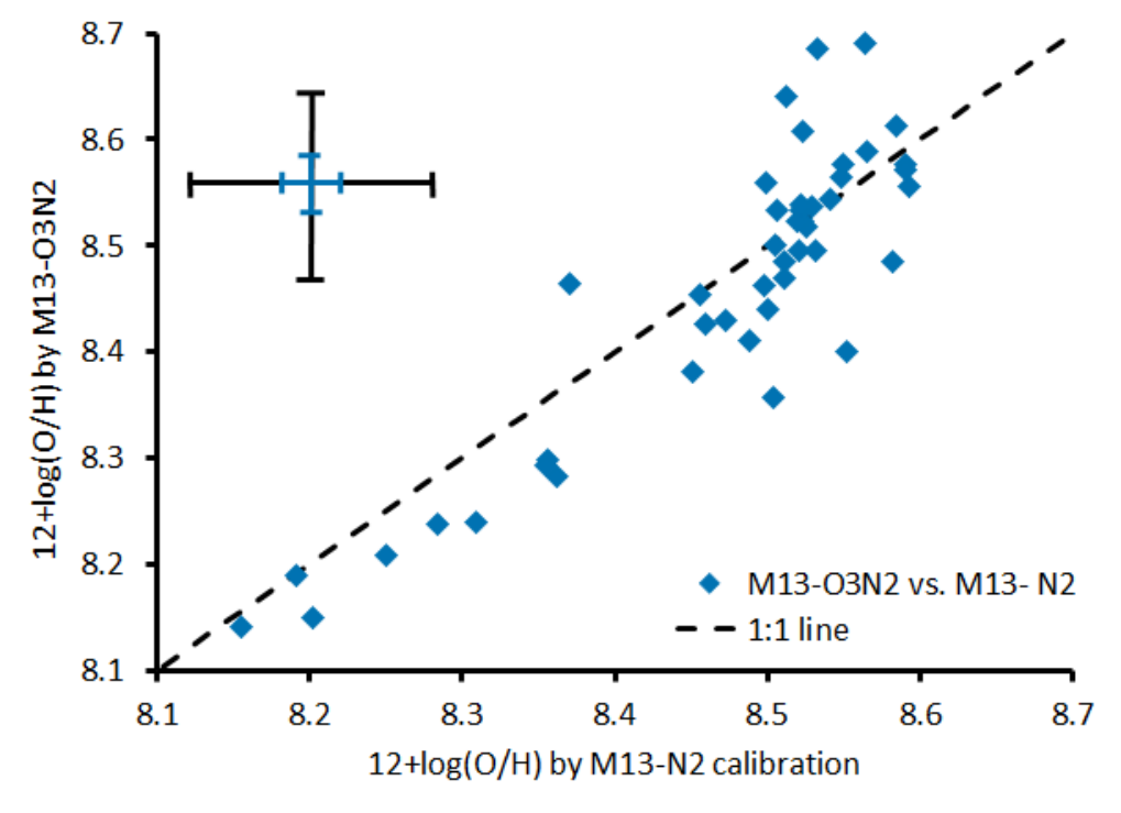
To test the consistency between the two calibrations (M13-O3N2 and M13-N2) we compare the metallicity of each SN calculated with each calibration; the results are presented in Figure 7. It is clear that there is generally a good linear agreement between the calibrations (linear regression coefficient 76%) but an increasing scatter with increasing metallicity is present. This scatter may be caused by the relatively small number of targets in the lower metallicity range and/or by the limitations of the N2 calibration at higher metallicities.

The differences between the N2 and the O3N2 results may have a physical background. As highlighted by e.g. Pettini & Pagel 2004 and Marino et al. 2013, the [N ii] line saturates for metallicities greater than solar metallicity (12 + log(O/H) = 8.69, Asplund et al. 2009) while the [O iii] line does not. Consequently, the N2 calibration should be unreliable for high metallicities as it relies just on [N ii]. This larger uncertainty of the N2 calibration at high metallicities is consistent with the larger scatter at higher metallicities in Figure 7. However, the spread, potentially indicating saturation effects, starts at about 8.5 dex, well below solar metallicity. The N2 calibration is known to produce scatter above solar metallicity but our work suggests that these effects could be present at lower metallicities of 8.5 dex, however given the large calibration errors it is difficult to draw any firm conclusions.
The number of outliers (6% of total sample) is too small to explain the differences between the N2 and O3N2 results because the CDFs do not change significantly if the outliers are removed. The observed trends between SN subtypes in the CDFs are most likely not caused by an improper application of the strong emission lines methods.
5.4 Monte-Carlo Simulations
Results of the statistical significance tests presented in Table 4 are based on values of the metallicities for environment of the three SN subtypes. These values suffer from large uncertainties of 0.16 dex and 0.18 dex for M13-N2 and M13-O3N2, respectively and can ultimately lead to a large range of absolute values and thus a range of p-values. For example, Leloudas et al. 2011 performed Monte-Carlo (MC) simulations perturbing the metallicity around the mean value and found 0.007p0.483 at a 68% confidence interval. Monte-Carlo (MC) simulations have been applied to estimate the sensitivity of the p-values of the KS- and AD-test to the uncertainties of the metallicity results from the INT data.
-
The MC simulations were done by a simple algorithm as follows:
-
take the vector a1 of the nominal metallicity values of the first SN type and add a random vector (representing the possible effect of the uncertainty), where each vector component is randomly drawn from a Gaussian distribution with mean=0.0 and standard deviation sigma=sd1;
-
take the vector a2 of the nominal metallicity values of the second SN type and add a random vector, where each vector component is randomly drawn from a Gaussian distribution with mean=0.0 and sigma=sd2;
-
apply the KS- and the AD-test to the vector a1 and a2;
-
repeat the three steps above for a large number N;
-
create the histogram of the N calculated p-values of the KS- and of the AD-test.
The number N was chosen to be 20000 as a reasonable choice between significance of the MC results and the required time. The standard deviations sd1 and sd2 were constant for each particular MC simulation, but they were changed between 0.0 dex and 0.18 dex (maximum uncertainty of the calibrations) for different MC runs to evaluate the distribution of the p-values at different uncertainties. As in Section 4, the ‘R’ package implementations of the KS- and the AD-test have been used to perform the tests in the MC runs.
The distributions of resulting p-values are presented in Figure 8 and the range of possible p-values increases as the uncertainty increases. For observational uncertainties of 0.04 dex p-values up to 0.5 for the KS-test are possible, which is similar to the range found by Leloudas et al. 2011. For the AD-test, p-values range between 0 and 0.6. However, for the uncertainties given by the strong emission line calibrations (0.16 dex), all p-values between 0 and 1 are possible in both the KS- and AD-tests independent of the samples used. There is a clear qualitative difference between the distributions of p-values of the KS- and the AD-test: the KS-test distribution tends to a more multimodal distribution, the AD-test to a more continuous distribution of the p-values (see Figure 8 for an example). We suggest that this could be due to use of a single supremum value in the KS-test in combination with the relatively small samples. However, this is beyond the scope of this paper. Taking into account the high sensitivity of the p-values to uncertainties, the application of the KS-test and/or AD-test is questioned if the samples under test suffer large uncertainties.
5.5 Constraints for Type Ibc Progenitors
The results for mean metallicities in Table 3 show no statistically significant difference between the three SN subtypes which is in a good agreement with previous studies by Anderson et al. 2010, Galbany et al. 2016c, Kuncarayakti et al. 2018, Leloudas et al. 2011 and Sanders et al. 2012. The results of Modjaz et al. 2011 and Kuncarayakti et al. 2013b, which found higher metallicities for Type Ic SNe compared with Type Ib SNe, could not be confirmed. As discussed in Section 4, there is only a slight metallicity difference of 0.08 dex between the Type Ibc and Type IIP SN for the M13-O3N2 calibration. This tendency is confirmed in the corresponding CDF (Figure 3), but the KS- and the AD-test in Section 4 revealed no statistical significance between the parent population of different SN subtypes in agreement with the KS-test results of Anderson et al. 2010, Galbany et al. 2016c, Kuncarayakti et al. 2018, Leloudas et al. 2011, Sanders et al. 2012 and the AD-test results of Galbany et al. 2018.
However, the MC simulation results of KS- and AD-test highlight the limitations of these two statistical tests as a result of the large uncertainties associated with the calibrations themselves; this is consistent with the findings of Leloudas et al. 2011 for the KS-test. Additionally, as for all statistical tests, if the test does not reject the null hypothesis, this does not conclusively mean that the alternative hypothesis is wrong.


| SN | N(N2) | M13-N2 | N(O3N2) | M13-O3N2 | ||
|---|---|---|---|---|---|---|
| type | [12+log(O/H)] | [12+log(O/H)] | ||||
| mean | mean | |||||
| Ib | 31 | 8.52 | 0.06 | 26 | 8.50 | 0.06 |
| Ic | 40 | 8.49 | 0.13 | 38 | 8.47 | 0.14 |
| IIP | 60 | 8.49 | 0.13 | 49 | 8.44 | 0.12 |
| all | 131 | 8.50 | 0.12 | 113 | 8.46 | 0.12 |
For example, the distribution of Type Ib SNe metallicity environments is narrower than Type Ic and IIP (Figure 3). This finding is consistent with the CDFs of Kuncarayakti et al. 2018 and Galbany et al. 2018 giving some evidence of different physical qualities of Type Ib environments which implies different physical progenitors of Type Ib SN compared to Type Ic and IIP. To test this further, results for the Type Ib/Ic/IIP sub-sample77 7 the data of the total sample of Galbany et al. 2018 have been downloaded from https://iopscience.iop.org/article/10.3847/1538-4357/aaaf20 in Galbany et al. 2018 have been used. This sub-sample consists of 19 Type Ib, 20 Type Ic and 31 Type IIP, and it is almost completely distinct from our sample (only 5 IIP, 2 Ib and 1 Ic SNe are common in both samples). Figure 10 compares the Type Ib and Ic CDFs from this work with the corresponding CDFs of the Type Ib and Ic sub-sample of Galbany et al. 2018 for the M13-O3N2 calibration. The narrow Type Ib distribution and the broader Type Ic distribution starting at low metallicities seen in our work are confirmed by the Galbany et al. 2018 sub-sample.
| KS-test | AD-test | |||
| SN | M13-N2 | M13-O3N2 | M13-N2 | M13-O3N2 |
| types | p-value | p-value | p-value | p-value |
| Ib-Ic | 0.245 | 0.311 | 0.138 | 0.086 |
| Ib-IIP | 0.120 | 0.027 | 0.077 | 0.020 |
| Ic-IIP | 0.788 | 0.189 | 0.853 | 0.165 |
| Ib-(Ic+IIP) | 0.088 | 0.056 | 0.082 | 0.037 |
Figure 10 shows the M13-O3N2 calibration CDFs of the combined sample from this work (including the 4 targets of Table A.3) plus the Galbany et al. 2018 sub-sample. The combined M13-O3N2 sample consists of 26 Type Ib, 38 Type Ic and 49 Type IIP. It confirms our CDFs of Figure 3 both qualitatively and quantitatively with a higher statistical significance because of the considerably larger sample size. The mean metallicities and the standard deviations of the combined sample are shown in Table 6. The smaller standard deviation of the Type Ib results compared with Types Ic and IIP, as seen in Table 3, is confirmed in the combined sample. The KS- and AD-test of the combined sample (Table 7) indicate a statistically significant difference of the O3N2 results between Type Ib vs. IIP and Type Ib vs. Ic+IIP at a significance level of 5%. All other test results indicate no significant differences below a 5% level.
We note that these statistical tests are still subject to the large calibration uncertainties as discussed in Section 5.4. However, accepting the limitations of the KS- and AD-tests, is it possible to draw any conclusions regarding the progenitors of the different SN subtypes based on the CDF’s and subsequent analysis? If the differences are indeed real, what do they represent?
Single massive stars have less physical parameters determining their mass loss (essentially initial mass, metallicity, rotation and magnetic field). Compared with single stars, compact binaries have additional orbital and evolutionary parameters of the companion influencing the mass-loss/overflow rate. For instance, a massive star with mass and metallicity to evolve as single star to a Type Ib SN, can evolve to Type Ic by additional mass-loss to its companion in a compact binary system - the number of evolutionary pathways of the massive star has been increased by the companion. Consequently, the larger number of physical parameters induces the expectation of a larger scatter (e.g. Xiao et al. 2019) and consequently of broader CDFs in metallicity for the binary scenario. Consequently, the narrower Type Ib CDFs seen in the Figures 3, 10 and 10 may be an indication that the single massive progenitor star fraction for Type Ib is larger than for Type Ic.
Type Ic SNe have a broad distribution starting at low metallicities, where it closely matches the Type IIP distribution for 12log(O/H) 8.3. Besides the broad distribution, the low metallicity limit for Type Ic is a second indication of a significant binary fraction of Type Ic SNe progenitors. Stripping H- and He-shells at low metallicities by stellar winds only is unlikely because the mass loss strongly depends on metallicity (the higher metallicity the stronger mass loss; e.g. Vink & Gräfener 2012). Thus, the binary scenario is favoured as the mass stripping mechanism at low metallicities. This conclusion is consistent with Smith et al. 2011a, who derived, based on standard IMFs and the observed fractions of core-collapse SNe, the necessity of binary progenitors. However, the single massive star formation channel for Type Ic SNe cannot be ruled out from our data and a mixture of both formation channels is likely.
While the agreement of the Type Ic and IIP CDFs at lower metallicity (e.g. this work; Galbany et al. 2018; Kuncarayakti et al. 2018) might seem contradictory given the single, massive nature of confirmed IIP progenitors (Smartt 2009; Van Dyk 2017), Type IIP progenitors have no need to lose their outer envelope allowing a broader range of masses and metallicities for single massive progenitors of Type IIP SN compared with Type Ib.
All constraints drawn above are not as distinctive for the N2 calibration results. However, it is reassuring that the CDFs created from data of the independent investigations by Galbany et al. 2018 are very similar (Figure 10) to ours and that the CDFs of the combined sample (Figure 10) still show the distinctive features. The combined samples produce a statistically significant rejection of our null-hypothesis for Ib-IIP SNe with p = 0.027 and p = 0.020 (see Table 7) for the KS- and AD-tests, respectively, as a result of increased sample size. More observations of SNe environments and metallicity calibrations with significantly lower uncertainties, supported by direct measurements of metallicities via massive stars (Davies et al. 2017) are still required to investigate all SN subtypes thoroughly and improve our understanding of core-collapse SNe progenitors.
6 Summary and Conclusions
This work calculates and compares the metallicities of environments of Type IIP, Type Ib and Type Ic SNe within a luminosity distance of 30 Mpc by the strong emission line method. 76 targets were observed with INT/IDS and metallicity was measured for 65 of these using the N2 and O3N2 calibrations. The CDFs based on O3N2 calibration exhibit distinct features: narrow Type Ib distribution, Type Ic at low metallicities and higher mean metallicities for Ibc SN compared to IIP. However, taking into account measurement errors, the statistical tests (KS-test and AD-test) are formally unable to reject the null hypothesis that the different SN types come from the same parent population.
The results of our analysis have been confirmed and strengthened by the CDFs created from the Type Ib/Ic/IIP sample of Galbany et al. 2018 as well as by the CDFs of the large combined sample of this work and the Galbany et al. 2018 sub-sample. For the combined sample, both statistical tests indicate a statistically significant difference between the Type Ib and Type IIP M13-O3N2 results at 5% significance level. This suggests that Ib and IIP SN do indeed have different progenitor populations.
This statistical result combined with the apparent shapes of CDFs (see Figure 10), might be explained by a significant fraction of single massive stars as Type Ib progenitors and suggests a significant fraction of compact binaries as progenitors of Type Ic SNe because they are present in low metallicity environments. Despite the large sample size of observed SNe environments these indications need further investigation with more observations of SNe environments in future work, to verify the significance of our results.
MC simulations have shown that the large calibration uncertainties have a significant effect on the range of p-values possible for both the KS- and AD-tests. These uncertainties must be reduced through improved calibrations and investigation of the saturation of the [N ii] emission line.
Acknowledgements
The work presented is based on observations made with the Isaac Newton Telescope. The Isaac Newton Telescope is operated on the island of La Palma by the Isaac Newton Group of Telescopes in the Spanish Observatorio del Roque de los Muchachos of the Instituto de Astrofísica de Canarias. We would like to thank Isaac Newton Group of Telescopes staff and our co-observers A. Brocklebank, T. Davison, A. de Burgos, L. Holden, D. Nespral, S. Percival, T. Wilson, and T. Zegmott for their contributions to the observation data. J. L. Pledger, A. E. Sansom and S.M. Habergham-Mawson acknowledge financial support through the Panel for the Application of Telescope Time (PATT) travel grant (IDs ST/S005307/1 and ST/M00211X/1). Supernova data have been obtained from the Open Supernova Catalogue currently maintained by James Guillochon and Jerod Parrent. Host galaxy data have been obtained from the NASA/IPAC Extragalactic Database (NED), which is operated by the Jet Propulsion Laboratory, California Institute of Technology, under contract with the National Aeronautics and Space Administration. The research has made use of tools created by hard work of the astronomical community, acknowledged here by tool name and URL: IRAF (https://iraf.net), Starlink (http://starlink.eao.hawaii.edu/starlink), Hyperleda (http://leda.univ-lyon1.fr), ’R’-project (http://www.R-project.org), PPXF (https://pypi.org/project/ppxf), MILES stellar library (http://miles.iac.es/pages/stellar-libraries/miles-library.php)
Data Availability
The data underlying this article will be shared on reasonable request to the corresponding author.
References
- Aldering et al. (1994) Aldering G., Humphreys R. M., Richmond M., 1994, AJ, 107, 662
- Anderson & James (2008) Anderson J. P., James P. A., 2008, MNRAS, 390, 1527
- Anderson & James (2009) Anderson J. P., James P. A., 2009, MNRAS, 399, 559
- Anderson et al. (2010) Anderson J. P., Covarrubias R. A., James P. A., Hamuy M., Habergham S. M., 2010, MNRAS, 407, 2660
- Anderson et al. (2014) Anderson J. P., et al., 2014, ApJ, 786, 67
- Anderson et al. (2015) Anderson J. P., James P. A., Habergham S. M., Galbany L., Kuncarayakti H., 2015, PASA, 32, 19A
- Arcavi et al. (2010) Arcavi I., et al., 2010, ApJ, 721, 777
- Asplund et al. (2009) Asplund M., Grevesse N., Sauval A. J., Scott P., 2009, ARA&A, 47, 481
- Baldwin et al. (1981) Baldwin J. A., Phillips M. M., Terlevich R., 1981, PASP, 93, 5
- Barth et al. (1996) Barth A. J., van Dyk S. D., Filippenko A. V., Leibundgut B., Richmond M. W., 1996, AJ, 111, 2047
- Benetti et al. (2016) Benetti S., et al., 2016, MNRAS, 456, 3296
- Bersten et al. (2014) Bersten M. C., et al., 2014, AJ, 148, 68
- Boissier & Prantzos (2009) Boissier S., Prantzos N., 2009, A&A, 503, 137
- Cao et al. (2013) Cao Y., et al., 2013, ApJ, 775, L7
- Cappellari (2017) Cappellari M., 2017, MNRAS, 466, 798
- Cappellari & Emsellem (2004) Cappellari M., Emsellem E., 2004, PASP, 116, 138
- Chen (2021) Chen K.-J., 2021, IJMPD, 30, 2130001
- Crockett et al. (2007) Crockett R. M., et al., 2007, MNRAS, 381, 835
- Crockett et al. (2008) Crockett R. M., et al., 2008, MNRAS, 391, L5
- Crowther (2007) Crowther P. A., 2007, ARA&A, 45, 177
- Crowther (2013) Crowther P. A., 2013, MNRAS, 428, 1927
- Currie et al. (2014) Currie M. J., Berry D. S., Jenness T., Gibb A. G., Bell G. S., Draper P. W., 2014, ASPC, 485, 391
- Davies et al. (2017) Davies B., et al., 2017, ApJ, 847, 112
- Dessart et al. (2011) Dessart L., Hillier D. J., Livne E., Yoon S.-C., Woosley S., Waldman R., Langer N., 2011, MNRAS, 414, 2985
- Dowd (2018) Dowd C., 2018, twosamples: Fast Permutation Based Two Sample Tests. https://CRAN.R-project.org/package=twosamples
- Eldridge & Maund (2016) Eldridge J. J., Maund J. R., 2016, MNRAS, 461, L117
- Eldridge et al. (2008) Eldridge J. J., Izzard R. G., Tout C. A., 2008, MNRAS, 384, 1109
- Eldridge et al. (2015) Eldridge J. J., Fraser M., Maund J. R., Smartt S. J., 2015, MNRAS, 446, 2689
- Elias-Rosa et al. (2010) Elias-Rosa N., et al., 2010, ApJ, 714, L254
- Elias-Rosa et al. (2011) Elias-Rosa N., et al., 2011, AJ, 742, 6
- Elias-Rosa et al. (2013) Elias-Rosa N., et al., 2013, MNRAS, 436, L109
- Fang & Maeda (2018) Fang Q., Maeda K., 2018, ApJ, 864, 47
- Filippenko (1997) Filippenko A. V., 1997, ARA&A, 35, 309
- Filippenko et al. (2003) Filippenko A. V., Chornock R., Swift B., Modjaz M., Simcoe R., Rauch M., 2003, IAUC, 8159, 2
- Fitzpatrick (1985) Fitzpatrick E. L., 1985, ApJ, 299, 219
- Folatelli et al. (2016) Folatelli G., et al., 2016, ApJL, 825, L22
- Foley et al. (2011) Foley R. J., Berger E., Fox O., Levesque E. M., Challis P. J., Ivans I. I., Rhoads J. E., Soderberg A. M., 2011, AJ, 732, 32
- Fremling et al. (2014) Fremling C., et al., 2014, A&A, 565, A114
- Fruchter et al. (2006) Fruchter A. S., et al., 2006, Nature, 441, 463
- Gal-Yam (2019) Gal-Yam A., 2019, ARA&A, 57, 305
- Gal-Yam & Leonard (2009) Gal-Yam A., Leonard D. C., 2009, Nature, 458, 865
- Gal-Yam et al. (2005) Gal-Yam A., et al., 2005, ApJ, 630, L29
- Galbany et al. (2016a) Galbany L., et al., 2016a, AJ, 151, 33
- Galbany et al. (2016b) Galbany L., et al., 2016b, MNRAS, 455, 4087
- Galbany et al. (2016c) Galbany L., et al., 2016c, A&A, 591, A48
- Galbany et al. (2018) Galbany L., et al., 2018, ApJ, 855, 107
- Graham (2019) Graham J. F., 2019, arXiv e-prints, p. arXiv:1905.13197
- Groh et al. (2013) Groh J. H., Georgy C., Ekstrom S., 2013, A&A, 558, L1
- Guillochon et al. (2017) Guillochon J., Parrent J., Kelley L. Z., Margutti R., 2017, ApJ, 835, 64
- Gutiérrez et al. (2017) Gutiérrez C. P., et al., 2017, ApJ, 850, 89
- Hakobyan et al. (2014) Hakobyan A. A., et al., 2014, MNRAS, 444, 2428
- Hakobyan et al. (2016) Hakobyan A. A., et al., 2016, MNRAS, 456, 2848
- Helou et al. (1991) Helou G., Madore B. F., Schmitz M., Bicay M. D., Wu X., Bennett J., 1991, ASSL, 171, 89
- Henry & Worthey (1999) Henry R. B. C., Worthey G., 1999, PASP, 111, 919
- Hirai (2017) Hirai R., 2017, MNRAS, 466, 3775
- Hummer & Storey (1987) Hummer D. G., Storey P. J., 1987, MNRAS, 224, 801
- James & Anderson (2006) James P. A., Anderson J. P., 2006, A&A, 453, 57
- Johnson et al. (2017) Johnson S. A., Kochanek C. S., Adams S. M., 2017, MNRAS, 472, 3115
- Kelly & Kirshner (2012) Kelly P. L., Kirshner R. P., 2012, ApJ, 759, 107
- Kewley & Ellison (2008) Kewley L. J., Ellison S. L., 2008, ApJ, 681, 1183
- Kewley et al. (2001) Kewley L. J., Dopita M. A., Sutherland R. S., Heisler C. A., Trevena J., 2001, ApJ, 556, 121
- Kewley et al. (2019) Kewley L. J., Nicholls D. C., Sutherland R. S., 2019, ARA&A, 57, 511
- Kilpatrick et al. (2018) Kilpatrick C. D., et al., 2018, MNRAS, 480, 2072
- Kilpatrick et al. (2021) Kilpatrick C. D., et al., 2021, MNRAS, 504, 2073
- Krühler et al. (2017) Krühler T., Kuncarayakti H., Schady P., Anderson J. P., Galbany L., Gensior J., 2017, A&A, 602, A85
- Kudritzki & Puls (2000) Kudritzki R.-P., Puls J., 2000, ARA&A, 38, 613
- Kuncarayakti et al. (2013a) Kuncarayakti H., et al., 2013a, AJ, 146, 31
- Kuncarayakti et al. (2013b) Kuncarayakti H., et al., 2013b, AJ, 146, 30
- Kuncarayakti et al. (2015) Kuncarayakti H., et al., 2015, A&A, 579, A95
- Kuncarayakti et al. (2018) Kuncarayakti H., et al., 2018, A&A, 613, A35
- Leloudas et al. (2011) Leloudas G., et al., 2011, A&A, 530, A95
- Lunnan et al. (2017) Lunnan R., et al., 2017, ApJ, 836, 60
- Lyman et al. (2013) Lyman J. D., James P. A., Perets H. B., Anderson J. P., Gal-Yam A., Mazzali P., Percival S. M., 2013, MNRAS, 434, 527
- Makarov et al. (2014) Makarov D., Prugniel P., Terekhova N., Courtois H., Vauglin I., 2014, A&A, 570, A13
- Maoz et al. (2014) Maoz D., Mannucci F., Nelemans G., 2014, ARA&A, 52, 107
- Marino et al. (2013) Marino R. A., et al., 2013, A&A, 559, A114
- Marsaglia et al. (2003) Marsaglia G., Tsang W. W., Wang J., 2003, JSS, 8, 1
- Massey (1952) Massey F. J., 1952, AoMS, 23, 435
- Maund (2018) Maund J. R., 2018, MNRAS, 476, 2629
- Maund & Smartt (2005) Maund J. R., Smartt S. J., 2005, MNRAS, 360, 288
- Maund et al. (2004) Maund J. R., Smartt S. J., Kudritzki R. P., Podsiadlowski P., Gilmore G. F., 2004, Nature, 427, 129
- Maund et al. (2005) Maund J. R., Smartt S. J., Schweizer F., 2005, ApJ, 630, L33
- Maund et al. (2011) Maund J. R., et al., 2011, ApJ, 739, L37
- Mazzali et al. (2002) Mazzali P. A., et al., 2002, ApJ, 572, L61
- Modjaz et al. (2008) Modjaz M., et al., 2008, AJ, 135, 1136
- Modjaz et al. (2011) Modjaz M., Kewley L., Bloom J. S., Filippenko A. V., Perley D., Silverman J. M., 2011, ApJ, 731, L4
- Osterbrock & Ferland (2006) Osterbrock D. E., Ferland G. J., 2006, Astrophysics of gaseous nebulae and active galactic nuclei, 2nd ed edn. University Science Books, Sausalito, Calif
- Pandey et al. (2021) Pandey S. B., et al., 2021, arXiv:astro-ph/2106.15856
- Pettini & Pagel (2004) Pettini M., Pagel B. E. J., 2004, MNRAS, 348, L59
- Pettitt (1976) Pettitt A. N., 1976, Biometrika, 63, 161
- Podsiadlowski et al. (1992) Podsiadlowski P., Joss P. C., Hsu J. J. L., 1992, ApJ, 391, 246
- Prantzos & Boissier (2003) Prantzos N., Boissier S., 2003, A&A, 406, 259
- Press (1988) Press W. H., ed. 1988, Numerical recipes in C: the art of scientific computing. Cambridge University Press, Cambridge [Cambridgeshire] ; New York
- Prieto et al. (2008) Prieto J. L., Stanek K. Z., Beacom J. F., 2008, ApJ, 673, 999
- Sanders et al. (2012) Sanders N. E., et al., 2012, ApJ, 758, 132
- Sanders et al. (2015) Sanders N. E., et al., 2015, ApJ, 799, 208
- Schady et al. (2019) Schady P., Eldridge J. J., Anderson J., Chen T.-W., Galbany L., Kuncarayakti H., Xiao L., 2019, MNRAS, 490, 4515
- Schlafly & Finkbeiner (2011) Schlafly E. F., Finkbeiner D. P., 2011, ApJ, 737, 103
- Schlegel (1990) Schlegel E. M., 1990, MNRAS, 244, 269
- Shen et al. (2019) Shen K. J., Quataert E., Pakmor R., 2019, ApJ, 887, 180
- Smartt (2009) Smartt S. J., 2009, ARA&A, 47, 63
- Smartt (2015) Smartt S. J., 2015, PASA, 32, e016
- Smartt et al. (2002) Smartt S. J., Vreeswijk P. M., Ramirez-Ruiz E., Gilmore G. F., Meikle W. P. S., Ferguson A. M. N., Knapen J. H., 2002, ApJ, 572, L147
- Smith (2014) Smith N., 2014, ARA&A, 52, 487
- Smith et al. (2011a) Smith N., Li W., Filippenko A. V., Chornock R., 2011a, MNRAS, 412, 1522
- Smith et al. (2011b) Smith N., et al., 2011b, AJ, 732, 63
- Taddia et al. (2013a) Taddia F., et al., 2013a, A&A, 555, A10
- Taddia et al. (2013b) Taddia F., et al., 2013b, A&A, 558, A143
- Taddia et al. (2015) Taddia F., et al., 2015, A&A, 580, A131
- Taddia et al. (2016) Taddia F., et al., 2016, A&A, 587, L7
- Taddia et al. (2019) Taddia F., et al., 2019, A&A, 621, A71
- Tartaglia et al. (2017) Tartaglia L., et al., 2017, ApJ, 836, L12
- Teffs et al. (2021) Teffs J. J., Prentice S. J., Mazzali P. A., Ashall C., 2021, MNRAS, 502, 3829
- Tody (1986) Tody D., 1986, SPIE, 627, 733
- Turatto (2003) Turatto M., 2003, arXiv:astro-ph/0301107
- Valenti et al. (2011) Valenti S., et al., 2011, MNRAS, 416, 3138
- Valenti et al. (2016) Valenti S., et al., 2016, MNRAS, 459, 3939
- Van Dyk (2017) Van Dyk S. D., 2017, RSPTA, 375, 20160277
- Van Dyk & Schuyler (1992) Van Dyk S. D., Schuyler D., 1992, AJ, 103, 1788
- Van Dyk et al. (2002) Van Dyk S. D., Garnavich P. M., Filippenko A. V., Höflich P., Kirshner R. P., Kurucz R. L., Challis P., 2002, PASP, 114, 1322
- Van Dyk et al. (2011) Van Dyk S. D., et al., 2011, ApJ, 741, L28
- Van Dyk et al. (2014) Van Dyk S. D., et al., 2014, AJ, 147, 37
- Van Dyk et al. (2016) Van Dyk S. D., de Mink S. E., Zapartas E., 2016, ApJ, 818, 75
- Van Dyk et al. (2018) Van Dyk S. D., et al., 2018, ApJ, 860, 90
- Vazdekis et al. (2010) Vazdekis A., Sánchez-Blázquez P., Falcón-Barroso J., Cenarro A. J., Beasley M. A., Cardiel N., Gorgas J., Peletier R. F., 2010, MNRAS, 404, 1639
- Vink & Gräfener (2012) Vink J. S., Gräfener G., 2012, ApJ, 751, L34
- Vink & Sander (2021) Vink J. S., Sander A. A. C., 2021, MNRAS, 504, 2051
- Vink & de Koter (2005) Vink J. S., de Koter A., 2005, A&A, 442, 587
- Woosley & Bloom (2006) Woosley S. E., Bloom J. S., 2006, ARA&A, 44, 507
- Xiang et al. (2019) Xiang D., et al., 2019, ApJ, 871, 176
- Xiao et al. (2019) Xiao L., Galbany L., Eldridge J. J., Stanway E. R., 2019, MNRAS, 482, 384
- Yoon et al. (2010) Yoon S.-C., Woosley S. E., Langer N., 2010, ApJ, 725, 940
Appendix
| target | type | host | host type | DL | MV | PA | dC | N | Exp. time |
|---|---|---|---|---|---|---|---|---|---|
| [Mpc] | [mag] | [°] | [″] | [sec] | |||||
| 1995bb | Ib/c | PGC1409128 | Irr? | 25.8 | - | 87.6 | 9.38 | 1 | 4800 |
| 1998bv | IIP | HS1035+4758 | ? | 23.4 | -16.0 | 215.8 | 5.18 | 1 | 3600 |
| 1998dl | IIP | NGC1084 | SA(s)c | 16.7 | -21.8 | 54.1 | 28.82 | 1 | 3600 |
| 1999eh | Ib | NGC2770 | SA(s)c | 26.0 | -21.7 | 238.0 | 15.27 | 1 | 3600 |
| 1999em | IIP | NGC1637 | SAB(rs)c | 7.7 | -20.6 | 227.0 | 23.76 | 1 | 3600 |
| 1999ev | IIP | NGC4274 | SB(r)ab | 21.0 | -21.7 | 315.6 | 42.29 | 1 | 3600 |
| 1999gi | IIP | NGC3184 | SAB(rs)cd | 11.0 | -21.0 | 358.5 | 61.22 | 1 | 4000 |
| 2000ds | Ib | NGC2768 | E6 | 17.0 | -21.7 | 196.5 | 33.17 | 2 | 7200 |
| 2000ew | Ic | NGC3810 | SA(rs)c | 16.0 | -21.4 | 187.5 | 20.27 | 1 | 3600 |
| 2001B | Ib | IC391 | SA(s)c | 25.0 | -20.4 | 238.5 | 6.70 | 3 | 10800 |
| 2001ci | Ic | NGC3079 | SB(s)c | 15.0 | -22.1 | 351.8 | 27.88 | 2 | 7200 |
| 2001fv | IIP | NGC3512 | SAB(rs)c | 25.0 | -20.5 | 223.5 | 23.85 | 1 | 4200 |
| 2002hh | IIP | NGC6946 | SAB(rs)cd | 4.7 | -14.8 | 207.5 | 129.63 | 1 | 3600 |
| 2002ji | Ib | NGC3655 | SA(s)c | 26.0 | -21.7 | 236.1 | 25.11 | 1 | 3600 |
| 2002jz | Ic | UGC2984 | SBdm | 22.9 | - | 197.5 | 3.88 | 2 | 7200 |
| 2003gd | IIP | NGC628 | SA(s)c | 3.4 | -20.4 | 175.6 | 159.57 | 1 | 3600 |
| 2003ie | IIP | NGC4051 | SAB(rs)bc | 13.0 | -21.3 | 101.4 | 93.26 | 1 | 1200 |
| 2003J | IIP | NGC4157 | SAB(s)b | 15.7 | -22.0 | 242.5 | 71.89 | 1 | 5400 |
| 2003Z | IIP | NGC2742 | SA(s)c | 20.0 | -21.6 | 346.3 | 32.42 | 1 | 5400 |
| 2004A | IIP | NGC6207 | SA(s)c | 20.0 | -20.5 | 305.7 | 26.59 | 1 | 3600 |
| 2004ao | Ib | UGC10862 | SB(rs)c | 26.0 | -19.1 | 165.3 | 26.36 | 2 | 7200 |
| 2004bm | Ic | NGC3437 | SAB(rs)c | 21.0 | -21.3 | 296.1 | 5.69 | 1 | 3600 |
| 2004C | Ic | NGC3683 | SB(s)c | 35.0 | -20.8 | 303.3 | 20.40 | 1 | 3600 |
| 2004dg | IIP | NGC5806 | SAB(s)b | 22.0 | -22.0 | 261.0 | 21.85 | 1 | 3600 |
| 2004dj | IIP | NGC2403 | SAB(s)cd | 3.5 | -19.4 | 94.0 | 159.14 | 1 | 3600 |
| 2004dk | Ib | NGC6118 | SA(s)cd | 20.0 | -21.8 | 6.6 | 42.99 | 1 | 3600 |
| 2004ez | IIP | NGC3430 | SAB(rs)c | 26.0 | -21.7 | 68.8 | 50.08 | 1 | 4600 |
| 2004fc | IIP | NGC701 | SB(rs)c | 19.0 | -20.9 | 19.4 | 2.23 | 1 | 3600 |
| 2004gk | Ic | IC3311 | Sdm | 17.0 | -18.3 | 31.6 | 3.64 | 1 | 3600 |
| 2004gn | Ic | NGC4527 | SAB(s)bc | 12.6 | -20.7 | 68.9 | 59.43 | 2 | 7200 |
| 2004gq | Ib | NGC1832 | SB(r)bc | 16.0 | -21.7 | 45.0 | 30.83 | 1 | 3600 |
| 2004gt | Ic | NGC4038 | SB(s)m | 16.0 | -21.8 | 255.4 | 38.57 | 1 | 3600 |
| 2005ad | IIP | NGC941 | SAB(rs)c | 20.0 | -19.1 | 28.3 | 52.23 | 1 | 3600 |
| 2005ay | IIP | NGC3938 | SA(s)c | 18.0 | -20.7 | 194.2 | 58.38 | 1 | 3600 |
| 2005cs | IIP | NGC5194 | SA(s)bc | 6.1 | -20.9 | 179.3 | 67.30 | 1 | 3600 |
| 2005cz | Ib | NGC4589 | E2 | 20.0 | -21.6 | 119.2 | 13.34 | 1 | 3800 |
| 2005kl | Ic | NGC4369 | SA(rs)a | 21.0 | -21.1 | 306.7 | 7.52 | 1 | 4800 |
| 2005V | Ib/c | NGC2146 | SB(s)ab | 17.0 | -22.1 | 24.8 | 4.19 | 1 | 3600 |
| 2006bp | IIP | NGC3953 | SB(r)bc | 17.0 | -22.3 | 33.9 | 112.49 | 1 | 4000 |
| 2007aa | IIP | NGC4030 | SA(s)bc | 23.0 | -22.3 | 41.9 | 91.88 | 1 | 3600 |
| 2007av | IIP | NGC3279 | Sd | 29.0 | -21.8 | 155.0 | 12.90 | 2 | 7800 |
| 2007C | Ib | NGC4981 | SAB(r)bc | 21.0 | -21.5 | 157.9 | 23.75 | 1 | 4200 |
| 2007gr | Ic | NGC1058 | SA(rs)c | 10.0 | -17.5 | 303.1 | 28.75 | 3 | 10800 |
| 2007od | IIP | UGC12846 | Sm | 24.0 | - | 132.7 | 51.90 | 1 | 3600 |
| 2008D | Ib | NGC2770 | SA(s)c | 26.0 | -21.7 | 325.3 | 67.27 | 2 | 7800 |
| 2008X | IIP | NGC4141 | SBcd | 28.0 | -18.9 | 60.1 | 9.22 | 1 | 3600 |
| 2009em | Ic | NGC157 | SAB(rs)bc | 23.0 | -21.7 | 251.8 | 33.90 | 1 | 3600 |
| 2009js | IIP | NGC918 | SAB(rs)c | 16.0 | -21.4 | 240.6 | 41.15 | 1 | 3600 |
| 2010br | Ib/c | NGC4051 | SAB(rs)bc | 13.0 | -21.3 | 124.4 | 17.50 | 1 | 4000 |
| 2010io | Ic | UGC4543 | SAdm | 29.0 | -18.5 | 333.0 | 8.98 | 3 | 8400 |
| 2011ck | IIP | NGC5425 | Sd | 30.7 | -19.2 | 297.0 | 16.30 | 1 | 3600 |
| 2011dq | IIP | NGC337 | SB(s)d | 24.4 | -21.1 | 300.4 | 40.51 | 1 | 3600 |
| 2011jm | Ic | NGC4809 | Im | 13.8 | -17.3 | 93.8 | 1.50 | 1 | 3600 |
| 2012A | IIP | NGC3239 | IB(s)m | 8.8 | -19.7 | 133.9 | 49.57 | 1 | 4200 |
| 2012au | Ib | NGC4790 | SB(rs)c | 20.0 | -19.4 | 66.5 | 4.51 | 1 | 4200 |
| 2012bv | IIP | NGC6796 | Sbc | 32.5 | -21.0 | 187.4 | 30.25 | 1 | 4800 |
| 2012cw | Ic | NGC3166 | SAB(rs)a | 19.9 | -22.6 | 46.3 | 48.65 | 2 | 8400 |
| 2012ec | IIP | NGC1084 | SA(s)c | 16.7 | -21.8 | 358.9 | 15.00 | 1 | 3600 |
| 2012fh | Ic | NGC3344 | SAB(r)bc | 8.6 | -20.4 | 160.1 | 118.03 | 1 | 4200 |
| 2012P | Ib/c | NGC5806 | SAB(s)b | 22.0 | -22.0 | 256.5 | 19.73 | 1 | 4000 |
| 2013ab | IIP | NGC5669 | SAB(rs)d | 23.6 | -20.5 | 133.1 | 20.04 | 1 | 3600 |
| 2013bu | IIP | NGC7331 | SA(s)bc | 12.1 | -23.0 | 204.0 | 55.62 | 2 | 8400 |
| 2013dk | Ic | NGC4038 | SB(s)m | 16.0 | -21.8 | 194.6 | 15.81 | 1 | 4200 |
| 2013ej | IIP | NGC628 | SA(s)c | 3.4 | -20.4 | 134.1 | 127.87 | 1 | 4800 |
| 2013ff | Ic | NGC2748 | SAbc | 21.9 | -21.0 | 215.6 | 24.84 | 1 | 3600 |
| 2013ge | Ic | NGC3287 | SB(s)d | 19.3 | -18.4 | 18.7 | 50.56 | 2 | 6600 |
| 2014A | IIP | NGC5054 | SA(s)bc | 27.0 | -21.4 | 57.1 | 14.72 | 1 | 3600 |
| 2014bc | IIP | NGC4258 | SAB(s)bc | 6.6 | -21.9 | 141.7 | 3.44 | 1 | 4200 |
| 2014bi | IIP | NGC4096 | SAB(rs)c | 8.3 | -21.1 | 20.4 | 54.95 | 1 | 4200 |
| 2014C | Ib | NGC7331 | SA(s)bc | 12.1 | -23.0 | 140.6 | 31.19 | 1 | 3600 |
| 2014cx | IIP | NGC337 | SB(s)d | 24.4 | -21.1 | 303.6 | 40.51 | 1 | 3600 |
| 2015aq | IIP | UGC5015 | SABdm | 24.0 | -18.5 | 267.5 | 43.05 | 1 | 4200 |
| 2015V | IIP | UGC11000 | S? | 20.3 | -18.5 | 142.1 | 8.87 | 1 | 3600 |
| 2016bau | Ib | NGC3631 | SA(s)c | 17.1 | -19.5 | 293.5 | 37.95 | 1 | 3600 |
| 2017ein | Ic | NGC3938 | SA(s)c | 18.0 | -20.7 | 74.2 | 42.53 | 1 | 3600 |
| 2017iro | Ib | NGC5480 | SA(s)c | 27.5 | -21.3 | 125.0 | 17.74 | 1 | 3600 |
| target | type | SN RA | SN Dec | M13-N2 | M13-O3N2 | PP04-N2 | PP04-O3N2 |
|---|---|---|---|---|---|---|---|
| [h m s] | [° ′ ″] | 12+log(O/H) | 12+log(O/H) | 12+log(O/H) | 12+log(O/H) | ||
| 1998bv | IIP | 10 38 25.40 | +47 42 32.8 | 8.19 | 8.19 | 8.22 | 8.21 |
| 1998dl | IIP | 02 46 01.47 | -07 34 25.1 | 8.52 | 8.52 | 8.62 | 8.72 |
| 1999eh | Ib | 09 09 32.67 | +33 07 16.9 | 8.50 | - | 8.61 | - |
| 1999em⋆ | IIP | 04 41 27.04 | -02 51 45.2 | 8.77 | - | 8.93 | - |
| 1999gi | IIP | 10 18 16.66 | +41 26 28.2 | 8.42 | - | 8.51 | - |
| 2000ds11 1 classified as Ca-rich and excluded from statistical evalutions (see Section 4)⋆ | Ib | 09 11 36.24 | +60 01 42.2 | 8.85 | - | 9.03 | - |
| 2000ew | Ic | 11 40 58.52 | +11 27 55.9 | 8.50 | 8.71 | 8.60 | 8.99 |
| 2001B | Ib | 04 57 19.24 | +78 11 16.5 | 8.51 | 8.49 | 8.61 | 8.65 |
| 2001ci | Ic | 10 01 57.33 | +55 41 14.6 | 8.59 | 8.57 | 8.71 | 8.79 |
| 2001fv | IIP | 11 04 01.66 | +28 01 55.7 | 8.71 | - | 8.86 | |
| 2002hh | IIP | 20 34 44.29 | +60 07 19.0 | 8.52 | 8.54 | 8.63 | 8.74 |
| 2002ji | Ib | 11 22 53.15 | +16 35 10.0 | 8.53 | 8.54 | 8.64 | 8.74 |
| 2002jz | Ic | 04 13 12.52 | +13 25 07.3 | 8.25 | 8.21 | 8.29 | 8.24 |
| 2003gd | IIP | 01 36 42.65 | +15 44 20.9 | 8.68 | - | 8.83 | - |
| 2003J | IIP | 12 10 57.72 | +50 28 31.8 | 8.67 | - | 8.81 | - |
| 2003Z | IIP | 09 07 32.46 | +60 29 17.5 | 8.55 | 8.40 | 8.66 | 8.53 |
| 2004A | IIP | 16 43 01.90 | +36 50 12.5 | 8.50 | - | 8.59 | - |
| 2004ao | Ib | 17 28 09.35 | +07 24 55.5 | 8.49 | 8.41 | 8.59 | 8.55 |
| 2004bm | Ic | 10 52 35.33 | +22 56 05.5 | 8.56 | 8.69 | 8.68 | 8.97 |
| 2004C | Ic | 11 27 29.72 | +56 52 48.2 | 8.52 | 8.52 | 8.63 | 8.72 |
| 2004dg | IIP | 14 59 58.96 | +01 53 25.6 | 8.53 | 8.68 | 8.64 | 8.96 |
| 2004dj | IIP | 07 37 17.02 | +65 35 57.8 | 8.50 | 8.36 | 8.61 | 8.47 |
| 2004dk | Ib | 16 21 48.93 | -02 16 17.3 | 8.37 | 8.46 | 8.44 | 8.63 |
| 2004fc | IIP | 01 51 03.85 | -09 42 06.9 | 8.55 | 8.56 | 8.66 | 8.78 |
| 2004gk | Ic | 12 25 33.23 | +12 15 40.1 | 8.50 | 8.44 | 8.60 | 8.59 |
| 2004gn | Ic | 12 34 12.10 | +02 39 34.4 | 8.51 | 8.64 | 8.62 | 8.89 |
| 2004gq | Ib | 05 12 04.81 | -15 40 54.2 | 8.55 | 8.58 | 8.66 | 8.80 |
| 2004gt | Ic | 12 01 50.37 | -18 52 12.7 | 8.53 | 8.52 | 8.63 | 8.71 |
| 2005ay | IIP | 11 52 48.07 | +44 06 18.4 | 8.56 | 8.59 | 8.68 | 8.81 |
| 2005cs | IIP | 13 29 52.78 | +47 10 35.7 | 8.44 | - | 8.52 | - |
| 2005kl | Ic | 12 24 35.68 | +39 23 03.5 | 8.51 | 8.53 | 8.61 | 8.73 |
| 2005V | Ib/c | 06 18 38.28 | +78 21 28.8 | 8.59 | 8.56 | 8.71 | 8.76 |
| 2006bp | IIP | 11 53 55.74 | +52 21 09.4 | 8.54 | 8.54 | 8.65 | 8.75 |
| 2007aa | IIP | 12 00 27.69 | -01 04 51.6 | 8.50 | 8.50 | 8.61 | 8.68 |
| 2007av | IIP | 10 34 43.17 | +11 11 38.3 | 8.59 | - | 8.72 | - |
| 2007C | Ib | 13 08 49.30 | -06 47 01.0 | 8.59 | 8.58 | 8.71 | 8.80 |
| 2007gr | Ic | 02 43 27.98 | +37 20 44.7 | 8.50 | 8.56 | 8.60 | 8.77 |
| 2008D | Ib | 09 09 30.65 | +33 08 20.3 | 8.46 | 8.45 | 8.55 | 8.61 |
| 2008X | IIP | 12 09 48.33 | +58 51 01.6 | 8.28 | 8.24 | 8.33 | 8.29 |
| 2009em | Ic | 00 34 44.53 | -08 23 57.6 | 8.52 | 8.53 | 8.63 | 8.73 |
| 2009js | IIP | 02 25 48.28 | +18 29 25.8 | 8.49 | - | 8.59 | - |
| 2010io | Ic | 08 43 21.41 | +45 44 18.0 | 8.31 | 8.24 | 8.36 | 8.29 |
| 2011ck | IIP | 14 00 46.24 | +48 26 45.4 | 8.46 | 8.43 | 8.55 | 8.57 |
| 2011dq | IIP | 00 59 47.75 | -07 34 20.5 | 8.36 | 8.30 | 8.42 | 8.38 |
| 2011jm | Ic | 12 54 51.10 | +02 39 14.9 | 8.15 | 8.14 | 8.17 | 8.14 |
| 2012A | IIP | 10 25 07.39 | +17 09 14.6 | 8.20 | 8.15 | 8.23 | 8.16 |
| 2012au | Ib | 12 54 52.18 | -10 14 50.2 | 8.50 | 8.46 | 8.60 | 8.62 |
| 2012bv | IIP | 19 21 30.36 | +61 08 12.0 | 8.58 | 8.48 | 8.70 | 8.66 |
| 2012cw⋆ | Ic | 10 13 47.95 | +03 26 02.6 | 8.83 | - | 9.00 | - |
| 2012ec | IIP | 02 45 59.88 | -07 34 27.0 | 8.52 | 8.50 | 8.63 | 8.67 |
| 2012fh | Ic | 10 43 34.05 | +24 53 29.0 | 8.47 | 8.43 | 8.57 | 8.57 |
| 2012P | Ib/c | 14 59 59.12 | +01 53 24.4 | 8.50 | - | 8.60 | - |
| 2013ab | IIP | 14 32 44.49 | +09 53 12.3 | 8.57 | - | 8.69 | - |
| 2013bu | IIP | 22 37 02.17 | +34 24 05.2 | 8.53 | 8.49 | 8.64 | 8.67 |
| 2013dk | Ic | 12 01 52.72 | -18 52 18.3 | 8.58 | 8.61 | 8.70 | 8.85 |
| 2013ej | IIP | 01 36 48.16 | +15 45 31.0 | 8.66 | - | 8.80 | - |
| 2013ff | Ic | 09 13 38.88 | +76 28 10.8 | 8.51 | 8.47 | 8.61 | 8.64 |
| 2013ge | Ic | 10 34 48.46 | +21 39 41.9 | 8.45 | 8.38 | 8.54 | 8.50 |
| 2014A | IIP | 13 16 59.36 | -16 37 57.0 | 8.55 | - | 8.67 | - |
| 2014bc⋆ | IIP | 12 18 57.71 | +47 18 11.3 | 8.78 | - | 8.95 | - |
| 2014bi | IIP | 12 06 02.99 | +47 29 33.5 | 8.60 | - | 8.72 | - |
| 2014C | Ib | 22 37 05.60 | +34 24 31.9 | 8.65 | - | 8.79 | - |
| 2014cx | IIP | 00 59 47.83 | -07 34 18.6 | 8.36 | 8.28 | 8.43 | 8.35 |
| 2015V | IIP | 17 49 27.05 | +36 08 36.0 | 8.36 | 8.29 | 8.42 | 8.37 |
| 2016bau | Ib | 11 20 59.00 | +53 10 25.6 | 8.54 | - | 8.65 | - |
| 2017ein | Ic | 11 52 53.25 | +44 07 26.2 | 8.52 | 8.61 | 8.63 | 8.84 |
| ⋆ These SN metallicities lie outside of the validity range of the M13-N2 and/or PP04-N2 calibrations. See | |||||||
| Section 5.3 for details. | |||||||
| target | type | SN RA | SN Dec | M13-N2 | M13-O3N2 | PP04-N2 | PP04-O3N2 |
|---|---|---|---|---|---|---|---|
| [h m s] | [° ′ ″] | 12+log(O/H) | 12+log(O/H) | 12+log(O/H) | 12+log(O/H) | ||
| 1990aa | Ic | 00 52 59.22 | +29 01 48.3 | 8.40 | 8.37 | 8.47 | 8.49 |
| 1991ar | Ib | 00 43 56.71 | +01 51 13.5 | 8.49 | 8.42 | 8.59 | 8.56 |
| 1996D | Ic | 04 34 00.30 | -08 34 44.0 | 8.54 | 8.45 | 8.65 | 8.61 |
| 2009ga | IIP | 23 28 26.78 | +22 24 50.4 | 8.54 | 8.54 | 8.65 | 8.74 |