PHYSICS
Adaptive quantum codes: constructions, applications and fault tolerance
Abstract
KEYWORDS:
Quantum error correction, Channel-adapted codes, Fault tolerance
A major obstacle towards realizing a practical quantum computer is the ‘noise’ that arises due to system-environment interactions. While it is very well known that quantum error correction (QEC) provides a way to protect against errors that arise due to the noise affecting the system, a ‘perfect’ quantum code requires atleast five physical qubits to observe a noticeable improvement over the no-QEC scenario. However, in cases where the noise structure in the system is already known, it might be more useful to consider quantum codes that are adapted to specific noise models. It is already known in the literature that such codes are resource efficient and perform on par with the standard codes. In this spirit, we address the following questions concerning such adaptive quantum codes.
(a) Construction: Given a noise model, we propose a simple and fast numerical optimization algorithm to search for good quantum codes. Specifically, we search through the space of encoding unitaries by decomposing them using the Cartan form, into ‘local’ and ‘nonlocal’ parts. This allows us to explicitly search over the potential non-local parts thereby reducing our search parameters. We also provide simple quantum circuits which can implement the optimal codes obtained via our search.
(b) Application: As a simple application of such noise-adapted codes, we propose an adaptive QEC protocol that allows transmission of quantum information from one site to the other over a -d spin chain with high fidelity. We obtain explicit numerical and analytical results in the case of both ideal and disordered spin chains, provided the nearest neighbour interaction is governed by a total spin-preserving Hamiltonian.
(c) Fault-tolerance: Finally, we address the question of whether such noise-adapted QEC protocols can be made fault-tolerant. We show, by explicit construction, that it is possible to obtain fault-tolerant gadgets – a universal gate set consisting of ccz, Hadamard gates and an error correction unit – starting with a code, in systems where the elementary gates are assumed to be affected primarily by amplitude-damping noise. We obtain rigorous estimates of the critical error threshold, as for the cphase-exrec unit and for the memory unit using our scheme.
\abbreviations
| CPTP | Completely Positive and Trace Preserving |
| QEC | Quantum Error Correction |
| CP | Completely Positive |
| AQEC | Approximate Quantum Error Correction |
| cnot | Controlled-NOT |
| cz | Controlled-Phase |
| ccz | Controlled-Controlled-Phase |
| exrec | Extended Rectangle |
\certificate
This is to certify that the thesis entitled Adaptive quantum codes: constructions, applications and fault tolerance, submitted by Akshaya J to the Indian Institute of Technology Madras for the award of the degree of Doctor of Philosophy, is a bonafide record of the research work done by her under our supervision. The contents of this thesis, in full or in part, have not been submitted to any other Institute or University for the award of any degree or diploma.
Dr. Prabha Mandayam
Research Guide
Associate Professor
Dept. of Physics
IIT Madras
Place: Chennai, India
Date: January 7, 2021
Acknowledgements.
Hurray! It feels nice to finally see some light at the end of the tunnel. It has been a strenuous yet a wonderful experience striding into science. It is a great pleasure to thank everyone who has contributed to this ongoing journey in research. First and foremost, I am extremely grateful to my advisor Dr.Prabha Mandayam who has been very encouraging and supportive right from the very beginning. She has inspired me with her knack in asking the right insightful questions while setting up a research problem and her perseverance in seeking a solution. I always admire her for her eloquence in expressing her thoughts, especially when it comes to explaining physics in a more comprehensible language. Her constructive criticism has certainly helped me in moulding myself as a student of physics. She has allowed me to grasp the subject at my pace and encouraged independent thinking, which helped me to identify my strengths and boundaries. I aspire to achieve her levels of perception, clarity and decisiveness some day. I am forever indebted to her for all that I have learnt from her. I will always relish the moments of insightful discussions that I have had with Prof. Arul Lakshminarayan. He is a remarkable teacher and his systematic approach towards solving a research problem has always inspired me. I am very thankful for all his encouragement and kind words of advice. I am very thankful to my doctoral committee Chair, Prof. Lakshmi Bala who has always encouraged me. Her extraordinary teaching ability as well as her quick and witty responses have always awed me. I am very thankful to Prof. V. Balakrishnan, for his kind words of advice. I feel blessed to have had the opportunity to interact with him. I am very thankful to Prof. Hui Khoon for all that I learnt from her through our collaborative projects. I am extremely thankful to Prof. M. V. Sathyanarayanan, Prof. Rajesh Narayanan, Prof. Suresh Govindarajan, Dr. Sunethra Ramanan, Dr. Vaibhav Madhok, Dr. Ashwin Joy, and Dr.Pradeep Sarvepalli for all the stimulating discussion sessions and their valuable feedback. I am indebted to Prof. K.P.N Murthy, who has always been a pillar of support and encouragement through my MSc days at Hyderabad. I thank our HoD, Prof. Sethupathy, for his suggestions and advice during my doctoral programme. I am very thankful to Prof. Sibasish Ghosh, Prof. Bhanu Pratap Das and Prof. M.V.N. Murthy for their keen interest in my progress and words of encouragement. I am thankful to IIT Madras for the financial support I received during my tenure as a research scholar and the computer facilities I could avail. I thank Tech. superintendent Mr.Rajan, for showing interest in my progress and motivating words.I have thoroughly enjoyed the role of a teaching assistant. It enriched my learning experience through interactions and discussions with other students. I am glad that I have made a big group of friends here at IIT Madras. I am grateful to my friends- Shruti Dogra, Madhuparna, Vandana, Krishna Mohan, Vasumathy, Dipanwita, Roshna, Dileep and Sharmila for all their timely support, encouragement and discussions, useful suggestions which kept me up through hard times. I will always cherish the interesting times I have had with them. I thank my friends Aravinda, Abinash, N. Dileep, Suhail, Sreeram, Ipsita, Bhaswati, Anjala, Anant, Rohan, Kaushik, Manoj Gowda, Arindam, Sharat, Sashi, Malayaja for all the stimulating discussions and their help during needy hours. I thank My Duy Hoang Long for all the academic discussions that we have been having over the recent days. I am sure words won’t not be enough in expressing how indebted I feel towards my Amma and Appa, for their unconditional love, support, and encouragement. Their constructive criticisms have always helped me introspect myself and grow up to a better person. I am grateful to my immediate family- Paati, Banu, Viji Mami and Mama for their love and encouragement. I thank my parents-in-law for showing keen interest in my progress. Last but not the least, I am grateful to my husband Prasannaa for being an incredible source of strength and support over these years. I feel blessed with these people who have made this journey possible and a wonderful one.
GLOSSARY OF SYMBOLS
| state vector | |
| density matrix | |
| system Hilbert space | |
| environment Hilbert space | |
| dimension of the Hilbert space | |
| Set of bounded linear operators in the system Hilbert space | |
| arbitrary noise channel | |
| Kraus operator of the noise channel | |
| Joint Hilbert space of the system and environment | |
| Joint density operator on the Hilbert space | |
| noise parameter | |
| codespace | |
| encoding unitary map | |
| recovery channel | |
| Petz recovery channel | |
| decoding unitary map | |
| single-qubit Pauli operators | |
| projection onto the codespace | |
| projection map | |
| normalization map | |
| fidelity | |
| worst-case fidelity | |
| square of worst-case fidelity | |
| fidelity-loss | |
| traceless matrices codespace | |
| sqaure of fidelity | |
| alternate representation of single-qubit Pauli matrices | |
| special unitary group | |
| unitary operator | |
| Lie algebra | |
| amplitude-damping channel | |
| rotated amplitude-damping channel | |
| amplitude-damping channel | |
| transition amplitude with sender’s site , receiver’s site on a spin chain after time | |
| disorder- averaged square of worst-case fidelity | |
| disorder strength | |
| localization length | |
| damping error | |
| Hadamard | |
| noise threshold | |
| logical operator- XXII | |
| logical operator- ZIZI | |
| Bell state | |
| syndrome bits | |
| phase recovery | |
| syndrome extraction units |
Chapter 1 Introduction
A new paradigm for computing emerged in the early 1980s, hearlded by interesting results [deutsch, deutschjosza] that demonstrated that certain computational tasks could be performed much more efficiently using the laws of quantum mechanics. For example, the quantum algorithm devised by Shor [shor_factor] performs exponentially faster than any existing classical algorithm, whereas the quantum search algorithm offers a quadratic speedup over the best classical search algorithms [grover]. However, one of the major challenges in realizing a practical quantum computer is to tackle the noise that arises out of inevitable system-environment interactions [nielsen, Chapter 8]. A couple of remarkable results in the mid-nineties — the invention of the nine-qubit quantum error-correcting code [shor_qec] and the notion of quantum fault-tolerance [shor_ft], suggested the possibility of performing reliable quantum computation, even in the presence of noise. This laid the foundation for further developments in the field of quantum error correction (QEC) and fault tolerance [terhal].
Quantum error correction (QEC) is a technique developed for protecting the quantum system against the effects of noise, by embedding the information to be protected in a subspace of the physical Hilbert space, called the quantum error-correcting code or the codespace [shor_qec, steane]. The process of encoding the information into a quantum code introduces redundancy, which makes it possible to detect and correct the errors that arise due to a noise process, via an appropriate recovery procedure. The challenges that a general theory of QEC needs to overcome are given below.
- •
The no-cloning [wootters] theorem prohibits the possibility of having quantum repetition codes similar to the classical codes.
- •
A continuum of errors may affect a quantum system, and identifying which error occurred could be difficult.
- •
Measuring a quantum system can destroy the information that we wish to protect.
A general framework has been formulated [bennet, knill, ekert] providing the necessary and sufficient conditions for QEC, for any general noise model, overcoming these challenges. Majority of the work on QEC centers around codes capable of removing the effects of arbitrary errors on individual qubits perfectly. This is achieved by discretizing the errors in the Pauli operator basis, thereby offering protection against any unknown noise process. Such codes are called the perfect codes, which strictly obey the so-called Knill-Laflamme conditions [nielsen]. The stabilizer codes [nielsen], including the well-known Shor code [shor_qec], Steane code [steane] and the five-qubit code [laflamme] fall in this category of codes. The shortest known perfect code protecting a qubit worth information is the standard five-qubit code [laflamme]. While quantum codes offer a certain degree of protection for noisy qubits, the theory of quantum fault tolerance deals with mitigating errors due to faulty quantum gates [preskill_FT]. The final step in realizing robust, universal quantum computation is therefore to identify fault-tolerant quantum gates and circuits, such that the quantum encoding and recovery processes work even when the elementary gates are noisy.
We are today in the so-called “NISQ” (noisy-intermediate scale quantum) era [preskill_nisq], with access to quantum devices that have a small number of noisy qubits, that are not amenable to implement standard QEC and fault tolerance schemes. A standard QEC protocol assumes that the noise is unknown, and makes use of perfect codes which are resource intensive, to protect a single qubit against any arbitrary error. However, in practice, there are instances where a specific noise dominates the quantum system. Common examples are the case of an atom in a cavity undergoing a relaxation process due to the interaction with the incoming photons [haroche] and a superconducting qubit suffering from a dominant dephasing noise [dephasing]. In such a scenario, where we have prior knowledge about the noise afflicting the system, channel-adapted codes — codes adapted to the noise in question — are known to be more effective [leung, fletcher_codes, fletcher_rec, hui_prabha].
A four-qubit code adapted to the amplitude-dampingchannel protecting a single qubit worth information was constructed in [leung]. The four-qubit code was shown to satisfy a less restrictive, perturbed form of the perfect QEC conditions, yet performing comparably to the standard five-qubit code in protecting a single qubit of information. In subsequent works, a stabilizer-based approach of constructing codes [gottesman_stabilizer], adapted to the amplitude-dampingchannel was provided in [fletcher_codes]. Furthermore, a numerical recovery map was obtained [fletcher_rec] through semi-definite programming, adapted to the four-qubit code [leung], recovering the information with high enough fidelity. At this juncture, it is important to point out that the Kraus operators that constitute the amplitude-dampingchannel are not scalable in terms of Pauli operators, thereby posing more challenge towards correcting them efficiently.
In related work, approximate QEC conditions were obtained [hui_prabha] by perturbing the Knill-Laflamme conditions and an analytical form of a universal, near-optimal recovery map, often referred to as Petz map [Petz] was obtained. It was further demonstrated [hui_prabha] that using the four-qubit code and Petz recovery one can achieve comparable protection against the amplitude-dampingchannel as the standard five-qubit code. All of these results suggest the need to develop ideas and techniques that go beyond the standard QEC formalism, that may lead to protocols that use less resources by taking advantage of the nature of the noise affecting the system.
Taking inspiration from these past results, we study three important aspects relating to channel-adapted codes, namely, construction, applications, and fault tolerance, in this thesis. In the subsequent sections, we give the background and motivation behind the work presented in this thesis.
1.1 Construction of channel-adapted codes
A QEC protocol is defined by the pair of encoding and recovery, for a given noise process. As mentioned earlier, while a vast majority of work centers around the perfect QEC strategy requiring atleast five physical qubits to protect a single qubit, a couple of remarkable works demonstrated early on that the requirement of perfect QEC could be too restrictive [leung, fletcher_codes]. Rather, approximate QEC strategies were proposed, and it was shown that a comparable protection against the amplitude-dampingnoise is possible, by chaarcterizing the worst-case fidelity for the four-qubit code tailored to this noise [leung]. This construction was generalized to obtain a class of codes [fletcher_codes] adapted to the amplitude-dampingchannel, based on the stabilizer formalism. An optimal recovery map was constructed in Ref. [fletcher_rec] via semidefinite programming, adapted to the amplitude-dampingchannel, with optimality defined in terms of the entanglement fidelity. A detailed note on the stabilizer based construction of the codes and optimal recovery maps adapted to the amplitude-dampingchannel can be found in [fletcherthesis]. Subsequently, convex-optimization techniques were used to obtain adaptive codes and adaptive recovery maps, using the entanglement fidelity [schum] as the figure of merit [kosut, yamamoto, reimpell].
Deviating from the numerical approach to approximate QEC problem in the past, a near-optimal analytical recovery map optimized for the average entanglement fidelity, was constructed in [Barnum]. Subsequenty, approximate quantum error correction conditions were obtained [beny] and optimal recovery maps based on theworst-case entanglement fidelity were constructed. As mentioned earlier, more recently, a universal, near-optimal recovery map [Petz] was demonstrated for the worst-case fidelity [hui_prabha] and an algebraic form of approximate QEC conditions that generalize the Knill-Laflamme conditions, was obtained. This led to a simple algorithm [hui_prabha] for finding approximate or the adaptive codes using the worst-case fidelity as the figure of merit.
Taking off from the approach outlined in [hui_prabha], we study the problem of finding channel-adapted codes for an arbitrary noise process [ak_cartan]. Specifically, we study the optimization problem of AQEC, which involves finding the combination of the encoding and recovery that optimizes the chosen figure of merit. In our work, we focus on finding channel-adapted codes that minimize the worst-case fidelity for the storage of a single qubit of information. We reduce the original triple optimization to a single optimization by fixing the recovery as the universal, near-optimal map, namely the Petz recovery [Petz]. The use of the Petz recovery further permits the use of an analytical expression for the worst-case fidelity for codes encoding a single qubit [hui_prabha], thereby requiring an optimization only over the encoding operations.
A key aspect of our work is that we reduce the difficulty of this final numerical optimization over all possible encodings, by invoking the Cartan decomposition [khaneja_glaser] of the encoding operation. The Cartan decomposition splits up any -qubit encoding unitary as an alternating product of single-qubit (local) and multi-qubit (nonlocal) unitaries. Under the well-motivated assumption that the noise process takes a tensor product structure over the qubits of the code, the Cartan decomposition allows us to explicitly search over the non-local encoding unitaries, thereby leading to the potential codespaces. Our algorithm uses the downhill-simplex technique to search over the space of the encodings. Altogether, these steps give a fast and easy algorithm for finding good channel-adapted codes for the worst-case fidelity, the preferred figure of merit for quantum computing tasks. The Cartan form also gives a nice structure to the optimal codes constructed using our numerical search procedure. This also leads to simple circuit implementations of these channel-adapted codes, which are amenable to implementation on the few-qubit quantum devices available today.
1.2 Applications: Quantum state transfer using channel adapted codes
We next move on to demonstrate an important application of such channel-adapted QEC protocols in the context of quantum state transfer. Quantum state transfer entails transmission of an arbitrary quantum state from one spatial location to another. Spin chains are a natural medium for quantum state transfer over short distances, with the dynamics of the transfer being governed by the Hamiltonian describing the spin-spin interactions along the chains. Starting with the original proposal by Bose [bose] for state transfer via a -d Heisenberg chain, several protocols were developed for perfect as well as pretty good quantum state transfer via spin chains.
Perfect state transfer protocols typically involve engineering the coupling strengths between the spins in such a way as to ensure perfect fidelity between the state of the sender’s spin and that of the receiver’s spin [christandl, christandl2005perfect, albanesemirror, karbach, di]. Alternately, there are proposals to use multiple spin chains in parallel, and apply appropriate encoding and decoding operations at the sender and receiver’s spins so as to transmit the state perfectly [conclusive, perfect, efficient]. Experimentally, perfect state transfer protocols have been implemented in various architectures including nuclear spins [bochkin] and photonic lattices using coupled waveguides [perez2013, chapman].
Relaxing the constraint of perfect state transfer, protocols for pretty good transfer aim to identify optimal schemes for transmitting information with high fidelity across permanently coupled spin chains [godsil2012, godsil]. One approach was to encode the information as a Gaussian wave packet in multiple spins at the sender’s end [osborne, hasel]. Moving away from ideal spin chains, quantum state transfer has also been studied over disordered chains, both with random couplings and as well as random external fields [perfect, ashhab, chiara].
In our work, we study the problem of pretty good state transfer from a quantum channel point of view [ak_statetransfer]. It is known [bose] that state transfer over an ideal chain (also called the Heisenberg chain) can be realized as the action of an amplitude-dampingchannel [nielsen] on the encoded state. Naturally, this leads to the question of whether quantum error correction (QEC) can improve the fidelity of quantum state transfer. While QEC-based protocols that achieve pretty good transfer were developed for noisy [kay, kay2018perfect] and Heisenberg spin chains [allcock] in the past, using perfect QEC strategies, we study the role of adaptive QEC in achieving pretty good transfer over a class of -d spin systems, which preserve the total spin. This includes both the as well as the Heisenberg chains, and more generally, the chains. Motivated by [leung, fletcher_codes, hui_prabha], we propose a protocol to transmit the information efficiently by encoding it using channel-adapted codes, across multiple, identical and parallel spin chains. This is in contrast to the protocols in [kay, kay2018perfect] which use perfect QEC codes and encode into multiple spins on a single chain. Using the worst-case fidelity between the states of the sender and receiver’s spins as the figure of merit, we demonstrate that pretty good state transfer may be achieved over a class of spin-preserving Hamiltonians using a channel adapted code and the Petz recovery map.
Finally, we present explicit results for the fidelity of state transfer obtained using our QEC scheme, for disordered chains. The presence of disorder in a -d spin chain is known to lead to the phenomenon of localization [anderson]. This naturally leads to the question of whether it is possible to achieve state transfer over disordered spin chains [allcock]. In our work [ak_statetransfer], we study the distribution of the transition amplitude, both numerically as well as analytically, for a disordered chain, with random coupling strengths drawn from a uniform distribution. We modify the QEC protocol suitably so as to ensure pretty good transfer when the disorder strength is small. As the disorder strength increases, our analysis points to a threshold beyond which QEC does not help in improving the fidelity of state transfer.
1.3 Fault-tolerant quantum computation using the four-qubit code
Finally, we study an important open question in the context of channel-adapted codes, namely, whether such codes can be used to develop fault-tolerant schemes for quantum computation. A typical quantum algorithm involves several hundred gate operations, so that even a single error anywhere could lead to an incorrect outcome. Therefore, a practical large-scale quantum computer must be tailored fault tolerantly, so as to perform reliably even in the presence of noise. A fault-tolerant quantum computer is protected from noise not just while storing the information, but at every stage of processing, thereby preventing the errors from spreading catastrophically within the circuit [gottesman_intro, gottesman_nature].
A fault-tolerant simulation of an ideal computation proceeds by performing encoded operations on the logical qubits of a quantum code. An encoded operation is implemented by a composite object called a gadget, made of elementary noisy physical operations such as single-qubit and two-qubit gates which constitute the finite universal gate set [aliferis]. In a fault-tolerant computation, errors are removed from the system via periodic syndrome checks performed on ancillary qubits, before they accumulate to a point where the damage becomes irreparable. The central idea behind any such fault-tolerance scheme is the threshold theorem, which states that a scalable quantum computation is possible provided the physical error rate per gate or per time step is below a certain critical value called the threshold [gottesman_intro]. The following assumptions [aliferis_thesis] are necessary for obtaining such a fault tolerance threshold:
- •
Faults affecting multiple qubits simultaneously are assumed to be suppressed in amplitude.
- •
An inexhaustible supply of fresh ancilla qubits, or the ability to refresh and reuse the ancilla qubits an indefinite number of times.
- •
The ability to apply quantum gates in parallel on a disjoint set of qubits, so as to not let the errors spread uncontrollably.
The final step enroute to building a robust quantum computer is to construct a scalable fault-tolerant architecture with high noise threshold, and minimum resource overheads. Shor’s original proposal [shor_ft] shows how to build a polynomial size quantum circuit, which can tolerate an error rate per gate that decays polylogarithmically with the size of the computation. Currently, two families of quantum error correcting codes, namely, concatenated stabilizer codes and topological codes are considered leading candidates for building a fault-tolerant architecture, specifically for their lower error rate per logical qubit [campbell]. Concatenated codes are obtained by combining two codes of smaller distance, where the logical qubits of one code are encoded into the logical qubits of the other code recursively, to various levels of hierarchy. Although this increases the resources exponentially, the logical error rate falls off as a double exponential, in the number of levels that one concatenates into [nielsen]. Topological codes are codes whose physical qubits are laid on a lattice, allowing only the nearest neighbour interactions. Such codes are known to have larger distances (correct for more number of errors) and higher noise thresholds [lidar_brun]. For instance, a family of topological codes, called the surface codes [bombin], have atleast physical qubits and achieve a distance [campbell].
Once the quantum code architecture is decided, the next step is to be able to perform the finite universal set of gates in a fault-tolerant way on the logical qubits of the code. The finite universal gate set includes the clifford gates (Hadamard, , cnot) and the gate [nielsen]. Some of the stabilizer codes allow for Clifford logical gates which are transversal, that is, the logical gate can be implemented as an -fold tensor product of the elementary physical gates. For example, the logical Hadamard gate on the Steane seven-qubit code is implemented as , where is the single qubit Hadamard gate. Similarly, the logical gate and the logical cnot are also transversal in the case of the Steane code [campbell]. However, the logical gate is not transversal and is realised by a much more complicated construction. It has been shown [eastin_restrictions, chen_restrictions] that a nontrivial code cannot realise a set of universal gates fault-tolerantly, in a tranversal manner, emphasizing the need for alternate constructions. One approach is to use the magic state distillation procedure [bravyi] to perform non-trivial gates such as the logical gate.
| Fault-tolerant Scheme | Noise model | Threshold |
|---|---|---|
| General | Simple stochastic noise | [shor_ft] |
| Polynomial codes (CSS codes) | general noise model | [aharonov] |
| Concatenated -qubit code | Adversarial stochastic noise | [aliferis] |
| Error detecting concatenated codes () | depolarizing noise | [knill_nature] |
| Concatenated -qubit code | Hamiltonian noise | [ng] |
| Concatenated repetition code | biased dephasing noise | [aliferis_biasedExp], [gourlay] |
| Surface codes | depolarizing | [raus_FT] , [stephens] |
| concatenated toric code | depolarizing | [criger] |
The current status of quantum fault tolerance is summarized in Tab. 1.1, where we present various fault-tolerant schemes and the thresholds obtained against a given noise model. We see from Tab. 1.1, that the fault tolerance threshold obtained for a given QEC code or a class of codes, depends crucially on the error model under consideration [knill_nature]. Most of the threshold estimates obtained so far have assumed either symmetric depolarizing noise or erasure noise. However, when the structure of the noise associated with a given qubit architecture is already known, a fault tolerance scheme tailored to the specific noise process could be advantageous, both in terms of less resource requirements as also in improving the threshold. This is borne out by the fault tolerance prescription developed for biased noise, in systems where the dephasing noise is known to be dominant [aliferis_biased, FT_assymetry]. This construction was used to obtain a universal scheme for pulsed operations on flux qubits [aliferis_biasedExp], taking advantage of the preferentially high degree of dephasing noise over bit-flip noise, in the cphase gate, leading to a numerical threshold estimate of for the error rate per gate operation, as pointed out in Tab. 1.1.
Motivated by this example, we address the question of whether it may be possible to develop fault-tolerant schemes for approximate, channel-adapted codes. As mentioned earlier, QEC codes adapted to specific noise models are often known to offer a similar level of protection as the general purpose codes, while using fewer qubits to encode the information [leung, fletcherthesis, hui_prabha]. More recently, it has been demonstrated [gottesman_2016] that a family of fault-tolerant circuits can be constructed for the code, using which a criterion to test experimental fault tolerance may also be derived. The code is known to detect arbitrary single qubit erasure errors at unknown locations [vaidman] and correct any arbitrary single qubit errors at known locations [grassl]. The usefulness of the error-detecting code in improving the fidelity of fault-tolerant gates over the fidelity of physical unencoded qubits has been studied in [flammia].
In our work, we demonstrate a universal scheme for fault-tolerant quantum computation in a scenario where the qubits are susceptible to amplitude-damping noise [ak_ft]. Physically, this corresponds to a relaxation process and is known to be a dominant source of noise in superconducting qubit systems. Specifically, we use the four-qubit code [leung] and develop a syndrome unit, recovery unit and a universal set of fault-tolerant gadgets, assuming local, stochastic amplitude-damping noise. Finally, we analytically estimate the error threshold for the logical cz gadget as well as the memory unit.
1.4 Thesis outline
We have given a comprehensive overview of the motivations and background for this thesis work in the sections above. The rest of the thesis is organized as follows. In Chapter 2 we introduce the necessary mathematical preliminaries describing standard as well as approximate QEC. In Chapter 3, we decribe our work on the construction of channel- adapted quantum codes using Cartan decomposition. In Chapter 4 we elaborate on the application aspect, where we study quantum state transmission using adaptive codes. In Chapter 5, we describe in detail, how we may achieve fault tolerance using the four-qubit code. Finally, in Chapter 6, we conclude with a summary and future outlook of the work presented in this thesis.
Chapter 2 Preliminaries: Channel-adapted Quantum Error Correction
2.1 Dynamics of open quantum systems
In this chapter, we motivate the need for QEC and formally define the concepts of perfect and approximate QEC. It is known that the dynamics of a closed quantum system is described by a unitary transformation as depicted in Fig. 2.1. However, a quantum system is never fully isolated due to unavoidable interaction with the environment. This unwanted interaction can give rise to noise that affects the quantum system. For example, an electron under the action of an unwanted stray magnetic field tends to precess along the direction of the external field, leading to a loss of information about the original state that it started with.
The evolution of an open quantum system is described by a quantum channel [nielsen, Chapter 8] as shown in Fig. 2.1. This is mathematically described by a completely-positive and trace-preserving (CPTP) map , acting on the system state , as,
where refers to the Hilbert space of the system and refers to the set of bounded linear operators on . The operators that constitute are known as Kraus operators, satisfying the trace-preserving (TP) condition . The TP condition ensures that , . The map is completely positive (CP) if and only if, (i) , , implying that the resulting operator after the action of the map is also a positive definite matrix, (ii) is a positive map on , for an extended Hilbert space , where and refer to the system and environment Hilbert space respectively. This is an important physical requirement to ensure that is a valid density operator on the Hilbert space , with the joint density matrix , such that acts only on and is the identity operator on . It was shown [choi, kraus1971, kraus] that a map is completely positive, if and only if, there exists a set of operators (the so-called Kraus operators), such that the action of the map on the density matrix is given by, =. This form of the map is also referred to as the Kraus representation of . Note that the Kraus representation of a channel is not unique, since two different sets of Kraus operators and related by a unitary transformation can describe the same channel [nielsen, Theorem 8.2].

We present a few examples of single-qubit quantum channels below.
(1) Bit-flip and phase-flip channels: A bit-flip channel is constructed analogous to a classical binary symmetric channel, flipping a qubit from the state to and vice-versa, with a probability . It leaves the state unchanged with a probability . The action of the bit-flip channel is depicted in Fig. 2.2 below.

The Kraus operators of this channel in the basis are given by,
| (2.1) |
where refers to the identity map and refers to the Pauli X operator. The effect of the phase-flip channel is similar to the bit-flip channel, but with the Pauli Z operator replacing the Pauli X operator. The Kraus operators for the phase-flip channel in the basis are given as,
| (2.2) |
(2) Depolarizing channel: The depolarizing channel leaves a state completely mixed (depolarized) with a probability and leaves the state unchanged with a probability . The effect of a depolarizing channel on a density matrix can be written as = , where are the single-qubit Pauli operators. The Kraus operators in this case are given by,
(3) Amplitude-damping channel: This is an important physical channel, describing the energy dissipation process in a two-level system. For instance, the state of an atom spontaneously decaying to the ground state by losing a photon, is well described by the action of the amplitude-damping channel (see chapters 7, 8 of [nielsen]). The Kraus operators of the amplitude-damping channel described in the basis are given as,
| (2.3) |
The operator leaves unchanged, but reduces the amplitude of , with a probability . The operator damps to with a probability . An interesting point to note here is that no linear combination of and can give an element proportional to a single-qubit Pauli operator, which in turn makes it challenging to correct for the noise arising from such a channel.
2.2 Quantum error correction (QEC)
QEC provides a framework to protect quantum systems against noise resulting from system-environment interactions, as described in the last section. The basic idea behind QEC is to encode the information that we wish to protect, namely a -dimensional Hilbert space , in a -dimensional subspace of a larger Hilbert space . The encoding is an isometry whose action is described as the map , where the encoded space is often = . The action of noise on the encoded space is described by a CPTP map . One then applies a recovery , a CPTP map, that reverses the effects of noise and maps the state back into the codespace. Finally, the decoding unitary is applied, bringing the corrected information back to the original physical Hilbert space that we started with, given by, . A schematic of a typical QEC protocol is shown in Fig. 2.3 below.

We move on to formally elaborate on the perfect and approximate QEC strategies in subsequent sections.
2.2.1 Perfect QEC
A QEC protocol is described by an encoding and a recovery , for a given noise process . This allows one to perfectly correct for the complete CPTP noise channel or correct upto errors or Kraus operators that constitute the channel . Such a strategy is deemed as perfect QEC. Formally, a quantum code is said to perfectly protect against the noise channel composed of the Kraus operators , if there exists a recovery map such that , for all . Algebraically, the conditions for perfect QEC [ekert, knill, bennet] are given below.
Theorem 1 (Conditions for perfect QEC).
A necessary and sufficient condition for the existence of a recovery operation correcting a set of Kraus operators on [nielsen, Theorem 10.1], is given by,
| (2.4) |
where is the projection onto , and are complex elements of a Hermitian matrix .
These conditions allow us to identify codes for a given noise channel , such that the noise becomes perfectly correctible via an appropriate CPTP recovery channel . We refer to [nielsen] for a formal proof of this condition. Rather, in what follows, we will describe what this condition implies about the nature of the noise and its action on the codespace.
Note that we can always find a unitary matrix , such that the matrix in Eq. 2.4 can be diagonalized as , where is a diagonal matrix. Now, defining the operators, = , where are the elements of unitary , we can rewrite the perfect QEC conditions in Eq. 2.4 as,
| (2.5) |
Here, are the elements of a diagonal matrix , such that , , since the left side of Eq. 2.5 is a positive semi-definite matrix when . Using polar decomposition, and following Eq. 2.5, we can write,
| (2.6) |
Thus, the action of the Kraus operator on the codespace is to rotate the codespace into a different subspace, dictated by , such that the new subspace is given by . It is now easy to notice that the overlap between the two rotated subspaces, =0, when , from Eq. 2.6. Thus, the effect of the operators on the codespace is to scramble the information into mutually orthogonal subspaces as depicted in Fig. 2.4. This allows us to construct the recovery , whose Kraus operators are , satisfying,
where is the trace of , which is only when is TP.

The set of errors that satisfy Eq. 2.4 are said to be correctable. Any linear combination of is also correctable since Eq. 2.4 is linear. Hence, it suffices to check the perfect QEC conditions in Eq. 2.4 for the ”Pauli errors”, namely , since any single-qubit channel can always be expanded in terms of this Pauli error basis. Based on its error-correction properties, a quantum code is characterized by three parameters , , . An quantum code is one where qubits that we wish to protect are encoded into physical qubits. refers to the distance of a code, given by , where represents the number of correctable errors.
The shortest length perfect quantum code is the five-qubit code protecting a single qubit worth of information, denoted as, [laflamme]. It can correct for any arbitrary error occuring on a single qubit, such that and distance , by discretizing errors in the Pauli basis. It saturates the so called quantum Hamming bound [nielsen](Chapter 8). The other examples of perfect codes include Steane’s code [steane] and Shor’s code [shor_qec]. There are many known constructions of perfect codes in the literature [nielsen, lidar, gottesman_stabilizer, terhal].
The QEC schemes discussed above, that involve encoding, followed by detecting errors, and finally use a recovery operation to correct for the errors, fall under the ambit of active QEC. An alternate approach adopted in fixing the errors is the passive QEC strategy [lidar, Chapter 3], where the information to be protected is stored in subspaces or subsytems of a larger Hilbert space that remain unaffected by the noise, called Decoherence-free subspaces (DFS) [lidar_paper, zanardi] and Noiseless subsystems (NS) [shabani, holbrook], respectively. The existence of such DFS/NS is based on underlying symmetries in the noise structure. A unified algebraic framework called operator QEC [kribs] lays down the conditions for both active and passive QEC techniques. Besides these approaches, the technique of dynamical decoupling [lidar, Chapter 4] involves applying periodic control pulses to nullify the system environment interactions. In this thesis we focus on active QEC schemes.
2.2.2 Stabilizer codes
Stabilizer codes form an important class of quantum error correcting codes, that are derived from the classical linear codes. Their construction is based on the group-theoretic structure of the Pauli matrices. In what follows, we will briefly review the stabilizer formalism underlying the construction of such codes [nielsen, Chapter 10]. Recall that the single-qubit Pauli operators , form a group under multiplication. The Pauli-operator basis for qubits, which comprises -fold tensor products of the single-qubit Pauli operators, along with the multiplicative factors also form a group , represented as,
A stabilizer group is defined as an abelian subgroup of , with elements that commute with each other, excluding the element .
Stabilizer code [gottesman_stabilizer]: A stabilizer code is defined as the vectorspace which is left invariant after the action of the abelian subgroup of in the following way.
| (2.7) |
where is any element of and the set of vectors which span are the eigenvalue eigenstates, common to all the elements in . This set of vectors is said to be stabilized by the elements of and is said to span the stabilizer code.
Any Pauli operator within the group either commutes or anticommutes with the elements of . A detectable error on the codespace is the one that anticommutes with atleast one element of , such that . Following Eq. 2.7, the action of the error on is then given by,
| (2.8) |
Thus the error operator acting on maps the information to be protected from the eigenspace to the eigenspace of , thus making it possible to detect and correct the action of the error.
The well known -qubit bit-flip code is an example of a stabilizer code (as well as a perfect code), constructed from a classical repetition code. Obtained as the span of , this code is stabilized by the abelian subgroup of the three-qubit Pauli group. A minimal set of operators called the generators are enough to obtain all the elements of . The generators of the three-qubit bit-flip code are given by .
Consider the case of single-qubit bit-flip noise shown in Eq. 2.1. Observe that a single-qubit bit-flip error on any of the three qubits anticommutes with atleast one of the stabilizer generators, thereby mapping the codespace to the eigenvalue eigenspace of those stabilizer elements that anticommute with the single-qubit bit-flip error. For example, a bit-flip error on the first qubit, denoted by , anticommutes with and . The information about which qubit is affected due to the error is identified by performing a syndrome measurement. Such a measurement procedure typically involves measuring the generators of the stabilizer group without disturbing the quantum state of the system, by adding ancillary systems. The measurement outcomes are referred to as syndrome bits and they uniquely identify the correctable errors. Finally, after the syndrome extraction procedure, one applies a recovery operation to correct for the error. We show the syndrome bits obtained against each single-qubit bit-flip error, and the corresponding recovery operator in the table below.

In the table above, the values correspond to obtaining and eigenstates of the corresponding generators of , during the syndrome measurement shown in Fig. 2.6. The encoding circuit for the three-qubit bit-flip code is shown in Fig. 2.5 below.
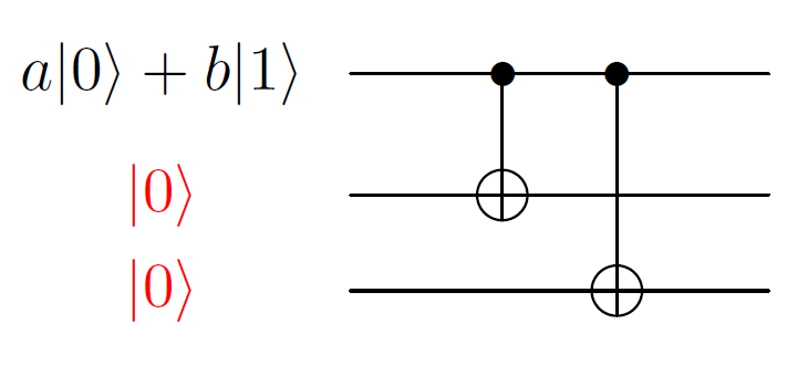
In Fig. 2.5, the single qubit information to be protected from the bit-flip noise is given by , where and satisfy . The state after encoding is obtained as . The syndrome measurement unit extracting the syndrome bits for the bit-flip noise is shown in Fig. 2.6 below. This unit uses two ancilla qubits indicated in red, such that the first ancilla measures and the second ancilla qubit measures on the three-qubit encoded state.

We see from this example of the -qubit bit-flip code that the stabilizer formalism serves as a powerful tool in constructing quantum codes, detecting and correcting errors. We refer to [lidar, Chapters 2,6] for a complete overview of the stabilizer formalism.
2.3 Approximate QEC

A perfect QEC protocol demands that a quantum code get mapped to mutually orthogonal subspaces, as captured by the QEC conditions in Eq. 2.5, under the action of errors. In practice, such a constraint might be too stringent and one can expect a codespace to get mapped to overlapping subspaces under the action of errors, as shown in Fig. 2.7. The idea of approximate QEC owes its origins to a four-qubit code that was constructed to protect a single qubit of information against amplitude-damping noise [leung]. This code was shown to satisfy approximate QEC conditions, which were obtained as a perturbed form of the perfect QEC conditions described in Eq. (2.4). As we discuss below, such an approximate quantum code with just four qubits performs comparable to the perfect -qubit code, in terms of the fidelity function.
Formally, a quantum code is said to be an approximate code for the noise channel , if there exists a recovery map such that is close, in terms of some well defined distance measure, to the initial state . The four-qubit approximate code, denoted as is obtained as the span of [leung],
| (2.9) |
where and are the logical qubits encoding a single qubit of information. The encoding circuit for the code can be obtained as shown in Fig. 2.8 below.

It is easy to verify that the code satisfies the perfect QEC conditions in Eq. 2.4 upto a deviation of , for amplitude-damping noise acting on each of the four qubits in an identical and independent manner. This four-qubit channel is represented as , where is the single-qubit amplitude-damping noise described in Eq. 5.2. Note that the representation of the four-qubit code, does not have a distance parameter, since the notion of distance is not well defined for an approximate code.
The code maybe considered the first known example of a channel-adapted code, since it is designed to correct specifically for amplitude-damping noise, rather than to correct for generic Pauli errors. Furthermore, it is also an approximate code since it satisfies a perturbed form of the Knill-Laflamme condition. Subsequently, there was a lot of interest in constructing channel-adapted codes as well as channel-adapted recovery schemes. A generalization of the approximate code for the amplitude-damping channel, based on stabilizer formalism was soon developed in Ref. [fletcher_codes]. A channel-adapted recovery map that corrects for the four-qubit code given in Eq. 5.2.1 affected by the amplitude-damping channel, was also constructed via a convex-optimization procedure [fletcher_rec]. A few other works in the past [kosut, yamamoto, reimpell] adopted similar numerical optimization strategies to look for channel-adapted codes or channel-adapted recoveries, or both, using the average entanglement fidelity as the figure of merit. Some of the past works also focussed on developing the approximate QEC (AQEC) conditions from an information-theoretic perspective [beny, beny2009, klesse, schumacher].
On the analytical front, a near-optimal map for reversing the dynamics was identified, using average entanglement fidelity as the figure of merit in [Barnum]. More recently, simple algebraic AQEC conditions were established in terms of the worst-case fidelity, based on the construction of a universal, recovery map, which was shown to be near-optimal for any encoding [hui_prabha]. This approach forms the basis of the methodology used in this thesis to construct and characterise approximate codes. In the following sections, we outline this algebraic approach to approximate QEC as well as the recovery map presented in Ref. [hui_prabha] in some detail, since we make use of these in subsequent chapters.
2.3.1 Petz Recovery map
We now define and discuss the universal near-optimal recovery map [hui_prabha], often referred to as the Petz map in the literature. For a given quantum channel with Kraus operators and a code with projector , the Petz map is defined as,
| (2.10) |
with Kraus operators . Noe that the inverse of is taken on its support. The recovery can be seen as the composition of three CP maps, , where is the projection onto the codespace, describes the adjoint of the noise channel with the Kraus operators , and is a normalization map given by, . The normalization map ensures that the map is trace-preserving (TP).
The recovery map in Eq. 3.4 was originally introduced in the work of Petz in an information-theoretic context [Petz], and is hence known in the literature as the Petz map. This map was shown to saturate Ulhmann’s theorem on the monotonicity of relative entropy [petz_entropy]. The structure of the Petz map is independent of the choice of the noise channel , it satisfies the TP condition below.
| (2.11) |
where is the projector onto the support of . We note that the map is unital for any noise channel , satisfying .
2.3.2 The worst-case fidelity function
The performance of a QEC protocol can be studied using the fidelity function [nielsen, Chapter 9], which is a measure of distance between quantum states. The fidelity between any two quantum states and is defined as,
| (2.12) |
takes values between and . Observe that for , , and when and have orthogonal support, . For a pure state , and for where is a CPTP map, the fidelity in Eq. 2.12 is obtained as,
| (2.13) |
Specifically, the worst-case fidelity [nielsen, Chapter 9] is a useful figure of merit in quantifying the performance of a QEC protocol, since it assures that a certain minimum fidelity is achieved by all the states on a given Hilbert space. The worst-case fidelity for a given pair of encoding and recovery map , for a noise , is defined as,
| (2.14) |
Equivalently, it is also useful to describe the performance of a QEC scheme in terms of the fidelity-loss function, which is defined as
| (2.15) |
Note that the fidelity is a quantity that is jointly concave in its arguments, which means that for any probability distribution and density matrices , ,
| (2.16) |
Suppose = , and = , then
| (2.17) |
For any pure state , it thus follows that,
| (2.19) | |||||
Thus, the lower bound on fidelity is achieved by a pure state as illustrated in Eq. 2.19. Hence, it is enough to minimize the fidelity function over the state space of just pure states to obtain the worst-case fidelity.
2.3.3 AQEC conditions and near-optimality of the Petz map
We now state and explain the AQEC conditions based on the Petz map in Eq. 3.4. Although the Petz recovery may not achieve the largest worst-case fidelity for given channel and code , it was shown to perform close to optimal in [hui_prabha]. Specifically, this near-optimality is captured by the bounds [hui_prabha, Corollary 4]),
| (2.20) |
where and are the fidelity losses if we used the optimal and Petz recoveries, respectively, for a given encoding and noise . An interesting point to note is that the code dimension also appears in Eq. 2.20. Thus, for smaller values of , the Petz recovery map is a good approximation of the optimal map.
Based on the near-optimality of the Petz map, one can obtain conditions for approximate QEC, as shown in [hui_prabha, Theorem 6].
Theorem 2 (Conditions for AQEC).
Consider a noise channel with Kraus operators , acting on a codespace with projector , such that,
| (2.21) |
where the scalars are obtained as , being the dimension of the codespace , and are traceless matrices. Then, there exists a recovery map with fidelity loss given by,
| (2.22) |
such that, for any , the code achives a worst-case fidelity for the noise (a) if , and (b) only if , where = .
In the case of a perfect QEC code, the matrices in Eq. 2.21 vanish and the matrix of scalars given in Eq. 2.4, leading us back to the perfect QEC conditions in Eq. 2.4. This shows that the Petz map is indeed the optimal map for perfect quantum codes.
In contrast to a perfect code, an approximate code with a non-zero in Eq. 2.21, gets mapped to overlapping, and hence indistinguishable subspaces under the action of errors as illustrated in Fig. 2.7. Hence, recovering the information could be even more challenging and one cannot construct unitaries to recover as in the case of perfect QEC. A detailed treatment of this approximate QEC approach and Petz recovery that we outlined in this section above can be found in [hui_prabha, prabha_thesis].
2.3.4 Recent developments in AQEC
We conclude this chapter with a brief review of some of the recent developments in AQEC. We first note that the AQEC formalism elaborated in the sections above, based on the Petz recovery, has been extended to study the case of subsystem codes in [prabha_aqec]. The performance of AQEC schemes has been studied for the case of generalized amplitude-damping channel, using a recovery similar to the Knill-Laflamme perfect recovery, in [cafaro]. This scheme uses the entanglement fidelity to study the efficiency of the protocol.
More recently, the work due to [elizabeth] demonstrates how approximate codes arise naturally in translation-invariant many body systems. This work also draws connections between quantum chaotic systems with ETH (Eigenstate Thermalization Hypothesis) and approximate quantum codes. More generally, the interplay between continuous symmetries and approximate quantum codes has been analyzed in great detail, in [preskill_symmetry], which also demonstrated the construction of quantum codes covariant with respect to a general group.
The Petz map and its variants have provided a fertile area of study, leading to several interesting directions of work. The Petz construction has been used in [todd] to show how orbital angular momentum properties of the photons can be protected from decoherence caused by atmospheric turbulence. An explicit construction of the Petz map has been provided for the case of guassian channels in [wilde]. More recently, [petz_implementation] demonstrated a quantum algorithm to implement the Petz map using the quantum singular value transformation. This algorithm provides a procedure to perform the pretty-good measurement which is a special case of Petz recovery, allowing for near-optimal state discrimination.
Chapter 3 Constructing adaptive codes using the Cartan form
3.1 Introduction
Interest in building quantum computing devices has grown steadily, with rapid progress in the last few years thanks to the fresh injection of industry support. Current quantum computing devices, like the ones being built by IBM, Google, and Rigetti, comprise only a few (at best, tens of) qubits, and are quite noisy. We are right now in the “NISQ era" [preskill2018quantum], a term referring to the near-to-intermediate-term situation where physical devices are too noisy and too small to implement regular quantum error correction (QEC) and fault tolerance schemes to deal with the noise in the device. Hence, there is a strong need to find better QEC and fault tolerance schemes with lower resource overheads, essential for the eventual implementation of robust and scalable quantum computing devices. Generally, QEC [shor, steane, calderblank, gottesman, knill] (see also a recent review [terhal]) tries to store the information to be protected in a special part of the quantum state space with the property that errors due the noise can be identified and their effects removed through a recovery procedure.
Much of the existing work on QEC centers around codes capable of removing the effects of arbitrary errors on individual qubits, powerful enough to deal with general, even unknown, noise. The stabilizer codes [nielsen], including the well-known Steane code [steane] and Shor code [shor], fall in this category of codes which can correct for single-qubit errors.
One cannot find codes capable of correcting an arbitrary error on any single qubit unless one uses at least five physical qubits to encode a one qubit of information [laflamme]. However, when there is a reasonable level of characterization of the noise afflicting the qubits, channel-adapted codes [fletcherthesis]— codes tailor-made to deal with the specific noise channel encountered in the physical device— become of interest. Such codes can be expected, and are known (see, for example, the -qubit code for amplitude-damping noise discovered in Ref. [leung]), to be less demanding in resources.
The most general formulation of channel-adapted codes requires full knowledge of the noise. We make the following experimentally well-motivated assumption [tannu] about the structure of the noise. We assume that the noise takes a tensor-product structure and propose a numerical algorithm to find good codespaces— regions of the state space resilient to the noise— among states with a nonlocal structure, using a Cartan decomposition of the encoding operation.
The question of finding channel-adapted codes can be formulated as an optimization problem [yamam, reimpell, fletcher_codes, kosut, wang], one of finding the combination of code and recovery that optimizes a chosen figure of merit for the given noise channel. When the figure of merit is the average entanglement fidelity [schum], one only has a double optimization over encoding (of a given block length) and recovery. This problem is known to be tractable via convex optimization techniques [reimpell, fletcher_rec, kosut].
In our work, we focus on finding channel-adapted codes that minimize the worst-case fidelity for the storage of a single qubit of information. We argue that we can, in practice, reduce the original triple optimization to a single optimization by making use of the Petz recovery [Petz], shown to be near-optimal [hui_prabha] for any noise channel and choice of code. The use of the Petz recovery leads to an analytical expression for the worst-case fidelity for codes encoding a single logical qubit. Furthermore, a key aspect of this work is that we can reduce the difficulty of this remaining numerical optimization over all possible encodings by employing a Cartan decomposition of the encoding operation, motivated by the noise-locality–code-nonlocality dichotomy. We vary only over the nonlocal pieces of the decomposition, thereby reducing the dimension of the search space. Altogether, these steps give a fast and easy algorithm for finding good channel-adapted codes for the worst-case fidelity, the preferred figure of merit for quantum computing tasks.
3.2 The optimization problem
We begin by describing the various ingredients in our approach to the problem of finding channel-adapted codes for the worst-case fidelity measure. We explain how to reduce the problem to a single optimization, over the encoding operation.
3.2.1 Basic formulation
Consider a physical quantum information processing system of dimension , with Hilbert space . The noise acting on the system can be described by a quantum channel, i.e., a completely positive (CP) and trace-preserving (TP) linear map, denoted by . acts on , the set of linear operators on , . Its action can be written as , for a set of (non-unique) Kraus operators , a structure that assures the CP nature of the map. The Kraus operators further satisfy , for the TP property.
To protect the quantum information from damage by the noise, QEC proposes to store the information—assumed to be a -dimensional Hilbert space of states—in a ()-dimensional subspace of , the Hilbert space of the physical system. We refer to as the codespace. The encoding operation —a unitary operation, and hence invertible—is a one-to-one mapping of states from to , . The action of the noise on the encoded state, the output of , can then be regarded as . After the action of the noise, the QEC protocol applies a suitable recovery map , a CPTP map that restores the state into the codespace, and in the process removing (hopefully most of) the errors due to the noise. If we want, we can then decode the physical state back into the quantum informational state of by applying the decoding operation, .
Traditionally, the QEC protocol, specified by the pair for given and , is chosen to satisfy (at least approximately) what are known as the QEC conditions [knill, hui_prabha], for successful removal of the errors caused by the noise. Here, it is more straightforward to think directly in terms of an optimization problem. For that, we first quantify the performance of a code (or, equivalently, ) with recovery for the noise process by a measure that compares the output state of the QEC protocol to the input state . We then characterize the performance of a given pair for noise , using the worst-case fidelity which is the square of the quantity defined in Eq. 2.14, as shown below.
| (3.1) |
Recall from Sec. 2.3.2 that it is enough to minimize and by extension also, over pure states. This minimization over usually has to be done numerically unless one has special properties that simplify the problem (as we will see below). Alternatively, one can make use of the fidelity loss quantity defined as,
| (3.2) |
We can now state the basic formulation of the optimization problem for channel-adapted codes: For given noise , and the available dimension of the physical system, the best code is given by the solution to the following optimization over encoding operations and recovery maps .
| (3.3) | ||||
This is the triple optimization, over the encoding , the recovery , and the input state , mentioned in the introduction.
We note that, in principle, one could also add an optimization over the dimension of the physical state space used to encode . For the current situation of independent noise on the physical system, one expects better fidelity with a larger number of physical qubits, as this will gives better “de-localization" of the information. However, in the current NISQ era, the number of physical qubits available for encoding the information will largely come from practical constraints. We thus take to be fixed, and find the best for that given .
We first reduce this triple optimization problem to a double optimization over and , by choosing the Petz recovery . Recall from Sec. 2.3.1 that the Petz map is defined as [Petz, hui_prabha],
| (3.4) |
where constitute the Kraus operators of . Here, is the projector onto the codespace , and the inverse of is taken on its support. Having fixed the recovery, our optimization problem now reduces to a double optimization of the form,
| (3.5) |
We denote the fidelity loss for an encoding as ; the optimal encoding is then the one that attains .
3.2.2 Fidelity loss for qubit codes
In this work we search for codes which preserve a qubit worth information. It turns out that the optimization problem of Eq. (3.5) can be further simplified, since the worst-case fidelity for encoding , or equivalently, the fidelity loss function , has a simple form for the case of qubit codes (i.e., ) with the Petz recovery. Specifically, can be easily computed via eigenanalysis [hui_prabha]. We recall the steps here, for completeness.
We encode a qubit into a two-dimensional codespace . For an orthonomal basis on , the Pauli basis (orthogonal but not normalized) for operators on , denoted as , can be defined in the usual way as,
| (3.6) | ||||
| (3.7) |
Codestates can then be described using the Bloch representation,
| (3.8) |
where is a real -dimensional vector — the Bloch vector for — with Euclidean length , and .
Consider the channel constructed by composing the noise followed by the Petz recovery, , acting on the codespace. is the map that enforces the pre-condition that we start in the codespace. is both trace-preserving [] and unital [], and its action can be expressed in the Pauli operator basis defined above, as the following matrix.
| (3.9) |
Note that is a real matrix with real matrix entries , with denoting a matrix of the non-zero entries. The action of on an input state can then be expressed in terms of the action on the Bloch vector as . The fidelity loss (for a given encoding that defines the subspace) is then, by straightforward algebra,
| (3.10) |
where , and is the smallest eigenvalue of . Here, the superscript denotes the transpose operation.
3.2.3 A single numerical optimization
In this way, we have reduced the minimization needed to compute the worst-case fidelity in Eq. 3.5 to a simple diagonalization of a matrix and finding its smallest eigenvalue. Thus we have only a single optimization left to do, to find the best channel-adapted code, namely,
| (3.11) |
The optimization over the encoding has to be done numerically. We parameterize the search space as follows. Every codespace is specified by orthogonal pure states in , forming a basis for . Varying over the codespace can then be thought of as starting with a fixed basis with elements, and then applying a rotation of the basis, via a unitary operator acting on the full -dimensional Hilbert space of the physical system. Choosing different codespaces then corresponds to choosing different unitary operators . The search space is then the set of all -dimensional unitary operators, each element of which is specified by real parameters.
As noted above, has to be computed numerically for each . This means that we do not have a closed-form expression for the gradient of our objective function, so that standard optimization methods that require a formula for the gradient do not work. This is easily solved, however, by going to methods that estimate the gradient numerically via gradient-descent algorithms. A well-known approach, the one that we used here, is the Nelder-Mead search technique (also known as the downhill simplex method) [nelderpaper, NumericalRecipes], which has been explained in Sec. A.1 of Appendix A.
3.3 Simplifying the search: The Cartan decomposition
As stated earlier, the optimization over involves a -dimensional search. For -qubit physical systems, the typical experimental scenario, where , the search space dimension grows exponentially with . It would hence be useful to further reduce the complexity of the search by considering a restricted search over the set of encoding unitaries . For that, we recall our focus, as motivated in the introduction, on noise channels with a tensor-product structure over the qubits. This local structure in the noise suggests the use of codes with a nonlocal nature. To separate the nonlocal pieces of the unitary search space from the local pieces, we make use of the Cartan decomposition, as described in the following paragraphs.
Our search space, originally comprising elements of the unitary group for an -qubit code, can be restricted to elements of the special unitary group without loss of generality. We then use the Cartan decomposition originally proposed in [khaneja_glaser], whereby any -qubit unitary is realised as a product of single-qubit (local) and multi-qubit (nonlocal) unitaries. The specific paramterization we use is due to [cartan], where the standard Pauli basis is employed to decompose an arbitrary element of in terms of its local and nonlocal parts in an iterative fashion.
Cartan form of
Recall that the special unitary group — the group of complex matrices with determinant one — forms a real Lie group of dimension . Let denote the corresponding Lie algebra, the algebra of traceless anti-Hermitian complex matrices with the Lie bracket , that is, times the commutator.
The central idea behind the Cartan form is the fact that any element of can be represented, up to local unitaries, using elements of two Abelian subalgebras and () of . This was shown in [khaneja_glaser] via an iterative decomposition of the form , where is generated alternately from elements of and , while and belong to the subgroup of generated by a subalgebra orthogonal to and . The exact structure of the decomposition depends on the choice of an appropriate basis for that can be obtained recursively for .
For example, for , one can use twofold tensor products of the single-qubit Pauli operators () as basis elements for the Lie algebra . Using this basis to partition into orthogonal subspaces leads to an identification of the Abelian subalgebras and . This leads to the well known Cartan form for any [Zhang2003, Rezakhani2004],
| (3.12) |
where , and are local, single-qubit unitaries, and , and are scalar parameters characterizing the nonlocal operators.
Following this intuition from , it was shown that a basis comprising -fold tensor products of the single-qubit Pauli basis can be obtained for any by an iterative process [cartan], which partitions into Abelian subalgebras and . The Cartan decomposition of any -qubit unitary operator can then be obtained as follows.
Cartan decomposition [cartan]. Any , for can be decomposed as,
| (3.13) |
Here, are product operators from , and are unitary operators nonlocal on the entire -qubit space, with and . The decomposition can be applied recursively, to further decompose each operator in in the same form as in Eq. (3.13), for all .
As in the case, the Cartan decomposition for again separates out the local and nonlocal degrees of freedom in an iterative fashion. However, for , a second Cartan decomposition is required in order to identify the factors that are nonlocal on the entire -qubit space. This stems from the fact that a pair of nontrivial Abelian subalgebras maybe identified for any , and this leads to a two-step decomposition. First, using the generators of the subalgebra , we obtain the unitary , as well as , such that for any , . Further Cartan decompositions of and using the generators of gives the form , where the operators are no longer nonlocal on the entire -qubit space. Starting with the bases for identified above, [cartan] provides a simple recursive prescription to identify the bases for the subalgebras , for any .
To illustrate how the above prescription can be used to obtain a nice parameterization of the encoding unitaries for QEC, we explicitly write down the Cartan form for and . Any element of can be constructed using the formalism in Eq. 3.13 as,
| (3.14) | ||||
As stated above, , and each element in can be obtained similarly from Eq. 3.12. Recall that the standard description of any unitary in requires real parameters, whereas the recursive Cartan decomposition described in Eq. 3.14 requires a total of real parameters. However, the key advantage of using the Cartan parameterization is that the nonlocal factors of any unitary in are easily described in terms of real parameters, namely, the set of ten real parameters , along with the three real parameters for each of the four factors.
Similarly, we note that any element can be decomposed as,
| (3.15) |
where , , 2, 3, and 4. Such a decomposition requires a total of real parameters including the set which parameterizes the fully nonlocal factors.
We simplify our numerical search for optimal encodings by fixing the local components in the Cartan form and searching only over the nonlocal degrees of freedom. This greatly reduces the dimension of our search space and allows us to search much faster, compared to an unstructured search. This restriction only to nonlocal degrees of freedom, as we will see from our examples in Sec. 3.4, does not lead to substantial loss in fidelity. Furthermore, choosing the local unitaries in the decomposition appropriately allows us to construct encoding unitaries with simple structures that permit easy circuit implementations of the encoding procedure.
An example of such a structured encoding would be to set all the s in Eq. 3.13 to be the identity operator, thus reducing the form of the encoding unitary to . This implies the following form for the encoding unitary in the case of ,
| (3.16) |
where refers to some non-zero complex number. Such a structured encoding with only non-local Cartan factors is easy to implement using only single-qubit gates and the cnot gate, as explained in Appendix A, Sec. A.2.
3.4 Examples
We now demonstrate the efficacy of our numerical approach to finding good codes through some examples. We consider -qubit noise channels of the form , where is a single-qubit channel on the -th qubit. The first few examples are for the case where all the s are the same channel, corresponding to the common experimental situation where all the qubits see the same environment and hence undergo the same noise dynamics. We focus on three examples, namely, the amplitude-damping channel, the rotated amplitude-damping channel, and an arbitrary (randomly chosen, no special structure) single-qubit channel.
In each example, we use the form of the encoding unitary in Eq. 3.13 to perform both unstructured as well as structured search over the space of all encoding unitaries. In an unstructured search, we retain the general form of the encoding unitary in Eq. 3.13, using all parameters, local and nonlocal, in our search. For the structured search, we adopt two different approaches. In the case of a structured search with trivial local unitaries, we set all the local () unitaries in the Cartan decomposition in Eq. 3.13 equal to the identity, and search only over the nonlocal parameters in Eq. (3.13). For example, while searching over the -qubit space, we retain the nontrivial -qubit nonlocal pieces as well as the -qubit pieces, but set all the single-qubit unitaries to identity. Alternately, we also implement structured search with nontrivial local () unitaries, where the choice of the local unitaries in the Cartan decomposition is guided by the structure of the channel. This kind of structured search with nontrivial local unitaries will be particularly relevant for the example of the rotated amplitude-damping channel discussed in Sec. 3.4.2.
3.4.1 Amplitude-damping channel
Recall from Eq. 5.2 that the single-qubit amplitude-damping channel is described by a pair of Kraus operators in the computational basis , as,
| (3.17) |
where flips the state to the state, imitating a “decay" to the state; the deviation of from the identity ensures the trace-preserving nature of the channel. We perform the numerical search outlined in Sec. 3.3 and obtain optimal encodings for , when , for and . We compare the performance of the codes we find with the various known codes in Fig. 3.1. In particular, we compare with the approximate code [langshor], given by the span of the states,
| (3.18) |
and the approximate code [leung], which is the span of,
| (3.19) |
Fig. 3.1 shows that the numerically obtained codes via structured (with trivial local unitaries) and unstructured search outperform the known approximate codes of the same length described in Eq. (3.18) and Eq. (5.2.1) respectively. We observe that the performance of the -qubit optimal codes is even better than the standard code, as seen in Fig. 3.1(b). In both figures, we have also plotted the worst-case fidelity for a single unprotected qubit under the noise channel. The fidelity of the unencoded qubit falls off linearly with the noise parameter, thus demonstrating the advantage of using the -qubit codes found using our procedure.
The codewords for the optimal ,-qubit codes found in our search are presented in Appendix A, Sec. . We also provide the encoding circuit corresponding to the optimal, structured -qubit code, as an example of how the codes that emerge out of the structured search admit simple encoding circuits. Finally, we note that our numerical search procedure is indeed fast. The unstructured search for a specific value of damping parameter takes a few hundred seconds on a standard desktop computer, while each structured search takes only a few milliseconds on the same computer.
3.4.2 Rotated amplitude-damping channel
As our Cartan decomposition uses the Pauli basis, it is important to test if our numerical search is robust against noise not aligned along the axes used to define the Pauli basis. We therefore consider amplitude-damping channels where the damping is no longer in the basis. Specifically, we consider the single-qubit rotated amplitude-damping channel described by the Kraus operators,
| (3.20) |
where is a pair of orthonormal vectors on the Bloch sphere. Such a pair of vectors can be parameterized with respect to the basis using spherical coordinates,
| (3.21) |
with , . The values of thus determine the damping direction.
We present numerical search results for the amplitude-damping channel aligned along three different directions in Fig. 3.2. In all three examples, the structured search with nontrivial local unitaries was implemented by fixing the local unitaries as . For example, when the damping noise is aligned along the -direction on the Bloch sphere, the basis is the eigenbasis of the Pauli operator and the local unitaries are fixed to be the Hadamard gate, which rotates the basis to the basis.
Fig. 3.2(a) shows the performance of different codes when the damping is with respect to the eigenstates, whereas Figs. 3.2(b) and (c) present the results for choices of damping direction not aligned with one of the standard Pauli axes. In all three cases, we observe that the codes obtained using the unstructured search offer only slightly better fidelity than the codes obtained using the structured searches. Furthermore, the codes obtained using nontrivial local unitaries are often distinct from, and offer better fidelity compared to the codes obtained using trivial local unitaries in the search. Once again, our search procedure is efficient, with the structured and unstructured searches taking between tens to hundreds of seconds on a standard desktop computer. As in the earlier case, we have also compared the performance of the -qubit optimal codes with the fidelity of the single unprotected qubit.
3.4.3 Random local noise
As a third example of the usefulness of our numerical search procedure, we search for good codes for , where is a randomly chosen single-qubit channel. A random qubit channel is generated using a Haar-random unitary acting on the system qubit and a single-qubit ancilla initialized to the state ; the unitary acts jointly on the qubit and the ancilla, after which the ancilla is traced out, yielding a single-qubit channel. We then admix with the identity channel to give a family of qubit noise channels , for different , of the form,
| (3.22) |
parametrizes the noise strength: for small values of , describes weak noise, which is the practically relevant case.
Using our numerical search procedure we now obtain optimal -qubit codes for the class of random local noise channels described by Eq. (3.22) in the weak noise regime, . For each choice of random , and hence , we use our numerical AQEC approach to identify good -qubit codes for the 4-qubit channel .
Fig. 3.3 shows the fidelities obtained for the optimal codes for four random choices of . We compare the performance of the four-qubit codes obtained via structured and unstructured searches with the performance of the code, for each random channel. The recovery procedure used in each case is the corresponding Petz recovery.
In Fig. 3.3, we observe that the best -qubit codes — structured or unstructured — have fidelities linear in the noise strength , suggesting that the -qubit Hilbert space might not be sufficient to distinguish amongst the no-error case and the eight single-qubit errors arising from the weak noise . This issue is clearly resolved when we use the code and the corresponding Petz recovery, since the fidelity is now quadratic to leading order in . Finally, we note that the -qubit codes do yield a better worst-case fidelity than the single unencoded qubit under the action of the noise channel.
3.5 Conclusions
We have described a numerical search algorithm to find good quantum codes, using the worst-case fidelity as the figure of merit. By choosing the recovery map as the Petz recovery, we have reduced the general problem from a triple optimization over the encoding, recovery, and input states, to a single optimization over the encoding map only. Furthermore, the use of the Cartan decomposition, motivated by the typical scenario of independent per-qubit noise, allowed for a reduction of the search space to structured encodings, with performance comparable with the more expensive unstructured ones, as illustrated by our examples.
The ability to identify channel-adapted codes that involve fewer qubits than the stabilizer codes targeting arbitrary noise, might suggest that the corresponding encoding/decoding circuits might also be smaller in size. In fact, the well-known -qubit channel-adapted code due to Leung et al [leung] does have a much simpler encoding circuit [fletcherthesis] than the -qubit stabilizer code, and the encoding circuit is made up of only Clifford gates. Furthermore, in Chapter 4 we demonstrate the usefulness of our shorter-length optimal numerical codes using a specific application.
In our search for the quantum codes we have assumed that the encoding/decoding gates are perfect. This is of course the standard assumption in any discussion on QEC codes in the literature. However, the gates used to do the error correction are indeed the same ones as those used to do computation, so this assumption has to be relaxed, taking us into the domain of fault-tolerant quantum computing [gottesman_FT]. Our work deals with the first step of finding the optimal code for a given noise process. Extending this framework to fault tolerance is the next step for future work. In this context, our work provides an easy platform to explore and discover a large number of good candidate codes, which can then be individually examined to find the one that can be most easily implemented in a fault-tolerant manner. For the first time, we make an attempt to build a fault-tolerant computation scheme using the channel-adapted -qubit code [leung] in Chapter 5.
Chapter 4 Quantum State Transfer using Adaptive Quantum Codes
4.1 Introduction
Quantum communication entails transmission of an arbitrary quantum state from one spatial location to another. Spin chains are a natural medium for quantum state transfer over short distances, with the dynamics of the transfer being governed by the Hamiltonian describing the spin-spin interactions along the chains. Starting with the original proposal by Bose [bose] for state transfer via a -d Heisenberg chain, several protocols have been developed for perfect as well as pretty good quantum state transfer via spin chains.
Perfect state transfer protocols typically involve engineering the coupling strengths between the spins in such a way as to ensure perfect fidelity between the state of sender’s spin and that of the receiver’s spin [christandl, christandl2005perfect, albanesemirror, karbach, di]. Alternately, there have been proposals to use multiple spin chains in parallel, and apply appropriate encoding and decoding operations at the sender and receiver’s spins so as to transmit the state perfectly [conclusive, perfect, efficient]. Experimentally, perfect state transfer protocols have been implemented in various architectures including nuclear spins [bochkin] and photonic lattices using coupled waveguides [perez2013, chapman].
Relaxing the constraint of perfect state transfer, protocols for pretty good transfer aim to identify optimal schemes for transmitting information with high fidelity across permanently coupled spin chains [godsil2012, godsil]. One approach is for example to encode the information as a Gaussian wave packet in multiple spins at the sender’s end [osborne, hasel]. Moving away from ideal spin chains, quantum state transfer has also been studied over disordered chains, both with random couplings and as well as random external fields [perfect, ashhab, chiara].
Here, we study the problem of pretty good state transfer from a quantum channel point of view. It is known [bose] that state transfer over an ideal chain (also called the Heisenberg chain) can be realized as the action of an amplitude-damping channel [nielsen, Chapter 8] on the encoded state. Naturally, this leads to the question of whether quantum error correction (QEC) can improve the fidelity of quantum state transfer. Such an improvement has been reported by making use of the -qubit code for pretty good transfer over the Heisenberg spin chain [allcock]. On a related note, QEC-based protocols have also been developed for pretty good state transfer over noisy [kay, kay2018perfect] chains.
In our work we study the role of adaptive QEC in achieving pretty good transfer over a class of -d spin systems which preserve the total spin. This includes both the as well as the Heisenberg chains, and more generally, the chain. We use an approximate QEC (AQEC) code, which has been shown to achieve the same level of fidelity as perfect QEC codes for certain noise channels while making use of fewer physical resources [leung, fletcher_codes, hui_prabha, cafaro]. Our protocol involves the use of multiple identical spin chains in parallel, with the information encoded in an entangled state across the chains. This is in contrast to the protocols in [kay, kay2018perfect] which use perfect QEC codes and encode into multiple spins on a single chain. Using the worst-case fidelity between the states of the sender and receiver’s spins as the figure of merit, we demonstrate that pretty good state transfer maybe achieved over a class of spin-preserving Hamiltonians using an approximate code and a channel-adapted recovery map.
We present analytical and numerical results for the fidelity of state transfer obtained using our QEC scheme, for ideal as well as disordered chains. The presence of disorder in a -d spin chain is known to lead to the phenomenon of localization [anderson]. Here, we analyze the distribution of the transition amplitude for a disordered chain, with random coupling strengths which are drawn from a uniform distribution. We modify the QEC protocol suitably so as to ensure pretty good transfer when the disorder strength is small. As the disorder strength increases, our analysis points to a threshold beyond which QEC does not help in improving the fidelity of state transfer.
4.2 Preliminaries
We consider a general -d spin chain with nearest neighbour interactions described by the Hamiltonian,
| (4.1) | |||||
where, and are site-dependent exchange couplings of a ferromagnetic spin chain, denote the magnetic field strengths at each site, and, are the Pauli operators at the site. The spin sites are numbered as . We assume that the sender’s site is the spin and receiver’s site is the spin.
We denote the ground state of the spin as . Since we are interested in transmitting a qubit worth of information along the chain, we will work within the subspace spanned by the set of single particle excited states , with denoting the state with the spin alone flipped to . The Hamiltonian in Eq. (4.1) preserves the total number of excitations, that is, and hence the resulting dynamics is restricted to the -dimensional subspace spanned by the single particle excited states and the ground state.
The sender encodes an arbitrary quantum state at the site, with the coefficients and parameterized using a pair of angles as , . The initial state of the spin chain is thus given by,
| (4.2) |
where is the state of the spin chain with only the spin is flipped to and all other spins set to . Under the action of the Hamiltonian described in Eq. (4.1), after time , the spin chain evolves to the state (here, and in what follows, we set ),
Following [bose], the state of the receiver’s spin at the site after time , denoted as , is obtained by tracing out all the other spins from the state of the full spin chain , as follows.
| (4.3) | |||||
where,
| (4.4) |
is the transition amplitude, which gives the probability amplitude for the excitation to transition from the site to site. The function satisfies,
| (4.5) |
where is the delta function with for and for .
As in the case of the Heisenberg chain [bose], we obtain the reduced state in Eq. (4.3) at receiver’s end as the action of a quantum channel on the input state. Specifically,
| (4.6) |
where and are the Kraus operators that describe the action of the channel. It is easy to see that the operators have the following form when written in the basis.
| (4.7) |
The Kraus operators in Eq.(4.7) lead to a channel that has the same structure as the amplitude-damping channel described in Eq. 5.2, but is more general since the parameter characterizing the noise in the channel is complex.
The standard amplitude-damping channel (Eq. 5.2) parameterized by a real noise parameter , is the quantum channel induced in the original state transfer protocol in [bose], where the Hamiltonian considered is a Heisenberg chain in the presence of an external field of the form ,
| (4.8) |
By choosing the intensity of the -field appropriately, it is possible to adjust the phase of the complex amplitude to be a multiple of and hence replace by , thus obtaining the amplitude-damping channel described in Eq. (5.2).
While much of the past work on state transfer has focused on the Heisenberg Hamiltonian in Eq. (4.8), here, we will focus on the more general Hamiltonian in Eq. (4.1). We study the problem of transmitting an arbitrary quantum state from the site to the site of an -spin chain. We quantify the performance of the protocol in terms of the fidelity between the final state and the input state . Specifically, we use the square of the worst-case fidelity defined in Eq. 2.14,
where the minimization is over all possible input states . We say that pretty good state transfer is achieved when the worst-case fidelity , for some .
Let and refer to the amplitude and phase respectively, of the noise parameter of the general quantum channel in Eq. (4.7). For such a channel, the worst-case fidelity depends on both the amplitude as well as the phase . However, following the original protocol in [bose], if we choose the magnetic fields so as to ensure that is a multiple of , we can show that,
| (4.9) |
In what follows, we examine how the worst-case fidelity may be improved using techniques from quantum error correction. In particular, by obtaining a functional relationship between the worst-case fidelity and the transition amplitude using an adaptive QEC procedure, we show how the fidelity can be improved by an order of the magnitude in the noise parameter.
4.3 State Transfer protocol based on adaptive QEC
Given a specific form of the spin-conserving Hamiltonian in Eq. (4.1), it is possible to estimate and for a specific choice of sites and by making repeated measurements on the spin chain [perfect]. Knowing , we may apply a phase gate of the form,
| (4.10) |
to change the encoding basis to . In this rotated basis, the channel in Eq. (4.7) is identical to the amplitude-damping channel described in Eq. (5.2). At the level of the Hamiltonian, this is the same as choosing the field strengths so as to make the phase trivial. Indeed, by making an appropriate choice of magnetic fields, it is always possible to transfom the spin-preserving Hamiltonian in Eq. (4.1) into an interaction as in Eq. (4.8) (see [kayreview]) and hence map the underlying noise channel to an amplitude-damping channel.
One naïve approach to improving the fidelity of state transfer is to therefore first apply the -gate and then use any of the well known QEC protocols which correct for amplitude-damping noise [leung, hui_prabha, fletcher_codes, AD_reliable2017]. However, such an approach fails in the presence of disorder. When we consider a disordered -d spin chain wherein either the couplings or the fields in Eq. (4.1) maybe random, the underlying noise channel is stochastic. The two real parameters and characterizing the noise in the channel vary with each disorder realization, and hence an encoding procedure that relies on knowledge of a specific realization of is not useful. Moreover, implementing a phase gate as in Eq. (4.10) based on the disorder-averaged value of does not help – such a phase gate will no longer cancel out the arbitrary (random) phase in Eq. (4.7) and we do not obtain an amplitude-damping channel in the rotated basis after the action of the phase gate.
We would therefore like to tackle the problem of correcting for the more general noise channel in Eq. (4.7). Taking inspiration from the structural similarity to the amplitude-damping channel, we propose a QEC protocol using an approximate -qubit code [leung] along with the channel-adapted near-optimal recovery proposed in [hui_prabha]. The code has already been described in Eq. 5.2.1. We recall here that the -qubit codespace is realised as the span of the following pair of orthogonal states,
| (4.11) |
This code was shown to be approximately correctable for amplitude-damping noise, both in terms of worst-case fidelity [leung] as well as entanglement fidelity [cafaro]. The code is approximate in the sense it does not satisfy the conditions for perfect quantum error correction [nielsen], for any single-qubit error.
We now use the Petz recovery mentioned in Sec. 2.3.1 (Chapter 2), known to achieve better worst-case fidelity for the case of amplitude-damping channel and -qubit code compared to the standard QEC procedure [hui_prabha]. Recall from Sec. 2.3.1 that the Petz map can be described in terms of the Kraus operators of the noise and the projector onto the codespace, as follows,
| (4.12) |
where the inverse of is taken on its support.

The quantum state transfer protocol with QEC is implemented using a set of unmodulated, identical, spin chains. Fig. 4.1 depicts a schematic of our protocol. The initial, encoded state is now an entangled state across the four chains, involving only a single spin (the site)in each of the chains.
| (4.13) |
Once the initial state is prepared, the four chains are allowed to evolve in an uncoupled fashion, according to the Hamiltonian in Eq. (4.1). After time , the state at the receiver’s site is a joint state of the site of the four chains, and is described by action of the map with the time-dependent noise parameter . Thus,
where are the Kraus operators of the -qubit noise channel realized as four-fold tensor products of the operators and in Eq. (4.7). After evolving the chains for time , the recovery map is applied at the receiver’s site of the four spin chains. The final state at the receiver’s end after the QEC protocol is obtained as,
with the Kraus operators given by,
| (4.14) |
As usual, is the projector onto the -qubit space described in Eq. (4.3). The fidelity of the -chain quantum state transfer protocol is then given by,
where the minimization is over all states in the codespace . As before, pretty good transfer is achieved when the worst-case fidelity is high, that is, , for . We now present a bound on the fidelity of state transfer using our adaptive QEC protocol, in terms of the transition amplitude .
Theorem 3.
The fidelity of quantum state transfer from site to site under a spin-conserving Hamiltonian as in Eq. (4.1), using the -qubit code and adaptive recovery at time , is given by,
| (4.15) |
where .
Proof.
We first rewrite the Kraus operators given in Eq. (4.7), as,
where, and are the absolute value and phase of the complex-valued transition amplitude . The state after the -qubit recovery map is then given by,
The composite map comprising noise and recovery has Kraus operators of the form,
| (4.16) |
The key step in obtaining the desired fidelity is to show that the Kraus operators of the composite map written above are independent of . First, we write out in the (standard) computational basis of the -qubit space.
where are polynomial functions of the transition amplitude . The -dependence in this pseudo-inverse operator occurs only in the span of . Since is sandwiched between the Kraus operators of the -qubit channel and their adjoints, we also write down the Kraus operators in the computational basis. Then, an explicit computation reveals that the -dependence gets conjugated out for each of the Kraus operators in Eq. (4.16). We refer to Appendix for the details of this calculation. Furthermore, we also prove a general theorem that states that is independent of for any choice of the in Appendix .
Hence the final state after noise and recovery can be expressed as a linear sum of terms that are independent of . Since the parameter is effectively suppressed, the fidelity after using -qubit code and the universal recovery in Eq. (4.7), is purely a function of .
The fidelity corresponding to the initial state can thus be obtained as,
| (4.17) | |||||
where refers to terms of order and higher. Parameterizing and as , , the fidelity attains its minimum value at (), so that the worst-case fidelity over the -qubit code is given by,
∎
Our result shows that using the adaptive recovery in conjunction with the approximate code leads to a fidelity that is independent of the phase of the complex noise parameter . Thus, to optimize the fidelity of state transfer between the and site of a chain of spins evolving according to the Hamiltonian in Eq. (4.1), we simply need to find the time at which is maximized. Recall that the worst-case fidelity without QEC (using the single chain protocol) is linear in the parameter , as observed in Eq. (4.9). Thus we see an improvement in fidelity with QEC, as expected.
Furthermore, our estimate of the worst-case fidelity implies that so long as the noise strength is such that , the adaptive QEC protocol achieves better fidelity than the single chain protocol without QEC. This constraints the noise strength to satisfy . This in turn implies a threshold for the transition amplitude, namely, , below which our adaptive QEC protocol will not offer any improvement in the fidelity of state transfer.
4.4 Results for the -d Heisenberg Chain
As a simple example to illustrate the performance of the adaptive QEC protocol, we now consider a special case of the Hamiltonian in Eq. (4.1), namely, an -length, ideal Heisenberg chain, with and , for all . This is also often referred to as the -chain in the literature. Setting without loss of generality, we present numerical results on the fidelity of state transfer from the first () to the () site.

Fig. 4.2 compares the performance of state transfer protocols with and without QEC. In particular, it compares the performance of our -chain state transfer protocol using the -qubit code in [leung] as well as a -qubit code given in Appendix , obtained via our numerical search procedure described in Chapter 3, with the single-chain (no QEC) protocol [bose] and the -chain protocol proposed in [allcock]. For each , we plot the fidelity of state transfer from the site to the site on a -length spin chain, after a time chosen such that is maximum at , for .
From the plot we see that the QEC-based protocols achieve pretty good state transfer over longer distances than the single chain protocol. Furthermore, using approximate QEC it is possible to achieve as high as fidelity as with the standard -qubit code, using fewer spin chains. Specifically, in the regime of small noise parameter , it is easy to compute that the worst-case fidelity obtained using the -qubit code is,
| (4.18) |
Correspondingly, a -chain protocol performs better than the single chain protocol when , implying that the transition amplitude should satisfy , which is a higher threshold than that required by our adaptive QEC protocol.
For the ideal Heisenberg chain, it was recently shown that [godsil], there always exists a time at which if and only if the length of the chain is a power of , that is, . In other words, pretty good state transfer is always possible between the ends of a Heisenberg spin chain whose length is of the form . We may therefore consider improving the performance of our QEC-based protocol by repeating the error correction procedure every sites. Specifically, we can achieve pretty good state transfer over a chain of arbitrary length , by stitching together smaller chains whose lengths are of the form . At every stage of the repeated QEC protocol, there are exactly interacting spins and the rest of the spin-spin-interactions are turned off.
Fig. 4.3 shows an example of the resulting improvement in fidelity when the QEC protocol is repeated every sites. For comparison, we plot the worst-case fidelity obtained by stitching together a sequence of length- chains, without QEC. The repeated QEC protocol proceeds as follows. We first implement our QEC protocol for an -spin chain, evolving for time at which maximizes. We repeat this procedure some times, where is the largest integer such that and finally perform QEC for the remaining sites for the same waiting time . Such a repeated QEC protocol indeed enables pretty good transfer for much longer lengths, as seen in the plot.
More generally, if is the fidelity of the single-shot QEC protocol, repeating the procedure times gives us a fidelity of , with,
where is the noise parameter obtained after repeating QEC times.
4.5 Quantum state transfer over a disordered Heisenberg chain
Moving away from an ideal spin chain with a fixed, uniform coupling between successive spins, we now study state transfer over a disordered chain, where the spin-spin couplings are randomly drawn from some distribution. It is well known that the presence of disorder in a -d spin chain leads to the phenomenon of localization [anderson] of information close to one end of the chain. It is therefore a challenging task to identify protocols which achieve perfect or pretty good transfer over disordered spin chains, overcoming the effects of localization.
Past work on disordered chains has primarily focused on the chain. Starting with a modulated chain that admits perfect state transfer, both random magnetic field and random couplings have been studied [chiara]. Alternately, an unmodulated chain with random couplings at all except the sender and receiver sites has also been studied [ashhab].
When viewed in the quantum channel picture, the presence of disorder becomes an additional source of noise. The role of QEC in overcoming the effects of disorder has been studied both for the [kay] as well as the Heisenberg chains [allcock]. The QEC protocol for a noisy chain with random couplings involves encoding into multiple spins on a single chain using modified CSS codes [kay]. The QEC protocol in [allcock] encodes into multiple identical, uncoupled chains using the standard -qubit code, while also requiring access to multiple spins at the sender and receiver ends of each of the chains. Furthermore, the protocol based on the -qubit code involves choosing an encoding based on the phase of the transition amplitude (as explained in Sec. 4.3), which in turn is specific to the disorder realization. This makes the QEC procedure hard to implement in a practical sense.
Here, we show how the channel-adapted QEC procedure described in Sec. 4.3 can be used to achieve pretty good state transfer over an chain with random couplings. As before, we quantify the performance of the state transfer protocol in terms of the fidelity between the initial and final states. When the underlying quantum channel is stochastic, as in the case of a disordered chain, we use the disorder-averaged worst-case fidelity , to characterize the performance of the state transfer protocol. We say that pretty good state transfer is achieved by a certain choice of code and recovery when the corresponding disorder-averaged fidelity , for some .
We consider a disordered Heisenberg chain with couplings = , where are independent, identically distributed random variables drawn from a uniform distribution between and is the mean value of the coupling strength, which we may set to , without loss of generality. Note that such a Hamiltonian conserves the total spin and hence falls within the universality class discussed in Sec. 5.2.
Consider a state transfer protocol, where the sender wishes to transmit the state from the site to the site via the natural dynamics of the chain. As before, the final state at the receiver’s site, tracing out the other spins can be realized as the action of a quantum channel ,
with the same Kraus operators as in Eq. (4.7). The key difference however is in the nature of the noise parameter : in the case of the disordered chain, the transition amplitude between site and for a chain of length allowed to evolve for a time , is a random variable whose value depends on the specific realization of the disorder variables . The distribution of for given set of values depends on the distribution over which the disorder variables are sampled. To illustrate our point, we specifically consider below the case where the coupling strengths are independently sampled from a uniform distribution.
4.5.1 Transition amplitude in the presence of disorder
The Heisenberg Hamiltonian with static disorder in the coupling strengths, has the form,
| (4.19) |
Here, the effect of disorder is introduced via the i.i.d. random variables which take values over a uniform distribution between . The quantity is called the disorder strength, and is the mean value of the coupling coefficient. We may view the disordered Hamiltonian as a sum of the form , where denotes the ideal Hamiltonian studied in the previous section and is given by,
captures the effect of disorder in the spin chain and can be treated as a perturbation of the Hamiltonian . Since , the transition amplitude maybe evaluated using the so-called time-ordered expansion, also referred to as the Dyson-series [dyson].
Specifically, the transition amplitude between the and site for the disordered Hamiltonian in Eq. (4.19) is given by (setting ),
where is the time-ordering operator which has been expanded to first order in the perturbation in the final equation. As before, denotes the transition amplitude between the and sites in the case of an ideal chain of length , without disorder.
Thus, using the time-ordered expansion, the transition amplitude in the presence of disorder can be evaluated as a perturbation around the zero-disorder value , of the form,
| (4.20) |
The explicit forms of the complex coefficients are given in Eq. () in Appendix . A similar approach was used in [chiara] to study deviations from perfect state transfer due to the presence of disorder in an chain.
Using the form of the transition amplitude stated in Eq. (4.20), we obtain the distribution of real part of the transition amplitude , up to first order in the perturbation , as,
| (4.21) |
where and the function is defined as
The functions are linear combinations of the form,
| (4.22) |
where and denote the real part of the coefficients in Eq. 4.20. Since there are such coefficients for a spin chain of length , the sum over ranges from to . There are distinct linear combinations of the form , corresponding to the distinct -bit binary strings parameterized by , so that the sum over runs from to . The form of the distribution is identical for the imaginary part , with the real parts of and replaced by their imaginary parts. We refer to Eqs. (), () in Appendix for a detailed description of the distributions of the real and imaginary parts of the disordered transition amplitude.
The key salient feature we observe from calculating the distribution functions above is that the limiting distribution in the case of no disorder (), is indeed a delta distribution peaked around . Furthermore, in Appendix we also explicitly evaluate the mean and variance of and show that the mean is equal to the zero-disorder value of , up to (see Eq. ). The variance goes as , as shown in Eq. (), making it vanishingly small in the limit of small . This observation leads us to propose a modified QEC protocol for state transfer over disordered chains, using an adaptive recovery based on the disorder-averaged transition amplitude .
The analysis presented thus far holds for any pair of sites on a spin chain of length . As an example, we consider the specific case of an -length chain, with and . We plot the distribution of the real part of the transition amplitude at some fixed time , for disorder strengths and , in Figs. 4.4 and 4.5 respectively. We see that when the disorder strength is small enough, the transition amplitude is indeed distributed like a delta function peaked around the zero-disorder value. For large values of , the distribution spreads out quite a bit and its mean also shifts closer to zero, giving rise to a very small transition amplitude. The corresponding figures for are presented in Appendix .
4.5.2 Adaptive QEC for a -d disordered chain
To summarize, the quantum channel for state transfer in the presence of disorder has the same structure as that of the ideal chain, but with a stochastic noise parameter , since the transition amplitude is now a random variable whose value depends on the random couplings . However, as discussed in Sec. 4.5.1, for small enough disorder strengths, is peaked sharply around its mean value, and we may consider the disorder-averaged amplitude as a good estimate of the noise.
We therefore propose an adaptive QEC procedure for a disordered chain involving the -qubit code in Eq. (4.3) and a recovery map with the same structure as that used in the case of the ideal chain, described in Eq. (4.14). However, unlike the ideal case, the value of the channel parameter used in the recovery is different from the one in actual noise channel : the recovery map uses the disorder-averaged amplitude , and is therefore independent of the specific disorder realization, whereas the noise channel has the parameter which changes with every realization.
To illustrate the performance of this modified recovery map, we present numerical results for quantum state transfer from the first site () to the site ()on an -spin chain. Fig. 4.6 shows the disorder-averaged worst-case fidelity obtained using the -qubit code and the adaptive recovery , for an -spin chain. For disorder strengths , our adaptive QEC protocol achieves pretty good transfer, with fidelity-loss . Beyond , we notice that since the effects of localization are too strong to be counteracted by QEC.
This is further borne out by our detailed analysis of the distribution of the transition amplitude in the presence of disorder (see Appendix ). In particular, our expressions for the mean and standard deviation of the transition amplitude indicate that until , the disorder-averaged value is close to the value of the transition amplitude in the ideal (zero-disorder) case, and the standard deviation is insignificant compared to the mean. However, as the disorder strength increases further, the disorder-averaged value starts dropping and the standard deviation becomes comparable to the average value. Thus the effective noise parameter of the underlying quantum channel becomes too strong for the QEC procedure to be effective.
The fact that is a threshold of sorts can be seen more directly by studying the variation of the disorder-averaged transition amplitude with disorder strength. Previous studies on localization in disordered chains have used such a quantity, namely , as an indicator of the extent of localization [ashhab, chiara].
In Fig. 4.7, we plot the disorder-averaged transition amplitude for a fixed time and different disorder strengths , as a function of the receiver site , for the Heisenberg chain in Eq. (4.19). Empirically, we see that this plot follows an exponential distribution. The curves take the form , where are functions of disorder strength and is the localization length, i.e. the length at which falls to of its maximum value. This would mean that in Fig. 4.7 for each site , the disorder averaged transition probability gets suppressed exponentially depending on the strength of the disorder . Therefore, with increase in disorder strength , the localization effects become more pronounced.
Specifically, when the disorder strength crosses , the square of the transition amplitude between the ends of the -spin chain falls below on average. However, we know from the fidelity estimate in Theorem 3 that the adaptive QEC protocol improves fidelity if only if . Thus, for end to end state transfer on an -length disordered Heisenberg chain, is indeed a threshold beyond which the adaptive QEC protocol cannot help in improving fidelity. Since our analysis of the distribution of the transition amplitude presented in Sec. 4.5.1 as well as the fidelity expression in Theorem 3 hold for any we can always identify such a threshold for a specific set of values.
4.6 Conclusions
We develop a pretty good state transfer protocol based on adaptive quantum error correction (QEC), for a universal class of Hamiltonians which preserve the total spin excitations on a linear spin chain. Based on the structure of the underlying quantum channel, we choose an approximate code and near-optimal, adaptive recovery map, to solve for the fidelity of state transfer explicitly. For the specific case of the ideal Heisenberg chain, our protocol performs as efficiently as perfect-QEC-based protocols. Using repeated QEC on the chain, we are able to achieve high enough fidelity over longer distances for an ideal spin chain.
In the case of disordered spin chains the underlying quantum channel is stochastic. For the case of a disordered -d Heisenberg chain, we study the distribution of the transition amplitude, which in turn is directly related to the stochastic noise parameter of the noise channel. By suitably adapting the recovery procedure, we demonstrate pretty good transfer on average, for low disorder strengths.
It is an interesting question as to whether such channel-adapted QEC techniques maybe used to achieve pretty good state transfer for other universal classes, such as the transverse-field Ising model and the -chain. It is also an open problem to obtain an efficient circuit implementation of the adaptive recovery map discussed here.
Chapter 5 Achieving fault tolerance against amplitude-damping noise
Achieving fault tolerance against amplitude damping noise
5.1 Introduction
A practical quantum computer is prone to noise, both due to the fragile nature of quantum states but also due to imperfect gate operations. This necessitates the theory of quantum fault tolerance, which shows that reliable and scaleable quantum computing is possible even with a noisy quantum memory and noisy quatum gates, provided the noise rates are below a certain threshold [nielsen, gottesman97]. A fault-tolerant quantum computation proceeds by first encoding the physical qubits into a quantum error correcting (QEC) code. Subsequently, encoded gate operations are performed on the encoded qubits in a way that does not let the errors spread catastrophically. Errors are removed from the system via periodic syndrome checks performed on ancillary qubits, before they accumulate to a point where the damage becomes irreparable. The fundmental basis for any quantum fault tolerance scheme is the threshold theorem, which states that scalable quantum computation is possible provided the physical error rate per gate or per time step is below a certain critical value called the threshold [gottesman_FT].
Starting with Shor’s original proposal [shor_ft], the early works on quantum fault tolerance focussed on developing fault-tolerant schemes using general pupose QEC codes, specifically CSS codes such as polynomial codes [aharonov] and the Steane code [preskill_FT]. Subsequently, fault tolerance thresholds have been estimated incorporating concatenation [steane, aliferis], magic-state distillation [magic_2005], as well as teleportation-based schemes [knill_FT]. Typical threshold estimates of the allowed error rates range between and , as seen from Table 1.1, which contains a summary of various fault tolerance schemes and the threshold values achieved for specific noise models. More recently, surface codes have emerged as a very promising candiate for achieving fault-tolerance [raus_FT] with threshold estimates ranging between , although the resource overhead requirements are often as high as - physical qubits per logical qubit. We refer to [terhal] for a recent overview of fault-tolerant schemes using surface codes and colour codes in different dimensions.
The fault tolerance threshold obtained for a given QEC code or a class of codes depends crucially on the error model under consideration [knill_nature]. Most of the threshold estimates obtained so far have assumed either symmetric depolarizing noise or erasure noise. However, when the structure of the noise associated with a given qubit architecture is already known, a fault tolerance scheme tailored to the specific noise process could be advantageous, both in terms of less resource requirements as also in improving the threshold. This is borne out by the fault tolerance prescription developed for biased noise, in systems where the dephasing noise is known to be dominant [aliferis_biased, FT_assymetry]. This prescription was used to obtain a universal scheme for pulsed operations on flux qubits [aliferis_biasedExp], taking advantage of the high degree of dephasing noise in the cphase gate, leading to a numerical threshold estimate of for the error rate per gate operation.
Motivated by this example, we address the question of whether it is possible to develop fault tolerance schemes for channel-adapted codes [hui_prabha]. QEC codes adapted to specific noise models are often known to offer a similar level of protection as the general purpose codes, while using fewer qubits to encode the information [leung, fletcherthesis]. Furthermore, in today’s era of noisy intermediate-scale quantum (NISQ) devices [preskill_nisq], there has been growing interest in identifying shorter QEC codes that are amenable to fault-tolerant circuit constructions. For example, it has been demonstrated [gottesman_2016, flammia] that a family of fault-tolerant encoding and error-detection circuits can be constructed using five qubits for the erasure code, using which a criterion to test experimental fault tolerance may also be derived.
In our work [ak_ft], we develop fault-tolerant gadgets for qubits that are susceptible to amplitude-damping noise. Physically, this corresponds to a relaxation process and is known to be a dominant source of noise in superconducting qubit systems, for example. Moving away from general purpose codes, we use the well known -qubit code [leung] to develop gadgets that are fault-tolerant against local, stochastic, amplitude-damping noise. We analytically estimate the error threshold for the logical cphase, as well as the memory threshold, using our prescription. Our work thus provides the first rigorous level- threshold estimates for fault tolerance against amplitude-damping noise. Given the approximate nature of the code used here, it is not immediately clear as to how our our level- gadgets maybe concatenated to obtain fault tolerance at higher levels.
5.2 Preliminaries
We follow the basic framework of quantum fault tolerance developed by Aliferis et al. [aliferis], which we briefly review this formalism here for completeness. In a fault-tolerant quantum computation, ideal operations are simulated by performing encoded operations on logical qubits. Encoded operations, in turn, are implemented by composite objects called gadgets which are made of elementary physical operations such as single- and two-qubit gates (including identity gates for wait times), state preparation, and measurements. A location refers to any one of these elementary physical operations. A location in a gadget is said to be faulty whenever it deviates from the ideal operation, and can result in errors in the qubits storing the computational data. The key challenge of is to design the gadgets in such a way as to minimize the propagation of errors due to the faults within the same encoded block.
In what follows we refer to the elementary physical operations are called unencoded gadgets. Our goal is to construct the encoded or logical gadgets corresponding to the -qubit code, which are resilient to a specific local stochastic noise model, namely, the amplitude-damping channel defined in Eq. 5.2 below. In our scheme, we use the following unencoded operations to build the fault-tolerant encoded gadgets.
| (5.1) |
Here, and refer to the eigenstates of single-qubit and Pauli operators respectively, and refer to measurements in the and basis respectively. cnot refers to the two-qubit controlled-not gate, cz refers to the two-qubit controlled-phase gate and and are the standard single-qubit gates. Note that is the fixed state of the amplitude-damping channel defined in Eq. 5.2 and is therefore inherently noiseless. We assume that rest of the gates and measurements in Eq. 5.1 are susceptible to noise, as described below.
5.2.1 Noise model and the -qubit code
Our fault-tolerant construction is based on the assumption that the dominant noise process affecting the quantum device is amplitude-damping noise on each physical qubit. This is described by the single-qubit completely-positive and trace-preserving channel, , with and , the Kraus operators, defined as
| (5.2) |
where is the qubit identity, , and are the usual Pauli operators, and and are the eigenbasis of . In our setting, we assume that storage errors, gate errors, as well as the measurement errors are all due . Specifically, a noisy physical gate is modeled by the ideal gate followed by the noise on each qubit. In the case of two-qubit gates such as the cnot and cz, we assume that a faulty gate implies an ideal gate followed by amplitude-damping noise acting on either or both of the control and the data qubits. All three possibilities are assumed to occur with equal probability and we build a two-qubit gate gadget that is tolerant to all three faults. A noisy measurement is modeled as an ideal measurement preceded by the noise , while a noisy preparation is an ideal preparation followed by . Note that the noise acts on each physical qubit individually, and is assumed to be time- and gate-independent. One could more generally regard the parameter as an upper bound on the level of amplitude damping over time and gate variations. As the basis of our fault tolerance scheme, we make use of the well-known -qubit code, originally introduced in [leung] tailored to deal with amplitude-damping noise using four physical qubits. The code space is the span of
| (5.3) |
giving an encoded/logical qubit of information. Recall that the -qubit code given in Eq. 5.2.1 is an approximate code, which does not perfectly satisfy the perfect QEC conditions [knill], but can nonetheless correct for amplitude-damping noise with high fidelity. It has been noted that the set of -qubit operators generated by the set stabilize the code [fletcher]. We further observe that the -qubit code can also be constructed by considering a pair of vectors in the code whose stabilizer generator set is given by [gottesman_2016]. The logical and operators for the -qubit code are identified as
| (5.4) |
up to multiplication by the stabilizer operators, of course.
The action of the -qubit noise channel can be discretized in terms of the single-qubit damping error in Eq. 5.2 and the single-qubit dephasing error contained in ; there is also the no-error case of in . We list here the complete set of errors that the -qubit codespace is subject to, under the action of . We first note the action of the single-qubit damping errors on the codespace , as,
| (5.5) |
where denotes the span of the corresponding states. The two-qubit damping errors act as follows.
| (5.6) |
The three-qubit damping errors map the codespace to subspaces that overlap with the single-damping error subspaces. The -qubit damping error maps the codespace to the state . The error set also comprises single-qubit dephasing errors of the form,
| (5.7) |
For completeness sake, we note the no-error operator that leaves the codepsace invariant. It is easy to check that the -qubit code perfectly corrects for single-qubit damping errors and a partial set of two-qubit damping errors [leung]. The set of syndrome operators that allow us to correct for the no-error case and the single-qubit damping errors include .
We note that the operator in the expansion of amplitude-damping channel in Eq. 5.2 is more than Identity with an additional back-action term of , which is a non-CP map of the form given below
| (5.8) |
Such effects of back-action have been studied in the past using bosing codes both theoritically and experimentally [liang, backaction]. In this chapter, we construct gadgets made of noisy elementary physical gates, tolerant against faults due to a single damping error. However, Ref. [ak_ft] provides a more extensive treatment by constructing gadgets fault-tolerant against both back-action errors and single-qubit damping errors arising due to amplitude damping channel.
5.2.2 Principles of fault tolerance
We conclude this section by formalizing the notion of fault-tolerant circuits and gadgets, in the context of amplitude-damping noise. Specifically, we list the properties that the error correction unit and the encoded gadgets must satisfy, in order to lead to logical operations and circuits that are fault-tolerant against amplitude-damping noise.
- (Prop 1)
If an error correction unit has no fault, it takes an input with at most one damping error to an output with no errors.
- (Prop 2)
If an error correction unit contains at most one fault, it takes an input with no errors to an output with at most one damping error.
- (Prop 3)
A preparation unit without any fault propagates an input with upto one single-qubit damping error to an output with at most one single-qubit damping error. A preparation unit with at most one fault propagates an incoming state with no errors to an output with at most one single-qubit damping error.
- (Prop 4)
A measurement unit with no faults leads to a correctable classical outcome for an input with at most one damping error. A measurement unit with at most one fault anywhere leads to a correctable classical outcome for an input state with no errors.
- (Prop 5)
An encoded gadget without any fault takes an input with upto a single-qubit damping error to an output state in each output block with at most one single-qubit damping error. An encoded gadget with a single damping fault takes an input with no error and leads to an output with a single-qubit damping error.
In what follows, we first develop fault-tolerant gadgets, which are resilient to single-qubit damping errors that occur with probability , neglecting the higher order dephasing and multi-qubit damping errors. Using the -qubit code, we build the error correction unit, preparation and measurement units as well as a universal set of enoded gate gadgets. We prove that our gadgets satisfy the principles of fault tolerance listed above, and finally establish a pseudothreshold for the memory unit and controlled-phase gadget.
5.3 Basic units and encoded gadgets
In this section, we introduce the basic units which constitute the building blocks of our fault tolerance scheme. We begin by constructing the error correction unit, comprising the syndrome measurement and recovery circuits, which corrects single-qubit damping errors in a fault-tolerant manner. We then obtain a fault-tolerant preparation unit for a two-qubit Bell state, which eventually helps us to prepare the encoded states and . We also construct fault-tolerant measurement units corresponding to the logical and measurements. We finally construct a set of basic encoded gates, namely, an encoded gadget and an encoded cz gadget. In every case, the physical gates come from the elementary set given in Eq. (5.1).
5.3.1 Error correction unit
The error correction unit, henceforth referred to as the ec unit, is shown in Fig. 5.1. It comprises two separate sub-units, one a fault-tolerant syndrome-extraction unit for extracting the syndrome bits corresponding to the set of correctable errors, the other a recovery unit. We note here that we need a nontrivial recovery unit to correct for the single damping errors, rather than a classical Pauli-frame change. This is indeed due to the fact that the single damping errors of the form do not conjugate past all the elementary gate operations in Eq. (5.1).

The syndrome extraction procedure is a two-step process, as shown in Fig. 5.1. denotes the state of the encoded or data qubits. The syndrome extraction first involves parity measurements, using two ancilla qubits initialized to , on the two pairs of data qubits separately. This results in two classical bits, denoted as and in Fig. 5.1. The parity measurements correspond to measuring the stabilizers and on the data qubits, with even(odd) parity registering as the outcome .
If both syndrome bits and take the value , we terminate the error correction circuit. If either of or takes the value , we perform another pair of non-stabilizer-group syndrome measurements, corresponding to measuring the operators or . Specifically, if and , we perform two measurements corresponding to , with outcomes denoted as and . If and , we perform two measurements corresponding to , with outcomes denoted as and . Based on these four syndrome bits (or ), which are collectively denoted as P, we are able to diagnose all single fault events. Table 5.1 summarizes the mapping between a single fault/error and the syndrome bits. Note that there are higher-order fault events that can be detected – for example, , corresponds to damping errors in two data qubits – however, these errors are uncorrectable by the -qubit code. We decide to end the computation in such cases.
| Diagnosis | ||||||
|---|---|---|---|---|---|---|
| 0 | 0 | no error or undetected fault | ||||
| 1 | 0 | 0 | 1 | Qubit 1 is damped | ||
| 1 | 0 | 1 | 0 | Qubit 2 is damped | ||
| 1 | 0 | 1 | 1 | Fault in one CNOT | ||
| 0 | 1 | 0 | 1 | Qubit 3 is damped | ||
| 0 | 1 | 1 | 0 | Qubit 4 is damped | ||
| 0 | 1 | 1 | 1 | Fault in one CNOT |
The recovery unit, denoted in Fig. 5.1, is shown in detail in Fig. 5.3. We note that the damping errors we wish to correct for, are of the form . The recovery unit consists of two sub-units, namely, the unit for correcting the part, and the unit for correcting the part. The unit applies a local gate to the damped qubits, as diagnosed by the syndrome bits. It may not apply any if the syndrome bits diagnose no damped qubits, for example, cases and in Table 5.1 .
corrects for the part by measuring the stabilizer using an ancilla qubit initialized to . The measurement, with outcome denoted as , projects the encoded state into the code space, corresponding to the subspace with eigenvalue (), or to the subspace with eigenvalue (). The latter case corresponds to a error and applies a suitable local gate from the set , to correct for it. For example, if the first data qubit is damped and , can apply to the first data qubit or to the second data qubit (since is a stabilizer).
We note that the unit will be reused in other gadgets with a slight variations on how the local gates are applied at the end. Therefore, we represent this set of local, single-qubit operations by a generic function (see Fig. 5.3) that depends on all the syndrome bits. We will explain the details further in each specific case.


The fault-tolerant property of the ec unit in Fig. 5.1 can be intuitively understood as follows. If there is one error in the input state and no fault in the ec unit, the syndrome extraction unit will detect the error and the recovery unit will correct for it. On the other hand, if we allow for one fault location in the ec unit, it can only occur in the first two parity measurements. If the fault is detected, it will be corrected by the recovery unit (fault-free). Otherwise, if the fault is undetected, the recovery unit will not be triggered and the fault will cause at most one error to the output, due to the way we construct the parity measurements. A detailed proof that ec unit is fault tolerant is presented in Appendix .
5.3.2 Bell-state preparation
We next demonstrate a fault-tolerant preparation of the two-qubit Bell state ,
| (5.9) |
serves as the input state to multiple fault-tolerant gadgets constructed in Sec. 5.4.1.


The state is first prepared in a non-fault-tolerant manner, as shown in Fig. 5.4. We then verify this Bell state using another copy of prepared in a similar fashion, as shown in Fig. 5.5. When the circuits have no faults, both the as well as measurements outcomes have even parity. However, when there is a single damping error any where in the circuit, one or both outcomes have odd parity, as explained in Appendix . In the latter case, we reject the final state and start again, thus ensuring a fault-tolerant preparation of the Bell state .
5.3.3 Fault-tolerant and measurements

In this section, we demonstrate fault-tolerant circuits that perform logical and measurements corresponding to the -qubit code. Recall that a measurement unit is said to be fault-tolerant, if the presence of a single fault in the measurement circuit always leads to a correctable error in the classical outcome. In other words, distinct faults lead to distinct classical outcomes, so as to ensure that the faults can be diagnosed and corrected for, classically.
We first argue that the logical – – can be realised simply by performing four local measurements on the encoded or data qubits. In the ideal, no-error scenario, the measurement outcomes (which are four-bit binary strings) have even parity. Specifically, the strings and project the data qubits onto the state, whereas the strings and project the data qubits onto . A single fault in one of the local measurements, or a single-damping error in the data qubits leads to outcomes strings with odd parity. Furthermore, faults in distinct locations lead to distinct four-bit classical strings, thus ensuring that the faults can diagnosed and corrected for. In particular, if the outcome string has more ’s, the correct outcome corresponds to a projection onto the state, whereas if the outcome string has more ’s the correct outcome corresponds to a projection onto the state.
Next, we give a fault-tolerant construction of the logical — — measurement unit, by introducing two additional ancilla qubits initialized to the Bell pair , as shown in Fig. 5.6.Note that in Fig. 5.6 the first two qubits are the ancilla qubits and last four are the data qubits. We then perform three Bell measurements, one on the two ancilla qubits, and one each on each pair of data qubits. The Bell measurements on an ideal encoded state (an encoded state with no error) lead to outcomes or . Outcome indicates a projection onto , and the outcome indicates a projection onto , thus realising the logical measurement.
We show that this measurement unit is fault-tolerant, that is, it leads to a correctable classical outcome even when there is a single fault anywhere in the circuit. We refer to Appendix for the detailed argument. We merely note here that a single fault in the circuit would lead to a faulty outcome ( or ) for one of the Bell measurements. We simply ignore the faulty outcome and majority voting among the other outcome pairs ( and ) decide if the projection is onto or .
5.3.4 Logical operation
To obtain a universal set of logical gates, as explained in the Sec. 5.4, we also need a fault-tolerant implementation of the logical operation. In standard fault tolerance schemes making use of Pauli-based codes, an operator like (or alternatively, , with the two differing by a stabilizer operator) can be applied simply by performing on the first two (or last two) physical qubits, the fault tolerance guaranteed by the transversal nature of the operation. In the case of the amplitude-damping code, however, the transversal operation is actually not fault-tolerant, due to the fact that the damping errors of the form do not conjugate past the operator.
Instead, a more elaborate scheme to ensure a fault-tolerant implementation of is needed. Figure 5.7 gives a fault-tolerant gadget that accomplishes the operation. As before, denotes the state of the encoded or data qubits. The logical gadget requires six additional ancilla qubits, two of which are used in the implementation of the logical operation. The remaining four ancillas are used for parity checks, similar to the ones used in our ec unit in Fig. 5.1. Depending on the outcomes of these parity checks, the logical gadget is made fault-tolerant by applying a recovery unit (similar to the one already shown in Fig. 5.3), or a modified error correction unit ec’, shown in Fig. 5.8.

Our logical operation proceeds as follows. If the parity check bits and are both trivial, we proceed to the ec’ unit in Fig. 5.8. This unit first applies a pair of local gates on the data qubits, thus realising the logical operation . In order to take into account faults that might have occurred in the logical implementation, the ec’ unit includes additional parity checks on the last two data qubits, leading to an application of the ec unit described in Fig. 5.1, conditioned on the syndrome bits .

If either of the bits or takes the value , we extract another pair of syndrome bits and proceed to apply one or both local gates on the encoded state , as indicated in Fig. 5.7. The presence of any faults in the gadget is flagged by the syndrome bits , and the recovery unit then fixes the state upto a single damping error, as explained in Sec. 5.3.1 earlier.
5.3.5 Logical cphase operation
We next demonstrate a fault-tolerant two-qubit logical operation, which is an essential ingredient for realising a universal set of logical gates. We first note that the logical cnot and the cphase gadgets for the -qubit code both admit transversal constructions However, as noted earlier, transversality does not automatically translate into fault tolerance in the case of amplitude-damping errors and the -qubit code. In fact, the transversal cnot is not fault-tolerant to amplitude-damping noise: a single error caused by the amplitude-damping noise can propagate through the transversal circuit into an error that is not correctable by the -qubit code. For example, observe that, for two physical qubits connected by a physical cnot operation, a damping error [see Eq. (5.2)] on the control qubit propagates into an error on the target, while the error on the control remains unchanged (see Fig. 5.9). The -qubit code cannot deal with the propagated error. If such a situation occurs in one of the pairs of physical qubits in the transversal logical cnot gadget, the output of the gadget will not be correctable. A single fault on one of the qubits can thus result in an uncorrectable error, violating the requirements of fault tolerance, despite the transversal structure.

Unlike the cnot, it turns out that the transversal cphase gadget shown in Fig. 5.10 is fault tolerant against amplitude-damping noise. This is explained in detail in Appendix . The basic idea, however, is easy to understand by contrasting with the cnot gadget: a damping error at the control (target), after propagating through a physical cphase gate, propagates as a damping error at the control (target), as seen in Fig. . However, the damping error at the control (target) of the cphase, does lead to an additional phase () error in the target (control). This explains the need for the trailing ec and recovery units in the cphase gadget.
Note that the trailing ec unit in each block in the cphase gadget in Fig. 5.10 conditions the phase recovery unit in the other block. These recovery units are identical to the unit in Fig. 5.3, and are introduced to correct for the phase errors which may occur in the event of a single fault before the cphase gadget either in the control or target as shown in Fig. . The unit in each block is triggered when a fault occurs anywhere before the target (control) and applies a local recovery operator depending on the outcomes of the syndrome extraction units of the trailing ec unit in the control (target) block.
5.4 Universal logical gate set
In the previous section, we described fault-tolerant constructions of a set of basic encoded gadgets: an error correction unit that implements correction with the -qubit code, state preparation of the two-qubit Bell state , the and measurements, the logical operation, as well as the logical cphase operation. We show in this section how to construct a fault-tolerant universal (encoded) gate set, tailored for amplitude-damping noise. In particular, we demonstrate the fault-tolerant implementation of a standard universal gate set comprising the logical cphase, Hadamard , (or phase), and (or ) gates, where is the operation , , and . The fault-tolerant logical cphase gate is already described in Sec. 5.3.5; here we complete the discussion with the logical Hadamard, and gates.

As was the problem with the cnot gate, the physical , and gates are not noise-structure-preserving: They change an input damping error into an error not correctable by the -qubit code. We thus do not have tranvsersal implementations of these logical gates; rather, we need a different approach for getting fault-tolerant logical gate operations. Below, we make use of the well-known technique of gate teleportation [knill_FT, nielsen] to construct our fault-tolerant logical gadgets. The resulting logical gadgets are manifestly fault-tolerant against amplitude-damping noise as we build the teleportation circuits using the basic encoded gadgets shown to be fault-tolerant in Sec. 5.3.
5.4.1 Preparation units
Armed with the ability to prepare the Bell state fault-tolerantly, as shown in Sec. 5.3.2, we can obtain fault-tolerant preparations of the logical states and . The state is easy: is simply two copies of , that is,
To get the state , we start with a single copy of a fault-tolerantly prepared and make use of the circuit shown in Fig. 5.11, with two additional ancillas initialized to . Note that a single fault anywhere in the circuit of Fig. 5.11 is detected by performing parity measurements, identical to the measurements giving syndromes and shown in Fig. 5.1. The prepared state is accepted only when both the parity measurements are even.

Finally, we also demonstrate fault-tolerant preparation units for the two-qubit states and , which act as resource states for constructing the logical and gates, respectively.
| (5.10) | ||||
The resource states and can be prepared and verified as shown in Fig. 5.13 starting with a fault-tolerant preparation of the states ,, which are local-unitary equivalents of the Bell state .
| (5.11) |
We construct fault-tolerant preparation units for the states as shown in Fig. 5.12, using a circuit which is similar to the preparation of in Fig. 5.5. In each case, we accept the output state only when -measurement outcomes are of even parity and the measurement provides a trivial outcome. Using states we then prepare and verify the resource states in Eq. 5.10 as shown in Fig. 5.13. We accept the prepared state only when both the measurements show trivial outcomes.

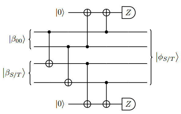
5.4.2 Logical Hadamard
Figure 5.14 gives the construction of our fault-tolerant logical Hadamard. The teleportation scheme requires the ancillary input of , as well as the use of the logical cphase gadget , whose fault-tolerant preparation was described in Sec. 5.3.2.

In Fig. 5.14, a logical cphase gadget is applied to the incoming logical (data) state and the ancillary input state . The data qubits are then measured in the basis, using our measurement gadget. Depending on the outcome of the measurement, the remaining four qubits (originally ancillas, but now the data qubits after the teleportation) end up in one of two states: or . In the latter case, we apply a corrective logical gadget to the outgoing state.
This logical Hadamard gate is fault-tolerant in the following sense: The gadget in Fig. 5.14 with at most single damping fault teleports an incoming state with no-error to an output with upto one single-qubit damping error. The teleportation gadget without any faults, teleports an input with upto one single-qubit damping error to an output with at most one single-qubit damping error. This holds simply due to the fact the Hadamard gadget is constructed from the fault-tolerant basic encoded gadgets described in Sec. 5.3, each tolerant to a single damping error.
5.4.3 Logical and gates
We provide the teleportation circuits for the logical and gadgets in Fig. 5.15 and Fig. 5.16 respectively. Like the logical , these circuits are composed of elementary encoded gadgets described in Sec. 5.3, which can be realized fault-tolerantly.


In both cases, the state denotes the state of the incoming logical (data) qubits. In both cases, this state is acted upon by the logical gadget, followed by a logical cphase gate applied to and the appropriate ancillary input state . In both cases, the data qubits are measured in the basis, which teleports the desired state to the ancilla block, upto a logical operation.
The final step involves a conditional logical operation on the remaining qubits. In the case of the gadget, this conditional operation is , whereas in the case of the gadget, the conditional logical operation to be implemented is . Once again, the fault tolerance of the logical and gadgets follows from the fact that they are composed of basic encoded gadgets which are all known to be tolerant to single damping errors.
5.5 Pseudothreshold calculation
The reliability of a fault tolerance scheme is quantified by its error threshold, which refers to that critical value of the error rate, , at which the fault-tolerant protocol fails to perform any better than its unencoded version. If refers to the unencoded error rate, and if the fault-tolerant procedure can correct upto errors, then the failure rate of a fault-tolerant circuit is given by , where refers to the number of ways in which a unit can have two faults and thus propagate an output which is not correctable.
The critical error threshold is then obtained as , for the that solves,
| (5.12) |
Since this value in Eq. 5.12 describes the reliability of the scheme at just one level of encoding, we may think of it as a pseudo-threshold. This is a key departure from the standard notion of a fault tolerance threshold which is defined for an entire class of codes, by concatenating a given code multiple times [aliferis].
5.5.1 Memory Pseudothreshold

We first calculate such a pseudothreshold for a memory unit comprising a pair of ec gadgets interlaced with identity gates or rests, as shown in the Fig. 5.17. By explicit enumeration of the pairs of faults, referred to as malignant pairs, that lead to errors of in the output state, we obtain,
| (5.13) |
We refer to Appendix for the details of the calculation.
5.5.2 Computational Pseudothreshold
In order to obtain a computational pseudothreshold, we go beyond our encoded gadgets to construct extended units, which take into account both incoming errors as well as all faults occurring within a given gadget. The extended unit with the maximum number of malignant pairs determines the computational pseudothreshold. In our case, we have determined by exhaustive check that an extended cphase unit, shown in Fig. 5.18, is the unit that determines the error threshold. The extended cphase unit comprises of the encoded cphasegadget in Fig. 5.10, and ec units appended before each block of the encoded gadget.

In order to compute the pseudothreshold of this extended unit, we first enumerate the number of malignant pairs of damping faults leading to an output that is not correctable in the extended cz unit, assuming that the incoming state has no errors. We first label the different blocks that constitute the extended unit, as follows.
- 1.
ec1 - leading ec in block 1
- 2.
ec2 - leading ec in block 2
- 3.
cz gadget
- 4.
eca +
- 5.
ecb +
We can then represent the number of malignant pairs via a matrix whose rows and columns correspond to each block in Fig. 5.18, with the entries of the matrix denoting the total malignant pair contributions from the respective blocks. We merely note the final numbers here and refer to Appendix for the detailed enumeration of malignant pairs for every pair of blocks.
The total number of malignant pairs of damping errors is simply the sum of the entries of the matrix. Apart from the pairs of damping errors, we also need to keep track of the phase errors, and we argue in Appendix that there are malignant fault locations for the phase errors.
The total number of malignant pairs due to damping errors and malignant fault locations due to errors is given by, , leading to a computational pseudothreshold of
5.6 Conclusion
We develop a fault-tolerant scheme specific to the amplitude-damping channel, using the -qubit code. We construct gadgets, namely, the error correction unit, a universal gate set, and a two-qubit gate which are tolerant against single-qubit damping errors. Our constructions show that achieving fault tolerance using channel-adapted codes for nontrivial, non-Pauli noise models like amplitude-damping channel poses interesting challenges, and often leads to counter-intuitive results when viewed from the standpoint of the well established principles of quantum fault tolerance. For instance, although the logical two-qubit cnot gadget is transversal, it is not tolerant to single damping errors, thus violating the wisdom gained from standard fault tolerance schemes for Pauli channels based on stabilizer codes.
The structure of the non-Pauli noise dictates our choice of fault-tolerant gate gadgets. Thus, the transversal two-qubit cphase gadget and three-qubit ccz gadget turn out to be a naturally favoured set since they can be made tolerant against single damping errors. When it comes to single-qubit damping errors, we do not obtain transversal constructions for the code; rather, we have to rely on a teleportation-based scheme to implement the Hadamard gadget, and gadgets that are fault-tolerant.
Finally, we obtain a rigorous estimate on the level- pseudo threshold for the memory unit as and cphase-exrec unit of , by explicitly enumerating the malignant pairs of faults. We present an updated, extensive fault-tolerant scheme in Ref. [ak_ft] which takes into account the back-action errors besides single-qubit damping errors. While our work presents a first step towards achieving fault tolerance against a specific non-Pauli noise model, the ultimate goal would be to obtain a true fault tolerance threshold via concatenation or using surface codes. Whether such a concatenated scheme can be developed entirely using channel-adapted codes such as the code, or whether this would require us to concatenate the code with a suitable general purpose code remains an interesting open question. Another immediate question is whether gadgets that are tolerant to amplitude-damping noise can be constructed using -d Bacon-shor code [renes]. Such a code might lead to a genuine fault tolerance threshold for amplitude-damping noise.
Chapter 6 Summary and Future Scope
Our thesis work entails a study of three interesting aspects centered around channel-adapted quantum codes, namely,
- (a)
Construction: we have proposed an efficient numerical way to search for channel-adapted codes and demonstrated its usefulness in the case of amplitude-damping noise [ak_cartan].
- (b)
Application: we have shown how channel-adapted codes may be used in the context of the quantum state transfer protocol to obtain better fidelities over longer spin chains [ak_statetransfer].
- (c)
Fault tolerance: we have developed a fault-tolerant scheme comprising a universal gate set and error-correction units, based on the -qubit code adapted to amplitude-damping noise [ak_ft].
The work presented in this thesis has several novel aspects and original results. For instance, the use of the Cartan form for finding good codespaces (Chapter 3) to protect quantum information is novel and leads to an efficient numerical procedure to search for quantum codes. Similarly, in Chapter 5, a new paradigm has been developed for quantum fault tolerance using channel-adapted quantum error correction, including several novel circuit constructions.
Our work opens up several directions of research. It would be interesting to study how the numerical procedure elaborated in Chapter 3 extends to the case of passive error suppression techniques such as decoherence-free subspaces (DFS) and noiseless subsystems(NS). Recently, [wang] proposed a numerical procedure to search for the existence of DFS/NS in noise models with and without perturbations. We note here that it is indeed straightforward to extend our search procedure to check for the existence of DFS for a given noise model. For example, motivated by existence of a DFS for correlated amplitude-damping noise [correlated_AD] on two qubits, we examined the case of the -qubit and -qubit correlated amplitude-damping noise channels. Preliminary results suggest that our unstructured search procedure, where we make use of a full, unstructured parameterization of the encoding unitary, may work well and can identify the subspaces corresponding to a DFS for both cases.
Channel-adapted codes are expected to have a wide variety of applications in different quantum information processing tasks. We have demonstrated one such application in the context of quantum state transfer over -d spin chains in Chapter 4. While our work has focussed on spin-preserving Hamiltonians, our protocol can still be extended to study more general Hamiltonians based on realistic implementations. For example, the Josephson junction arrays with a more general non-spin preserving Hamiltonian [lyakhov] gives rise to an arbitrary noise channel. In such a case our state transfer protocol with channel-adapted codes could be more useful over the perfect QEC protocols.
The important open problem of achieving fault tolerance using a channel-adapted code has been studied in Chapter 5. The problem of constructing fault-tolerant gadget set for a non-Pauli noise model is a counter-intuitive, challenging task, deviating from the standard fault-tolerant constructions that deal with Pauli errors and use perfect codes. While we study fault tolerance using a specific channel-adapted code, namely,the code [leung], it would be interesting to see if there are other codes tailormade to specific noise models which maybe used in this regard. For example, an immediate question is whether gadgets that are tolerant to amplitude-damping noise can be constructed using the -d Bacon-shor code [renes]. Such a code might allow us to build a universal fault-tolerant scheme, leading to a genuine fault tolerance threshold for amplitude-damping noise.
Appendix A Channel-adapted codes for the amplitude-damping channel
A.1 Nelder-Mead search algorithm
The Nelder-Mead algorithm [nelderpaper, NumericalRecipes] to search for optimal encoding proceeds through the following steps.
- 1.
We first create a -fold simplex for a parameter search space, with each of the vertex initialized to a unitary by sampling the parameters of the unitary from a uniform distribution over . We also pick an initial code space spanned by . At each vertex, we then obtain,
where span the code space at each vertex .
- 2.
Each iteration of the Nelder-mead algorithm proceeds via the following steps.
- (i)
Sort : Each vertex is given by a set of real parameters , describing the unitary according to the Cartan decomposition given in Sec. 3.3. The objective function, which is the fidelity-loss function given in Eq. 3.10 is then evaluated at each vertex for as , and then the set is sorted such that,
(A.1) where is the minimum value and is the maximum value of the fidelity-loss. The centroid corresponding to this set of vertices after sorting is obtained as given below,
(A.2) - (ii)
Reflect : We now obtain as follows,
(A.3) where the constant, . If , replace with .
- (iii)
Expand: If , then obtain,
(A.4) where the constant, . If , replace with , otherwise replace with .
- (iv)
Contract: If , then obtain,
(A.5) where the constant, . If , replace with , otherwise go to step (v).
- (v)
Shrink: for , replace
(A.6) where the constant, . We again go to step (i) .
- (i)
Thus the algorithm proceeds by generating newer simplices at every step and flows towards the optimum. Also, note that at each step a new is generated at vertex, giving a new code space spanned by
The search is terminated once the optimum is attained for the desired accuracy level.
A.2 Structured Codes and Encoding Circuits
Here, we describe simple circuits by means of which a structured encoding of the form given in Eq. (3.16) can be implemented. Recall that the Cartan decomposition for such a unitary is given by,
| (A.7) |
where the unitary operators are constructed from elements of an Abelian subgroup of the -fold Pauli group. For the case of , these operators are given by [see Eq. (3.14)],
| (A.8) | |||||
Following a simple prescription in [swaddle], we can construct quantum circuits to implement and by suitably combining the simple circuits given in Fig. . The full encoding unitary given in Eq. (A.7) is then composed from the circuits for , and as given in Fig. .
(a)