∎

Singular Value Perturbation and Deep Network Optimization

Rudolf H. Riedi Affiliation: Mathematics Department, HES-SO The University of Applied Sciences of Western Switzerland
Fribourg, Switzerland Randall Balestriero Affiliation: Meta AI, FAIR
NYC, USA Richard G. Baraniuk Affiliation: Department of Electrical and Computer Engineering
Rice University, Houston, TX, 77005 USA

Abstract

We develop new theoretical results on matrix perturbation to shed light on the impact of architecture on the performance of a deep network. In particular, we explain analytically what deep learning practitioners have long observed empirically: the parameters of some deep architectures (e.g., residual networks, ResNets, and Dense networks, DenseNets) are easier to optimize than others (e.g., convolutional networks, ConvNets). Building on our earlier work connecting deep networks with continuous piecewise-affine splines, we develop an exact local linear representation of a deep network layer for a family of modern deep networks that includes ConvNets at one end of a spectrum and ResNets, DenseNets, and other networks with skip connections at the other. For regression and classification tasks that optimize the squared-error loss, we show that the optimization loss surface of a modern deep network is piecewise quadratic in the parameters, with local shape governed by the singular values of a matrix that is a function of the local linear representation. We develop new perturbation results for how the singular values of matrices of this sort behave as we add a fraction of the identity and multiply by certain diagonal matrices. A direct application of our perturbation results explains analytically why a network with skip connections (such as a ResNet or DenseNet) is easier to optimize than a ConvNet: thanks to its more stable singular values and smaller condition number, the local loss surface of such a network is less erratic, less eccentric, and features local minima that are more accommodating to gradient-based optimization. Our results also shed new light on the impact of different nonlinear activation functions on a deep network’s singular values, regardless of its architecture.

Keywords:

Deep Learning, Optimization Landscape, Perturbation Theory, Singular Values
Dedication We dedicate this paper to Prof. Ron DeVore to celebrate his 80th birthday and his lifetime of achievements in approximation theory.

1 Introduction

Deep learning has significantly advanced our ability to address a wide range of difficult inference and approximation problems. Today’s machine learning landscape is dominated by deep (neural) networks (DNs) lecun2015deep, which are compositions of a large number of simple parameterized linear and nonlinear operators, known as layers. An all-too-familiar story of late is that of plugging a DN into an application as a black box, learning its parameter values using gradient descent optimization with copious training data, and then significantly improving performance over classical task-specific approaches.

Over the past decade, a menagerie of DN architectures has emerged, including Convolutional Neural Networks (ConvNets) that feature affine convolution operations lecun1995convolutional, Residual Networks (ResNets) that extend ConvNets with skip connections that jump over some layers he2016deep, Dense Networks (DenseNets) with several parallel skip connections huang2017densely, and beyond. A natural question for the practitioner is: Which architecture should be preferred for a given task? Approximation capability does not offer a point of differentiation, because, as their size (number of parameters) grows, these and most other DN models attain universal approximation capability daubechies2021neural.

Practitioners know that DNs with skip connections, such as ResNets and DenseNets, are much preferred over ConvNets, because empirically their gradient descent learning converges faster and more stably to a better solution. In other words, it is not what a DN can approximate that matters, but rather how it learns to approximate. Empirical studies li2018visualizing have indicated that this is because the so-called loss landscape of the objective function navigated by gradient descent as it optimizes the DN parameters is much smoother for ResNets and DenseNets as compared to ConvNets (see Figure 1). However, to date there has been no analytical work in this direction.

In this paper, we provide the first analytical characterization of the local properties of the DN loss landscape that enables us to quantitatively compare different DN architectures. The key is that, since the layers of all modern DNs (ConvNets, ResNets, and DenseNets included) are continuous piecewise-affine (CPA) spline mappings reportRB; balestriero2018spline, the loss landscape is a continuous piecewise function of the DN parameters. In particular, for regression and classification problems where the DN approximates a function by minimizing the $\ell_{2}$ -norm squared-error, we show that the loss landscape is a continuous piecewise quadratic function of the DN parameters. The local eccentricity of this landscape and width of each local minimum basin is governed by the singular values of a matrix that is a function of not only the DN parameters but also the DN architecture. This enables us to quantitatively compare different DN architectures in terms of their singular values.

Let us introduce some notation to elaborate on the above programme. We study state-of-the-art DNs whose layers $f_{k}$ comprise a nonlinear, continuous piecewise-linear activation function $\phi$ that is applied element-wise to the output of an affine transformation. We focus on the ubiquitous class of activations $\phi(t)=\max(\eta t,t)$ , which yields the so-called rectified linear unit (ReLU) for $\eta=0$ , leaky-ReLU for small $\eta\geq 0$ , and absolute value for $\eta=-1$ goodfellow2016deep. In an abuse of notation that is standard in the machine learning community, $\phi$ can also operate on vector inputs by applying the above activation function to each coordinate of the vector input separately. Focusing for this introduction on ConvNets and ResNets (we deal with DenseNets in Section 3), denote the input to layer $k$ by ${z}_{k}$ and the output by ${z}_{k+1}$ . Then we can write

{z}_{k+1}=f_{k}({z}_{k}):=\phi_{k}(W_{k}{z}_{k}+b_{k})+\rho{z}_{k},

(1)

where $W_{k}$ is an $n\times n$ weight matrix and $b_{k}$ is a vector of offsets.¹¹ 1 Without loss of generality, we assume that all $W_{k}$ are square. Rectangular $W_{k}$ are easily handled by extending with zeros. Typically $W_{k}$ is a (strided) convolution matrix. The choice $\rho=0$ corresponds to a ConvNet, while $\rho=1$ corresponds to a ResNet.

Refer to caption — Figure 1: Optimization loss landscape of two deep networks (DNs) along a 2D slice of their parameter space (from li2018visualizing). (left) Convolutional neural network (ConvNet) with no skip connections. (right) Residual network (ResNet) with skip connections. This paper develops new matrix perturbation theory tools to understand these landscapes and in particular explain why skip connections produce landscapes that are less erratic, less eccentric, and feature local minima that are more accommodating to gradient-based optimization. Used with permission.

Previous work balestriero2018spline; reportRB has demonstrated that the operator $f_{k}$ is a collection of continuous piecewise-affine (CPA) splines that partition the layer’s input space into polytopal regions and fit a different affine transformation on each region with the constraint that the overall mapping is continuous. This means that, locally around the input $z_{k}$ and the DN parameters $W_{k},b_{k}$ , (1) can be written as

{z}_{k+1}=D_{k}W_{k}{z}_{k}+D_{k}b_{k}+\rho{z}_{k},

(2)

where the diagonal matrix $D_{k}$ contains 1s at the positions where the corresponding entries of $W_{k}{z}_{k}+b_{k}$ are positive and $\eta$ where they are negative.

In supervised learning, we are given a set of $G$ labeled training data pairs $\{x^{(g)},y^{(g)}\}_{g=1}^{G}$ , and we tune the DN parameters $W_{k},b_{k}$ such that, when datum $x^{(g)}$ is input to the DN, the output $\widehat{y}^{(g)}$ is close to the true label $y^{(g)}$ as measured by some loss function $L$ . In this paper, we focus on the $\ell_{2}$ -norm squared-error loss averaged over a subset of the training data (called a mini-batch)

L:=\frac{1}{G}\sum_{g=1}^{G}\left\|y^{(g)}-\widehat{y}^{(g)}\right\|_{2}^{2}.

(3)

Standard practice is to use some flavor of gradient descent to iteratively reduce $L$ by differentiating with respect to $W_{k},b_{k}$ . For ease of exposition, we focus our analysis first on the case of fully stochastic gradient descent that involves only a single data point per gradient step (i.e., $G=1$ ), meaning that we iteratively minimize

L^{(g)}:=\left\|y^{(g)}-\widehat{y}^{(g)}\right\|_{2}^{2}

(4)

for different choices of $g$ . We then extend our theoretical results to arbitrary $G>1$ in Section 3.6. Let ${z}_{k}^{(g)}$ denote the input to the $k$ -th layer when the DN input is $x^{(g)}$ . Using the CPA spline formulation (2), it is easy to show (see (46)) that, for fixed $y^{(g)}$ , the loss function $L^{(g)}$ is continuous and piecewise-quadratic in $W_{k},b_{k}$ .

The squared-error loss $L^{(g)}$ is ubiquitous in regression tasks, where $y^{(g)}$ is real-valued, but also relevant for classification tasks, where $y^{(g)}$ is discrete-valued. Indeed, recent empirical work hui21 has demonstrated that state-of-the-art DNs trained for classification tasks using the squared-error loss perform as well or better than the same networks trained using the more popular cross-entropy loss.²² 2 We note in passing that one can use the techniques developed in this paper to show that the cross-entropy loss is continuous and piecewise-cross-entropic in $W_{k},b_{k}$ . Analysis of the local Hessian of this piecewise loss would lead to the same conclusion as with the squared-error loss, namely that the loss landscapes of ResNets/DenseNets are strictly better behaved than those of ConvNets. We leave the details of this analysis for future work.

We can characterize the local geometric properties of this piecewise-quadratic loss surface as follows. First, without loss of generality, we simplify our notation. For the rest of the paper, we label the layer of interest by $k=0$ and suppress the subscript $0$ (i.e., $W_{0}\rightarrow W$ ); we assume that there are $p$ subsequent layers ( $f_{1},\dots,f_{p}$ ) between layer 0 and the output $\widehat{y}$ . Optimizing the weights $W$ of layer $f$ with training datum $x^{(g)}$ that produces layer input $z^{(g)}$ requires the analysis of the DN output $\widehat{y}$ , due to the chain rule calculation of the gradient of $L$ with respect to $W$ . (As we discuss below, there is no need to analyze the optimization of $b$ .) For further simplicity, we suppress the superscript ${(g)}$ that enumerates the training data whenever possible. We thus write the DN output as

\widehat{y}=M(\rho)DW{z}+B

(5)

where

M(\rho)=D_{p}W_{p}\cdots D_{1}W_{1}+\rho\,{\rm Id}

(6)

collects the combined effect of applying $W_{k}$ in subsequent layers $f_{k}$ , $k=1,\dots,p$ , and $B$ collects the combined offsets. Note that $z$ reflects the influence of the training datum combined with the action of the layers preceding $f$ and can be interpreted as the input to the shallower network consisting of layers $f,f_{1},\dots,f_{p}$ . This justifies using the index $0$ for the layer under consideration.

Using this notation and fixing $b$ as well as the input ${z}$ , the piecewise-quadratic loss function $L$ can be written locally as a linear term in $W$ plus a quadratic term in $W$ , which can be written as a quadratic form featuring matrix $Q$ (see Lemma 8)

{z}^{T}W^{T}D^{T}M(\rho)^{T}M(\rho)DW{z}=w^{T}Q^{T}Qw.

(7)

Here, $w$ denotes the columnized vector version of the matrix $W$ .

The semi-axes of the ellipsoidal level sets of the local quadratic loss (7) are determined by the singular values of the matrix $Q$ , which we can write as $s_{i}\cdot|{z}[j]|$ according to Corollary 9, with $s_{i}=s_{i}(MD)$ the $i$ -th singular value of the linear mapping $MD$ and ${z}[j]$ the $j$ -th entry in the vector ${z}$ . The eccentricity of the ellipsoidal level sets is governed by the condition number of $Q$ which, therefore, factors as

\kappa(Q)=\frac{\max_{i}s_{i}(MD)}{\min_{i}^{*}s_{i}(MD)}\,\cdot\,\frac{\max_{j}{|z}[j]|}{\min_{j}^{*}|{z}[j]|}=\kappa(MD)\cdot\kappa(\mbox{\rm diag}({z})).

(8)

Here, $\min^{*}$ denotes the minimum after discarding all vanishing elements (cf. (53)). In this paper we focus on the effect of the DN architecture on the condition number of the matrix $MD$ representing the action of the subsequent layers, which is

\kappa(MD)=\frac{\max_{i}s_{i}(MD)}{\min_{i}^{*}s_{i}(MD)}.

(9)

However, the factorization in (8) provides insights into the role played by the training datum ${z}$ (see Corollary 9). Extensions of these results to batches $(G>1)$ are found in Section 3.6. (We note at this point that the optimization of the offset vector $b$ has no effect on the shape of the loss function.)

For a fixed set of training data (i.e., fixed ${x}$ ), the difference between the loss landscapes of a ConvNet and a ResNet is determined soley by $\rho$ in (6). Therefore, we can make a fair, quantitative comparison between the loss landscapes of the ConvNet and ResNet architectures by studying how the singular values of the linear mapping $M(\rho)D$ evolve as we move infinitesimally from a ConvNet ( $\rho=0$ ) towards a ResNet ( $\rho=1$ ).

Addressing how the singular values and condition number of the linear mapping $M(\rho)D$ (and hence the DN optimization landscape) change when passing from $\rho=0$ towards $\rho=1$ requires a nontrivial extension of matrix perturbation theory. Our focus and main contributions in this paper lie in exploring this under-explored territory.³³ 3 A closely related situation occurs in Tikhonov regularization, where Id is added to $M^{T}M$ in order to regularize the ill-posed problem $Mx=b$ . Our analysis technique is new, and so we dedicate most of the paper to its development, which is potentially of independent interest.

We briefly summarize our key theoretical findings from Sections 2–6 and our penultimate result in Theorem 22. We provide concrete bounds on the growth or decay of the singular values of any square matrix $M_{o}=M(0)$ when it is perturbed to $M(\rho)=M_{o}+\rho\,{\rm Id}$ by adding a multiple of the identity $\rho\,{\rm Id}$ for $0\leq\rho\leq 1$ . The bounds are in terms of the largest and smallest eigenvalues of the symmetrized matrix $M_{o}^{T}+M_{o}$ . The behavior of the largest singular value under this perturbation can be controlled quite accurately in the sense that random matrices tend to follow the upper bound we provide quite closely with high probability. For all other singular values, we require that they be non-degenerate, meaning that they have multiplicity $1$ for all but finitely many $\rho$ , a property that holds for most matrices in a generic sense (see Lemma 12). Further, we establish bounds for arbitrary singular values that do not hinge on the assumption of multiplicity $1$ but that are somewhat less tight.

Our new perturbation results enable us to draw three rigorous conclusions regarding the optimization landscape of a DN. First, with regards to network architecture, we establish that the addition of skip connections improves the condition number of a DN’s optimization landscape. To this end, we point out that no guarantees on the piecewise-quadratic optimization landscape’s condition number are available for ConvNets; in particular, $\kappa(M(0))$ can take any value, even if the entries of $M(0)$ are bounded. However, as we move from ConvNets ( $\rho=0$ ) towards networks with skip connections such as ResNets and DenseNets ( $\rho>0$ ), bounds on $\kappa(M(\rho))$ become available. For an appropriate random initialization of the weights and a wide network architecture (large $n$ ), we show that the condition number of a ResNet ( $\rho=1$ ) is bounded above asymptotically by just $3$ (see (121), (122), and (128)). Second, for the particular case of DNs employing absolute value activation functions, we show that the relevant condition number is easier to control than for ReLU activations, that is, absolute value requires less restrictive assumptions on the entries of $M$ in order to bound the condition number. For absolute value, we also prove that the condition number of $M(1)$ (ResNet) is smaller than that of $M(0)$ (ConvNet) with probability asymptotically equal to $1$ . Third, with regards to the influence of the training data, we prove that extreme values of the data negatively affect the performance of linear least squares and that this impact is tempered when applying mini-batch learning due to its inherent averaging.

In the context of DN optimization, these results demonstrate that the local loss landscape of a DN with skip connections (e.g., ResNet, DenseNet) is better conditioned than that of a ConvNet and thus less erratic, less eccentric, and with local minima that are more accommodating to gradient-based optimization, particularly when the weights in $W$ are small. This is typically the case at the initialization of the optimization glorot2011deep and often remains true throughout training gal2016dropout. In particular, our results also provide new insights into the best magnitude to randomly initialize the weights at the beginning of learning in order to reap the maximum benefit from a skip connection architecture.

This paper is organized as follows. Section 2 introduces our notation and provides a review of existing useful results on the perturbation of singular values. Section 3 overviews our prior work establishing that CPA DNs can be viewed as locally linear and leverages this essential property to identify the singular values relevant for understanding the shape of the quadratic loss surface used in gradient-based optimization. Section 4 develops the perturbation results needed to capture the influence on the singular values when adding a skip connection, i.e., when passing from $M_{o}$ to $M_{o}+{\rm Id}$ . In particular, we provide bounds on the condition number of $M_{o}+\rho{\rm Id}$ in terms of the largest singular value of $M_{o}$ and the largest and the smallest eigenvalue of $M_{o}^{T}+M_{o}$ . Section 5 combines the findings of Sections 3 and 4 to show that a layer with a skip connection and weights bounded by an appropriate constant will have a bounded condition number. Clearly, this applies to weights drawn from a uniform distribution. Section 6 is dedicated to a ResNet layer with random weights of bounded standard deviation. Here, we establish bounds on the condition number of the corresponding ResNet and on the probability with which they hold, explicitly in terms of the width $n$ of the network. Further, we provide convincing numerical evidence that the asymptotic bounds apply in practice for widths as modest as $n\geq 5$ . We conclude in Section 7 with a synthesis of our results and perspectives on future research directions. All proofs are provided within the main paper. Various empirical experiments sprinkled throughout the paper support our theoretical results.

2 Background

2.1 Notation

Singular values. Let $A$ be a $n\times n$ -matrix, and let $\|u\|$ denote the $\ell_{2}$ -norm of the vector $u$ . All products are to be understood as matrix multiplications, even if the factors are vectors. Vectors are always column vectors.

Let $u_{i}$ denote a unit-eigenvector of $A^{T}A$ to its eigenvalue $\lambda_{i}=\lambda_{i}(A^{T}A)$ such that the vectors $u_{i}$ ( $i=1\ldots n$ ) form an orthonormal basis.

The singular values of $A$ are defined as the square roots of the eigenvalues of ${A}^{T}{A}$

s_{i}=s_{i}(A)=\sqrt{\lambda_{i}({A}^{T}{A})}=\|{A}u_{i}\|.

(10)

Note that the singular values are always real and non-negative valued, since

0\leq\|{A}u_{i}\|^{2}=u_{i}^{T}{A}^{T}{A}u_{i}=\lambda_{i}u_{i}^{T}u_{i}=\lambda_{i}.

(11)

For reasons of definiteness, we take the eigenvalues of ${A}^{T}{A}$ , and thus the singular values of ${A}$ to be ordered by size: $s_{1}\geq\ldots\geq s_{n}$ .

Singular vectors. The vectors $u_{i}$ are called right singular vectors of ${A}$ . The left singular vectors of ${A}$ are denoted $v_{i}$ and are defined as an orthonormal basis with the property that

{A}u_{i}=s_{i}v_{i}\qquad\mbox{and}\qquad{A}^{T}v_{i}=s_{i}u_{i}.

(12)

Such a basis of left-singular vectors always exists.

SVD. Collecting the right singular vectors $u_{i}$ as columns into an orthogonal matrix $U$ , the left singular vectors $v_{i}$ into an orthogonal matrix $V$ , and the singular values $s_{i}$ into a diagonal matrix $\Sigma$ in corresponding order, we obtain the Singular Value Decomposition (SVD) of ${A}=V\Sigma U^{T}$ .

Eigenvectors. Note that ${A}$ may have eigenvectors that differ from the singular vectors. In particular, eigenvectors are not always orthogonal onto each other. Clearly, if ${A}$ is symmetric then the eigenvectors and right-singular vectors coincide and every eigenvalue $r_{i}$ of ${A}$ corresponds to a singular value $s_{i}=|r_{i}|$ . However, to avoid confusion, we will refrain from referring to the eigenvalues and the singular values of the same matrix whenever possible.

Smooth matrix deformations. Consider a family of $n\times n$ matrices ${A}(\rho)$ , where the variable $\rho$ in assumed to lie in some interval $I$ . We say that the family ${A}(\rho)$ is $\mathcal{C}^{m}(I)$ if all its entries are $\mathcal{C}^{m}(I)$ , with $m=0$ corresponding to being continuous and $m=1$ to continuously differentiable. If ${A}$ is $\mathcal{C}^{m}(I)$ , then so is ${A}^{T}{A}$ .

We denote the matrix of derivatives of the entries of ${A}$ by ${A}^{\prime}(\rho)=\frac{d}{d\rho}{A}(\rho)$ .

Multiplicity of singular values Denote by $S_{i}\subset I$ the set of $\rho$ values for which $s_{i}$ is a simple singular value:

S_{i}=\{\rho\in I\,:\,s_{i}(\rho)\neq s_{j}(\rho)\mbox{ for all $j\neq i$}\}.

(13)

For later use, let

S_{i}^{*}=\{\rho\in S_{i}\,:\,s_{i}(\rho)\neq 0\}.

(14)

For completeness, we mention an obvious fact that follows from the SVD:

s_{i}({A})=s_{i}\!\left({A}^{T}\right).

(15)

2.2 Singular values under additive perturbation

A classical result that will prove to be key in our study is due to Wielandt and Hoffman Wielandt_Hoffman. It uses the notion of the Frobenius norm $\|{A}\|_{F}$ of the $n\times n$ -matrix ${A}$ . Denoting the entries of ${A}$ by ${A}[i,j]$ and its singular values by $s_{i}({A})$ , it is well known that

\|{A}\|_{F}^{2}=\sum_{i,j=1}^{n}|{A}[i,j]|^{2}=\mbox{\rm trace}({A}^{T}{A})=\sum_{i=1}^{n}s_{i}^{2}({A}).

(16)

Proposition 1 (Wielandt and Hoffman)

Let ${A}$ and ${{\tilde{A}}}$ be symmetric $n\times n$ -matrices with eigenvalues ordered by size. Then

\sum_{i=1}^{n}\Big|\lambda_{i}({A})-\lambda_{i}({{\tilde{A}}})\Big|^{2}\leq\|{A}-{{\tilde{A}}}\|_{F}^{2}.

(17)

This result can easily be strengthened to read as follows.

Corollary 2 (Wielandt and Hoffman)

Let ${A}$ and ${{\tilde{A}}}$ be any $n\times n$ -matrices with singular values ordered by size. Then

\sum_{i=1}^{n}\Big|s_{i}({A})-s_{i}({{\tilde{A}}})\Big|^{2}\leq\|{A}-{{\tilde{A}}}\|_{F}^{2}.

(18)

Note that this result, as most others, holds actually also for rectangular matrices with the usual adjustments.

Proof

We establish Corollary 2. The $2n$ eigenvalues of the symmetric matrix

H_{A}=\left(\begin{array}[]{cc}0&{A}\\ {A}^{T}&0\end{array}\right)

(19)

are $s_{i}({A})$ with eigenvector $\frac{1}{\sqrt{2}}{v_{i}\choose u_{i}}$ and $-s_{i}({A})$ with eigenvector $\frac{1}{\sqrt{2}}{-v_{i}\choose u_{i}}$ . Also, $\|H_{A}\|_{F}^{2}=2\|{A}\|_{F}^{2}$ . Therefore, when applying Proposition 1 with $A$ replaced by $H_{A}$ and ${\tilde{A}}$ replaced by $H_{\tilde{A}}$ , we run through the left-hand side of (18) twice and in turn obtain twice the right-hand side.

Corollary 2. immediately implies a well-known result that will be key: the singular values of a matrix depend continuously on its entries, as we state next.

Lemma 3

If ${A}(\rho)$ is $\mathcal{C}^{0}(I)$ , then all its singular values $s_{i}(\rho)$ depend continuously on $\rho$ . Consequently, all $S_{i}$ in (13) and $S_{i}^{*}$ in (14) are then open.

Proof

To establish continuity, choose $\rho_{1}$ and $\rho_{2}$ arbitrary and apply Corollary 2 (in slight abuse of notation) with ${A}={A}(\rho_{1})$ and ${{\tilde{A}}}={A}(\rho_{2})$ .

As will become clear in the sequel, the main difficulty in establishing further results on the regularities of the singular values with elementary arguments and estimates lies in dealing with multiple zeros, i.e., with multiple singular values.

Also useful are some facts about the special role of the largest singular value.

Proposition 4 (Operator norm)

Let ${A}$ be a $n\times n$ -matrix. Then, its largest singular value is equal to its operator norm, and we have the following inequalities:

s_{1}({A})=\|{A}\|_{\rm Op}:=\max_{|x|=1}|Ax|\leq\|{A}\|_{F}\leq\sqrt{{\rm rank}({A})}\cdot\|{A}\|_{\rm Op}.

(20)

In particular, if ${A}$ is rank 1, then both norms coincide. Also, being a norm, the largest singular value satisfies

s_{1}({A}+{{\tilde{A}}})\leq s_{1}({A})+s_{1}({{\tilde{A}}})

(21)

for any matrices ${A}$ and ${{\tilde{A}}}$ .

Proof

The first equality follows from the fact that $s_{1}$ is the largest semi-axis of the ellipsoid that is the image of the unit-sphere. The first inequality follows from (16). The last inequality follows again from considering the aforementioned ellipsoid.

Another proof of the continuity of singular values is found in the well-known interlacing properties of singular values, which we adapt to our notation and summarize for the convenience of the reader (see, e.g. (Chafai, Theorem 6.1.3-5.)).

Proposition 5 (Interlacing)

Let ${A}$ and ${{\tilde{A}}}$ be $n\times n$ -matrices with singular values ordered by size.

•

(Weyl additive perturbation) We have:

$s_{i+j-1}({A})\leq s_{i}({{\tilde{A}}})+s_{j}({A}-{{\tilde{A}}}).$ (22)
•

(Cauchy interlacing by deletion) Let ${{\tilde{A}}}$ be obtained from ${A}$ by deleting $m$ rows or $m$ columns. Then

$s_{i}({A})\geq s_{i}({{\tilde{A}}})\geq s_{i+m}({A}).$ (23)

From (22) applied with $j=1$ , we note that the singular values are in fact uniformly continuous. Indeed, we have for any $i$ that

|s_{i}({A})-s_{i}({{\tilde{A}}})|\leq s_{1}({A}-{{\tilde{A}}})\leq\|{A}-{{\tilde{A}}}\|_{F}.

(24)

2.3 Singular values under smooth perturbation

We now turn to the study of how singular values of ${A}(\rho)$ change as a function of $\rho$ , thereby leveraging the concept of differentiability.

This can be done in several ways; the following computation is particularly simple and well known. Let $N(\rho)$ denote a family of symmetric $\mathcal{C}^{1}(I)$ matrices. Dropping all indices and variables $\rho$ for ease of reading, the eigenvalues and eigenvectors satisfy

\displaystyle Nu=\lambda u,\qquad u^{T}u=1.

(25)

Denoting the derivatives with respect to $\rho$ by $N^{\prime}$ , $\lambda^{\prime}$ and $u^{\prime}$ and assuming they exist, we obtain

\displaystyle N^{\prime}u+Nu^{\prime}=\lambda^{\prime}u+\lambda u^{\prime},\qquad u^{\prime T}u=u^{T}u^{\prime}=0.

(26)

We then left-multiply the first equality by $u^{T}$ and use the second equality to find

\displaystyle u^{T}N^{\prime}u+u^{T}Nu^{\prime}=\lambda^{\prime}u^{T}u+\lambda u^{T}u^{\prime}=\lambda^{\prime}.

(27)

Finally, as $N$ is symmetric we see that $u^{T}Nu^{\prime}=(Nu)^{T}u^{\prime}=\lambda u^{T}u^{\prime}=0$ , leading to

\lambda^{\prime}=u^{T}N^{\prime}u.

(28)

In quantum mechanics, the last equation is known as the Hellmann-Feynman Theorem and was discovered independently by several authors in the 1930s. It is known, though seldom mentioned, that the formula may fail when eigenvalues coincide. For further studies in this direction, we refer the interested reader to works in the field of degenerate perturbation theory.

For a proof of the Hellmann-Feynman Theorem, it is natural to consider the function $\Psi:{\rm I\mkern-2.5mu\nonscript\mkern-0.5muR}^{n+2}\to{\rm I\mkern-2.5mu\nonscript\mkern-0.5muR}^{n+1}$

\Psi(\rho,u,\lambda)=\left(\begin{array}[]{c}Nu-\lambda u\\ u^{T}u-1\end{array}\right),

(29)

where $u$ is an $n$ -dimensional column vector. The Implicit Function Theorem applied to $\Psi$ then yields the following result.

Theorem 6 (Hellmann-Feynman)

Assume $N(\rho)$ forms a family of symmetric $\mathcal{C}^{1}(I)$ matrices. Then, as a function of $\rho$ , each of its eigenvalues $\lambda_{i}=\lambda_{i}(\rho)$ is continuously differentiable where it is simple. Its derivative reads as

\lambda_{i}^{\prime}(\rho)=u_{i}^{T}N^{\prime}u_{i}.

(30)

Its corresponding right singular vector $u_{i}(\rho)$ can be chosen such that it becomes $\mathcal{C}^{1}(S_{i})$ as well.

If in addition to the assumptions of Theorem 6 the family $N$ is actually $\mathcal{C}^{m}(I)$ , then $\lambda_{i}(\rho)$ and $u_{i}(\rho)$ are $\mathcal{C}^{m}(S_{i})$ . From Hellmann-Feynmann we may conclude the following.

Corollary 7

Let ${A}(\rho)$ be $\mathcal{C}^{1}(I)$ . Assume that $S_{i}^{*}$ consists of isolated points only. Then, $s_{i}(A)$ and its left singular vector $v_{i}$ are $\mathcal{C}^{1}(S_{i}^{*})$ with

s^{\prime}_{i}(\rho)=u_{i}(\rho)^{T}{{A}^{\prime}(\rho)}^{T}v_{i}(\rho).

(31)

Simple examples show that the above results cannot be improved without stronger assumptions (see Example 1 below and Figure 2).

Proof

Apply Theorem 6 to the family $N={A}^{T}{A}$ . Note that $N^{\prime}={A}^{\prime T}{A}+{A}^{T}{A}^{\prime}$ and apply the chain rule to $\lambda_{i}=(s_{i}(\rho))^{2}$ to find the first equality of the following formula:

s^{\prime}_{i}=\frac{1}{2s_{i}}u_{i}^{T}({A}^{\prime T}{A}+{A}^{T}{A}^{\prime})u_{i}=\frac{1}{2s_{i}}2u_{i}^{T}{{A}^{\prime}}^{T}{A}u_{i}=u_{i}^{T}{{A}^{\prime}}^{T}v_{i}.

(32)

Also, we have $u_{i}^{T}{A}^{\prime T}{A}u_{i}=(u_{i}^{T}{A}^{\prime T}{A}u_{i})^{T}=u_{i}^{T}{A}^{T}{A}^{\prime}u_{i}$ , since this is a real-valued number. This implies the second equality in the formula above. Finally note that ${A}u_{i}=s_{i}v_{i}$ to complete the proof.

Example 1: The diagonal family $M=$ diag $(-4~~-2)+\rho$ Id is $\mathcal{C}^{\infty}({\rm I\mkern-2.5mu\nonscript\mkern-0.5muR})$ . When ordered by size, the eigenvalues of $N=M^{T}M$ are $\max((\rho-4)^{2},(\rho-2)^{2})$ and $\min((\rho-4)^{2},(\rho-2)^{2})$ . They are not differentiable where they coincide. In particular, the matrix norm of $N$ is not differentiable at $\rho=3$ . The singular values of $M$ are $s_{1}=\max(|\rho-4|,|\rho-2|)$ and $s_{2}=\min(|\rho-4|,|\rho-2|)$ ; they are not differentiable at their respective zeros. Also, the left singular vectors $v_{i}$ change sign at the zero of $s_{i}$ and so are not even continuous there (see Figure 2 for a similar example).

3 Singular Values in Deep Learning

In this section, we establish that the squared-error loss landscape of a deep network (DN) is governed locally by the singular values of the matrix of weights of a layer and that the difference between certain network architectures can be interpreted as a perturbation of this matrix. Combining this key insight with the perturbation theory of singular values for DNs, which will be developed in the sections to follow, will enable us to characterize the dependence of the loss landscape on the underlying architecture. Doing so, we will ultimately provide analytical insight into numerous phenomena that have been observed only empirically so far, such as the fact that so called ResNets he2016identity are easier to optimize than ConvNets lecun1995convolutional.

3.1 The continuous piecewise-affine structure of deep networks

The most popular DNs contain activation nonlinearities that are continuous piecewise-affine (CPA), such as the ReLU, leaky-ReLU, absolute value, and max-pooling nonlinearities goodfellow2016deep. To be more precise, let $f_{k}$ denote a layer of a DN. We will assume that it can be written as an affine map $W_{k}{z_{k}}+b_{k}$ followed by the activation $\phi_{k}$

{z_{k+1}}=f_{k}({z_{k}})=\phi_{k}(W_{k}{z_{k}}+b_{k}).

(33)

The entries of the matrix $W_{k}$ are called weights; the constant additive term $b_{k}$ is called the bias. More general settings can easily be employed; however, the above will be sufficient for our purpose. The above-mentioned, commonly used nonlinearities can be written in this form using

\phi_{k}(t)=\max(t,\eta t),

(34)

where the max is taken coordinate by coordinate. Clearly, any activation of the form (34) is continuous and piecewise linear, rendering the corresponding layer CPA (Fig. 3). The following choices for $\eta$ correspond to ReLU ( $\eta=0$ ) glorot2011deep, leaky-ReLU ( $0<\eta<1$ ) DBLP:journals/corr/XuWCL15 and absolute value bruna2013invariant ( $\eta=-1$ ) (see also reportRB; balestriero2018spline). In summary:

\left\{\begin{array}[]{ll}\eta>0&\mbox{leaky-ReLU}\\ \eta=0&\mbox{ReLU}\\ \eta=-1&\mbox{absolute value}\\ \end{array}\right.

(35)

For example, in two dimensions we obtain $\phi_{k}^{\rm(Abs)}(t_{1},t_{2})=(|t_{1}|,|t_{2}|)$ . We will consider only nonlinearities that can be written in the form (34). Such nonlinearities are in fact linear in each hyper-octant of space, and can be written as

\phi_{k}(t)=D_{k}t,

where $D_{k}$ is a diagonal matrix with entries that depend on the signs of the coordinates of the input $t=W_{k}{z_{k}}+b_{k}$ . The diagonal entries of $D_{k}$ equal either $1$ or $\eta$ depending on the hyper-octant.

Consequently, the input space of the layer $f_{k}$ is divided into regions that depend on $W_{k}$ and $b_{k}$ in which $f_{k}$ is affine and can be rewritten as

{z_{k+1}}=f_{k}({z_{k}})=\phi_{k}(W_{k}{z_{k}}+b_{k})=(D_{k}W_{k}){z_{k}}+D_{k}b_{k}.

(36)

By the linear nature of ${z_{k}}\mapsto W_{k}{z_{k}}$ , these regions of the input space ( ${z_{k}}$ -space) are piecewise linear. Concatenating several layers into a multi-layer $F({z_{1}})=f_{p}\circ\ldots\circ f_{1}({z_{1}})$ then leads to a subdivision of its input space into piecewise-linear regions (see Figure 3) in which $F$ is affine, a result due to balestriero2018spline; reportRB. In each linear region, this multi-layer can be written as

{z_{p+1}}=D_{p}W_{p}\ldots D_{1}W_{1}{z_{1}}+B_{p},

(37)

where all constant terms are collected in

B_{p}=D_{p}W_{p}\ldots D_{2}W_{2}b_{1}+D_{p}W_{p}\ldots D_{3}W_{3}b_{2}+\ldots+b_{p}.

(38)

A multi-layer can be considered to be an entire DN or a part of one.

Figure 3: Iterative partitioning of input space by three consecutive layers of a toy deep network (DN). The first layer maps

{\rm I\mkern-2.5mu\nonscript\mkern-0.5muR}^{2}

{\rm I\mkern-2.5mu\nonscript\mkern-0.5muR}^{3}

, producing three cuts and seven regions, with one lying outside the visualized region.

3.2 From ConvNets to ResNets and DenseNets, and learning

A DN with an architecture $F({z_{1}})=f_{p}\circ\ldots\circ f_{1}({z_{1}})$ as described above is called a Convolutional Network (ConvNet) lecun1995convolutional whenever the $W_{k}$ are circulant-block-circulant; otherwise it is called a multi-layer-perceptron. Without loss of generality, we will focus on ConvNets and their extensions, particularly ResNets and DenseNets, in this paper. While such architectures are responsible for the recent cresting wave of deep learning successes, they are known to be intricate to effectively employ when the number of layers $p$ large. This motivated research on alternative architectures.

When adding the input ${z_{k}}$ to the output $\phi_{k}(W_{k}{z_{k}}+b_{k})$ of a convolutional layer (a skip connection), one obtains a residual layer which can be written in each region of linearity as

{z_{k+1}}=f_{k}({z_{k}})=\phi_{k}(W_{k}{z_{k}}+b_{k})+{z_{k}}=(D_{k}W_{k}+{\rm Id}){z_{k}}+D_{k}b_{k}.

(39)

A DN in which all (or most) layers are residual is called a Residual Network (ResNet) he2016identity. Densely Connected Networks (DenseNets) huang2017densely allow the residual connection to bypass not just a single but multiple layers

{z_{p+1}}=(D_{p}W_{p}\ldots D_{1}W_{1}+{\rm Id}){z_{1}}+B_{p}.

(40)

All of the above DN architectures are universal approximators. Learning the per-layer weights of any DN architecture is performed by solving an optimization problem that involves a training data set, a differentiable loss function such as the squared-error or cross-entropy, and a weight update policy such as gradient descent. Hence, the key benefit of one architecture over another only emerges when considering the learning problem, and in particular gradient-based optimization.

3.3 Learning

We now consider the learning process for one particular layer of a DN. As we make clear below, for the comparison of different network architectures, it is sufficient to study each layer independently of the others. For ease of exposition, our analysis in Sections 3.3–3.5 also focuses on a single training data point, which corresponds to learning via fully stochastic gradient descent ( $G=1$ in the Introduction). We extend our analysis to the general case of mini-batch gradient descent ( $G>1$ ) in Section 3.6.

The layer being learned is $f_{0}$ ; however, for clarity we drop the index $0$ and use the notation

{{z_{1}}}=f(z)=\phi(Wz+b)=DWz+b.\qquad\qquad\qquad\qquad\,\mbox{(trained layer)}

(41)

The layers following $f$ are the only ones relevant in the study of learning layer $f$ . In fact, the previous layers transform the DN input into a feature map that, for the layer in question, can be seen as a fixed input. This part of the network will be denoted by $F=f_{p}\circ\ldots\circ f_{1}$ . In each partition region, it takes the form

\displaystyle{\widehat{y}}=MDWz+B.\qquad\qquad\qquad\,\mbox{(trained plus subsequent layers)}

(42)

Here, $B$ collects all of the constants, $D$ represents the nonlinearity of the trained layer in the current region, and $M$ collect the action of the subsequent layers $F$ . We use the parameter $\rho$ to distinguish between ConvNets and ResNets, with $\rho=0$ corresponding to convolution layers and $\rho=1$ to residual ones. The matrix $M=M(\rho)$ representing the subsequent layers $F$ becomes

	$\displaystyle M=M(\rho)$	$\displaystyle=$	$\displaystyle D_{1}W_{1}+\rho{\rm Id}~\qquad\qquad\qquad\qquad\,\mbox{(one layer)}$		(43)
	$\displaystyle M=M(\rho)$	$\displaystyle=$	$\displaystyle D_{p}W_{p}\cdots D_{1}W_{1}+\rho{\rm Id}.\qquad\qquad\mbox{(multi-layer)}$		(44)

As a shorthand, we will often write $M(\rho)=M_{o}+\rho{\rm Id}$ , where

M_{o}=M(0)=D_{p}W_{p}\cdots D_{1}W_{1}.

(45)

When saying “let $M_{o}$ be arbitrary” we mean that no restrictions on the factors in (45) are imposed except for the $D_{i}$ to be diagonal and the $W_{i}$ to be square. When choosing $D_{p}=\cdots=D_{1}=W_{p}=\cdots=W_{2}={\rm Id}$ and $W_{1}$ arbitrary, we have $M_{o}=W_{1}$ arbitrary. So, there is no ambiguity in our usage of the term “arbitrary”.

3.4 Quadratic loss

We wish to quantify the advantage in training of a ResNet architecture over a ConvNet one. We consider a quadratic loss function such as the squared-error as mentioned in the Introduction (cf. (4); we drop the superscript ${(g)}$ ):

L^{(g)}:=\left\|y-\widehat{y}\right\|_{2}^{2}=(y-\widehat{y})^{T}(y-\widehat{y})=\left\|y\right\|_{2}^{2}-2y^{T}\widehat{y}+\left\|\widehat{y}\right\|_{2}^{2}.

(46)

In the above, we used that $y^{T}\widehat{y}=\left(y^{T}\widehat{y}\right)^{T}=\widehat{y}^{T}y$ , since this is a real number.

Recalling that the DN is a continuous piecewise-affine operator and fixing all parameters except for $W$ , we can locally write $\widehat{y}=MDW{z}+B$ for all $W$ in some region $\mathcal{R}$ of $F$ (cf. (4); $z$ is the input to $f$ produced by the datum $x^{(g)}$ ). Writing $\left\|\widehat{y}\right\|_{2}^{2}=\widehat{y}^{T}\widehat{y}$ , we find that the loss can be viewed as an affine term $P(W)$ with $P$ a polynomial of degree $1$ plus a quadratic term $\|MDW{z}\|_{2}^{2}$

\displaystyle L^{(g)}=P(W)+\|MDW{z}\|_{2}^{2}\qquad(W\in\mathcal{R}).

(47)

We stress once more that all parameters are fixed except for $W$ . Denote by $W_{o}=W_{o}(\rho,\mathcal{R})$ the minimum of the function $h(W)=P(W)+\|MDW{z}\|_{2}^{2}$ ( $W$ arbitrary), which may very well lie outside $\mathcal{R}$ . Writing $\Delta W=W-W_{o}$ and developing $h$ into its Taylor series at $W_{o}$ , we find $h(W)=h(W_{o})+\|MD\Delta W{z}\|_{2}^{2}$ , since all first order derivatives of $h$ vanish at $W_{o}$ .

It is worthwhile noting that the region $\mathcal{R}$ does not change when changing the value of $\rho$ in $M=M(\rho)$ , since $D\Delta W{z}$ does not depend on $\rho$ . From this, writing $c=h(W_{o})$ for short, we obtain for any $\rho$

\displaystyle L^{(g)}=c+\|M(\rho)D\Delta W{z}\|_{2}^{2}\qquad(W\in\mathcal{R}).

(48)

This means that the loss surface is in each region $\mathcal{R}$ of $F$ is a part of an exact ellipsoid whose shape is determined by the second-order expression $\|M(\rho)D\Delta W{z}\|_{2}^{2}$ as a function of $\Delta W$ . The value $c$ should not be interpreted as the minimum of the loss function, since $W_{o}$ may lie outside the region $\mathcal{R}$ .

Before commenting further on the loss, however, let us untangle the influence of the data ${z}$ (which remains unchanged during training) from the weights $W$ in (47) (analogous for $\Delta W$ in (48)). When listing the variables $W[i,j]$ row by row in a “flattened” vector $w$ , the term (47) becomes a quadratic form defined by the following matrix $Q$ .

Lemma 8

In the quadratic term (47) of the MSE, we have the following matrices: $W$ is $n\times n$ , $MD$ is $n\times n$ , and ${z}$ is $n\times 1$ . Denote the flattened version of $W$ by $w$ ( $n^{2}\times 1$ ) and the singular values of $MD$ by $s_{i}=s_{i}(MD)$ . Let $Q=\text{\rm diag}({z})\otimes(MD)$ meaning that

Q=\begin{pmatrix}{z}[1]MD&0&\dots&0\\ 0&{z}[2]MD&\dots&0\\ &&\ddots&\\ 0&\dots&0&{z}[n]MD\end{pmatrix}.

(49)

Then, we have (cf. (47))

\|MDW{z}\|_{2}^{2}=w^{T}Q^{T}Qw,

(50)

and that the singular values of $Q$ factor as

s_{i,j}(Q)=s_{i}(MD)\cdot|{z}[j]|,

(51)

with $1\leq i,j\leq n$ .

Proof

Direct computation easily verifies (50). For (51), note that the characteristic function of $A=Q^{T}Q$ is as follows, where in slight abuse of notation Id denotes the identity in the appropriate dimensions

\det(A-\lambda{\rm Id})=\prod_{j=1}^{n}\det\left(\left\{{z}[j]^{2}(MD)^{T}(MD)\right\}-\lambda{\rm Id}\right).

(52)

Its zeros are easily identified as $\lambda_{i,j}={z}[j]^{2}\lambda_{i}((MD)^{T}(MD))={z}[j]^{2}s_{i}^{2}(MD)$ , establishing (51).

3.5 Condition number

We return now to the shape of the loss surface of the trained layer $f$ . We point out that the loss surface is exactly equal to a portion of an ellipsoid whose geometry is completely characterized by the spectrum of the matrix $Q$ due to (48) and Lemma 8. Its curvature and higher-dimensional eccentricity has a considerable influence on the numerical behavior of gradient-based optimization. In essence, the larger the eccentricity, the less accurately the gradient points towards the maximal change of the loss when making a non-infinitesimal change in $W$ .

The condition number $\kappa$ of the matrix $Q$ provides a measure of its higher-dimensional eccentricity and, therefore, of the difficulty of optimization by linear least squares. It is defined as the ratio of the largest singular value $s_{1}$ to the smallest non-zero singular value. Denoting the latter by $s_{*}$ for convenience, the condition number of an arbitrary matrix $A$ is given by

\kappa(A):=\frac{s_{1}(A)}{\min\{s_{i}(A)\,:\,s_{i}(A)>0\}}=\frac{s_{1}(A)}{\min_{i}^{*}s_{i}(A)}=\frac{s_{1}(A)}{s_{*}(A)}.

(53)

Having identified $\kappa(Q)$ as a most relevant quantity towards understanding the performance of linear least squares, we can apply Lemma 8 to identify and separate the influence of data and subsequent layers on the loss landscape as follows. For an efficient notation we recall that the singular values of ${\rm diag}({z})$ are $|z[j]|$ and that vanishing $z[j]$ do not contribute to $\kappa(\mbox{\rm diag}({z}))$ (cf. (53)).

Corollary 9 (The Data Factor)

The condition number of the matrix $Q$ of Lemma 8 factors as

\kappa(Q)=\kappa(MD)\cdot\kappa(\mbox{\rm diag}({z})).

(54)

Our main interest lies in the impact of the architecture of the $p$ layers following $f$ (adding a residual link or not), leaving the rest of the DN as is. Since the input data ${z}$ does not depend on this architectural choice, the performance of the linear least-squares optimization we focus on here is governed by $\kappa(MD)=\kappa(M(\rho)D)$ .

Consequently, we are faced with two types of perturbation settings: First, the evolution of the loss landscape of DNs as their architecture is continuously interpolated from a ConvNet ( $\rho=0$ ) to a ResNet ( $\rho=1$ ), that is, when moving from $M(0)$ to $M(1)$ . In this case, since the region $\mathcal{R}$ of $F$ does not depend on $\rho$ , such an analysis is meaningful for understanding the optimization of the loss via (48). Second, the effect of multiplying $M$ by a diagonal matrix $D$ . Before studying the perturbations in the subsequent sections, we make a remark regarding the use of mini-batches.

3.6 Learning using mini-batches

In deep learning, one works typically with mini-batches of data ${x}^{(g)}$ ( $g=1,\ldots,G$ ) that produce the inputs $z^{(g)}$ to the trained layer $f$ . The loss of a mini-batch is obtained by averaging the losses of the individual data points (cf. (3), (47) and (50)). Using the superscript ${(g)}$ in a self-explanatory way and letting $w$ be as in Lemma 8, we have

{L_{\rm batch}}=\frac{1}{G}\sum_{g=1}^{G}P^{(g)}(W)+\frac{1}{G}\sum_{g=1}^{G}\|Q^{(g)}w\|_{2}^{2},\qquad\qquad W\in\bigcap_{g=1}^{G}\mathcal{R}^{(g)}.

(55)

Letting ${z}^{(g)}[k]$ denote the $k$ -th coordinate of the input to the trained layer produced by the $g$ -th datum ${x}^{(g)}$ we can rewrite the mini-batch loss in a form analogous to (47), which enables us to extend our analysis of the shape of the loss surface to mini-batches.

Lemma 10

There exists a linear polynomial ${P_{\rm batch}}$ and a symmetric matrix ${Q_{\rm batch}}$ such that

{L_{\rm batch}}={P_{\rm batch}}(W)+w^{T}{Q_{\rm batch}}^{T}{Q_{\rm batch}}w.

(56)

The singular values of ${Q_{\rm batch}}$ can be bounded as follows:

	$\displaystyle s_{i,j}^{2}({Q_{\rm batch}})$	$\displaystyle\leq$	$\displaystyle\frac{1}{G}\sum_{g=1}^{G}\|{z}^{(g)}[j]\|^{2}s_{1}^{2}(M^{(g)}D^{(g)}),$		(57)
	$\displaystyle s_{i,j}^{2}({Q_{\rm batch}})$	$\displaystyle\geq$	$\displaystyle\frac{1}{G}\sum_{g=1}^{G}\|{z}^{(g)}[j]\|^{2}s_{n}^{2}(M^{(g)}D^{(g)}).$		(58)

Notably, for any $j$ with ${z}^{(g)}[j]=0$ $(1\leq g\leq G)$ , we have that $s_{i,j}({Q_{\rm batch}})=0$ for $1\leq i\leq n$ .

Proof

The linear polynomial is obviously ${P_{\rm batch}}(W)=(1/G)\sum_{g=1}^{G}P^{(g)}(W).$ To clarify the choice of ${Q_{\rm batch}}$ , set $A=(1/G)\sum_{g=1}^{G}(Q^{(g)})^{T}Q^{(g)}.$ Then, ${L_{\rm batch}}={P_{\rm batch}}(W)+w^{T}Aw$ , and $A$ is symmetric and positive semi-definite.

Notably, the matrix $A$ inherits the diagonal block structure of the $Q^{(g)}$ as given in (49). In a slight abuse of notation, we can write $A={\rm diag}(A_{1}\ldots,A_{n})$ , where the $j$ -th block is a symmetric $n\times n$ matrix

\displaystyle A_{j}=\frac{1}{G}\sum_{g=1}^{G}{z}^{(g)}[j]^{2}(M^{(g)}D^{(g)})^{T}(M^{(g)}D^{(g)}).

(59)

Following the argumentation of the proof of Lemma 8, meaning that we exploit the fact that the blocks do not interact, it becomes apparent that the eigenvalues of $A$ are those of the blocks $A_{j}$ . In short, we can list the eigenvalues of $A$ as $\lambda_{i,j}(A)=\lambda_{i}(A_{j})\geq 0,$ where we arrange eigenvalues by size in descending order within each block. Arranging these eigenvalues by block into a diagonal matrix $\Lambda$ , there is an orthogonal matrix $U$ such that $A=U^{T}\Lambda U$ . Now arranging their square roots $\sqrt{\lambda_{i,j}(A)}$ in the same order into the diagonal matrix $S$ , we can set ${Q_{\rm batch}}=U^{T}SU$ . Then, $A={Q_{\rm batch}}^{T}{Q_{\rm batch}}$ and $w^{T}Aw=\|{Q_{\rm batch}}w\|_{2}^{2}$ as desired. While we could choose ${Q_{\rm batch}}$ to be any matrix of the form $V^{T}SU$ with $V$ orthogonal and find identical singular values, we chose a symmetric matrix for reasons of simplicity and convenience.

Clearly, $s_{i,j}^{2}({Q_{\rm batch}})=\lambda_{i,j}(A)=\lambda_{i}(A_{j}).$ For the upper bound of these singular values, we proceed as follows

s_{i,j}^{2}({Q_{\rm batch}})=\lambda_{i}(A_{j})\leq\|{A_{j}}\|_{\rm Op}\leq\frac{1}{G}\sum_{g=1}^{G}{z}^{(g)}[j]^{2}~\|M^{(g)}D^{(g)}\|_{\rm Op}^{2}.

(60)

From this, (57) follows easily. For the lower bound (58) let $u$ denote the normalized eigenvector to the smallest eigenvalue $\lambda_{n,j}$ of $A_{j}$ . Using (59) we obtain

s_{i,j}^{2}({Q_{\rm batch}})=\lambda_{i}(A_{j})\geq\lambda_{n}(A_{j})=u^{T}A_{j}u=\frac{1}{G}\sum_{g=1}^{G}{z}^{(g)}[j]^{2}~\|(M^{(g)}D^{(g)})u\|_{2}^{2}.

(61)

From this, using $\|(M^{(g)}D^{(g)})u\|_{2}\geq s_{n}(M^{(g)}D^{(g)})\|u\|_{2}=s_{n}(M^{(g)}D^{(g)})$ , the bound (58) follows.

For a convenient bound of the condition number of ${Q_{\rm batch}}$ , we set $\overline{z}[j]=\sqrt{(1/G)\sum_{g=1}^{G}|{z}^{(g)}[j]|^{2}}$ , which can be interpreted as the $j$ -th mean square feature of the batch. From Lemma 10 we can conclude that $\overline{z}[j]=0$ implies $s_{i,j}({Q_{\rm batch}})=0$ for all $i$ . Since vanishing singular values are disregarded in the computation of the condition number as defined in this paper, we obtain the following result.

Corollary 11

In the notation of Lemma 10, assume that there are constants $C$ and $c>0$ such that, for $1\leq g\leq G$ ,

s_{1}(M^{(g)}D^{(g)})\leq C\qquad{\rm and}\qquad s_{n}(M^{(g)}D^{(g)})\geq c.

(62)

Assume that there is at least one non-vanishing $\overline{z}[j]$ , and denote by $\min_{j}^{*}\overline{z}[j]$ the minimum over all non-vanishing $\overline{z}[j]$ . Then

\kappa({Q_{\rm batch}})\leq\frac{C}{c}\cdot\frac{\max_{j}\overline{z}[j]}{\min_{j}^{*}\overline{z}[j]}.

(63)

4 Perturbation of a DN’s Loss Landscape When Moving from a ConvNet to a ResNet

In this section we exploit differentiability of the family $M(\rho)$ in order to study the perturbation of its singular values when moving from ConvNets with $\rho=0$ to ResNets with $\rho=1$ (see Section 3.2).

We start with a general result that will prove most useful.

Lemma 12

Let $N(\rho)$ be a family of symmetric $n\times n$ matrices with entries that are polynomials in $\rho$ . Let ${\mathcal{E}}$ denote the set of $\rho\in{\rm I\mkern-2.5mu\nonscript\mkern-0.5muR}$ for which $N(\rho)$ has multiple eigenvalues. Then the following dichotomy holds:

•

Either ${\mathcal{E}}$ is finite or ${\mathcal{E}}={\rm I\mkern-2.5mu\nonscript\mkern-0.5muR}$ .

Also, if the entries of $N$ are real analytical functions of $\rho$ in some open set containing the compact interval $[\rho_{1},\rho_{2}]$ , then the set of $\rho\in[\rho_{1},\rho_{2}]$ with multiple eigenvalues of $N(\rho)$ is either finite or all of $[\rho_{1},\rho_{2}]$ .

Clearly, this result extends easily to the multiplicity the singular values of any family of square matrices $A(\rho)$ by considering $N(\rho)=A^{T}A$ .

Proof

Fixing $\rho$ for a moment, the eigenvalues of $N(\rho)$ are the zeros of the characteristic polynomial $h(\lambda)=\det(N(\rho)-\lambda\,{\rm Id})$ . This polynomial $h$ has multiple zeros $\lambda$ if and only if its discriminant is zero. It is well known that the discriminant ${\chi}_{h}$ of a polynomial $h$ is itself a polynomial in the coefficients of $h$ .

If the entries of $N$ are polynomials in $\rho$ , then the discriminant of $h$ is, as a function of $\rho$ , in fact a polynomial ${\chi}_{h}(\rho)$ . In other words, the set ${\mathcal{E}}$ is the set of zeros of the polynomial ${\chi}_{h}(\rho)$ . This set is finite unless the polynomial ${\chi}_{h}(\rho)$ vanishes identically, in which case ${\mathcal{E}}$ becomes all of ${\rm I\mkern-2.5mu\nonscript\mkern-0.5muR}$ .

Finally, if the entries of $N$ are real analytical, then so is ${\chi}_{h}(\rho)$ , and the identity theorem implies the claim.

Combining with Lemma 3 and Theorem 6 we obtain the following.

Corollary 13

Let $N$ be as in Lemma 12. In the real analytical case, assume that $\rho_{1}=0$ and $\rho_{2}=\rho$ for some fixed $\rho$ . Assume that $N(0)$ has no multiple eigenvalues. Then ${\mathcal{E}}$ is finite. Thus, for any $i$ the set $[0,\rho]\setminus S_{i}$ is finite and

\lambda_{i}(\rho)-\lambda_{i}(0)=\int_{0}^{\rho}\lambda^{\prime}_{i}(t)dt=\int_{0}^{\rho}u_{i}(t)^{T}N^{\prime}(t)u_{i}(t)dt.

(64)

After these general remarks, let us now consider $M(\rho)=M_{o}+\rho$ Id (45) and use (64) to bound the growth of the singular values of $M$ . To this end, we note the following.

Lemma 14 (Derivative)

Let $M_{o}$ be arbitrary (see (45)). Writing $u_{i}=u_{i}(\rho)$ for short, the derivative of the eigenvalue $\lambda_{i}(\rho)$ of $M^{T}M$ becomes, on $S_{i}$ (see (13))

\lambda_{i}^{\prime}(\rho)=u_{i}^{T}(M_{o}^{T}+M_{o})u_{i}+2\rho=2u_{i}(\rho)^{T}M_{o}u_{i}(\rho)+2\rho.

(65)

On $S_{i}^{*}$ (see (14)) we have

s_{i}^{\prime}(\rho)=\lambda_{i}^{\prime}(\rho)/(2s_{i})=u_{i}^{T}v_{i}=\cos(\alpha_{i}(\rho)),

(66)

where $\alpha_{i}(\rho)$ denotes the angle between the $i$ -th left and right singular vectors.

Using (66) it is possible to compute the derivative $s_{i}^{\prime}(\rho)$ numerically with ease.

Proof

Apply Theorem 6 to $N(\rho)=M^{T}M$ . Use $N^{\prime}=(M^{\prime})^{T}M+M^{T}(M^{\prime})=M+M^{T}=M_{o}^{T}+M_{o}+2$ Id and $u_{i}^{T}u_{i}=1$ to obtain

\lambda_{i}^{\prime}(\rho)=u_{i}^{T}(M^{T}+M)u_{i}=u_{i}^{T}(M_{o}^{T}+M_{o})u_{i}+2\rho.

(67)

Also, note that $u_{i}^{T}M_{o}^{T}u_{i}=(u_{i}^{T}M_{o}^{T}u_{i})^{T}=u_{i}^{T}M_{o}u_{i}$ , since this is a real-valued number. This establishes (65). In a similar way

\lambda_{i}^{\prime}(\rho)=u_{i}^{T}(M^{T}+M)u_{i}=2(u_{i}^{T}Mu_{i})=2s_{i}u_{i}^{T}v_{i}.

(68)

The chain rule implies (66). Alternatively, (66) follows from Corollary 7.

Definition 15

For a family of matrices of the form $M(\rho)=M_{o}+\rho\,{\rm Id}$ , denote the smallest eigenvalue of the symmetric matrix $M_{o}^{T}+M_{o}$ by $\underline{\tau}$ and its largest by $\overline{\tau}$ .

Note that, due to $\underline{\tau}\leq\overline{\tau}$ , we have

\|M_{o}^{T}+M_{o}\|_{\rm Op}=\max(|\underline{\tau}|,|\overline{\tau}|)=\max(-\underline{\tau},\overline{\tau})\leq 2s_{1}(M_{o}).

(69)

Using Corollary 13 with $N=M^{T}M$ and (65) from Lemma 14, we have the following immediate result.

Theorem 16

Assume that $M_{o}$ has no multiple singular values but is otherwise arbitrary (see (45)). Then, for all $i$ ,

\rho\underline{\tau}+\rho^{2}\leq s_{i}(\rho)^{2}-s_{i}(0)^{2}\leq\rho\overline{\tau}+\rho^{2}.

(70)

We mention that a random matrix with iid uniform or Gaussian entries has almost surely no multiple singular values (see Theorem 34).

We continue with some observations on the growth of singular values that leverage the simple form of $M(\rho)$ (see (45)) explicitly and that apply even in the case of $M_{o}$ having multiple zeros.

Obviously, (70) holds also if for any $\rho$ the matrix $M(\rho)$ is known to have no multiple singular values. Even without any such knowledge, we have the following useful consequence of Weyl’s additive perturbation bound.

Lemma 17

Let $M_{o}$ be arbitrary (see (45)). Then we have

\rho-s_{1}(M_{o})\leq s_{i}(M(\rho))\leq\rho+s_{1}(M_{o}).

(71)

Proof

Apply (24) with $A=M(\rho)=M_{o}+\rho\,{\rm Id}$ and ${\tilde{A}}=\rho\,{\rm Id}$ to obtain

|s_{i}(M(\rho))-\rho|\leq s_{1}(A-{\tilde{A}})=s_{1}(M_{o}).

(72)

For a comparison, note that (70) implies that for any $i$

\sqrt{s_{i}^{2}(M_{o})+\rho\underline{\tau}+\rho^{2}}\leq s_{i}(\rho)\leq\sqrt{s_{i}^{2}(M_{o})+\rho\overline{\tau}+\rho^{2}}

(73)

whenever it holds. Since $\overline{\tau}\leq 2s_{1}(M_{o})$ and $s_{i}(0)\leq s_{1}(0)$ , the upper bound is clearly sharper than that of (71).

Continuing our observations, the following fact is obvious due to the simple form of $M(\rho)$ .

Lemma 18 (Eigenvector)

Let $M_{o}$ be arbitrary (see (45)). Assume that, for some $\rho_{o}$ , the vector $w=u_{i}(\rho_{o})$ is a right singular vector as well as an eigenvector of $M(\rho_{o})$ with eigenvalue $t$ . Then, for all $\rho$ , the vector $w$ is an eigenvector and right singular vector of $M(\rho)$ with eigenvalue $t+\rho-\rho_{o}$ and singular value $|t+\rho-\rho_{o}|$ .

Note that the singular value of the fixed vector $w$ may change order, as other singular values may increase or decrease at a different speed.

Further, we have that $|s_{i}^{\prime}(\rho)|\leq 1$ on $S_{i}^{*}$ which is obvious from geometry and from (66). The eigenvectors of $M_{o}$ , if they exist, achieve extreme growth or decay.

Lemma 19 (Maximum Growth)

Let $M_{o}$ be arbitrary (see (45)). Assume that $s^{\prime}_{i}(\rho_{o})=1$ for some $\rho_{o}$ . Then, $w=u_{i}(\rho_{o})$ is eigenvector and right singular vector of $M(\rho)$ with eigenvalue $t+\rho-\rho_{o}$ and singular value $|t+\rho-\rho_{o}|$ for $t=s_{i}(\rho_{o})>0$ . The analogous results holds for $s^{\prime}_{i}(\rho_{o})=-1$ with $t=-s_{i}(\rho_{o})<0$ .

Note that the singular value of the fixed vector $w$ may change order, since other singular values may increase or decrease at a different speed.

Of interest are also the zeros of the singular values since differentiability may fail there (c.f. Lemma 14).

Lemma 20 (Non-Vanishing Singular Values)

Let $M=M_{o}+\rho{\rm Id}$ . Assume that $s_{i}(\rho_{o})=0$ for some $\rho_{o}$ . Then, $w=u_{i}(\rho_{o})$ is an eigenvector and right singular vector of $M(\rho)$ for all $\rho$ with eigenvalue $\rho-\rho_{o}$ and singular value $|\rho-\rho_{o}|$ . Consequently, if $M_{o}$ has no eigenvectors, then $s_{i}(\rho)\neq 0$ for all $\rho$ and $i$ .

Theorem 16 shows that under mild conditions all singular values should be expected to increase when adding a multiple of the identity. However, when concerned only with the condition number, the following result suffices, requiring no technical assumptions at all.

Lemma 21

Let $M_{o}$ be arbitrary (see (45)). Then

s_{n}(0)^{2}+\rho\underline{\tau}+\rho^{2}\leq s_{n}(\rho)^{2}\leq s_{1}(\rho)^{2}\leq s_{1}(0)^{2}+\rho\overline{\tau}+\rho^{2}.

(74)

Proof

The argument consists of a direct computation, leveraging the special form of $M(\rho)=M_{o}+\rho{\rm Id}$ . For simplicity, let us denote the normalized eigenvector of $N(\rho)=M^{T}M$ with eigenvalue $\lambda_{i}(\rho)=s_{i}(\rho)^{2}$ by $u=u_{i}(\rho)$ . Then,

$\displaystyle\lambda_{i}(\rho)=u^{T}N(\rho)u$	$\displaystyle=$	$\displaystyle u^{T}(M_{o}^{T}M_{o}+\rho(M_{o}^{T}+M_{o})+\rho^{2}{\rm Id})u$	(75)
	$\displaystyle=$	$\displaystyle u^{T}(M_{o}^{T}M_{o})u+\rho u^{T}(M_{o}^{T}+M_{o})u+\rho^{2}$
	$\displaystyle\leq$	$\displaystyle\lambda_{1}(0)+\rho\overline{\tau}+\rho^{2}.$

Similarly, we can estimate the second to last expression from below by $\lambda_{n}(0)+\rho\underline{\tau}+\rho^{2}$ . Since $i$ is arbitrary, the claim follows.

The advantage of (71) is its simple form, while (74) is sharper (cf. (73)). As we will see, certain random matrices of interest tend to achieve the upper bound (74) quite closely with high probability. Combining this observation with Lemmata 17 and 21, we obtain the following.

Theorem 22

Let $M_{o}$ be arbitrary (see (45)). Assume that $s_{1}(M_{o})<1$ . Then

\kappa(M_{o}+{\rm Id})\leq\frac{\sqrt{1+\overline{\tau}+s_{1}(M_{o})^{2}}}{1-s_{1}(M_{o})}\leq\frac{1+s_{1}(M_{o})}{{1-s_{1}(M_{o})}}.

(76)

Alternatively, assume that $\underline{\tau}>-1$ . Then

\kappa(M_{o}+{\rm Id})\leq\sqrt{\frac{1+\overline{\tau}+s_{1}(M_{o})^{2}}{1+\underline{\tau}+s_{n}(M_{o})^{2}}}\leq\frac{1+s_{1}(M_{o})}{\sqrt{1+\underline{\tau}}}.

(77)

We list all four bounds due to their different advantages. Due to (69), the first bounds in both (76) as well as (77) are in general sharper than the second. Indeed, for random matrices as used in Section 6.2 we have typically $\overline{\tau}\simeq\sqrt{2}s_{1}(M_{o})<2s_{1}(M_{o})$ . The second bounds are simpler and sufficient in certain deterministic settings.

The first bound of (77) is the tightest of all four bounds for the random matrices of interest in this paper. On the other hand, since we typically have $-\underline{\tau}\simeq\sqrt{2}s_{1}(M_{o})$ for such matrices, the stated sufficient condition for (76) is somewhat easier to meet than that of (77).

Proof

From Lemmata 21 and 17 we obtain the first inequality of (76); the second part follows from $\overline{\tau}\leq 2s_{1}(0)$ . Using Lemma 21 we obtain (77).

5 Influence of the Activation Nonlinearity on a Deep Network’s Loss Landscape

As we put forward in Section 3, each layer of a DN can be represented locally as a product of matrices $D_{i}W_{i}$ , where $W_{i}$ contains the weights of the layer while the diagonal $D_{i}$ with entries equal to $\eta$ or $1$ (compare (35) and (36)) captures the effect of the activation nonlinearity.

In the last section we explored how the singular values of a matrix $M_{o}$ change when adding a fraction of the identity, i.e., when moving from a ConvNet to a ResNet. In this section we explore the effect of the activation nonlinearities on the singular values. To this end, let $\mathcal{D}(m,n,\eta)$ denote the set of all $n\times n$ diagonal matrices with exactly $m$ diagonal entries equal to $\eta$ and $n-m$ entries equal to $1$ :

\displaystyle\!\!\!\!\!\mathcal{D}(m,n,\eta)=\{D={\rm diag}(\lambda_{1},\ldots,\lambda_{n}):\lambda_{i}\in\{\eta,1\},{\rm trace}(D)=m\eta+n-m\}.

(78)

We will always assume that $0\leq m\leq n$ . Note that $\mathcal{D}(0,n,\eta)=\{{\rm Id}\}$ and $\mathcal{D}(n,n,\eta)=\{\eta{\rm Id}\}$ .

5.1 Absolute value activation

Consider the case $\eta=-1$ , corresponding to an activation of the type “absolute value” (see (35)).

Proposition 23 (Absolute Value)

Let $M_{o}$ be arbitrary (see (45)). For any $D\in\mathcal{D}(m,n,-1)$ , we have

s_{i}(M)=s_{i}(MD)=s_{i}(DM).

(79)

Proof

This is a simple consequence of the SVD. Since $D$ is orthogonal due to $\eta=-1$ , $DV$ and $DU$ are orthogonal as well. Multiplication by $D$ only changes the singular vectors and not the singular values: $DM=D(V\Sigma U^{T})=(DV)\Sigma U^{T}$ and $MD=(V\Sigma U^{T})D=V\Sigma(DU)^{T}$ .

5.2 ReLU activation

The next simple case is the ReLU activation, corresponding to $\eta=0$ in (35). As we state next, the singular values of a linear map $M$ decrease when the map is combined with a ReLU activation, from left or right.

Lemma 24 (ReLU Decreases Singular Values)

Let $M_{o}$ be arbitrary (see (45)). For any $D\in\mathcal{D}(m,n,0)$ we have

s_{i}(M)\geq s_{i}(MD)\qquad\mbox{and}\qquad s_{i}(M)\geq s_{i}(DM).

(80)

Note that a similar result holds for leaky ReLU ( $\eta\neq 0$ ), however only for $i=1$ . This follows from the fact that $s_{1}(MD)\leq s_{1}(M)s_{1}(D)$ for any two matrices $M$ and $D$ .

Proof

This is a simple consequence of the Cauchy interlacing property by deletion (see (23)).

As a consequence, we have for ReLU that $|s_{i}(M)-s_{i}(DM)|=s_{i}(M)-s_{i}(DM)$ and the analogous for $MD$ . This motivates the computation of the difference of traces which equals the sum of squares of the singular values (recall (16)).

Proposition 25 (ReLU)

Let $M_{o}$ be arbitrary (see (45)). Let $\rho$ be arbitrary and write $M$ instead of $M(\rho)$ for short. For any $D\in\mathcal{D}(m,n,0)$ , the following holds: Let $k_{i}$ ( $i=1\ldots m$ ) be such that $D[k_{i}k_{i}]=0$ . Denote by ${s_{i}}$ the singular values of $M$ and by $\tilde{s_{i}}$ those of $MD$ . Then

	$\displaystyle\sum_{i=1}^{n}s_{i}^{2}-\sum_{i=1}^{n}\tilde{s}_{i}^{2}=\sum_{i=1}^{n}\|s_{i}^{2}-\tilde{s}_{i}^{2}\|$	$\displaystyle=$	$\displaystyle\\|M\\|_{F}^{2}-\\|MD\\|_{F}^{2}=\sum_{i=1}^{m}\sum_{j=1}^{n}M[jk_{i}]^{2}$		(81)
	$\displaystyle\sum_{i=1}^{n}\|s_{i}-\tilde{s}_{i}\|^{2}$	$\displaystyle\leq$	$\displaystyle\sum_{i=1}^{m}\sum_{j=1}^{n}M[jk_{i}]^{2}.$		(82)

Proof

Write $\tilde{M}=MD$ for short. The following equality simplifies our computation and holds in this special setting, because $D$ amounts to an orthogonal projection enabling us to appeal to Pythagoras: $\|M\|_{F}^{2}=\|\tilde{M}\|_{F}^{2}+\|M-\tilde{M}\|_{F}^{2}.$ This can also be verified by direct computation. Lemma 24 implies

\sum_{i=1}^{n}|s_{i}^{2}-\tilde{s}_{i}^{2}|=\sum_{i=1}^{n}s_{i}^{2}-\sum_{i=1}^{n}\tilde{s}_{i}^{2}=\|M\|_{F}^{2}-\|\tilde{M}\|_{F}^{2}=\|M-\tilde{M}\|_{F}^{2}=\sum_{i=1}^{m}\sum_{j=1}^{n}M[j,k_{i}]^{2},

(83)

yielding (81). Using Corollary 2 with ${A}=M$ and ${{\tilde{A}}}=\tilde{M}$ , we obtain (82).

Bounds on the effect of nonlinearities at the input can be obtained easily from bounds at the output using the following fact.

Proposition 26 (Input-Output via Transposition)

For $D$ diagonal,

s_{i}(MD)=s_{i}(DM^{T}).

(84)

Proof

This follows from the fact that matrix transposition does not alter singular values.

6 Bounding the Weights of a ResNet Bounds its Condition Number

In this section, we combine the results of the preceding two sections in order to quantify how bounds on the entries of the matrix $W_{i}$ translate into bounds on the condition number. As we have seen, this is of relevance in the context of optimizing DNs, especially when comparing ConvNets to ResNets (recall Section 3.2).

To this end, we will proceed in three steps:

1.

Bounds on the weights $W_{i}[j,k]$ translate into bounds of $M(0)$ (ConvNet)
2.

Perturbation when adding a residual link, moving from $M(0)$ (ConvNet) to $M(1)$ (ResNet)
3.

Perturbation by the activation nonlinearity of the trained layer (passing from $M(1)$ to $M(1)D$ )

We treat the two cases of deterministic weights (hard bounds) and random weights (high probability bounds) separately.

6.1 Hard bounds

We start with a few facts on how hard bounds on the entries of a matrix are inherited by the entries and singular values of perturbed versions of the matrix. We use the term “hard bounds” for the following results on weights $W_{i}$ bounded by a constant in order to distinguish them from “high probability bounds” for random weights $W_{i}$ with bounded standard deviation. Clearly, for uniform random weights we can apply both types of results.

Lemma 27

Assume that all entries of the $n\times n$ matrix $W_{i}$ are bounded by the same constant: $|W_{i}[j,k]|\leq c$ . Then

s_{1}(W_{i})\leq cn,

(85)

with equality, for example, for the matrix $W_{i}$ with all entries equal to $c$ .

Proof

The bound is a simple consequence of (20): $s_{1}(W_{i})\leq\|W_{i}\|_{F}\leq cn$ . If all entries of $W_{i}$ are equal to $c$ , then the unit vector $u_{1}=(1/\sqrt{n})(1,\ldots,1)^{T}$ achieves $W_{i}\,u_{1}=c\,n\,u_{1}$ .

Lemma 28

Let $W_{i}$ ( $i=1,\ldots,p$ ) be matrices as in Lemma 27. Assume that $c\leq 1/n$ . Let $D_{i}$ ( $i=1\ldots p$ ) be diagonal matrices with entries bounded by $1$ . Then all the entries of $M_{o}=M(0)=D_{p}W_{p}\cdots D_{1}W_{1}$ are bounded by $c$ as well.

Proof

Each entry of $D_{i}W_{i}$ is bounded by $c$ and each entry of $(D_{2}W_{2})(D_{1}W_{1})$ is bounded by $nc^{2}=(nc)c\leq c$ . Iterating the argument establishes the second claim.

Recall that $M(0)=M_{o}$ corresponds to a multi-layer $F=f_{p}\ldots f_{1}$ with arbitrary nonlinearities. Let us add a skip-residual link by choosing $\rho=1$ in (44).

Lemma 29

Let $W_{i}$ be as in Lemma 28 and recall (44). Assume that $c<1/n$ . Then

0<1-cn\leq s_{n}(M(1))\leq s_{1}(M(1))\leq 1+cn<2

(86)

and

\kappa(M(1))\leq\frac{1+cn}{1-cn}.

(87)

Proof

To establish (86) apply Lemma 17 with $i=1$ and $i=n$ and $\rho=1$ , and note that $s_{1}(M_{o})\leq cn$ by Lemmata 27 and 28. The bound (87) follows immediately.

Proposition 23 implies the following bound for the absolute value activation.

Theorem 30 (Hard Bound, Absolute Value)

Under the assumptions of Lemma 29 and for $D\in\mathcal{D}(m,n,-1)$ , we have

\kappa(M(1)D)\leq\frac{1+cn}{1-cn}.

(88)

For a residual multi-layer (44) with ReLU nonlinearities, we find the following.

Theorem 31 (Hard Bound, ReLU)

Under the assumptions of Lemma 29 and for $D\in\mathcal{D}(m,n,0)$ , the following statements hold:

Provided $2cn<1/(1+n)$ , we have

\kappa(M(1)D)\leq\frac{1+cn}{\sqrt{1-2cn(1+n)}}.

(89)

Provided $m\leq n(1-cn)^{2}$ , we have

\kappa(M(1)D)\leq\frac{1+cn}{1-cn-\sqrt{m/n}}.

(90)

Provided $2cn<1/(1+2m)$ , we have

\kappa(M(1)D)\leq\frac{1+cn}{\sqrt{1-2cn(1+2m)}}.

(91)

Proof

Applying Proposition 25 with $\rho=1$ , i.e., $M=M(1)$ , we have by (81) that

\sum_{i=1}^{n}|s_{i}^{2}-\tilde{s}_{i}^{2}|=\|M(1)-M(1)D\|_{F}^{2}\leq m\cdot(c^{2}n+2c+1).

(92)

Note that this bound cannot be made arbitrarily small by choosing $c$ small and that it amounts to at least $m$ . However, the bulk of the sum of deviations stems from some $m$ singular values of $M$ being changed to zero by $D$ , compensating the constant term $m$ in the above bound. More precisely, $s_{i}\geq 1-cn$ by (86) for all $i$ while $\tilde{s}_{i}=0$ for $i=n-m+1,\ldots,n$ . Thus,

\sum_{i=n-m+1}^{n}|s_{i}^{2}-\tilde{s}_{i}^{2}|=\sum_{i=n-m+1}^{n}s_{i}^{2}\geq m\cdot(1-cn)^{2},

(93)

implying that for any $1\leq j\leq n-m$

|s_{j}^{2}-\tilde{s}_{j}^{2}|\leq\sum_{i=1}^{n-m}|s_{i}^{2}-\tilde{s}_{i}^{2}|\leq m\cdot(c^{2}n+2c+1)-m\cdot(1-cn)^{2}\leq 2mc(1+n)

(94)

(using $cn-cn^{2}<0$ ). Therefore,

	$\displaystyle\tilde{s}_{j}^{2}$	$\displaystyle\geq$	$\displaystyle s_{j}^{2}-2mc(1+n)\geq(1-cn)^{2}-2mc(1+n)=1-c(2n+2m(1+n)-cn^{2})$		(95)
		$\displaystyle\geq$	$\displaystyle 1-2c(n^{2}+n)$		(95)

(using $m(1+n)\leq n^{2}-1\leq n^{2}$ ). Since this bound holds for all non-zero singular values of $\tilde{M}$ , we obtain

\tilde{s}_{*}\geq\sqrt{1-2c(n^{2}+n)}.

(96)

Finally, we have $\tilde{s}_{1}\leq s_{1}\leq 1+cn$ by Lemma 24 and (86). This proves (89). Alternatively, we can estimate as follows:

\tilde{s}_{j}^{2}\geq 1-c(2n+2m(1+n)-cn^{2})\geq 1-cn(2+2m(1+1/n)-cn)\geq 1-2cn(1+2m)

(97)

using $1/n\leq 1$ , which proves (91). At last, we can use (82) instead of (81). Analogous to before, we find

\sum_{i=1}^{n}|s_{i}-\tilde{s}_{i}|^{2}\leq\|M(1)-M(1)D\|_{F}^{2}\leq m\cdot(c^{2}n+2c+1),

(98)

implying for any $1\leq j\leq n-m$ that $|s_{j}-\tilde{s}_{j}|^{2}\leq 2mc(1+n).$ Therefore, provided $2cn<1/(1+n)$ or $2c(1+n)<1/n$ , we obtain (90) by observing that

\tilde{s}_{j}\geq s_{j}-\sqrt{2mc(1+n)}\geq(1-cn)-\sqrt{2mc(1+n)}\geq 1-cn-\sqrt{m/n}.

(99)

For leaky-ReLU, the situation is more intricate.

Theorem 32 (Hard Bound, Leaky-ReLU)

Let $W_{i}$ be as in Lemma 28 and recall (44). Assume that $c<1/n$ . Let $D\in\mathcal{D}(m,n,\eta)$ with $0\leq\eta\leq 1$ . Provided $n\geq 5$ and $\eta<1$ large enough to ensure $(1-cn)^{2}>4(1-\eta)\sqrt{m}$ , we have

\kappa(M(1)D)\leq\frac{1+cn}{\sqrt{(1-cn)^{2}-4(1-\eta)\sqrt{m}}}.

(100)

Alternatively, if $\eta<1$ is such that $1-cn>(1-\eta)m(3c+1)$ , then we have

\kappa(M(1)D)\leq\frac{1+cn}{{1-cn-(1-\eta)m(3c+1)}}.

(101)

This situation corresponds to a ResNet (44) with leaky-ReLU nonlinearities, because $\eta$ can take any value between 0 and 1 (see (35)).

Proof

We proceed along the lines of the arguments of Theorem 31. To this end, we need to generalize the results of Proposition 25.

In order to replace (81) we write for short $M=M(1)=M_{o}+$ Id with singular values $s_{i}$ and $\tilde{M}=M(1)D$ with singular values $\tilde{s}_{i}$ . Applying Proposition 1 with ${A}=M^{T}M$ and ${{\tilde{A}}}=\tilde{M}^{T}\tilde{M}=(MD)^{T}MD=D{A}D$ , we obtain

\sum_{i=1}^{n}|s_{i}^{2}-\tilde{s}_{i}^{2}|^{2}\leq\|{A}-{{\tilde{A}}}\|_{F}^{2}.

(102)

Since all entries of $M_{o}$ are bounded by $c$ due to Lemma 28 and using $cn<1$ , it follows that the entries of ${A}$ are bounded as follows

|{A}[i,j]|\leq\left\{\begin{array}[]{ll}(n-2)c^{2}+2(1+c)c\leq 3c&\mbox{if $i\neq j$}\\ (n-1)c^{2}+(1+c)^{2}\leq 3c+1&\mbox{if $i=j$ .}\\ \end{array}\right.

(103)

Using these bounds, direct computation shows that ${A}-{{\tilde{A}}}={A}-D{A}D$ contains $2m(n-m)$ terms off the diagonal bounded by $3c(1-\eta)$ , $m$ terms in the diagonal bounded by $(3c+1)(1-\eta^{2})$ , further $m^{2}-m$ terms off the diagonal bounded by $3c(1-\eta^{2})$ , and the remaining $(n-m)^{2}$ terms equal to zero. Using $cn<1$ whenever apparent as well as $(1-\eta^{2})\leq 2(1-\eta)$ , we can estimate as follows:

$\displaystyle\\|{A}-{{\tilde{A}}}\\|_{F}^{2}$	$\displaystyle\leq$	$\displaystyle(1-\eta)^{2}18c^{2}m(n-m)+(1-\eta^{2})^{2}\left(9c^{2}(m^{2}-m)+(3c+1)^{2}m\right)$	(104)
	$\displaystyle\leq$	$\displaystyle(1-\eta)^{2}18c^{2}m(n-m)+4(1-\eta)^{2}\left(9c^{2}m^{2}+6cm+m\right)$
	$\displaystyle\leq$	$\displaystyle(1-\eta)^{2}(42cm+18c^{2}m^{2}+4m)\leq 4(1-\eta)^{2}m(15/n+1).$

We conclude that, for $n\geq 5$ , we have $|s_{j}^{2}-\tilde{s}_{j}^{2}|\leq(1-\eta)4\sqrt{m}$ . Together with $s_{j}\geq(1-cn)$ , we obtain (100).

Alternatively, we may strive at adapting (82) (which is based on Corollary 2) for $\eta\neq 0$ . Recomputing (82) using (18) with ${A}=M$ and ${{\tilde{A}}}=\tilde{M}$ for non-zero $\eta$ , we obtain

\sum_{i=1}^{n}|s_{i}-\tilde{s}_{i}|^{2}\leq\|M-\tilde{M}\|_{F}^{2}\leq(1-\eta)^{2}m(c^{2}n+2c+1).

(105)

We obtain $|s_{j}-\tilde{s}_{j}|\leq(1-\eta)\sqrt{m(c^{2}n+2c+1)}\leq(1-\eta)\sqrt{m(3c+1)}$ and (101).

We note that the earlier Theorem 22 will not lead to strong results in this context. However, it will prove effective in the random setting of the next section.

6.2 Bounds with high probability for random matrices

While the results of the last section provide absolute guarantees, they are quite restrictive on the matrix $M_{o}$ since they cover the worst cases. Working with the average behavior of a randomly initialized matrix $M_{o}$ enables us to relax the restrictions from bounding the actual values of the weights to only bounding their standard deviation.

The strongest results in this context concern the operator norm and exploit cancellations in the entries of $M_{o}$ (see (BAL, Proposition 3.1), Tracy_Widom; Tracy_Widom2). Most useful for this study is the well-known result due to Tracy and Widom Tracy_Widom; Tracy_Widom2. Translated into our setting, it reads as follows.

Theorem 33 (Tracy-Widom)

Let $X_{i,j}$ ( $1\leq i,j$ ) be an infinite family of iid copies of a Uniform or Gaussian random variable $X$ with zero mean and variance $1$ . Let $K_{n}$ be a sequence of $n\times n$ matrices with entries $K_{n}[i,j]=X_{i,j}$ ( $1\leq i,j\leq n$ ).

Let $\overline{t_{n}}$ denote the largest eigenvalue of $K_{n}^{T}+K_{n}$ and let $\underline{t_{n}}$ denote its smallest.

Then, as $n\to\infty$ , both $\overline{t_{n}}$ and $-\underline{t_{n}}$ lie with high probability in the interval

\left[\sqrt{8n}-O(n^{-1/6}),\sqrt{8n}+O(n^{-1/6})\right].

(106)

More precisely, the distributions of

	$\displaystyle Z_{n}$	$\displaystyle:=$	$\displaystyle(\overline{t_{n}}-\sqrt{8n})\,n^{1/6}$		(107)
	$\displaystyle\tilde{Z}_{n}$	$\displaystyle:=$	$\displaystyle(-\underline{t_{n}}-\sqrt{8n})\,n^{1/6}$		(108)

converge both (individually) to a Tracy-Widom law $P_{TW}$ . The Tracy-Widom law is well concentrated at values close to $0$ .

The random variables $Z_{n}$ and $\tilde{Z}_{n}$ are equal in distribution due to the symmetry of the random variable $X$ . However, they are not independent.

It is easy to verify that the theory of Wigner matrices and the law of Tracy-Widom apply here and to establish Theorem 33. In particular, $K_{n}^{T}+K_{n}$ is symmetric with iid entries above the diagonal and iid entries in the diagonal, all with finite non-zero second moment. The normalization of $\overline{t_{n}}$ leading to $Z_{n}$ (see (107)) is quite sharp, meaning that the distributions of $Z_{n}$ are close to their limit starting at values as low as $n=5$ (see Figure 4).

The Tracy-Widom distributions are well studied and documented, with a right tail that decays exponentially fast TW_Tail. Moreover, they are well concentrated at values close to $0$ . Combined with the fast convergence, this implies that $\overline{t_{n}}$ is close to $\sqrt{8n}$ with high probability even for modest $n$ .

With the appropriate adjustments, Theorem 33 provides tight control on $\overline{\tau}$ and $\underline{\tau}$ (see Definition 15). In order to exploit this control toward a bound on the growth of singular values via Theorem 16, the following proves useful.

Theorem 34

Assume that the $n^{2}$ entries of the random matrix $M_{o}$ are jointly continuous with some joint probability density function (e.g., Uniform or jointly Gaussian entries). Then, almost surely, $M_{o}$ possesses no multiple singular value, and the growth of the singular values of $M_{o}+\rho{\rm Id}$ is bounded as in (70).

Proof

As in the proof of Lemma 12, we argue that the discriminant $\chi$ of the characteristic polynomial of the $n\times n$ matrix $M_{o}^{T}M_{o}$ is itself a polynomial of the entries of $M_{o}$ . Viewing $M_{o}$ as a point in ${\rm I\mkern-2.5mu\nonscript\mkern-0.5muR}^{n^{2}}$ defined by its entries, the matrices $M_{o}$ with multiple singular values form a set that is identical to the zero-set of the polynomial $\chi$ and form, therefore, a set of Lebesgue measure $0$ . The statement is now obvious.

A related useful result reads as follows (see (Chafai, Theorem 6.2.6 and Section 6.2.3) and the references therein).

Theorem 35

Let $K_{n}$ be as in Theorem 33, but Gaussian. Then, as $n\to\infty$

\frac{s_{1}(K_{n})}{\sqrt{n}}\;\stackrel{{\scriptstyle\rm a.s.}}{{\rightarrow}}\;2.

(109)

Moreover, letting $\mu_{n}=(\sqrt{n-1}+\sqrt{n})^{2}$ and $q_{n}=\sqrt{\mu_{n}}(1/\sqrt{n-1}+1/\sqrt{n})^{1/3}$ , the distribution of

Y_{n}:=({s_{1}(K_{n})^{2}-\mu_{n}})/{q_{n}}

(110)

converges narrowly to a Tracy-Widom law.

Comparing with Theorem 33, we should expect that $s_{1}(K_{n})\simeq 2\sqrt{n}\simeq\overline{t}_{n}/\sqrt{2}$ (compare to Figure 5).

Combining Theorem 22 (with $M_{0}=W_{1}$ ) and Theorem 33, and using that (for $n\geq 2$ ) $\mu_{n}\leq 4n$ and $q_{n}\leq\sqrt{(4n)}2^{1/3}(n-1)^{-1/6}\leq\sqrt{(4n)}2^{1/3}(n/2)^{-1/6}\leq 2^{3/2}n^{1/3}$ , we obtain the following.

Lemma 36 (High Probability Bound)

In the notation of Theorem 33, let $r>1$ and $n\geq 2$ , set

\sigma_{n}=\frac{1}{r\,\sqrt{8n}},

(111)

and let $W_{1}=\sigma_{n}K_{n}.$ Denote the largest and smallest eigenvalues of $W_{1}^{T}+W_{1}$ by $\overline{\tau}_{n}=\overline{\tau}_{n}(r)$ and $\underline{\tau}_{n}=\underline{\tau}_{n}(r)$ (compare with (69)).

(i) We have

\displaystyle\overline{\tau}_{n}(r)

\displaystyle=

\displaystyle\frac{1}{r}\,\left(1+Z_{n}\frac{1}{\sqrt{8}\,n^{2/3}}\right)\qquad-\underline{\tau}_{n}(r)=\frac{1}{r}\,\left(1+\tilde{Z}_{n}\frac{1}{\sqrt{8}\,n^{2/3}}\right)

(112)

and

P[\underline{\tau}_{n}(r)>-1]=P\left[\tilde{Z}_{n}\leq(r-1)\sqrt{8}n^{2/3}\right].

(ii) In the Gaussian case, we have that $s_{1}(W_{1}){\rightarrow}1/(\sqrt{2}r)$ almost surely. Also

s_{1}(W_{1})^{2}=\frac{1}{2r^{2}}\left(\frac{\mu_{n}}{4n}+n^{-2/3}\frac{q_{n}}{4n^{1/3}}Y_{n}\right)\leq\frac{1}{2r^{2}}\left(1+n^{-2/3}\frac{1}{\sqrt{2}}Y_{n}\right)

(113)

(iii) For any realization of $W_{1}$ with $s_{1}(W_{1})<1$

\kappa(W_{1}+{\rm Id})\leq\frac{\sqrt{s_{1}^{2}(W_{1})+\overline{\tau}_{n}+1}}{1-s_{1}(W_{1})}\leq\frac{1+s_{1}(W_{1})}{1-s_{1}(W_{1})}.

(114)

(iv) For any realization of $W_{1}$ with $\underline{\tau}_{n}>-1$ we have the slightly tighter bounds

0<s_{n}^{2}(W_{1})+\underline{\tau}_{n}+1\leq s_{n}^{2}(W_{1}+{\rm Id})\leq s_{1}^{2}(W_{1}+{\rm Id})\leq s_{1}^{2}(W_{1})+\overline{\tau}_{n}+1.

(115)

The condition number of $W_{1}+{\rm Id}$ is then bounded as

\kappa_{n}:=\kappa(W_{1}+{\rm Id})\leq\sqrt{\frac{s_{1}^{2}(W_{1})+\overline{\tau}_{n}+1}{\underline{\tau}_{n}+1}}\leq\frac{s_{1}(W_{1})+1}{\sqrt{\underline{\tau}_{n}+1}}.

(116)

When comparing (i) and (ii), it becomes apparent that the stated sufficient condition in (iii) is more easily satisfied than that of (iv).

For a a single residual layer (43) with weights $W_{1}$ and a ResNet with absolute value nonlinearities, we obtain the following.

Corollary 37 (High Probability Bound, Absolute Value)

Let $W_{1}$ be as in Lemma 36. Let $D,D_{1}\in\mathcal{D}(m,n,-1)$ for some fixed $m$ . Set $M_{o}=D_{1}W_{1}$ and recall Definition 15.

(i) In the Gaussian case, we have $s_{1}(M_{o}){\rightarrow}1/(\sqrt{2}r)$ almost surely.

(ii) For any realization of $M_{o}$ for which $s_{1}(M_{o})<1$ , we have

\kappa((M_{o}+{\rm Id})D)\leq\frac{\sqrt{s_{1}^{2}(M_{o})+\overline{\tau}+1}}{1-s_{1}(M_{o})}\leq\frac{1+s_{1}(M_{o})}{1-s_{1}(M_{o})}.

(117)

(iii) For any realization of $W_{1}$ with $\underline{\tau}>-1$ the following bound holds

\kappa((M_{o}+{\rm Id})D)\leq\sqrt{\frac{s_{1}^{2}(M_{o})+\overline{\tau}+1}{\underline{\tau}+1}}\leq\frac{s_{1}(M_{o})+1}{\sqrt{\underline{\tau}+1}}.

(118)

Proof

Note that $M_{0}=D_{1}W_{1}$ is a random matrix with the same properties as $W_{1}$ itself, since $D_{1}$ is deterministic and changes only the sign of some of the entries of $W_{1}$ . We may, therefore, apply Lemma 36 to $M_{o}$ (replacing $W_{1}$ ). Also, $D$ does not alter the singular values: $s_{i}(M_{o})=s_{i}(W_{1})$ and $s_{i}((M_{o}+{\rm Id})D)=s_{i}(M_{o}+{\rm Id})$ .

Probabilities of exceptional events

•

Clarification regarding $\underline{\tau}$ vs. $\underline{\tau}_{n}$ in the setting of Corollary 37:

While we have $s_{1}(M_{o})=s_{1}(W_{1})$ , one should note that $\overline{\tau}$ (largest eigenvalue of $M_{o}^{T}+M_{o}$ ) may differ from $\overline{\tau}_{n}$ (largest eigenvalue of $W_{1}^{T}+W_{1}$ ) for any particular realization. However, since $M_{o}$ and $W_{1}$ are equal in distribution due to the special form of $D_{1}$ , we have that $\overline{\tau}$ and $\overline{\tau}_{n}$ , as well as $-\underline{\tau}$ and $-\underline{\tau}_{n}$ are all equal in distribution with distribution well concentrated around $1/r$ .
•

Exception $E_{\underline{\tau}_{n}}=E_{\underline{\tau}_{n}(r)}=\{\underline{\tau}_{n}(r)\leq-1\}$ :

We have

$P[E_{\underline{\tau}_{n}}]\to 0\quad\mbox{as $n\to\infty$ for $r>1$.}$ (119)

Moreover, $P[E_{\underline{\tau}_{n}}]\approx 0$ for values as small as $r\geq 2$ and $n\geq 5$ . We are able to support this claim through the following computations and simulations: Clearly, on the one hand, $P[\underline{\tau}_{n}>-1]=P[\tilde{Z}_{n}<(r-1)\sqrt{8}n^{2/3}]\to 1$ for $r>1$ . On the other hand, for $r\geq 2$ and $n\geq 5$ , we have $(r-1)\sqrt{8}n^{2/3}>8$ and may estimate $P[\underline{\tau}_{n}>-1]=P[\tilde{Z}_{n}<(r-1)\sqrt{8}n^{2/3}]\geq P[\tilde{Z}_{n}<8]=P[Z_{n}<8].$ From Figure 4 it appears that $P[Z_{n}<8]=1$ for $n\geq 5$ for all practical purposes. This is confirmed by our simulations in the following sense: Every single one of the 500,000 random matrices simulated with $r=2$ satisfied $\underline{\tau}_{n}>-1$ .
•

Exception $E_{s_{1}(W_{1})}=\{s_{1}(W_{1})\geq 1\}$ :

We have that

$P[E_{s_{1}(W_{1})}]\to 0\quad\mbox{as $n\to\infty$ for $r>1$.}$ (120)

Moreover, $P[E_{s_{1}(W_{1})}]\approx 0$ for values as small as $r\geq 2$ and $n\geq 5$ . According to (113) and Theorem 35, we have $P[s_{1}(W_{1})^{2}\geq 1]\leq P[Y_{n}\geq\sqrt{2}({2r^{2}}-1)n^{2/3}]\to 0.$ As demonstrated in Figure 5, $Y_{n}$ converges rapidly to a Tracy-Widom law whence $P[E_{s_{1}(W_{1})}]$ is small for $r\geq 2$ and modest $n$ . In the setting of Corollary 37, the probability of the event $E_{s_{1}(M_{o})}=\{s_{1}(M_{o})\geq 1\}$ tends to zero rapidly in a similar fashion.

The bounds (115) and (116) are surprisingly efficient. The first upper bound of (116), for example, is only about $10\%$ larger than $\kappa(W_{1}+{\rm Id})$ for large $n$ (see Figure 6).

We see an explanation for this efficiency of the bounds to be rooted in the fact that the singular values of random matrices tend to be as widely spread as possible, meaning that the largest singular values grow as fast as possible while the smallest singular values grow as slowly as possible. While this maximal spreading is well known for symmetric random matrices called “Wigner matrices,” we are not aware of any reports of this behavior for non-symmetric matrices such as $W_{1}$ .

For design purposes, an asymptotic bound for the condition number $\kappa(M(1)D)$ in terms of the network parameters might be more useful than those in terms of the random realization as given in Corollary 37.

Theorem 38 (High Probability Bound in the Limit)

With the notation and assumptions of Theorem 33 and Lemma 36, the upper bounds given there converge in distribution to constants as follows

\sqrt{\frac{s_{1}^{2}(W_{1})+\overline{\tau}_{n}+1}{\underline{\tau}_{n}+1}}\;\stackrel{{\scriptstyle\rm distr}}{{\rightarrow}}\;\sqrt{\frac{r^{2}+r+1/2}{r^{2}-r}}

(121)

and

\frac{\sqrt{s_{1}^{2}(W_{1})+\overline{\tau}_{n}+1}}{1-s_{1}(W_{1})}\;\stackrel{{\scriptstyle\rm distr}}{{\rightarrow}}\;\frac{\sqrt{r^{2}+r+1/2}}{r-1/\sqrt{2}}.

(122)

For a demonstration of the deterministic expression bounding the condition number as in (121), see Figure 7. For $r=2$ , for example, the right-hand side of (121) becomes $1.8028$ , while the right-hand side of (122) becomes the slightly larger $1.9719$ .

Proof

Since $Z_{n}$ converges in distribution to a real-valued random variable $Z$ , we can conclude that $Z_{n}/n^{2/3}$ converges in distribution to $0$ . Indeed, for any $\varepsilon>0$ and any $n_{o}\geq 1$ , we have for $n\geq n_{o}$ that

P\left[|Z_{n}/n^{2/3}|\geq\varepsilon\right]\leq P\left[|Z_{n}|\geq\varepsilon n_{o}^{2/3}\right]\stackrel{{\scriptstyle n\to\infty}}{{\to}}P\left[|Z|\geq\varepsilon n_{o}^{2/3}\right].

(123)

From this we obtain for any $n_{o}\geq 1$ that

\limsup_{n\to\infty}P\left[|Z_{n}/n^{2/3}|\geq\varepsilon\right]\leq P_{TW}\left[|Z|\geq\varepsilon n_{o}^{2/3}\right],

(124)

and letting $n_{o}\to\infty$ we conclude that $P[|Z_{n}/n^{2/3}|\geq\varepsilon]\to 0.$ This establishes that $Z_{n}/n^{2/3}\stackrel{{\scriptstyle\rm distr}}{{\rightarrow}}0$ . Similarly, we obtain $\tilde{Z}_{n}/n^{2/3}\stackrel{{\scriptstyle\rm distr}}{{\rightarrow}}0$ .

By the continuous mapping theorem, and since $r>1$ , we obtain

\sqrt{\frac{s_{1}^{2}(W_{1})+\overline{\tau}_{n}+1}{\underline{\tau}_{n}+1}}\stackrel{{\scriptstyle\rm distr}}{{\rightarrow}}\sqrt{\frac{1/(2r^{2})+1/r+1}{-1/r+1}}.

(125)

Similarly,

\frac{\sqrt{s_{1}^{2}(W_{1})+\overline{\tau}_{n}+1}}{1-s_{1}(W_{1})}\stackrel{{\scriptstyle\rm distr}}{{\rightarrow}}\frac{\sqrt{1/(2r^{2})+1/r+1}}{1-1/(\sqrt{2}r)}.

(126)

Simple algebra completes the proof.

Our simulations suggest that actually $\overline{\tau}_{n}/s_{1}(W_{1})$ converges in distribution to $\sqrt{2}$ as $n\to\infty$ , implying that we should see $\overline{\tau}_{n}\simeq\sqrt{2}s_{1}(W_{1})$ for most matrices in real world applications.

We turn now to the condition number of the relevant matrix $(D_{1}W_{1}+{\rm Id})D$ for a ResNet with ReLU activations that are represented by $D_{1}\in\mathcal{D}(\tilde{m},n,0)$ and $D\in\mathcal{D}(m,n,0)$ . We address the case of a single residual layer following the trained layer (cf. (43) with $p=1$ ).

To this end, we let

\nu=m+\tilde{m}-\frac{m\,\tilde{m}}{n},

(127)

which can be considered as a measure of the extent to which these two nonlinearities affect the output in combination.

Theorem 39 (High Probability Bound, ReLU)

Let $D_{1}\in\mathcal{D}(\tilde{m},n,0)$ and $D\in\mathcal{D}(m,n,0)$ with $1\leq m+\tilde{m}$ . Then, $1\leq\nu\leq n$ . Choose $\theta$ such that $4<\theta\leq 2\sqrt{n}$ , and let $\sigma_{n}$ and $W_{1}$ be as in Lemma 36, with $r$ defined as below and with Gaussian entries for $W_{1}$ .

(1) Choose $r>(2+2\nu+\theta)$ . Then, with probability at least $1-2\exp(-\theta^{2}/2)-P[E_{s_{1}(W_{1})}]$ , we have

\kappa((D_{1}W_{1}+{\rm Id})D))\leq 2\frac{1+1/r}{\left({1-(2+2\nu+\theta)/r}\right)}.

(128)

(2) Choose $r^{\prime}>1$ and $r>({r^{\prime}}+{r^{\prime}}\nu+\theta)$ . Then, with probability at least $1-2\exp(-\theta^{2}/2)-P[E_{\underline{\tau}_{n}(r^{\prime})}]$ , we have

\kappa((D_{1}W_{1}+{\rm Id})D))\leq 2\frac{1+s_{1}(W_{1})}{\left({1-({r^{\prime}}+{r^{\prime}}\nu+\theta)/r}\right)}.

(129)

We recall that, according to our simulations, $P[E_{s_{1}(W_{1})}]=P[s_{1}(W_{1})^{2}\geq 1]\leq P[Y_{n}\geq\sqrt{2}({2r^{2}}-1)n^{2/3}]$ and $P[E_{\underline{\tau}_{n}(r^{\prime})}]=P[Z_{n}>({r^{\prime}}-1)\sqrt{8}n^{2/3}]$ are negligible for $r,{r^{\prime}}\geq 2$ and modest $n$ .

We mention further that the restriction $4\leq\theta\leq 2\sqrt{n}$ is solely for simplicity of the representation and can be dropped at the cost of more complicated formulae (see proof). In the given form, useful bounds on the probability are obtained even with modest $n$ as low as $n=7$ .

Clearly, the bound (128) on the condition number $\kappa$ can be forced arbitrarily close to $2$ by choosing $r$ sufficiently large. In fact, bounds can be given that come arbitrarily close to $1$ , as becomes apparent from (149) and (143) in the proof.

Proof

Let ${A}=W_{1}+{\rm Id}$ with singular values $s_{i}$ and ${{\tilde{A}}}=(D_{1}W_{1}+{\rm Id})D$ with singular values $\tilde{s}_{i}$ . Clearly, ${r}>{r^{\prime}}>1$ .

We proceed in several steps, addressing first (129).

(i) Sure bound on the sum of perturbations. We cannot apply Proposition 25 as we did in Theorem 31, since we need to take into account also the effect of the left-factor $D_{1}$ . Due to Corollary 2 we have

\sum_{i=1}^{n}|s_{i}-\tilde{s}_{i}|^{2}\leq\|{{\tilde{A}}}-{A}\|^{2}_{2}=\|(D_{1}W_{1}D-W_{1})+(D-{\rm Id})\|^{2}_{2}.

(130)

We find $k=n(m+\tilde{m})-m\tilde{m}$ non-zero terms in the first matrix $(D_{1}W_{1}D-W_{1})$ that are of the form $W_{1}[i,j]$ . The second matrix $(D-{\rm Id})$ is diagonal with exactly $m$ non-zero terms in the diagonal that are all equal to $-1$ . Thus, the Frobenius norm $\|{{\tilde{A}}}-{A}\|^{2}_{2}$ consists of exactly $k$ terms of the form $W_{1}[i,j]^{2}$ , which we collect into the variable $V_{1}$ ; several terms of the form $2W_{1}[i,j]$ , which we collect into the variable $V_{2}$ ; and finally $m$ terms equal to $1$ . Note that $V_{2}$ consists of at most $m$ terms, depending on how many diagonal positions are non-zero in both $(D_{1}W_{1}D-W_{1})$ and $(D-{\rm Id})$ . We obtain

\sum_{i=1}^{n}|s_{i}-\tilde{s}_{i}|^{2}\leq\|{{\tilde{A}}}-{A}\|^{2}_{2}=V_{1}+V_{2}+m.

(131)

By elementary calculus we have $n\leq k\leq n^{2}$ . Together with $m,\tilde{m}\leq n$ and $m+\tilde{m}\geq 1$ , this implies that $1\leq\nu\leq n$ .

(ii) Concentration of the values of $V_{1}$ , $V_{2}$ and $\underline{\tau}_{n}$ . The variable $V_{2}$ is zero-mean Gaussian with a variance of at most $4m\sigma_{n}^{2}$ . To formulate where the values of $V_{2}$ concentrate, we will use a parameter $\theta$ . A standard result says that

P[V_{2}>\theta\cdot 2\sigma_{n}\sqrt{m}]\leq P[X>\theta\cdot\sigma_{n}]\leq\exp(-\theta^{2}/2).

(132)

Since $W_{1}[i,j]/\sigma_{n}$ are independent standard normal variables, the variable $Y=V_{1}/\sigma_{n}^{2}$ follows a Chi-square distribution with $k$ degrees of freedom. One of the sharpest bounds known for the tail of a Chi-squared distribution is that of Massart and Laurent (Laurent-Massart, Lemma 1, pg. 1325). A corollary of their bound yields

P[Y\geq k+2\sqrt{kq}+2q]\leq\exp(-q).

(133)

Choosing $q=\theta^{2}/2$ for symmetry with $V_{2}$ , we obtain

P[V_{1}>\sigma_{n}^{2}(k+2\theta\sqrt{k/2}+\theta^{2})]\leq\exp(-\theta^{2}/2).

(134)

Finally, since $-\underline{\tau}_{n}$ and $\overline{\tau}_{n}$ are equal in distribution, we obtain

P[-\underline{\tau}_{n}>{r^{\prime}}\sigma_{n}\sqrt{8n}]=P[-\underline{\tau}_{n}>{r^{\prime}}/r]=P[Z_{n}>({r^{\prime}}-1)\sqrt{8}n^{2/3}]=P[E_{\underline{\tau}_{n}(r^{\prime})}],

(135)

which is negligibly small for ${r^{\prime}}\geq 2$ .

In summary, using (132), (134) and (135) we find that, with probability at least $1-2\exp(-\theta^{2}/2)-P[E_{\underline{\tau}_{n}(r^{\prime})}]$ , we have simultaneously (115) as well as

$\displaystyle V_{2}$	$\displaystyle\leq$	$\displaystyle\theta\,2\sigma_{n}\sqrt{m}$
$\displaystyle V_{1}$	$\displaystyle\leq$	$\displaystyle\sigma_{n}^{2}(k+2\theta\sqrt{k/2}+\theta^{2})$
$\displaystyle-\underline{\tau}_{n}$	$\displaystyle\leq$	$\displaystyle{r^{\prime}}\sigma_{n}\sqrt{8n}=r^{\prime}/r.$	(136)

(iii) Sure bound on individual perturbations. As in earlier proofs, we note that the bulk of the sum of deviations $|s_{i}-\tilde{s}_{i}|^{2}$ stem from some $m$ singular values of ${A}$ being changed to zero by $D$ , compensating the constant term $m$ on the right. More precisely, $s_{i}^{2}\geq s_{n}^{2}\geq 1+\underline{\tau}_{n}$ by (115) while $\tilde{s}_{i}=0$ for $i=n-m+1,\ldots,n$ . Thus,

\sum_{i=n-m+1}^{n}|s_{i}-\tilde{s}_{i}|^{2}\geq m\,(1+\underline{\tau}_{n}),

(137)

implying for any $1\leq j\leq n-m$ that

	$\displaystyle\|s_{j}-\tilde{s}_{j}\|^{2}$	$\displaystyle\leq$	$\displaystyle\sum_{i=1}^{n-m}\|s_{i}-\tilde{s}_{i}\|^{2}\leq V_{1}+V_{2}+m-m\cdot(1+\underline{\tau}_{n})$		(138)
		$\displaystyle=$	$\displaystyle V_{1}+V_{2}-m\underline{\tau}_{n}.$		(138)

(iv) Probabilistic bound on the perturbation. Combining the three bounds (Proof) that hold simultaneously with the indicated probability, we have

	$\displaystyle\|s_{j}-\tilde{s}_{j}\|^{2}$	$\displaystyle\leq$	$\displaystyle\sigma_{n}^{2}(k+2\theta\sqrt{k/2}+\theta^{2})+\theta\cdot 2\sigma_{n}\sqrt{m}+m{r^{\prime}}\sigma_{n}\sqrt{8n}$		(139)
		$\displaystyle=$	$\displaystyle\sigma_{n}\sqrt{8n}\left[\sigma_{n}\sqrt{8n}\frac{k+\sqrt{2k}\theta+\theta^{2}}{8n}+2\theta\sqrt{\frac{m}{8n}}+m{r^{\prime}}\right].$		(139)

Here, we factored $\sigma_{n}\sqrt{8n}$ , since it simplifies to $1/r$ .

(v) Simplifications for convenience. There are many ways to simplify this bound. For convenience of presentation, here is one. Assuming that $\theta\leq 2\sqrt{n}$ , we have $\theta\leq 2\sqrt{k}$ and

\frac{k+\sqrt{2k}\theta+\theta^{2}}{8n}\leq\frac{k+\sqrt{8}k+4k}{8n}\leq\frac{8k}{8n}=\nu.

(140)

Using $\sigma_{n}\sqrt{8n}\,\nu\leq 1$ , $m/n\leq 1$ as well as $\nu=m+\tilde{m}(1-m/n)\geq m$ and $1+\theta/\sqrt{2}\leq\theta$ , we obtain

\displaystyle|s_{j}-\tilde{s}_{j}|^{2}

\displaystyle\leq

\displaystyle\sigma_{n}\sqrt{8n}\left[1+\theta/\sqrt{2}+{r^{\prime}}\nu\right]\leq\sigma_{n}\sqrt{8n}\left[{r^{\prime}}\nu+\theta\right].

(141)

Noting that $\sqrt{a}-\sqrt{b}=(a-b)/(\sqrt{a}+\sqrt{b})\geq(a-b)/(1+\sqrt{b})\geq(a-b)/2$ whenever $0<a,b<1$ and using (115), $s_{j}\geq s_{n}$ and (135), we have

	$\displaystyle\tilde{s}_{j}$	$\displaystyle\geq$	$\displaystyle s_{j}-\|s_{j}-\tilde{s}_{j}\|\geq\sqrt{1-{r^{\prime}}\sigma_{n}\sqrt{8n}}-\sqrt{\sigma_{n}\sqrt{8n}({r^{\prime}}\nu+\theta)}$		(142)
		$\displaystyle\geq$	$\displaystyle\frac{1-\sigma_{n}\sqrt{8n}({r^{\prime}}+{r^{\prime}}\nu+\theta)}{1+\sqrt{\sigma_{n}\sqrt{8n}({r^{\prime}}\nu+\theta)}}\geq\frac{1}{2}\left({1-\sigma_{n}\sqrt{8n}({r^{\prime}}+{r^{\prime}}\nu+\theta)}\right).$		(142)

Replacing $\sigma_{n}\sqrt{8n}$ by $1/r$ , this becomes

\displaystyle\tilde{s}_{j}

\displaystyle\geq

\displaystyle\frac{1-({r^{\prime}}+{r^{\prime}}\nu+\theta)/r}{1+\sqrt{({r^{\prime}}\nu+\theta)/r}}\geq\frac{1}{2}\left({1-({r^{\prime}}+{r^{\prime}}\nu+\theta)/r}\right).

(143)

This simple form is for convenience. Tighter bounds can be chosen along the lines above. This takes care of the denominator of $\kappa$ . For the numerator, we estimate using well-known rules of operator norms (or alternatively Lemma 24 and (71)):

\tilde{s}_{1}\leq(\|D_{1}\|\,\|W_{1}\|+\|{\rm Id}\|)\|D\|\leq\|W_{1}\|+1=s_{1}(W_{1})+1.

(144)

(vi) Let us now turn to (128). We may proceed as in steps (iii) through (v) with minor modifications. First, replace (135) by

P[s_{1}(W_{1})\geq 1/r]=P[s_{1}(W_{1})^{2}\geq 1/r^{2}]\leq P[Y_{n}\geq\sqrt{2}n^{2/3}]\to 0.

(145)

Thus, we have

$\displaystyle V_{2}$	$\displaystyle\leq$	$\displaystyle\theta\cdot 2\sigma_{n}\sqrt{m}$
$\displaystyle V_{1}$	$\displaystyle\leq$	$\displaystyle\sigma_{n}^{2}(k+2\theta\sqrt{k/2}+\theta^{2})$
$\displaystyle s_{1}(W_{1})$	$\displaystyle\leq$	$\displaystyle 1/r=\sigma_{n}\sqrt{8n}$	(146)

with probability at least $1-2\exp(-\theta^{2}/2)-P[s_{1}(W_{1})\geq 1/r]\geq 1-2\exp(-\theta^{2}/2)-P[Y_{n}\geq\sqrt{2}n^{2/3}]$ , where we use the last expression for convenience of presentation, as it relates to the exceptional event $E_{s_{1}(W_{1})}$ .

Replacing $s_{i}^{2}\geq s_{n}^{2}\geq 1+\underline{\tau}_{n}$ by $s_{i}^{2}\geq s_{n}^{2}\geq(1-s_{1}(W_{1}))^{2}\geq 1-2s_{1}(W_{1})$ , we obtain the sure bound similar to (iii)

\displaystyle|s_{j}-\tilde{s}_{j}|^{2}

\displaystyle\leq

\displaystyle V_{1}+V_{2}+2ms_{1}(W_{1})

(147)

and from this, computing as in (iv) and (v), the bound

\displaystyle|s_{j}-\tilde{s}_{j}|^{2}

\displaystyle\leq

\displaystyle\sigma_{n}\sqrt{8n}\left[1+\theta/\sqrt{2}+2\nu\right]\leq\sigma_{n}\sqrt{8n}\left[2\nu+\theta\right],

(148)

which holds with probability at least $1-2\exp(-\theta^{2}/2)-P[s_{1}(W_{1})\geq 1]$ .

Noting that $a-\sqrt{b}=(a^{2}-b)/(a+\sqrt{b})\geq(a^{2}-b)/(a+1)\geq(a^{2}-b)/2$ for $0<a,b<1$ and replacing $\sigma_{n}\sqrt{8n}$ by $1/r$ , we obtain, using $s_{j}\geq s_{n}\geq 1-s_{1}(W_{1})\geq 1-1/r$

	$\displaystyle\tilde{s}_{j}$	$\displaystyle\geq$	$\displaystyle s_{j}-\|s_{j}-\tilde{s}_{j}\|\geq(1-1/r)-\sqrt{(2\nu+\theta)/r}$		(149)
		$\displaystyle\geq$	$\displaystyle\frac{(1-1/r)^{2}-(2\nu+\theta)/r}{1-1/r+1}\geq\frac{1}{2}\left({1-(2+2\nu+\theta)/r+1/r^{2}}\right).$		(149)

Note that the very first bound $(1-1/r)-\sqrt{(2\nu+\theta)/r}$ in (149) can be made arbitrarily close to $1$ by increasing $r$ . Dropping the last term $1/r^{2}$ for convenience and noting that

\tilde{s}_{1}\leq\|W_{1}\|+1=s_{1}(W_{1})+1\leq 1+1/r

(150)

in the setting of step (vi), the proof is complete.

A similar argument can be given for Uniform random entries instead of Gaussian ones using the Central Limit Theorem and the Berry-Esseen Theorem instead of the tail behavior of Gaussian and Chi-Square variables. The statements and arguments will be more involved.

Also, similarly to the hard bounds it is possible to find bounds on the condition number for leaky-ReLU, implying again that choosing $\eta$ close to $1$ enables us to bound the condition number.

6.3 Advantages of residual layers

Volatility of the piecewise-quadratic loss landscape. The preceding sections provide results on the condition number $\kappa$ of the relevant matrix $M(1)D$ for ResNets (recall Corollary 9). They establish conditions under which $\kappa(M(1)D)$ can be bounded. To be more specific, let us provide some concrete examples assuming just one subsequent layer after the trained one, i.e., set $p=1$ in (44).

Consider first a deterministic setting. Assume that the entries of the $n\times n$ weight matrix $W_{1}$ are bounded by $1/(3n)$ . Then the condition number of the relevant matrix $\kappa(M(1)D)$ amounts to at most $2$ for an absolute value activation nonlinearity according to (87). If in addition not more than $1/4$ of the outputs of the trained layer are affected by the activation, then the condition number $\kappa(M(1)D)$ is bounded by $8$ for a ReLU activation according to (90). Under more technical assumptions, bounds on the condition number are also available for the leaky-ReLU activation. Further bounds are available without restrictions on the outputs but with more severe restrictions on the entries. Note that no a priori bounds on $\kappa(M(0)D)$ are available, even if a bound on the entries of $M(0)$ is imposed, as the matrices $M(0)={\rm diag}(1/n,1/(2n),\ldots,1/n^{2})$ and similar examples demonstrate.

Consider now a random weight setting and assume that the standard deviation of the entries of the weight matrix $W_{1}$ are bounded on the order of $1/\sqrt{n}$ . Then the condition number $\kappa(M(1)D)$ can be bounded for the absolute value activation with known probability using (116). For the ReLU activation, similar bounds are available as for the absolute value. Again, as in the deterministic case, the restrictions on the standard deviation of the weights become more severe the more outputs are affected by the ReLU (see (129)).

To the best of our knowledge, similar bounds are not available for the random matrix $M(0)D$ corresponding to a ConvNet. Rather, the relevant condition number increases with $n$ , as we put forward in the proof of the next result (see Theorem 42).

To better appreciate the impact of this difference between ConvNets and ResNets, recall that the loss surface is piecewise quadratic, meaning that, close to the optimal values $W$ , regions with quite different activities of the nonlinearities and thus with different $D$ and $D_{k}$ may exist. Thus, lacking any bounds, the condition number $\kappa(M(0)D)$ of a ConvNet may very well exhibit large fluctuations, resulting in a volatile shape for the loss landscape. For ResNets, the relevant condition number $\kappa(M(1)D)$ is not only bounded via Theorem 39, but the bounds can also easily be rendered independent of the activities of the activation nonlinearities, i.e., independent of $D$ and $D_{1}$ . Indeed, obviously we can replace $\nu$ everywhere by $n$ and the statements still hold (cf. (149)).

Corollary 40 (High Probability Bound, ReLU, for all regions)

Choose $\theta$ such that $4<\theta\leq 2\sqrt{n}$ , and $r>(2+2n+\theta)$ . Let $\sigma_{n}$ and $W_{1}$ be as in Lemma 36, with Gaussian entries for $W_{1}$ . Set $C=1+1/r$ and $c=(1-(2+2n+\theta)/r)/2$ .

Then, for any $D_{1}\in\mathcal{D}(\tilde{m},n,0)$ and $D\in\mathcal{D}(m,n,0)$ with $1\leq m+\tilde{m}$ , with probability at least $1-2\exp(-\theta^{2}/2)-P[E_{s_{1}(W_{1})}]$ , we have

c\leq s_{i}((D_{1}W_{1}+{\rm Id})D)\leq C\quad\mbox{and}\quad\kappa((D_{1}W_{1}+{\rm Id})D))\leq\frac{C}{c}.

(151)

The guarantees provided for the relevant matrix for a ResNet in terms of (151) assure that the resulting piecewise-quadratic loss surface cannot change shape too drastically.

Influence of the training data. As mentioned earlier, we focus in our results and discussions mainly on how the weights and nonlinearities of the layers, i.e., $M(\rho)D$ influence the loss shape, with the exception of Subsection 3.6. This makes sense, since the influence of the data is literally factored out via Corollary 9 with a contribution to the condition number that is independent of the design choice of ConvNet versus ResNet.

Using mini-batches for learning affects the loss shape in two ways. First, it leads to smaller regions as put forward in Subsection 3.6 (cf. (55)) and thus to potentially increased volatility of the loss landscape. Second, Corollary 11 implies that using mini-batches alleviates the influence of data and features ${z}^{(g)}$ (input to the trained layer $f$ ) in the sense that the “data factor” of the condition number $\kappa(Q)$ has a less severe impact, since feature values are averaged over $G$ data points.

As mentioned above, these two kinds of influences of the data on the condition number are the same for both ConvNets and ResNets. Nevertheless, some difference prevails. For ConvNets, the “layer factor” $\kappa(M(0)D)$ of the condition number $\kappa(Q)$ leads mini-batches inducing even more loss landscape volatility due to the smaller regions. For ResNets, the uniform bound (151) carries over to mini-batches, and hence the smaller regions do not cause increased condition numbers and loss landscape volatility. Again, no such guarantees are available for ConvNets.

Eccentricity of the loss landscape. Intuition from our singular values results says that the loss landscape of a ResNet should be less eccentric than that of a ConvNet. We now provide a theoretical result as well as a numerical validation to support this point of view.

Lemma 41

Let $W_{1}$ be as in Lemma 36, and let $D_{1}\in\mathcal{D}(m,n,-1)$ for some $m$ . Let $M_{o}=D_{1}W_{1}$ . Then, asymptotically as $n\to\infty$

P[\kappa(M_{o})\geq(1+s_{1}(M_{o}))/(1-s_{1}(M_{o}))>0]\to 1.

(152)

Recalling that absolute value nonlinearites do not change singular values (recall Corollary 37), we obtain the following.

Theorem 42 (Residual Links Improve Condition Number)

Let $W_{1}$ be as in Lemma 36, and let $D,D_{1}\in\mathcal{D}(m,n,-1)$ for some $m$ , corresponding to an absolute value activation nonlinearity. Consider a realization of $W_{1}$ such that (152) holds. Then, adding a residual link improves the condition number of the matrix relevant for learning

\kappa(D_{1}W_{1}D)\geq\kappa((D_{1}W_{1}+{\rm Id})D).

(153)

By Lemma 41, the condition on $W_{1}$ is satisfied with probability asymptotically equal to $1$ .

Proof

To establish Lemma 41, it suffices to observe that $s_{1}(M_{o})$ converges almost surely to $1/(\sqrt{2}r)<1$ , as well as (117) and that $\kappa=\kappa(D_{1}W_{1})$ is asymptotically of the order $n$ .

To provide a rigorous argument, note that $D_{1}W_{1}$ is a Gaussian random matrix just like $W_{1}$ itself, since $D_{1}$ only changes some of the signs of $W_{1}$ ’s entries. Write $\kappa=\kappa(D_{1}W_{1})$ for short.

Applying a result due to Edelman (Edelman, Theorem 6.1) to the matrix $D_{1}W_{1}$ (multiplying a matrix by a constant does not change its condition number), we find that $\kappa/n$ converges in distribution to a random variable $K$ with density (for $t>0$ )

f_{K}(t)=\frac{2t+4}{t^{3}}\exp(-2/t-2/t^{2}).

(154)

Note that $f_{K}$ is $\mathcal{C}^{1}({\rm I\mkern-2.5mu\nonscript\mkern-0.5muR}^{+})$ and $f_{K}(t)\to 0$ as $t\to 0$ . It follows that $P[K<\varepsilon]\to 0$ as $\varepsilon\to 0$ . We conclude that

P[\kappa<n\varepsilon]=P[\kappa/n<\varepsilon]\to P[K<\varepsilon]

(155)

as $n\to\infty.$

Now let $\delta>0$ be arbitrary. Choose $\varepsilon>0$ small enough such that $P[K<\varepsilon]<\delta/2$ , and choose $n$ large enough such that $P[\kappa<n\varepsilon]<\delta$ . Increase $n$ if necessary and choose $r^{\prime}<r$ close enough to $1$ such that $n\varepsilon=(1+1/r^{\prime})/(1-1/r^{\prime})$ .

Since $D_{1}W_{1}$ has the same properties as $W_{1}$ , it follows that $s_{1}(M_{o})$ is equal in distribution to $s_{1}(W_{1})$ from (113). Then, since $Y_{n}$ converges in distribution, we have that

	$\displaystyle P[s_{1}(M_{o})>1/r^{\prime}]$	$\displaystyle=$	$\displaystyle P[s_{1}(M_{o})^{2}>(1/r^{\prime})^{2}]\leq P[1+Y_{n}\frac{1}{\sqrt{2}\cdot n^{2/3}}>2(r/r^{\prime})^{2}]$		(156)
		$\displaystyle=$	$\displaystyle P[Y_{n}>(2(r/r^{\prime})^{2}-1){\sqrt{2}\cdot n^{2/3}}]\to 0$		(156)

as $n\to\infty$ . Note that if $s_{1}(M_{o})\leq 1/r^{\prime}$ then $(1+s_{1}(M_{o}))/(1-s_{1}(M_{o}))\leq(1+1/r^{\prime})/(1-1/r^{\prime})$ . As we just showed, the probability of this happening tends to $1$ as $n\to\infty$ .

Similarly, as in our other proofs, we note that $P[\kappa<n\varepsilon\mbox{ or }(1+s_{1}(M_{o}))/(1-s_{1}(M_{o}))>(1+1/r^{\prime})/(1-1/r^{\prime})]$ is at most equal to the sum of both probabilities and thus at most $2\delta$ as $n\to\infty$ . We conclude that

P[\kappa\geq n\varepsilon~\mbox{ and }~(1+s_{1}(M_{o}))/(1-s_{1}(M_{o}))<n\varepsilon]

(157)

is asymptotically at least $1-2\delta$ . With $\delta>0$ arbitrary, this establishes Lemma 41.

The theorem follows now from (117).

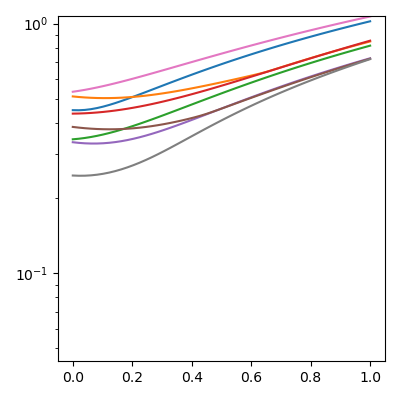
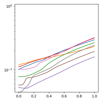
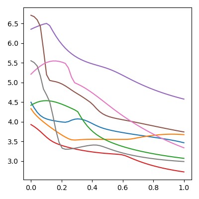
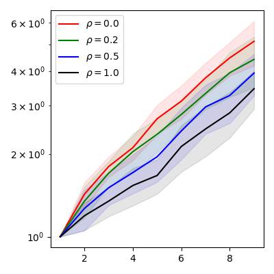
Numerical validation. To conclude the paper, we report on the results of a numerical experiment that validates our theoretical results on the singular values of deep networks and the conclusion that the loss landscape of a ResNet is more stable and less eccentric than that of a ConvNet. We constructed a toy four-layer deep network

f=f_{2}\circ f_{1}\circ f_{0}\circ f_{-1}

(158)

with $f_{k}$ of the form (1) with the nonlinear activation function $\phi_{k}$ the leaky-ReLU with $\eta=0.1$ in (35). For $f_{-1},f_{0},f_{2}$ , we set $\rho=0$ in (1), while for $f_{1}$ we let $\rho$ roam as a free parameter in the range $\rho\in[0,1]$ that includes as endpoints a ConvNet layer ( $\rho=0$ ) and a ResNet layer ( $\rho=1$ ). The input $x$ was two-dimensional, and all other inputs, outputs, and bias vectors were 6-dimensional, making the weight matrix $W_{2}$ of size $6\times 2$ and all other weight matrices of size $6\times 6$ . We generated the entries of the input $x$ , random weights $W_{k}$ , and random biases $b_{k}$ as iid zero-mean unit Gaussian random variables and tasked the network with predicting the following six statistics of $x$ by minimizing the $\ell_{2}$ norm of the prediction error (squared error):

y=\big[x[1],x[2],{\rm mean}(x),\max(x),\min(x),\|x\|_{2}\big]^{T}.

For each random $x,W_{k},b_{k}$ and each value of $\rho\in[0,1]$ , we computed the singular values of the matrix $Q$ from (50) in Lemma 8 that determine the local shape of the piecewise-quadratic loss landscape for the $0$ -th layer. We conducted 8 realizations of the above experiment and summarize our results in Figure 8.

Figure 8 not only validates the theory we have developed above, but it also enables us to draw the following concrete conclusions for gradient-based optimization of the family of DNs we have considered. Recall that the loss surface of these networks consists of pieces of (hyper) ellipsoids according to (35) in Section 3.4. Independent of the location ( $W$ ) on the ellipsoid, the more eccentric the ellipsoid, the more the gradient points away from the local optimum. Figures 8(a) and (b) indicate for increasing $\rho$ that, since the singular values increase, the image of the unit ball under $Q$ becomes wider, and thus the level sets of the local loss surface become more narrow Edelman. Moreover, Figure 8(c) and (d) show that the local loss surface becomes less eccentric as $\rho$ increases (a sphere would have a ratio equal to 1). Like our theory, these numerical results strongly recommend ResNets over ConvNets from an optimization perspective.

7 Conclusions

In this paper, we have developed new theoretical results on the perturbation of the singular values of a class of matrices relevant to the optimization of an important family of DNs. Applied to deep learning, our results show that the transition from a ConvNet to a network with skip connections (e.g., ResNet, DenseNet) leads to an increase in the size of the singular values of a local linear representation and a decrease in the condition number. For regression and classification tasks employing the classical squared-error loss function, the implications are that the piecewise-quadratic loss surface of a ResNet or DenseNet are less erratic, less eccentric and features local minima that are more accommodating to gradient-based optimization than a ConvNet. Our results are the first to provide an exact quantification of the singular values/conditioning evolution under smooth transition from a ConvNet to a network with skip connections. Our results confirm the empirical observations from li2017visualizing depicted in Figure 1.

Our results also imply that extreme values of the training data affect the optimization, an effect that is tempered when using mini-batches due to the inherent averaging that takes place. Finally, our results shed new light on the impact of different nonlinear activation functions on a DN’s singular values, regardless of its architecture. In particular, absolute value activations (such as those employed in the Scattering Network mallat2012group) do not impact the singular values governing the local loss landscape, as opposed to ReLU, which can decrease the singular values.

Our derivations have assumed both deterministic settings and random settings. In the latter, some of our results are asymptotic in the sense that the bounds hold with probability as close to 1 as desired provided that the parameters are set accordingly. We have also provided results in the pre-asymptotic regime that enable one to assess the probability that the bounds will hold.

Finally, while our application focus here has been on analyzing the loss landscape of an important family of DNs, our journey has enabled us to develop novel theoretical results that characterize the evolution of matrix singular values under a range of perturbation regimes that we hope will be of independent interest and broader use.

Acknowledgements. Richard Baraniuk was supported by NSF grants CCF-1911094, IIS-1838177, and IIS-1730574; ONR grants N00014-18-12571, N00014-20-1-2534, and N00014-20-1-2787; AFOSR grant FA9550-22-1-0060; and a Vannevar Bush Faculty Fellowship, ONR grant N00014-18-1-2047. Rudolf Riedi was supported by ONR grant N00014-20-1-2787. Thanks to Micha Wasem for stimulating discussions leading up to Lemma 21 and to Stephen Wright for pointing out the classification connection in hui21.

References

[1] R. Balestriero and R. G. Baraniuk. A spline theory of deep networks. In International Conference on Machine Learning, volume 80, pages 374–383, Jul. 2018.
[2] R. Balestriero and R. G. Baraniuk. Mad max: Affine spline insights into deep learning. Proceedings of the IEEE, 109(5):704–727, 2021.
[3] Eric Benhamou, Jamal Atif, and Rida Laraki. A short note on the operator norm upper bound for sub-Gaussian tailed random matrices. arXiv:1812.09618, 2019.
[4] Joan Bruna and Stéphane Mallat. Invariant scattering convolution networks. IEEE Transactions on Pattern Analysis and Machine Intelligence, 35(8):1872–1886, 2013.
[5] D. Chafai, O. Guedon, G. Lecue, and A. Pajor. Singular values of random matrices. In D. Chafai, editor, Lecture Notes, chapter 6, pages 147–184. Nov. 2009. djalil.chafai.net/docs/sing.pdf.
[6] Ingrid Daubechies, Ronald DeVore, Nadav Dym, Shira Faigenbaum-Golovin, Shahar Z Kovalsky, Kung-Ching Lin, Josiah Park, Guergana Petrova, and Barak Sober. Neural network approximation of refinable functions. arXiv:2107.13191, 2021.
[7] Laure Dumaz and Balint Virag. The right tail exponent of the Tracy-Widom $\beta$ distribution. Annales de l’I.H.P. Probabilités et Statistiques, 49(4):915–933, 2013.
[8] Alan Edelman. Eigenvalues and condition numbers of random matrices. SIAM J. Matrix Anal. Appl., 9(4):543–560, October 1988.
[9] Y. Gal and Z. Ghahramani. Dropout as a Bayesian approximation: Representing model uncertainty in deep learning. In International Conference on Machine Learning, pages 1050–1059, 2016.
[10] Xavier Glorot, Antoine Bordes, and Yoshua Bengio. Deep sparse rectifier neural networks. In International Conference on Artificial Intelligence and Statistics, pages 315–323, 2011.
[11] I. Goodfellow, Y. Bengio, and A. Courville. Deep Learning. MIT Press, 2016.
[12] K. He, X. Zhang, S. Ren, and J. Sun. Deep residual learning for image recognition. In IEEE Conference on Computer Vision and Pattern Recognition, pages 770–778, 2016.
[13] K. He, X. Zhang, S. Ren, and J. Sun. Identity mappings in deep residual networks. In European Conference on Computer Vision, pages 630–645, 2016.
[14] A. J. Hoffman and H. W. Wielandt. The variation of the spectrum of a normal matrix. Duke Math. J., pages 37–39, 1953.
[15] G. Huang, Z. Liu, L. Van Der Maaten, and K. Q. Weinberger. Densely connected convolutional networks. In IEEE Conference on Computer Vision and Pattern Recognition, pages 4700–4708, 2017.
[16] L. Hui and M. Belkin. Evaluation of neural architectures trained with square loss vs. cross-entropy in classification tasks. In International Conference on Learning Representations, May 2021.
[17] B. Laurent and P. Massart. Adaptive estimation of a quadratic functional by model selection. Annals of Statistics, 28(5):1302–1338, 2000.
[18] Y. LeCun and Y. Bengio. Convolutional networks for images, speech, and time-series. The Handbook of Brain Theory and Neural Networks, 3361(10), 1995.
[19] Yann LeCun, Yoshua Bengio, and Geoffrey Hinton. Deep learning. Nature, 521(7553):436–444, 2015.
[20] Hao Li, Zheng Xu, Gavin Taylor, Christoph Studer, and Tom Goldstein. Visualizing the loss landscape of neural nets. arXiv:1712.09913, 2017.
[21] Hao Li, Zheng Xu, Gavin Taylor, Christoph Studer, and Tom Goldstein. Visualizing the loss landscape of neural nets. In Advances in Neural Information Processing Systems, pages 6389–6399, 2018.
[22] S. Mallat. Group invariant scattering. Comm. Pure Appl. Math., 65(10):1331–1398, July 2012.
[23] Craig A. Tracy and Harold Widom. Level-spacing distributions and the airy kernel. Comm. Math. Phys., 159(1):151–174, 1994.
[24] Craig A. Tracy and Harold Widom. Distribution functions for largest eigenvalues and their applications. Proceedings of the International Congress of Mathematicians, I:587, 2002.
[25] Bing Xu, Naiyan Wang, Tianqi Chen, and Mu Li. Empirical evaluation of rectified activations in convolutional network. CoRR, abs/1505.00853, 2015.

largest singular value		smallest non-zero singular value
$s_{1}(\rho)=s_{1}(M_{o}+\rho\,{\rm Id})$		$s_{}(\rho)=s_{}(M_{o}+\rho\,{\rm Id})$

$\rho$		$\rho$
(a)		(b)
$\kappa(M_{o}+\rho{\rm Id})=s_{1}(\rho)/s_{*}(\rho)$		$s_{1}(\rho)/s_{i}(\rho)$

$\rho$		$i$
(c)		(d)