Generic symmetry defect set of an algebraic curve
Abstract.
Let be an -dimensional algebraic variety. We define the algebraic version of the generic symmetry defect set (Wigner caustic) of . Moreover, we compute its singularities for being a generic curve of degree in .
Key words and phrases:
symmetric defect, bifurcation points, Wigner caustic.2020 Mathematics Subject Classification
14 D 06, 14 Q 201. Introduction
Over the last two decades numerous methods have been developed to study affine geometry of surfaces and curves, especially their affinely invariant symmetry characteristics. The symmetry sets [3, 4, 5] and the center symmetry sets were investigated extensively in [11, 8, 9, 6]. Several constructions of the set equivalent to the point of central symmetry for perturbed centrally symmetric ovals were presented in the literature and resulted in the kind of symmetry defect called center symmetry set. The center symmetry set directly appears in the construction of the so-called Wigner caustic. This caustic is obtained by the stationary phase method applied to the semiclassical Wigner function which completely describes a quantum state in the symplectic phase space [2]. It is built of points where the central symmetry, i.e. the number of intervals ending in the surface and passing centrally through that point, changes. We call this set a symmetry defect or bifurcation set. In [12] this construction was generalized for algebraic varieties .
This note is motivated by the recent results of [12]. We address the problem of how to introduce a generic symmetry defect set () associated to -dimensional variety . Note that in the algebraic case we cannot use a general deformation of as it is done in the smooth case. To avoid this difficulty we will consider the linear deformation of a pair and we will study the symmetry defect set of this pair. We will show that the generic symmetry defect set is an irreducible algebraic hypersurface with nice singularities, which is defined up to the ambient homeomorphism of .
We also show:
Theorem 4.1 Let be generic plane curves of degree and , respectively, with . Then is an irreducible curve with
cusps and
nodes. It has degree, genus and Euler characteristic equal respectively to
This yields as a consequence
Corollary 4.3 Let be a generic plane curve of degree . Then is an irreducible curve of degree and genus with cusps and nodes. Moreover, .
2. Symmetry defect set
Let be a smooth manifold of dimension . For a given point we are interested in the number of pairs of points such that is the center of the interval , (mid point map). We have showed in [12] that if is an algebraic manifold in a general position, then there is a closed set such that the function is a differentiable covering outside . We call the minimal such a set the symmetry defect set of and denote it by . We have showed that the symmetry defect set is an algebraic hypersurface and consequently the function is constant and positive outside . We have estimated the number and the degree of the hypersurface
In fact we can do this in a more general setting, we can start from a pair of smooth manifolds of dimensions and respectively, where . Again, if are algebraic manifolds in a general position, then there is a closed set such that the function is a differentiable covering outside . The minimal such a set is an algebraic hypersurface which we call the symmetry defect set of and and denote it by .
However, in general the hypersurface (or ) has bad singularities. In this paper we will introduce the stable (generic) versions of and . To do this we cannot use general deformation of as in the smooth case. In fact we can use here only linear deformations, but this is not enough to obtain a stable . The good solution is to consider the pair and to deform this pair.
Definition 2.1.
Let be a smooth manifold. We will say that the hypersurface has Thom-Boardman singularities, if there is a smooth manifold and a Thom-Boardman mapping such that is a discriminant of .
We have:
Theorem 2.2.
Let (where ) be smooth algebraic manifolds and let denote the group of affine linear automorphisms of . There is a Zariski open subset such that for every the hypersurface has only Thom-Boardman singularities. Moreover, if and then the hypersurfaces and are ambient homeomorphic.
Proof.
Let us consider the variety Consider the general projection By Mather’s theorem (see [15] and [7]) there is an Zariski open subset such that if then the projection is transversal to the Thom-Boardman strata. Moreover by [13] we can shrink such that all projections are topologically equivalent. Now consider the map (here ). Now it is enough to take ∎
Definition 2.3.
Let be smooth algebraic manifolds. By the generic symmetry defect set we mean the set where are sufficiently general. We denote it by . This set is defined up to the ambient homeomorphism. We write .
Remark 2.4.
Of course we can take here to be identity and take the map as close to the identity as we wish.
We show in Section 3 that if neither nor is a linear space then is an irreducible hypersurface with Thom-Boardman singularities. In particular in the case the curve has only cusps and nodes as singularities and the number of these cusps and nodes is an affine invariant of and . In Section 4 we compute these numbers for generic plane curves and of degrees and , respectively.
3. The set is irreducible
We need the following theorem concerning the properties of linear systems on algebraic varieties, due to E. Bertini [1]:
Theorem 3.1.
Let be an algebraic variety over an algebraically closed field of characteristic , let be a linear system without fixed components on and let be the image of the variety under the mapping given by . Then:
(1) If dim then almost all the divisors of the linear system (i.e. all except a closed proper subset in the parameter space ) are irreducible reduced algebraic varieties.
(2) Almost all divisors of have no singular points outside the basis points of the linear system and the singular points of the variety .
Let us recall that if we have a projective hypersurface then we have the dual map and the variety is called the dual to . More generally if is of arbitrary dimension and then the hyperplane is tangent to if is contained in (here we consider as a projective subspace of ). We have a well-known reflexivity property: . From this it easily follows that:
Proposition 3.2.
Let be a hypersurface in If then is ruled, i.e., through every point there is a projective linear subspace of dimension .
Now we can pass to the main result of this section:
Theorem 3.3.
Let be a smooth algebraic variety of dimension . Assume that is not ruled. Then the critical set and the discriminant of a generic projection are irreducible. Moreover, is smooth and has only Thom-Boardman singularities.
Proof.
We can write where and are generic projection. By Mather’s Theorem (see [15]) the variety has only normal crossings outside critical values of . Since the set of critical values has codimension two or more we can assume that has only normal crossings. Let be all irreducible components of . Take sufficiently general points . Then two different branches of meet in , in particular we have two different tangent spaces and to these branches. The set of projections which induce isomorphisms on all spaces is open and dense in the family of such projections .
Hence in fact we may prove our theorem only for and a generic projection . We apply here Theorem 3.1. Note that the critical set of a projection given by equations is described by an equation:
| (3.1) |
where is the equation of and
Note that if goes through all possible projections then (3.1) forms a linear system on . Of course it has no base points on . It is enough to prove that . First note that if and is not parallel to then there is a section of such that and . Indeed, it is enough to take a projection with center such that but and the section given by . Hence separates points with not parallel tangent spaces. Now we need the following:
Lemma 3.4.
Let be an irreducible subvariety such that for all the tangent spaces are parallel. Then there is a hyperplane such that and for every .
Proof.
We may assume that is not a point. Assume that all tangent spaces , are parallel to some hyperplane given by equation . If then for we have and all tangent spaces are equal to . If , then by Sard’s theorem there is a such that the hyperplane is transversal to , a contradiction. ∎
Now assume that is a component of a fiber of the mapping . Then all tangent planes , are parallel. From Lemma 3.4 we have that for some hyperplane and every . In particular is in the fiber of the mapping . Since is not ruled and is a linear birational projection of , the variety is also not ruled. In particular general fibers of the mapping have dimension less than . Hence dim .
The last statements follows from Mather’s projection theorem. ∎
Remark 3.5.
The assumption that is not ruled is essential. Indeed, every generic projection of a cylinder to has reducible critical set and reducible discriminant.
Corollary 3.6.
Let be a smooth algebraic varieties. If neither nor is linear then the set is an irreducible hypersurface.
Proof.
If and are not linear then they are ruled in dimension at most . Hence is ruled in dimension at most and we can apply Theorem 3.3. ∎
4. for generic plane curves ,
Theorem 4.1.
Let be generic plane curves of degree and , respectively, with . Then is an irreducible curve with
cusps and
nodes. It has degree, genus and Euler characteristic equal respectively to
Proof.
To make the proof easier to read we will divide it into five steps.
Step 1: Basic definitions and construction of .
Let and where and are a general polynomials of degree and , respectively. We will consider . We denote the coordinates in by and the coordinates in by (slightly abusing notation). We denote the partial derivative by a lower index, e.g. . By we denote the homogenization of with respect to and by we denote the dehomogenization of with respect to . Note that in we first take the partial derivative and then the homogenization and dehomogenization. We will also denote the projective closure of a variety by .
Since is generic and has degree , there are distinct points of intersection of with the line at infinity, say , for . Similarly, let , , be the points of intersection of with the line at infinity. Let and be the corresponding points in . Note that the lines spanned by and also lie in . Since is a surface of degree , the intersection of with the hyperplane at infinity consists only of those lines.
Now consider a generic projection Composing with a linear change of coordinates in the target we can assume that , where are generic. Let
| (4.1) |
Let denote the critical set of . It is given by equations:
| (4.2) |
We denote by the curve .
Since is generic, the values , , and are nonzero. Thus, for a generic choice of we obtain
for some nonzero constants . This means that the hypersurface defined by intersects the lines spanned by and only at the points and . It follows that is a complete intersection given by , at least set-theoretically.
Step 2: Examining the branches of at infinity.
Now we will focus on examining the branches of at infinity. Without loss of generality we may examine only branches through and assume that . We will work in the neighborhood defined in by . The notation means here a series in of order strictly larger than .
We can write down up to multiplying by a constant as
where is the homogeneous part of of degree . Here we work in and omit the and variables as they do not occur in . Let
We claim that for a suitable series in the function vanishes on the curve parametrized for small by for . Indeed, we have and we may continue the process of defining up to in such a manner that , passing with to infinity we obtain that . Namely, if and then setting we obtain .
Now we will construct and , for , so that
parametrizes for small a curve in the zero locus of . Take and . We have
thus we need to ensure that . Furthermore,
thus we need to ensure that , where and are constants dependent on and the homogeneous part of of degree . So we have to take and such that the point lies in the intersection of curves given in by and . Moreover, we are able to expand and up to degree in such manner that and . Indeed, if we expand and up to degree then we can obtain the coefficients of by solving a system of two linear equations with two variables. The determinant of the matrix associated with the system is
which is nonzero for generic . Thus the system of equations has a unique solution.
To make sure that we indeed obtain distinct curve germs we need to use the genericity of , and to ensure that has distinct solutions. To abbreviate the argument we will say in this case that is good. For any fixed pair there is a dense subset of , the product of spaces of bivariate polynomials of degree, respectively, at most or , such that is good. This implies, that the set of good is dense in . It is also constructible, so it contains an open dense subset. In particular, for generic and there is an open dense subset such that for all the quadruple is good. The values and depend only on and for generic they are nonzero, i.e., does not intersect nor at infinity. Thus for generic the pair is in .
Summarizing, has points of at infinity: for and for . At each of the curve has distinct branches. By symmetry at each of the curve has distinct branches. Thus has branches at infinity. In particular is a scheme-theoretic complete intersection of , and . Moreover, is a curve of degree and, consequently, is a curve of degree as well.
Step 3: Computing the number of cusps of .
Note that each cusp of is the image of a unique critical point of . Thus , the number of cusps, is equal to the number of points of at which the matrix
| (4.3) |
fails to have maximal rank. Since , and don’t have common zeroes, the second row of does not vanish on . Moreover, vanishes on , so the first, second, fourth and fifth row of are linearly dependent. It follows that the rank of does not decrease after removing the first row. We denote the determinant of without the first row by , i.e.,
Now we compute the intersection multiplicity of the zero locus of with at and . For it suffices to determine the order of for the branches of at . Recall that
thus , , and composed with have order and and composed with have order . By genericity of and the initial coefficient does not vanish, so the order of is . The computation will not be fully symmetric for . A branch at a point will have the form
Thus, after composing with , and will have order , and will have order and and will have order . So the order of is . Summing up we obtain that the intersection multiplicity is at points and at points .
Note that and intersect transversally because otherwise would have a singularity other than a cusp or a node. Thus by Bezout’s Theorem the number of intersection points is
Step 4: Computing the Euler characteristic and genus.
Note that the mapping is a ramified covering of degree , with the discriminant . Let denote the number of nodes of and denote the number of cusps. Let us recall that the mapping is generically one-to-one and the fiber has more than one point (in fact then it has exactly two points) only if is a node. Consequently we can write the following equality:
The equation simplifies to:
| (4.4) |
Moreover we have , so . Similarly, . Furthermore, , so . Substituting these equalities to equation (4.4) we obtain:
From the equality we obtain:
Step 5: Computing the number of nodes of .
We will use the following theorem of Serre (see [17], p. 85):
Theorem 4.2.
If is an irreducible curve of degree and genus in the complex projective plane then
where denotes the delta invariant of a point .
In order to use this Theorem we will need to compute the delta invariants of points at infinity of . Note that if is a branch of at , then will be a branch of at . If is a branch of at then will be a branch of at . Thus for generic projection , i.e. generic quadruple , the curves and will have the same number of distinct points at infinity.
Now we will show, that the branches at infinity of are pairwise transversal. By symmetry it is enough to show this for branches at . Consider a branch for small but nonzero. In the projective space we have
thus in the space in which was originally defined we have
Consequently,
In the projective space we have
Thus a branch of at is parametrized by , so is a tangent vector at . Since the points are distinct we conclude that for a generic quadruple we have for . So distinct branches have distinct tangent spaces.
Since has pairwise transversal branches at we obtain . Similarly, .
By the Serre formula we have
The only unknown value in this equation is the number of nodes. After simplification we obtain
∎
Taking in Theorem 4.1 we immediately obtain:
Corollary 4.3.
Let be a generic plane curve of degree . Then is an irreducible curve of degree and genus with cusps and nodes. Moreover,
In particular for we have:
Corollary 4.4.
Let Then is an irreducible elliptic curve with cusps and nodes.
Note that neither nor satisfy the conditions of genericity imposed in the proof of Theorem 4.1, however a generic curve of degree can be reduced to and via affine transformations.
In the real case we have a finite number of possible and for the real circle and the real hyperbola . As an example we present in Figure 1 the images of and for and .
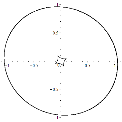
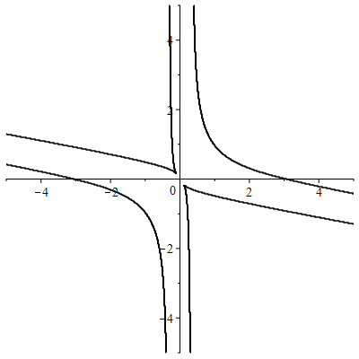
The real curve has four cusps and the real curve has two cusps.
Acknowledgment. All authors were partially supported by the grant of Narodowe Centrum Nauki number 2019/33/B/ST1/00755. The authors are grateful to professor M.A.S. Ruas for many helpful discussions.
References
- [1] Y. Akizuki, Theorems of Bertini on linear systems, J. Math. Soc. Japan 3, (1951), 170–180.
- [2] M. Berry, Semi-classical mechanics in phase space: A study of Wigner’s function, Phil. Trans. Roy. Soc. 287 (1977), 237–271.
- [3] J.W. Bruce, P.J. Giblin, C.G. Gibson, Symmetry sets, Proc. Roy. Soc. Edinburgh 101A, (1983), 163–186.
- [4] J. Damon, Smoothness and geometry of boundaries associated to skeletal structures I: Sufficient conditions for smoothness, Ann. Inst. Fourier, Grenoble, 53, 6 (2003), 1941–1985.
- [5] J. Damon, Determining the Geometry of Boundaries of Objects from Medial Data, International Journal of Computer Vision 63(1), (2005), 45–64.
- [6] W. Domitrz, P. Rios, Singularities of equidistants and global centre symmetry sets of Lagrangian submanifolds, Geom. Dedicata 169, (2014), 361–382.
- [7] M. Farnik, Z. Jelonek, M.A.S. Ruas, Whitney theorem for complex polynomial mappings, Math. Z. 295 (2020), 1039–1065.
- [8] P.J.Giblin, P.A.Holtom, The centre symmetry set, Geometry and Topology of Caustics, Banach Center Publications Vol. 50, ed. S. Janeczko and V.M. Zakalyukin, Warsaw, 1999, 91–105.
- [9] P.J. Giblin, S. Janeczko, Geometry of curves and surfaces through the contact map, Topol. Appl. 159 (2012), 379–380.
- [10] R. Hartshorne, Algebraic Geometry, Springer Verlag, New York, 1987.
- [11] S. Janeczko, Bifurcations of the Center of Symmetry, Geom. Dedicata 60, (1996), 9–16.
- [12] S. Janeczko, Z. Jelonek, M.A.S. Ruas, Symmetry defect of algebraic varieties, Asian J. Math. 18, (2014), 525–544.
- [13] Z. Jelonek, On semi-equivalence of generically-finite polynomial mappings, Math. Z. 283, (2016), 133–142.
- [14] S. Kleiman, The enumerative theory of singularities, Real and complex singularities – Proc. Ninth Nordic Summer School NAVF Sympos. Math., Oslo (1976), 297–396.
- [15] J.N. Mather, Generic projections, Ann. of Math. (2) 98, (1973), 226–245.
- [16] J.N. Mather, On Thom-Boardman singularities, Dynamical Systems Proceedings of a Symposium Held at the University of Bahia, Salvador, Brasil, July 26-August 14, 1971, (1973), 233–248.
- [17] J. Milnor, Singular points of complex hypersurfaces, Annals of Mathematics Studies, Princeton University Press, (1968).