Geometric Hermite Interpolation in by Refinements
Abstract
We describe a general approach for constructing a broad class of operators approximating high-dimensional curves based on geometric Hermite data. The geometric Hermite data consists of point samples and their associated tangent vectors of unit length. Extending the classical Hermite interpolation of functions, this geometric Hermite problem has become popular in recent years and has ignited a series of solutions in the 2D plane and 3D space. Here, we present a method for approximating curves, which is valid in any dimension. A basic building block of our approach is a Hermite average, a notion introduced in this paper. We provide an example of such an average and show, via an illustrative interpolating subdivision scheme, how the limits of the subdivision scheme inherit geometric properties of the average. Finally, we prove the convergence of this subdivision scheme, whose limit interpolates the geometric Hermite data and approximates the sampled curve. We conclude the paper with various numerical examples that elucidate the advantages of our approach.
Keywords: Hermite interpolation, curve approximation, nonlinear averaging, subdivision schemes.
MSC2020: 65D05, 65D10, 53A04, 65Y99.
1 Introduction
The problem of geometric Hermite approximation is to estimate a curve from a finite number of its samples, consisting of both points on the curve and their associated, normalized tangent vectors. This problem is fundamental in Computer Aided Geometric Design (CAGD), see, e.g., [7, 25, 36], but it also appears in various other applied topics such as biomechanical engineering [4], marine biology [34], scientific simulations [35], CNC machining [2] and more. The primary challenge in geometric Hermite approximation is to incorporate the additional information, given in the form of normalized tangent vectors, for obtaining a better approximation of the sampled curve than approximation based on points only. Moreover, the fact that the curve lies in a high-dimensional space poses additional practical and theoretical difficulties. Our approach provides a unified solution that copes with the above, and generates approximation with many favorable geometric properties.
Classical Hermite interpolation deals with the linear problem of interpolating a function to data consisting of its values and its derivatives’ values at a finite number of points by a polynomial. In [26], a family of linear Hermite subdivision schemes is introduced. This work opened the door for solving Hermite-type approximation through refinement [9, 12, 16, 18, 27]. Although all these subdivision schemes are linear, refinement is the approach taken in this paper to the nonlinear problem of geometric Hermite interpolation.
Recent years have given rise to many nonlinear subdivision schemes and, in particular, to operators refining 2D and 3D geometric Hermite data, e.g., [1, 23, 31]. The design of such subdivision operators is typically based on the reconstruction of geometric objects from a certain class. Such operators were suggested for circle reconstruction [3, 23, 32], ellipse reconstruction [5], local shape-preserving [6, 24] and local fitting of clothoids [31]. The relative simplicity and high flexibility in the design of refinement rules allow posing advanced solutions for modern instances of the Hermite problem, e.g., for manifold values [28, 29]. The latter is an example of the agility of subdivision schemes, perhaps best illustrated when considering the variety of methods that serve as approximation operators over diverse nonlinear settings. Note that although the Euclidean space is linear, the problem of geometric Hermite approximation for data sampled from a curve in an Euclidean space is nonlinear. This is due to the fact that the space of pairs of point-normalized tangent (for short, point-ntangent) is not linear, as it is a subset of .
In our approach, we interpret the refinement rules of a subdivision scheme as a method of averaging, as in [10, 14, 33]. Thus, generating curves in a nonlinear environment boils down to properly defining and understanding the averaging in the particular space. While most of the work in this direction refers to non-Hermite problems, some recent papers such as [22, 23, 31] introduce different techniques for averaging two point-normal pairs in the plane. Therefore, as a first step, we formulate the notion of Hermite average in , which encapsulates the concept of averaging two point-ntangent pairs sampled from a curve in for any . We then propose a nonlinear average in that is based on Bézier curves and satisfies the requirements of the Hermite average. Determining such a mean is crucial for constructing our subdivision operators. Our paper is an example of how the averaging approach can serve as a fundamental bridge for obtaining approximation operators in general metric spaces, see also, e.g., [19].
The construction of our approximation operators, begins with the study of our Hermite average termed hereafter Bézier average. We show that this average satisfies several geometric properties such as invariance under similarity transformations and preservation of lines and circles. Then, we form a two-point interpolatory subdivision scheme by repeatedly applying the Bézier average as an insertion rule. This subdivision scheme serves as an illustrative example, which demonstrates the benefits of using our approach for constructing approximation operators based on refinement. For example, the geometric subdivision scheme we form inherits the geometric properties of the Bézier average; it is invariant under similarity transformations, it reconstructs lines and circles. Furthermore, our general approach of using an appropriate average, enables us to obtain a large class of nonlinear subdivision schemes refining geometric Hermite data, by replacing the linear average in the Lane–Riesenfeld subdivision schemes [20] by the Bézier average.
As part of the analysis, we prove the convergence of our interpolatory subdivision scheme, namely that it refines geometric Hermite data and its limit is a smooth curve that interpolates both the data points and their normalized tangent vectors. Moreover, the limit normalized tangent vectors are tangent to the limit curve. The proof of convergence of our non-linear subdivision scheme uses an auxiliary result which we validate with computer-aided evidence, combining analysis of multivariate functions and exhaustive search done by a computer program. The details appear in Appendix A and as a complementary software code.
One additional advantage of our method is that the new schemes based on the Bézier average, allow us to use a more flexible sampling strategy than typically assumed when applying subdivision schemes to approximate curves from Hermite data [15]. We demonstrate this property numerically, emphasizing the approximation capabilities and how it assists in avoiding geometric artifacts, see Section 4. In addition, we present numerical evidence of fourth-order approximation of curves, which is higher than what current theory guarantees for non-uniform sampling [15]. This fourth-order approximation of curves generalizes similar results in classical Hermite interpolation of functions. We also compare numerically our schemes with other known methods and illustrate the superiority of techniques based on the Bézier average. The entire set of examples is available for reproducibility as open Python code in https://github.com/HofitVardi/Hermite-Interpolation.
The paper is organized as follows. Section 2 presents the precise statement of the fundamental approximation problem we solve and defines the notion of Hermite averaging. Then, we introduce our Bézier average and prove that it is Hermite average. The section is concluded with several geometric properties of this new Hermite average. Section 3 shows how to form Hermite subdivision schemes based on the Bézier average. There we offer additional properties of the Bézier average and use them to prove the convergence of our interpolatory Hermite subdivision scheme. In Section 4 we explore our solution to the problem of geometric Hermite interpolation numerically. The numerical examples demonstrate the performance of our Hermite subdivision schemes compared to other approximants. In the last section, conclusions and future work are discussed. This paper is accompanied by three appendices that include the computer-aided evidence mentioned above, proofs of some claims from the main sections, and a further discussion on the Bézier average.
2 Averaging in the Hermite setting
It is important to place the motivation behind the following discussion in the area of Hermite approximation. We thus begin with some essential notation and definitions, leading to the formulation of the problem of geometric Hermite interpolation.
In the following subsections we state a few lemmas and a proposition. The proofs of these results are given in Appendix B.
2.1 Notation and definitions
A geometric Hermite data is a sequence
| (2.1) |
where is the Euclidean dimensional space equipped with the Euclidean metric, is the sphere equipped with the angular metric, and where . We view such a sequence as samples of a curve, consisting of points and tangent directions. Unless otherwise stated, we denote by and the Euclidean and angular metrics on and , respectively. Moreover, and refer to the Euclidean inner product and norm in .
Let s.t. .
Consider the following functions of :
The normalized vector of difference between and is
| (2.2) |
The distance between and in terms of their angular distance is
| (2.3) |
The deviations of and from (in terms of their angular distance) is
| (2.4) |
The norm of , regarded as a vector in , is
| (2.5) |
The last quantity was first used in [31] in the convergence analysis of a Hermite subdivision scheme.
When there is no possibility of ambiguity, we omit the notation of the variables and simply write and .
We conclude with the definition of the problem we solve.
Definition 2.1.
The problem of geometric Hermite interpolation is to find a curve which interpolates the geometric Hermite data , see (2.1), where . We assume the data is sampled from a curve ,
| (2.6) |
with for all . Here operates on curves and returns the ntangent to a curve at a specified parameter value. The curve should satisfy the interpolation conditions,
| (2.7) |
where is a parametrization and for all .
2.2 Hermite Average
We address the problem of geometric Hermite interpolation through a subdivision process which is defined via an average over . We call this average a Hermite average, define it, and later propose a method to construct such a mean. The new definition illustrates some of the significant differences between classical and geometric Hermite settings.
The classical concept of average is perhaps best demonstrated by the case of positive real numbers, see ,e.g., [17]. An average is a bivariate function with a weight parameter
For brevity, we use the form where is the weight. It is worth noting that in some cases it is essential to extend the weight parameter beyond the segment, see e.g., [13]. The popular value leads to the well-known average expressions such as or , that correspond to the linear and geometric averages. Many other common families of averages exist, for example the -averages , which include the above linear and geometric means as special cases. This example is itself a special case of a wider family of averages of the form , when is an appropriate invertible function. The -averages family comes up when using . For more details, see [10].
As we generalize the concept of averaging to more intricate settings, we wish to follow the averages’ fundamental properties. Namely, the basic properties satisfied by the above bivariate function ,
- 1.
Identity on the diagonal: .
- 2.
Symmetry: .
- 3.
End points interpolation: and .
- 4.
Boundedness: .
Note that the last property, unlike the first three, requires ordering (partial ordering). This harsh requirement can be relaxed by using a metric and modifying the last property to ensure metric-related boundedness.
Considering the classical case and the absence of a “natural” metric in the Hermite setting, we define a Hermite average by adjusting the first three properties listed above. Recall that a pair of elements in our domain is viewed as two samples of a regular, differentiable curve. Thus, there is a native hierarchy associated with the direction of the curve. Under this interpretation, it makes sense to consider an average that is sensitive to orientation. It also calls for a different understanding of the diagonal since an element cannot represent two distinct, yet close enough samples of a regular curve. Therefore, we refer to the diagonal utilizing the notion of limit. The limit we consider is the most fundamental approximation as one approaches a point on a curve. Finally, we treat the symmetry as reversing the curve and so the orientation of the points. Next is the formal definition.
Definition 2.2.
We term a Hermite average over if and the following holds for any and ,
- 1.
Identity on the “limit diagonal”:
- 2.
Symmetry with respect to orientation:
- 3.
End points interpolation:
Remark 2.3.
In the presence of an appropriate metric , the classical boundedness property can emerge as
where
2.3 Bézier Average
In this section we introduce the “Bézier average”. While the definition considers a weighted average for any weight , we mainly focus on the special case , which is required for our refinements.
We start our construction with an admissible pair that satisfies the following two conditions
| (2.8) |
where is defined in (2.2).
The full reasoning behind the conditions of (2.8) is revealed in the following discussion. Our next step is to generate the Bézier curve, which we denote by , based on the following control points:
| (2.9) |
Here,
| (2.10) |
and are as defined in (2.4). Note that the second condition of (2.8) guarantees that (2.10) is well-defined since .
The Bézier curve is given explicitly by
| (2.11) |
and its derivative is thus,
| (2.12) |
Remark 2.4.
Note that if are linearly independent as vectors in then for any . Moreover, it can be shown that if two of those vectors are linearly dependent while the third is independent of each one of them, then for any . As well, it can be verified that if then .
We are now ready to present the Bézier average.
Definition 2.5.
The Bézier average of and with weight is defined as the point and its normalized tangent vector of the Bézier curve (2.11) at . Namely,
| (2.13) |
where and (or if ).
In the spirit of Definition 2.1, the above means that if of (2.11) is a regular curve, that is does not vanish, then for any .
Figure 1 demonstrates the procedure of averaging according to Definition 2.5. In particular, we present two examples that correspond to two different cases. On the left the Bézier curve which we sample according to Definition 2.5 is convex, while on the right it is non-convex.
Definition 2.5 does not guarantee that the tangent vector is non-vanishing. That is to say, one can find examples of two pairs of Hermite data where . However, as is stated in the next lemma, this is not the case for .
Lemma 2.6.
Next we claim that the Bézier average (Definition 2.2) is a Hermite average over (Definition 2.5). For the Bézier average we define to be the set of all pairs in satisfying conditions (2.8) and producing non vanishing averaged vectors for any weight in . Note that by Remark 2.4 is not empty. A discussion about the set is differed to Appendix C.
Proposition 2.7.
The Bézier average is a Hermite average over .
Remark 2.8.
The value of we chose for the definition of the Bézier average, is suggested in [4] in order to approximate circular arcs in by Bézier curves. In case and under certain assumptions about the input, this choice coincides with the choice of . The latter choice of yields the average defined in [22], which can also be shown to be a Hermite average over a suitable set.
2.4 Geometric properties of the Bézier average
We conclude this section by introducing three additional properties of the Bézier average, which are of great value in the context of generating curves. The first property shows that averaging two point-ntangent pairs is invariant under similarities appropriate for Hermite data. This essential property of the Bézier average follows from the invariance of Bézier curves under affine transformation.
Lemma 2.9 (Similarity invariance).
The Bézier average is invariant under similarities in the following sense:
- 1.
The Bézier average is invariant under isometries applied to both and . That is, given an isometry ,
(2.16) where .
- 2.
The Bézier average is invariant under scaling: if , for any , then,
(2.17)
The following two results show two important geometric properties of the average.
Lemma 2.10 (Lines preservation).
Let be two geometric Hermite samples from a straight line, . Then, the Bézier average coincides with the linear average of each component, namely,
| (2.18) |
Note that the average in (2.18) is a point-ntangent pair from the line .
Lemma 2.11 (Circles preservation).
Assume are samples of a circle and its ntangents. Then, their average at consists of the mid-point and its ntangent of the circle-arc, defined by , and , .
3 Subdivision schemes based on the Bézier Average
In the previous section we describe the concept of Hermite average and introduce such an average — the Bézier Average. We also present some of the main properties of the Bézier average. This essential building block is the first step in constructing curves’ approximations. The next step is to use an approximation operator, which can be defined in terms of binary averages, and replace the binary average by a Hermite average. As approximation operators, we use subdivision schemes, which enjoy simple implementation and are used extensively for modeling, approximation, and multiscale representations of curves.
As an illustrative method, the main subdivision scheme we utilize is the interpolatory two-point scheme. This simple method demonstrates the application of the Bézier average and how the average’s properties are inherited by the approximation process. We define the new refinement rules and prove the convergence of this subdivision scheme for any initial admissible data.
3.1 From Hermite average to Hermite subdivision schemes
We start with the following lemma, which, together with Lemma 2.6, asserts that the process of midpoint averaging can be performed repeatedly.
Lemma 3.1.
Lemma 3.1 allows us to design a Hermite interpolatory subdivision scheme utilizing the Bézier average with as an insertion rule. Namely, for initial Hermite data of the form , , we define for all :
| (3.1) |
We refer to the subdivision scheme (3.1) as the interpolatory Hermite-Bézier scheme, in short IHB-scheme.
We view the IHB scheme as a modification of the piecewise linear subdivision scheme, which is also known as Lane-Riesenfeld of order subdivision scheme (LR1). This scheme serves as an illustrating example for our general method where we replace the linear average in any LR scheme of order , by the Bézier average with . The modified scheme refines Hermite data and we term it Hermite-Bézier Lane-Riesenfeld of order (HB-LRm). The refinement step of this scheme is given in Algorithm 1.
For the HB-LRm scheme with , we obtain a subdivision scheme which is not interpolatory, namely, the interpolation conditions (2.7) are not fulfilled. However, we expect the HB-LRm schemes to approximate the curve, as seen visually in the numerical examples in Section 4.
As a first demonstration, we show the repeated refinements of two elements in by the IHB-scheme, as appear on Figure 2 and Figure 3 for and , respectively. These figures visually reveal some properties, in particular convergence of the IHB scheme, which we present and show in the sequel.
Next, we present geometric properties of the HB-LRm schemes with which are a direct consequence of geomeric properties of the Bézier average, as given in Lemma 2.9, Lemma 2.10, and Lemma 2.11. In particular, the first part of the following result shows that preservation of geometric objects by the average becomes reconstruction of these objects by the modified subdivision schemes.
Theorem 3.2.
The HB-LRm schemes of order reconstruct lines and circles. For converging HB-LRm schemes, their limits are invariant under isometries and scaling transformations.
From here and until the end of this section, we focus our attention on the IHB-scheme (HB-LR1). Next, we present auxiliary results on the Bézier average and then present the convergence analysis of the IHB-scheme.
3.2 Contractivity of the Bézier Average
Let be given. As in the previous section, we always assume that and we denote by and the point and vector obtained by the Bézier average with weight applied to the given data. The following two lemmas play a central role in the convergence analysis of the IHB-scheme.
Lemma 3.3.
If then .
Furthermore, if then there exists such that .
Lemma 3.4.
If . Then,
We do not provide a formal proof of Lemma 3.4. Instead, we give in Appendix A a comprehensive discussion where we show that proving the lemma is equivalent to showing the positivity of an explicit trigonometric function. Then, we introduce numerical indications for the positivity of this function and an outline for a proof based on a further exhaustive computer search.
Remark 3.5.
The above two lemmas shed light on our exploration of a natural metric; see, e.g., Remark 2.3. On the one hand, Lemma 3.3 guarantees the boundedness of the Euclidean metric over a subset of . On the other hand, even though is not a metric over , it gives a measure of how far an ordered couple of point-vector pairs is from being sampled from a line. It is the result of Lemma 3.4 that the Bézier average yields two pairs that are “closer” to samples from a line than the original pair.
3.3 G1 Convergence of the IHB-scheme
First, we recall several definitions and notation needed in the convergence analysis. Initial control points is a sequence of points in . A subdivision scheme refining points refines and generate the control points , . Associating the point with the parameter value , we define at each level the piecewise linear interpolant to the points , (also known as the control polygon at level ). With these notions we can define the convergence of We term convergent if the sequence converges uniformly in the norm. In addition, we follow the definition given in [11] regarding G1 convergence of a subdivision scheme refining points, and say that is G1 convergent if it is convergent and there exists a continuously varying directed tangent along its limit curve.
A Hermite subdivision scheme is termed convergent if it is convergent as a points refining scheme and is convergent as tangents refining scheme such that the limit tangents are tangent to the limit curve, see e.g., [11, 22, 31]. Note that the normalized tangents are points on the sphere, and that the definition of convergence can be generalized to manifold-valued data if instead of piecewise linear interpolants we use piecewise geodesic interpolants (see Definition 3.5. in [14]).
By Theorem 3.6. in [14], sufficient conditions for a subdivision scheme refining points to be convergent are displacementsafe and a contractivity factor . The first requires a bound between two control polygons of consecutive refinement levels, and it trivially holds for interpolatory schemes. The second one means that
Back to the Hermite setting, with the initial data and with the refined Hermite data at the -th refinement level, and its associated
| (3.2) |
In addition, we define the piecewise geodesic interpolant of the tangent vectors at the -th refinement level as
| (3.3) |
where is the sphere geodesic average, namely is the unique point on the great circle connecting two non-antipodal points and , that divides the geodesic distance between and in a ratio of when measuring from and when measuring from . Then, we conclude:
Theorem 3.6.
The IHB-scheme is convergent whenever the initial data satisfies .
Proof.
Let be the initial Hermite type data with . We begin with the convergence of the ntangents. To this end, we prove that is a Cauchy series for all . The proof follows closely the proof of Theorem 3.6. in [14].
Recall of (2.3) and and as defined in (2.4). Then, we observe that for any ,
Let , . Then, is bounded by
with . The last inequality follows from Lemma 3.4. Thus converges uniformly and the IHB-scheme is convergent as a refining scheme of ntangents.
We now consider the IHB-scheme as a point refining scheme. It is interpolatory and hence displacement-safe. To derive a contractivity factor we consider levels with large enough, such that , where for . By Lemma 3.3,
with in the proof of Lemma 3.3. It follows that the IHB-scheme has a contractivity factor of as a point refining scheme, and thus we deduce the convergence of the points.
Finally we observe that since both the angles between to and to approaches zero when approaches infinity. This means that the limit tangents are tangent to the limit curve.
We conclude that the IHB-scheme is G1 for data satisfying . ∎
Remark 3.7.
4 Numerical examples
This section provides 2D and 3D examples of interpolating or approximating curves based on geometric Hermite samples. Specifically, we test the performance of the IHB-scheme and the HB-LR3 scheme (modification, based on the Bézier average, of the LR3 algorithm). We then compare these results to approximations by related methods, such as other modifications of LR1, see Remark 3.7.
Note that all the examples of this section are available as Python code for reproducibility and for providing a further point of view, in https://github.com/HofitVardi/Hermite-Interpolation.
4.1 Comparison between different modifications of LR1
In the first example, we compare the IHB-scheme with the modification of LR1 in [22]; see also Remark 2.8 and Remark 3.7. We apply both schemes to data sampled from spirals in and .
Figure 4 shows the limit curves obtained from samples with increasing density. As demonstrated in the figure, for a high density of samples, the performances of the two schemes are almost identical. However, as the number of samples decreases, the performance of the IHB-scheme is superior. Note that as mentioned in Remark 2.8, in the 2D case and for a sufficiently dense sampling, the two methods coincide. This example indicates similar behavior in 3D.
4.2 Geometric versus linear Hermite interpolation
We interpolate geometric Hermite data, sampling the curve , by the IHB-scheme and by a linear Hermite subdivision scheme. The latter subdivision was introduced in [26], and we term it Merrien-scheme. The Merrien-scheme is based on cubic Hermite interpolation, and uses point-tangent pairs with tangents that are not normalized as its initial data. Nevertheless, from the reasoning we present next, we compare the above two schemes when applied to geometric Hermite data, with different sampling rates.
For approximating a function by subdivision schemes, we assume that the points where we sample the function are equidistant. For curves approximation, the samples have to be close to equidistant with respect to the arc-length parameterization, see, e.g., [15]. To imitate such an ideal sampling in the Hermite setting, one must consider the distance between the points and the tangents’ magnitude. Therefore, to show the effect of sampling, we fix the tangents to be normalized and apply different sampling rates in the current comparison.
Figure 5 demonstrates the way linear Merrien-scheme and the IHB-scheme address sparse sampling (top and middle left sub-figures) and dense one (bottom sub-figure). We observe that the sampling rate significantly affects the approximation quality of the linear scheme. In particular, sparse samples yield a “flattened” curve, and dense samples generate unnecessary loops. On the other hand, the Bézier average, being adaptive to the distance between the two points, provides a remedy.
4.3 The contribution of the tangent directions to the approximation
In the following example, we test the contribution of the tangent directions to the quality of the approximation. This contribution is clear when sampling a periodic curve in parameter distances which are equal to its period. In this case, the only reasonable approximation in the absence of tangent directions is a straight line. On the other hand, our scheme when applied to Hermite data sampled from the curve , in parameter distances which are equal to its period, preserves the oscillations of (see the first sub-figure of Figure 6). Note that this cannot be the case when the sampled points are extremum points.
We demonstrate the contribution of the tangent directions in two ways: How well information about the initial tangent directions affects the quality of the approximation and how the Hermite setting can be effective even in the absence of information on the initial tangent directions.
We compare the HB-LR3 scheme, as discussed in Section 3.1, with the linear LR3 scheme. We do so by applying the HB-LR3 once to real Hermite data sampled from , and once to Hermite data, obtained from data consisting of points only, by an algorithm which estimate a tangent direction at a point using the point and its immediate neighboring points; see, e.g. [37] and Remark 4.1 below.
The results of our experiments are presented in Figure 6 and indicate the clear superiority of the approximation based on the right tangent directions. Moreover, in the absence of such information, the HB-LR3 scheme still produces a better approximation than the linear LR3 scheme, which in some cases fails to describe the curve under the limited available data. Note that this comparison follows a similar experiment done in [23] and also indicates the limitation in estimating the tangent directions, see, e.g., the bottom left subfigure.
Remark 4.1.
The estimation of tangent directions from the initial points is explained below.
Given points , the estimated tangent direction at the point is the weighted geodesic average of the two normalized vectors and with weight .
The computation of the tangent direction follows the computation of a “naive normal” in [23].
4.4 Approximation order
The last two examples emphasize visually the superior quality of the outputs of the HB-LRm schemes with and as approximants. Namely, the distance between the sampled curve and the curves generated by the aboive two HB-LRm schemes is smaller than the distance obtained by the other methods. In this section, we further examine the approximation quality via the concept of approximation order: how small is the distance between the approximation and the sampled curve as a function of the distance between the equidistant parameter values corresponding to the sampled data, as this distance becomes small.
In the functional setting, classical Hermite interpolation to the data gives fourth-order approximation over if is continuous on . Namely, under these conditions the error decays like , for some constant , when tends to zero. In particular, methods like piecewise cubic interpolation are known to have a fourth-order approximation see, e.g., [5]. Nevertheless, this claim is more limited when it comes to curves as it depends on a particular choice of samples. Specifically, when one samples a curve in the non-Hermite settings, the sampling must be taken close to equidistant with respect to the arc-length parameterization. In the Hermite setting, we must take into account also the tangents to form the analogue “equidistant sampling”, see [15].
In our numerrical tests we observe that the IHB-scheme preserves the classical fourth-order approximation, independently of any particular sampling policy. We relate this observation to the fact that the Bézier average depends on the distance between the points and the angle between the tangent directions, and believe that due to this property of our average, the IHB-scheme is more robust to sampling.
Consider a curve and its approximation . A common method to measure the approximation error is the Hausdorff distance between the two curves,
| (4.1) |
Given a set of Hermite samples of , as in (2.6), we denote by the maximal distance between consecutive samples. One may choose the parametric distance between adjacent samples if a parameterization is known. A natural parameterization is the arc length, which also plays a significant role in the context of approximation order, see [15]. As we usually do not have access to parameterization, a possible solution is to set . With , we denote the approximation based on the samples by . For estimating the approximation order, we consider the approximation error as a function of ,
Our ansatz is that when is small, the error function behaves as , for some constants and .
For simplicity, we consider in our numerical test a functional curve ,
| (4.2) |
where is a polynomial. In this case, we sample equidistantly according to the parameter , that is is taken with respect to the first coordinate. Then, we use the maximal pointwise distance at the second coordinate of as a simpler form for the error.
Next, to estimate numerically , we use a log-log plot, presenting as a function of for decreasing values of . In view of our ansatz we expect to obtain a line whose slope is an estimate of . Figure 7 presents the above log-log plot. This figure shows a nearly straight line with a slope equal to . In other words, , that is . For comparison, we also compute and plot the maximal error of the approximation of by the linear LR1. The latter yields a line of slope in accordance with the known rate of approximation of LR1.
5 Conclusions and future work
This paper proposes a method for geometric Hermite interpolation by a G1 convergent subdivision scheme. The scheme is a part of a more general approach for addressing the problem of geometric Hermite approximation by modifying the Lane-Riesenfeld family of subdivision schemes [20] by replacing the linear binary average in these schemes with an appropriate Hermite average. We give a general definition for such an average and design a specific example, the Bézier average. We also point to the problem of finding a proper metric over . By having such a metric, we aim to identify the subspace consisting of Hermite samples of curves and adapt the property of metric-boundedness with respect to a given Hermite average. Finally, we mention the particular benefit that might arise once a metric that fulfills the so-called metric-property with respect to a given Hermite average is available. Such a Hermite-metric can significantly facilitate the convergence analysis of the modified LRm schemes.
We show how geometric properties, like circle-preserving of a Hermite average, are inherited by the adapted HB-LRm subdivision schemes, and present numerically the advantage in using a geometric method for approximating curves from their Hermite samples.
While we treat the problem of approximating curves in , the generality of our approach naturally leads to the solution of a more general problem, namely to the approximation of curves in certain non-linear spaces by a similar method. For example, the definition of the Bézier average has a natural and intrinsic generalization that fits inputs from the tangent bundle of some Riemannian manifolds. The latter is the subject of an ongoing research by the authors.
References
- [1] Mao Aihua, Luo Jie, Chen Jun, and Li Guiqing. A new fast normal-based interpolating subdivision scheme by cubic bézier curves. The Visual Computer, 32(9):1085–1095, 2016.
- [2] Xavier Beudaert, Pierre-Yves Pechard, and Christophe Tournier. 5-axis tool path smoothing based on drive constraints. International Journal of Machine Tools and Manufacture, 51(12):958–965, 2011.
- [3] Pavel Chalmovianskỳ and Bert Jüttler. A non-linear circle-preserving subdivision scheme. Advances in Computational Mathematics, 27(4):375–400, 2007.
- [4] James Coburn and Joseph J. Crisco. Interpolating three-dimensional kinematic data using Quaternion Splines and Hermite curves. Journal of Biomechanical Engineering, 127(2):311–317, 12 2004.
- [5] Costanza Conti, Lucia Romani, and Michael Unser. Ellipse-preserving Hermite interpolation and subdivision. Journal of Mathematical Analysis and Applications, 426(1):211–227, 2015.
- [6] Paolo Costantini and Carla Manni. On constrained nonlinear Hermite subdivision. Constructive Approximation, 28(3):291–331, 2008.
- [7] Carl De Boor, Klaus Höllig, and Malcolm Sabin. High accuracy geometric Hermite interpolation. Computer Aided Geometric Design, 4(4):269–278, 1987.
- [8] Tor Dokken, Morten Dæhlen, Tom Lyche, and Knut Mørken. Good approximation of circles by curvature-continuous bézier curves. Computer Aided Geometric Design, 7(1-4):33–41, 1990.
- [9] Serge Dubuc and Jean-Louis Merrien. Hermite subdivision schemes and taylor polynomials. Constructive Approximation, 29(2):219–245, 2009.
- [10] Nira Dyn and Ron Goldman. Convergence and smoothness of nonlinear Lane–Riesenfeld algorithms in the functional setting. Foundations of Computational Mathematics, 11(1):79–94, 2011.
- [11] Nira Dyn and Kai Hormann. Geometric conditions for tangent continuity of interpolatory planar subdivision curves. Computer aided geometric design, 29(6):332–347, 2012.
- [12] Nira Dyn and David Levin. Analysis of Hermite-type subdivision schemes. Series in Approximations and Decompositions, 6:117–124, 1995.
- [13] Nira Dyn and Nir Sharon. A global approach to the refinement of manifold data. Mathematics of Computation, 86(303):375–395, 2017.
- [14] Nira Dyn and Nir Sharon. Manifold-valued subdivision schemes based on geodesic inductive averaging. Journal of Computational and Applied Mathematics, 311:54–67, 2017.
- [15] Michael S Floater and Tatiana Surazhsky. Parameterization for curve interpolation. In Studies in Computational Mathematics, volume 12, pages 39–54. Elsevier, 2006.
- [16] Bin Han, Thomas Yu, and Yonggang Xue. Noninterpolatory Hermite subdivision schemes. Mathematics of computation, 74(251):1345–1367, 2005.
- [17] Uri Itai and Nir Sharon. Subdivision schemes for positive definite matrices. Foundations of Computational Mathematics, 13(3):347–369, 2013.
- [18] Byeongseon Jeong and Jungho Yoon. Construction of Hermite subdivision schemes reproducing polynomials. Journal of Mathematical Analysis and Applications, 451(1):565–582, 2017.
- [19] Shay Kels and Nira Dyn. Subdivision schemes of sets and the approximation of set-valued functions in the symmetric difference metric. Foundations of Computational Mathematics, 13(5):835–865, 2013.
- [20] Jeffrey M Lane and Richard F Riesenfeld. A theoretical development for the computer generation and display of piecewise polynomial surfaces. IEEE Transactions on Pattern Analysis and Machine Intelligence, 2(1):35–46, 1980.
- [21] Hongwei Lin and Hujun Bao. Regular Bézier curve: Some geometric conditions and a necessary and sufficient condition. In Ninth International Conference on Computer Aided Design and Computer Graphics (CAD-CG’05), pages 6–pp. IEEE, 2005.
- [22] Evgeny Lipovetsky. Subdivision of point-normal pairs with application to smoothing feasible robot path. The Visual Computer, pages 1–14, 2021.
- [23] Evgeny Lipovetsky and Nira Dyn. A weighted binary average of point-normal pairs with application to subdivision schemes. Computer Aided Geometric Design, 48:36–48, 2016.
- [24] Carla Manni and Marie-Laurence Mazure. Shape constraints and optimal bases for Cˆ1 Hermite interpolatory subdivision schemes. SIAM Journal on Numerical Analysis, 48(4):1254–1280, 2010.
- [25] Dereck S Meek and Desmond J Walton. Geometric Hermite interpolation with Tschirnhausen cubics. Journal of Computational and Applied Mathematics, 81(2):299–309, 1997.
- [26] Jean-Louis Merrien. A family of Hermite interpolants by bisection algorithms. Numerical algorithms, 2(2):187–200, 1992.
- [27] Jean-Louis Merrien and Tomas Sauer. From Hermite to stationary subdivision schemes in one and several variables. Advances in Computational Mathematics, 36(4):547–579, 2012.
- [28] Caroline Moosmüller. Cˆ1 analysis of Hermite subdivision schemes on manifolds. SIAM Journal on Numerical Analysis, 54(5):3003–3031, 2016.
- [29] Caroline Moosmüller. Hermite subdivision on manifolds via parallel transport. Advances in Computational Mathematics, 43(5):1059–1074, 2017.
- [30] Hartmut Prautzsch, Wolfgang Boehm, and Marco Paluszny. Bézier and B-spline techniques, volume 6. Springer, 2002.
- [31] Ulrich Reif and Andreas Weinmann. Clothoid fitting and geometric Hermite subdivision. Advances in Computational Mathematics, 47(4):1–22, 2021.
- [32] Lucia Romani. A circle-preserving C2 Hermite interpolatory subdivision scheme with tension control. Computer Aided Geometric Design, 27(1):36–47, 2010.
- [33] Scott Schaefer, Etienne Vouga, and Ron Goldman. Nonlinear subdivision through nonlinear averaging. Computer Aided Geometric Design, 25(3):162–180, 2008.
- [34] Yann Tremblay, Scott A Shaffer, Shannon L Fowler, Carey E Kuhn, Birgitte I McDonald, Michael J Weise, Charle-André Bost, Henri Weimerskirch, Daniel E Crocker, Michael E Goebel, et al. Interpolation of animal tracking data in a fluid environment. Journal of Experimental Biology, 209(1):128–140, 2006.
- [35] Arturo Vargas, Thomas Hagstrom, Jesse Chan, and Tim Warburton. Leapfrog time-stepping for Hermite methods. Journal of Scientific Computing, 80(1):289–314, 2019.
- [36] Lianghong Xu and Jianhong Shi. Geometric Hermite interpolation for space curves. Computer aided geometric design, 18(9):817–829, 2001.
- [37] Xunnian Yang. Normal based subdivision scheme for curve design. Computer Aided Geometric Design, 23(3):243–260, 2006.
Appendix A Validation of Lemma 3.4
In this section we discuss the claim in Lemma 3.4. First, by the symmetry of the Bézier average (see Definition 2.2), it is sufficient to investigate only . We start by providing an explicit form of in terms of elementary functions of and . Then, we present numerical indications for the correctness of the claim by evaluating appropriate functions. Finally, we outline the required steps to make the above numerical study into a formal proof.
A.1 Expressing as a function of and
Let
| (A.1) |
Then,
| (A.2) |
Some algebraic manipulations lead to the following expressions for and :
|
|
(A.3) |
|
|
(A.4) |
Thus, is a function of and . Recall that by its definition, see (2.5), the quantity is also a function of and .
To prove the inequality of Lemma 3.4 we consider two auxiliary functions, the quotient and the difference:
| (A.5) | ||||
| (A.6) |
In particular, we have to show that for all optional choices of , we obtain that of (A.5) is not greater than or equivalently that of (A.6) is non negative.
By the assumption of Lemma 3.4, . Also, since and are the angular distances between three vectors, we have by the triangle inequality that . Therefore, we define the set of all relevant values of and to be
| (A.7) |
As a first illustration, we present a 4D visualization of and over in Figure 8. The values of the functions appear in color and indicate that indeed is less than ans is non-negative when considering the domain .


A.2 Ensuring non-negativity of the difference function
Here, we provide a more comprehensive numerical method for ensuring the non-negativity of over . The basic idea is to compute over a grid of points covering , which is dense enough to guarantee non-negativity at all the points of , if is non-negative at the points of the grid.
In more detail, since the function vanishes at the origin, we first determine a neighborhood of the origin where the minimum of is zero.Then we sample the function on the rest of using steps with a length based on a bound of the analytic form of the gradient, derived from the explicit form of . Taking into account also the finite precision of the machine we use, such a procedure proves that is positive over .
We recall two basic results of classical analysis. The first result is concerned with possible locations of points where a minimum value of a function is achieved.
Result A.1.
The minimum of in is obtained on the boundaries of (), or in the set of critical points of in the interior of , i.e., .
The second result implies how to sample outside the neighbourhood of the origin.
Result A.2.
Assume a gradient bound over and a local function bound , . Then, if for any , we have
In particular, if then for any .
The strategy of our proof consists of the following three main stages:
- 1.
Split into two domains, . In particular, find a radius of an open ball centerd in the origin such that in the minimum of is at the origin.
- 2.
Find M such that in (enough in ).
- 3.
Construct a grid over such that
Here is a bound on the roundoff error, related to the machine double precision ().
The last step above guarantees, in view of Result A.2, the non-negativity of over . As to , we show that the gradient is non vanishing and deduce by Result A.1 that the non-negativity of depends on the values of on the boundaries of , which take the form
Here are three planes in and . The next lemma presents values of and allowing for the application of our strategy of proof.
Lemma A.3.
- (i)
If and then .
- (ii)
.
The proof of Lemma A.3 is highly technical, and so we omit it. Nevertheless, it is important to note that the values and are not optimal. Specifically, numerical tests imply that the actual bound is much lower, and we conjecture that can be decreased down to . This issue is fundamental as higher means a much denser grid in step 3 above.
To illustrate the last point above, we ran a test with , which yielded an exhaustive search within less than of a second. In this case, the grid consisted of points scattered over , and the exhaustive search ended up with success; that is, non-negativity was validated. To compare, the same test for took seconds and required a search over points. The tests were executed on a standard desktop (Windows-based, runs on Intel i7-9700 CPU with 32G of RAM), and the Matlab script is available at https://github.com/nirsharon/Hermite_Interpolation. We extended the above test scenario up to on a designated server. Like the preceding ones, this test also yields a success, meaning the non-negativity was retained. However, we have not reached with our tests the value of , as computed analytically in Lemma A.3. Nevertheless, the current test reassures with high confidence that the non-negativity, in this case, is indeed obtained.
Appendix B Proofs of the Bézier average properties
Proof of Lemma 2.6.
One can verify that
Assume by contradiction that , and observe that in view of (2.10), we have that is equal to
Since we get . Thus,
However,
The last inequality holds, since by (2.4) we have , and therefore we also get , with equality only when . However in this case .
The last displayed inequality contradicts our assumption that , and therefore, we obtain that . ∎
Proof of Proposition 2.7.
By the definition of , it remains to show that properties (1)-(3) in Definition 2.2 holds for the Bézier average. For identity on the limit diagonal, observe that from (2.18) (which is proved next independently) we get:
For symmetry, note that each and defines the same control points in reverse order and therefore define the same Bézier curve corresponding to a reversed parametrization. End points interpolation is easily verified by (2.11) and (2.12). ∎
Proof of Lemma 2.9.
Equation (2.17) is easy to verify by Definition 2.5 and specifically by looking at (2.10), (2.11) and (2.12).
To observe that (2.16) holds, we exploit the fact that Bézier curves are invariant under affine transformations. Let be an isometry over . In particular, is an affine transformation. It is therefore sufficient to show that the control points associated with are given by applying to
The control points associated with are:
where .
It is clear that the first and last control points are obtained by applying to the original points. As for the second and third control points, since is an isometry, and since is an affine transformation it is of the form with an orthogonal matrix, and . Therefore, and
This completes the proof of (2.16). ∎
Proof of Lemma 2.10.
Proof of Lemma 2.11.
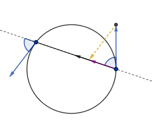
By lemma 2.9, it is sufficient to show that for data sampled from the unit circle in , the Bézier average with the mid-point of the circular arc determined by the data, and its ntangent.
Assume are sampled from a unit circle. We further assume w.l.o.g that and denote where . Basic geometrical reasoning shows that , and that if lies on the upper semicircle, namely if , then , while otherwise, . Using known trigonometric identities we obtain,
| (B.1) |
which is the parameter used in [8]. Therefore, by Theorem 1 in [8], the point of the Bézier average with weight of and is the midpoint of the circular arc defined by the two points and their ntangents.
To verify that the average tangent is tangent to the unit circle at , note that the tangent to the unit circle at is in the direction of . Observe as well that linearly depends on . In fact, it implies that:
| (B.2) |
and that . See Figure 9 for a graphical demonstration.


Proof of Lemma 3.1.
We prove that and satisfy conditions (2.8), namely,
- (i)
.
- (ii)
Let and . Then or are not pair-wise linearly dependent for .
First we prove (i). By algebraic manipulations we obtain that is equal to
|
|
Then, we argue that
| (B.4) |
and hence . In other words, .
To show that (B.4) holds, we observe that
Let
Then, , and . We define,
and obtain
To derive the critical points of , we observe that iff and similarly iff . In other words,
However, the only solution of the latter system of equations over is . Thus, we conclude that the minimum value of is obtained on the boundary of or in , which is also on the boundary (see Result A.1). We further explore all candidates of extremal points on the boundary of .
We consider the restriction of to the boundaries, which are functions of one variable, and get that
Now, iff ,namely at the point , while iff , namely at the point . Thus the above two equalities to are not satisfied simultaneously. Finally, by the continuity of and since for small enough and , we get that for any and conclude that . By symmetric reasoning we can show that also .
For the second claim, assume are pair-wise linearly dependent. That is, and for some . For simplicity we assume . We follow De Casteljau’s algorithm for obtaining and . As in (2.9), consider the initial control points of the associated Bézier curve and denote:
The following points are obtained by De Casteljau’s algorithm:
Then, and . For further information about De Casteljau’s algorithm, we refer the reader to [30]. Since , the points and lie on the same line. We denote this line by . Since , we have that and also lie on . is the average of and hence it also lies on . Now, since and lie on the same line, it follows that is on . Similarly, is on . Now is on since it lies on the line passing through and and finally we get that is on . Thus are pair-wise linearly dependent and hence, by our assumption, . It is shown in Lemma 2.10 that in this case as required. ∎
Proof of Lemma 3.3.
For the first part,
Since we have that and . In the same way we obtain . For the second claim of the lemma, simply set for any satisfying . ∎
Appendix C The set of the Bézier Average
The set consists of all pairs where the Bézier average is a Hermite average by Definition 2.2. Namely, for any pair in , the Bézier average fulfills the conditions (2.8) and produces averaged vectors in for any weight in . This section further investigates the properties of elements in to receive some perception of the size and significance of .
Let be a pair that meets the conditions (2.8). Then, following the notation of Section 2, iff of (2.11) is regular over . Nevertheless, recall that the regularity of depends on the parameters and of . In particular, to obtain regularity, the linearly independence of is sufficient; therefore, if do not lie on the same plane, then we conclude that . Thus, it remains to characterize the case where are in a two dimensional space.
Consider the vectors of difference between each two consecutive control points,
By Theorem 2 in [21], if the angles between each pair of those vectors are acute, then is regular. That is, if
| (C.1) |
Then, . The inner products in (C.1) are
| (C.2) |
Namely, if and for any , then .
In the plane we have the following relationship between and :
| (C.3) |
In Figure 10 we plot the domains of positivity of (C.2) for and for . Note that the first case is equivalent in sense of the positivity of (C.2) to the case where and therefore the latter is omitted. We consider the intersection of the domains in question, for both , together with . We conclude that even in the case where the control points lie on a plane (a rare event in high dimensions) the domain where is not minor.


The conditions on defined by the intersections, as presented in Figure 10, are sufficient to determine that . Nevertheless, these conditions are no necessary. To complete the picture, we briefly show a necessary conditions for a pair to be in .
Recall that we consider only the case when the control points are planer. Therefore, we assume, w.l.o.g, that for some arbitrary . In this case, and . Assigning the above to (2.12) yields:
Therefore, iff
| (C.4) |
The equations in (C.4) are quadratic in but transcendental in , and their absulote value sum and so we conclude that iff the system (C.4) has a solution in .